| Issue |
A&A
Volume 684, April 2024
|
|
|---|---|---|
| Article Number | A15 | |
| Number of page(s) | 23 | |
| Section | Galactic structure, stellar clusters and populations | |
| DOI | https://doi.org/10.1051/0004-6361/202348462 | |
| Published online | 28 March 2024 | |
M giants with IGRINS
III. Abundance trends for 21 elements in the solar neighborhood from high-resolution near-infrared spectra⋆
1
Division of Astrophysics, Department of Physics, Lund University, Box 43, 221 00 Lund, Sweden
e-mail: This email address is being protected from spambots. You need JavaScript enabled to view it.
2
Kapteyn Astronomical Institute, University of Groningen, Landleven 12, 9747 AD Groningen, The Netherlands
3
Department of Astronomy and McDonald Observatory, The University of Texas, Austin, TX 78712, USA
4
Materials Science and Applied Mathematics, Malmö University, 205 06 Malmö, Sweden
5
Observatoire de la Côte d’Azur, CNRS UMR 7293, BP4229, Laboratoire Lagrange, 06304 Nice Cedex 4, France
Received:
1
November
2023
Accepted:
8
January
2024
Abstract
Context. To be able to investigate the chemical history of the entire Milky Way, it is imperative to also study its dust-obscured regions in detail, as this is where most of the mass lies. The Galactic Center is an example of such a region. Due to the intervening dust along the line of sight, near-infrared spectroscopic investigations are necessary to study this region of interest.
Aims. The aim of this work is to demonstrate that M giants observed at high spectral resolution in the H- and K-bands (1.5–2.4 μm) can yield useful abundance ratio trends versus metallicity for 21 elements. These elements can then also be studied for heavily dust-obscured regions of the Galaxy, such as the Galactic Center. The abundance ratio trends will be important for further investigation of the Galactic chemical evolution in these regions.
Methods. We observed near-infrared spectra of 50 M giants in the solar neighborhood at high signal-to-noise and at a high spectral resolution with the IGRINS spectrometer on the Gemini South telescope. The full H- and K-bands were recorded simultaneously at R = 45 000. Using a manual spectral synthesis method, we determined the fundamental stellar parameters for these stars and derived the stellar abundances for 21 atomic elements, namely, F, Mg, Si, S, Ca, Na, Al, K, Sc, Ti, V, Cr, Mn, Co, Ni, Cu, Zn, Y, Ce, Nd, and Yb. We systematically studied useful spectral lines of all these elements in the H- and K-bands.
Results. We demonstrate that elements can be analyzed from H- and K-band high-resolution spectra, and we show which spectral lines can be used for an abundance analysis, identifying them line by line. We discuss the 21 abundance ratio trends and compare them with those determined from APOGEE and from the optical Giants in the Local Disk (GILD) sample. From high-resolution H- and K-band spectra, the trends of the heavy elements Cu, Zn, Y, Ce, Nd, and Yb can be retrieved. This opens up the nucleosynthetic channels, including the s-process and the r-process in dust-obscured populations. The [Mn/Fe] versus [Fe/H] trend is shown to be more or less flat at low metallicities, implying that existing non-local thermodynamic equilibrium correction is relevant.
Conclusions. With high-resolution near-infrared spectra, it is possible to determine reliable abundance ratio trends versus metallicity for 21 elements, including elements formed in several different nucleosynthetic channels. It is also possible to determine the important neutron-capture elements, both s- and r-dominated elements. This opens up the possibility to study the chemical evolution in detail of dust-obscured regions of the Milky Way, such as the Galactic Center. The M giants are useful bright probes for these regions and for future studies of extra-galactic stellar populations. A careful analysis of high-quality spectra is needed to retrieve all of these elements, which are often from weak and blended lines. A spectral resolution of R ≳ 40 000 is a further quality that helps in deriving precise abundances for this range of elements. In comparison to APOGEE, we can readily obtain the abundances for Cu, Ce, Nd, and Yb from the H-band, demonstrating an advantage of analyzing high-resolution spectra.
Key words: techniques: spectroscopic / stars: abundances / stars: late-type / Galaxy: abundances / solar neighborhood
The tables with line-by-line and mean abundances of all elements for the 50 stars are available at the CDS via anonymous ftp to cdsarc.cds.unistra.fr (130.79.128.5) or via https://cdsarc.cds.unistra.fr/viz-bin/cat/J/A+A/684/A15
© The Authors 2024
 Open Access article, published by EDP Sciences, under the terms of the Creative Commons Attribution License (https://creativecommons.org/licenses/by/4.0), which permits unrestricted use, distribution, and reproduction in any medium, provided the original work is properly cited.
This article is published in open access under the Subscribe to Open model. This email address is being protected from spambots. You need JavaScript enabled to view it. to support open access publication.
1. Introduction
In order to get a full picture of the formation and evolution of the Milky Way, the chemistry of its dust-obscured parts along the Galactic plane, where most of the mass lies, needs to be thoroughly investigated. However, dust prevents optical studies toward the inner Galactic plane, especially the Milky Way center. The possibility to investigate the chemistry through near-infrared observations is now maturing, opening up these areas for study (e.g., Frogel et al. 1999; Carr et al. 2000; Ramírez et al. 2000; Cunha et al. 2007; Rich et al. 2007, 2012; Ryde & Schultheis 2015; Ryde et al. 2016a, 2016b; Nandakumar et al. 2018; Guerço et al. 2022; Nieuwmunster et al. 2023). The main developments are toward more sensitive instruments and the possibility to efficiently record larger parts of the near-infrared spectrum, such as one or more full telluric transmission bands1 at once.
The stellar probes used for the chemical investigation of the inner regions of the Milky Way need to be bright. When K giants are not bright enough (e.g., in the Milky Way nuclear star cluster), methods to analyze the ubiquitous, brighter but cooler M giants in the near-infrared are needed. While the optical spectra of M giants are riddled with molecules, their near-infrared spectra (0.95–2.4 μm) can be analyzed (see, for example, the analysis in Hayes et al. 2022). We therefore need methods to retrieve stellar parameters and accurate and precise abundances from near-infrared spectra of not only K giants but also M giants.
Abundance determinations of local-disk stars have been performed based on optical high-resolution spectra for over 50 years, providing a large set of methods and spectral lines with accurate data from which one can obtain global stellar parameters and chemical abundances of stars. However, the near-infrared has been less explored than the optical, resulting in many unidentified spectral lines and often less accurate atomic data for those identified spectral lines of interest. As such, to determine adequate stellar parameters and chemical abundances, identifying usable lines and developing a careful analysis of high-resolution spectra is required. In this series of papers, we are trying to do just that.
In order to determine a range of nucleosynthetic channels and therefore a range of different elements, high spectral resolution (R ≳ 40 000) is needed. Several instruments with such capabilities, to a certain extent, exist already, such as the GIANO (Origlia et al. 2014), WINERED (Ikeda et al. 2007), and CRIRES+ (Follert et al. 2014) spectrographs and the IGRINS spectrometer (IGRINS; Yuk et al. 2010). In this study, we use IGRINS, which allows for observing spectra that covers both the H- and K-bands at high-resolution at once. IGRINS has been extensively used in a broad range of near-infrared spectroscopic studies, such as in the investigation of environments surrounding young stars (Kaplan et al. 2017, 2021), young stellar objects (Lee et al. 2016; Garro et al. 2023; López-Valdivia et al. 2023), planetary nebulae (Sterling et al. 2016; Madonna et al. 2018), very metal-poor stars (Afşar et al. 2016), carbon stars (García-Hernández et al. 2023), and evolved field stars, as well as those in open and globular clusters (e.g., Afşar et al. 2018; Böcek Topcu et al. 2019, 2020; Montelius et al. 2022; Afşar et al. 2023; Brady et al. 2023; Holanda et al. 2024). The urgent need to develop methods for deriving reliable stellar parameters and stellar abundances from high-resolution near-infrared spectra of M giants is relevant because the immense possibilities of observing more distant M giants will be expanded with upcoming instruments (such as ESO’s Multi-Object Optical and Near-infrared Spectrograph, MOONS, Cirasuolo et al. 2012) and future extremely large telescopes, such as ESO’s Extremely Large Telescope (ELT, Gilmozzi et al. 2008; Tamai & Spyromilio 2014) and the Thirty Meter Telescope (TMT, Skidmore et al. 2022), and the high-resolution near-infrared spectrometers projected for them (Maiolino et al. 2013; Genoni et al. 2016; Mawet et al. 2019).
Previous publications in this series are Nandakumar et al. (2023a, hereafter Paper I), and Nandakumar et al. (2023b, from hereon Paper II). In these works, we demonstrated a method for obtaining stellar parameters, α, and fluorine abundances for a set of 50 cool M giant stars in the solar neighborhood. In this paper, we extend the set of chemical abundances that are derived to include odd-Z, iron-peak, and neutron-capture elements, showing 21 elements in total apart from iron. This range of elements is important and opens the opportunity of obtaining the full chemical view of the Galaxy and its components. The neutron-capture elements especially introduce new nucleosynthetic channels with their own evolutionary timescales (see, e.g., Manea et al. 2023). Based on the method demonstrated in this study, it will now readily be possible to also investigate the massive, dust-obscured parts along the Galactic plane. Future infrared surveys and studies of the Galactic Center performed at high spectral resolution (R > 40 000) would therefore be rewarding.
The details of the observations and data reduction are provided in Sect. 2 and followed by an analysis in Sect. 3. In Sect. 4, we show the elemental abundance trends of the α, odd-z, iron-peak, and neutron-capture elements for the 50 solar neighborhood stars analyzed in this series. Further comparison with the trends from a well-studied optical giant star sample and from APOGEE are made in Sect. 5.
2. Observations and data reduction
We determined the abundances of 21 elements for 50 M giants (Teff < 4000 K) from high-resolution spectra observed with the Immersion GRating INfrared Spectrograph (IGRINS; Yuk et al. 2010; Wang et al. 2010; Gully-Santiago et al. 2012; Moon et al. 2012; Park et al. 2014; Jeong et al. 2014). These cool giants were selected from the APOGEE data release DR16 (Jönsson et al. 2020).
We observed the entire H- and K-bands (1.5–1.75 and 2.05–2.3 μm, respectively) at a spectral resolution of R ∼ 45 000, thus giving us access to a wealth of spectral lines and enabling a detailed study of a range of elements. Earlier abundance studies have shown the strength of high-resolution spectra recorded with IGRINS (see Afşar et al. 2018, 2023; Böcek Topcu et al. 2019, 2020; Montelius et al. 2022). For instance, Afşar et al. (2018) determined abundances for 21 elements for three horizontal-branch stars of 5000 < Teff < 5300 K showing a range of suitable spectral lines that are internally self-consistent. Some elements are better measured in the wavelength range of IGRINS than in the optical range.
All of the observed stars presented here lie in the solar neighborhood and serve as a good reference sample. A subset with 44 of these stars were observed with IGRINS mounted on the Gemini South telescope (Mace et al. 2018) within the programs GS-2020B-Q-305 and GS-2021A-Q302 from January to April 2021. The other six nearby M giants were available in the IGRINS spectral library (Park et al. 2018; Sawczynec et al. 2022) and were observed at the McDonald Observatory (Mace et al. 2016). Details of all these observations are provided in Paper I, where the stellar parameters and the [α/Fe] (Mg, Si, and Ca) and Ti are presented.
The spectral reductions were performed with the IGRINS PipeLine Package (IGRINS PLP; Lee et al. 2017) in order to optimally extract the telluric corrected, wavelength calibrated spectra after flat-field correction (Han et al. 2012; Oh et al. 2014). The spectra were then resampled and normalized in iraf (Tody et al. 1993), but to take care of any residual modulations in the continuum levels, we put considerable focus on defining specific local continua around every line that elemental abundances were determined from. Finally, the spectra were shifted to laboratory wavelengths in air after a stellar radial velocity correction. The average S/N2 of the spectra generally have S/N > 100.
3. Analysis
The spectroscopic analysis in this work was carried out using the spectral synthesis method wherein the stellar parameters and elemental abundances of a star are determined by fitting its observed spectrum with a synthetic spectrum. The synthetic spectrum was generated using the Spectroscopy Made Easy (SME; Valenti & Piskunov 1996, 2012) tool by calculating the spherical radiative transfer through a relevant stellar atmosphere model defined by its fundamental stellar parameters. We chose the stellar atmosphere model by interpolating in a grid of one-dimensional Model Atmospheres in a Radiative and Convective Scheme (MARCS) stellar atmosphere models (Gustafsson et al. 2008).
3.1. Stellar parameters
Fundamental stellar parameters, namely, the effective temperature (Teff), surface gravity (log g), metallicity ([Fe/H]), and microturbulence (ξmicro), are crucial in spectroscopic analyses. These parameters form the basis for a reliable determination of elemental abundances from respective absorption lines in the observed spectrum. Thus, it is important to determine accurate fundamental stellar parameters. Paper I devised a novel method to determine these parameters for M giants (Teff < 4000 K) through a spectral synthesis method that also employs SME and MARCS stellar atmosphere models. In this study, we use the same stars as in Paper I and the determined stellar parameters from that paper. In the method, a set of Teff-sensitive OH lines and a few chosen CO, CN and Fe lines are synthesized and fitted while setting Teff, [Fe/H], ξmicro, and the C and N abundance values as free parameters. The best-fit synthetic spectrum provided the values for these free parameters. The surface gravity, log g, is constrained based on the Teff and [Fe/H] values from 3–10 Gyr Yonsei-Yale isochrones (Demarque et al. 2004). The main assumption in this method is the value of oxygen abundance that is taken from a simple functional form of the [O/Fe] versus [Fe/H] trend in Amarsi et al. (2019) for thin- and thick-disk stars (see also Fig. 1 in Paper I).
The method was validated in Paper I by determining the stellar parameters for the stars also analyzed here. The six nearby, well-studied M giants with well-determined stellar parameters were used to benchmark the method. Furthermore, reliable α-element trends versus metallicity were determined for the stars in Paper I in order to showcase the accuracy and precision of the derived stellar parameters. These stellar parameters are given in Table 2 in Paper II. The derived stellar parameters are in the range of 3350 to 3800 K in Teff, 0.3 to 1.15 dex in log g, and −0.9 to 0.25 dex in [Fe/H]. The separation into the high-α and low-α populations was originally based on the magnesium abundances determined by APOGEE. Our magnesium abundance estimates in Paper I (also see Sect. 4.2 and Fig. 2 in this work) further confirms this classification.
3.2. Line list
For the spectral synthesis, we used a line list containing the wavelengths of the spectral lines, line strengths in the form of log gf-values, excitation energies, broadening parameters, and hyperfine splitting values, if necessary. As a starting point, we used an updated version of the VALD line list (Piskunov et al. 1995; Kupka et al. 2000; Ryabchikova et al. 2015). For the many lines that lack reliable experimental transition probabilities, we estimated log gf-values by determining them astrophysically. The log gf-values for the H-band lines were determined from a high S/N reflected solar spectrum of Ceres measured with IGRINS (Montelius 2021). The values were validated by computing abundances of some 34 K giants and comparing them to high-resolution optical abundances from the Giants in the Local Disk sample (GILD; Jönsson et al., in prep.). For the K-band lines, we determined log gf-values using the high-resolution infrared solar flux spectrum of Wallace & Livingston (2003) and testing them on the high-resolution (R ∼ 100 000) infrared spectrum of the bright giant Arcturus3 from the Arcturus atlas (Hinkle et al. 1995). For lines with hyperfine structure splitting, the log gf-values were assigned according to their relative line strength within the LS multiplet (Cowan 1981; Montelius 2021).
For many lines, we adopted the broadening parameters from the ABO theory (Anstee & O’Mara 1991; Anstee & O’Mara 1995; Barklem & O’Mara 1997; Barklem et al. 1998) or from the spectral synthesis code BSYN based on routines from MARCS (Gustafsson et al. 2008). The line data for the CO, CN, and OH lines were adopted from the line lists of Li et al. (2015), Brooke et al. (2016), and Sneden et al. (2014), respectively. The molecular lines are important since they often act as blending lines in atomic spectral lines.
The details of the lines for the elements Mg, Si, Ca (except for the six new lines in this work), Ti, F, and Yb are provided in Paper I, Paper II, and Montelius et al. (2022). The details about the H-band lines used in this work, except for cerium and neodymium, can be found in Montelius (2021). We provide the details about cerium and neodymium H-band lines and K-band lines of other elements below4.
Sulfur. For the K-band sulfur line (S I), we adjusted the log gf-value from theoretical calculations in Biemont et al. (1993) to fit the line in the high-resolution solar spectrum. The broadening value for the line is adopted from the ABO theory.
Sodium. For the three K-band sodium lines (NaI), hyperfine transition information and log gf-values are available in the VALD line list. These values were originally determined experimentally from Arqueros (1988). Broadening parameters were determined from the ABO theory for all three lines. The wavelengths of the first two lines had to be shifted forward by ∼0.1 Å in order to fit them in the high-resolution spectra of the Sun and Arcturus with synthetic spectra.
Aluminum. Among the three K-band aluminum lines (AlI), VALD provides hyperfine transition lines from Chang (1990) for the first two lines and no line information for the third line. Nordlander & Lind (2017) provides line data for all three lines but only one wavelength per line for the first two lines (i.e., no hyperfine transition information). We could also fit these lines in the high-resolution spectra of the Sun and Arcturus with the line data from Nordlander & Lind (2017). The abundances determined for the stars in this work from the first two lines with line data from VALD were found to be lower by ∼0.2 dex compared to those determined with line data from Nordlander & Lind (2017). Hence, we adopted the line data from Nordlander & Lind (2017) for all three K-band aluminum lines in order to determine abundances.
Calcium. We have included six K-band calcium (CaI) lines in addition to the five lines in the H- and K-bands used in Paper I. We updated the log gf-values of all six lines astrophysically using the high-resolution solar spectrum, and we tested them using high-resolution Arcturus spectrum.
Scandium. The line list extracted from VALD provided the hyperfine structure information for the three scandium lines (ScII) in the K-band from Ertmer & Hofer (1976) and Aboussaïd et al. (1996). We adopted the log gf-values from Pehlivan et al. (2015), who determined them based on laboratory measurements. In addition, we shifted the wavelengths of the second and third line by 0.13 Å and 0.05 Å respectively to fit them in the high-resolution spectra of the Sun and Arcturus.
Nickel. In addition to the H-band lines, five K-band nickel lines (NiI) were used to determine nickel abundances in this work. The log gf-values for these lines from the VALD database are from Kurucz (2008). Only two lines in the high-resolution spectra of the Sun and Arcturus were fit by synthetic spectra using the VALD log gf-values. We estimated astrophysical log gf-values for the remaining three lines.
Yttrium. The two ionized yttrium lines (Y II) in the K-band used in this work are weak in the high-resolution spectra of the Sun and Arcturus and thus made it difficult to reliably estimate astrophysical log gf-values. In addition, there is no information on the hyperfine transitions for these lines. Hence, we adopted the line data provided by VALD from Kurucz (2006). The only way we could determine the reliability of these lines and their log gf-values was by inspecting the synthetic spectra fit to the observed lines that are stronger in cool M giants and then comparing the resulting abundance trends with the trends derived from well-studied lines in optical spectra (see the discussion in Sects. 4.6.2 and 5).
Cerium. Cunha et al. (2017) determined astrophysical log gf-values for ionized cerium lines (CeII) in the H-band using a combination of a high-resolution Fourier Transform Spectrometer (FTS) spectrum of Arcturus and an APOGEE spectrum of a metal-poor but s-process-enriched red giant star. We adopted these log gf-values for the four cerium lines used in this work to determine cerium abundances.
Neodymium. We used the log gf-values of the three ionized neodymium lines (NdII) in the H-band determined astrophysically in Hasselquist et al. (2016). The metal-poor, K giant 2MASSJ16011638-1201525 was used in Hasselquist et al. (2016) to determine the log gf-values for these lines.
3.3. Non-local thermodynamic equilibrium grids
We included non-local thermodynamic equilibrium (NLTE) grids for the elements C, N, O, Na, Mg, Al, Si, K, Ca, Mn, and Fe (Amarsi et al. 2020, Lind et al. 2017 and Amarsi et al. 2016 with subsequent updates; Amarsi priv. comm.). The departure coefficients were computed using the MPI-parallelized NLTE radiative transfer code Balder (Amarsi et al. 2018).
4. Results
We determined the metallicities and chemical abundances of 21 elements for the sample of 50 M giants in the solar neighborhood. In this section, we show the abundance trends for these elements determined from each elemental line as well as the mean estimated abundances as a function of metallicity after the careful removal of abundances determined from bad, noisy lines and those affected by strong telluric contamination. We grouped them as α-, odd-Z, iron-peak, and neutron-capture elements. We discuss fluorine separately. The tables with line-by-line and mean abundances of all elements for the 50 stars will be made available online.
We chose the metal-rich star 2M14261117–6240220 to determine uncertainties in estimated abundances for all 21 elements resulting from the typical uncertainties in the stellar parameters. We followed the method described in Paper I, where we redetermined 50 values of the abundances from all selected lines of each element by setting the stellar parameters to randomly chosen values from normal distributions, with the actual stellar parameter value as the mean and the typical uncertainties (±100 K in Teff, ±0.2 dex in log g, ±0.1 dex in [Fe/H], and ±0.1 km s−1 in ξmicro) as the standard deviation. The uncertainty in the abundance determined from each line was then taken to be the mid-value of the difference between the 84th and 16th percentiles of the abundance distribution. The final abundance uncertainty was the standard error of the mean of uncertainties from all chosen lines of each element. The mean uncertainties range from 0.04 to 0.12 dex, with the maximum uncertainty of 0.12 dex estimated for sulfur.
For all elements except fluorine and cerium, we scaled the abundances with respect to solar abundance values from Grevesse et al. (2007). We used A⊙(F) = 4.43 from Lodders (2003) and A⊙(Ce) = 1.58 from Grevesse et al. (2015) for fluorine and cerium, respectively.
4.1. Fluorine (F)
The fluorine abundances were determined from HF molecular lines in the K-band. Paper II carried out a detailed analysis of ten vibrational-rotational, R-branch lines in IGRINS spectra of the 50 solar neighborhood stars used in this work. This was done to find the best set of HF lines from which to determine the fluorine abundances for this type of star while avoiding saturated lines. Paper II suggested to use the three bluest HF lines for cool (Teff < 3500 K) and metal-rich ([Fe/H] > 0 dex) M giants and three additional lines for M giants at sub-solar metallicities. All HF lines are intrinsically very temperature sensitive, which means that we should expect a larger spread in the derived fluorine abundances. We found a flat [F/Fe] versus [Fe/H] trend but with indications of a slightly higher level of [F/Fe] for stars with [Fe/H] > 0 dex in the solar neighborhood sample (see Fig. 1; also presented in Paper II).
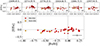 |
Fig. 1. [F/Fe] versus [Fe/H] trends for 50 M giants in our sample. Figures in the upper panel show the trends determined from five individual HF lines. The mean [F/Fe] versus [Fe/H] trend from all six lines is shown in the bottom panel. Red filled circles and orange diamonds denote the thin- and thick-disk stars, respectively. The error bar in the bottom-right part of the top panels and the bottom panel indicate the uncertainties in abundances determined from each line and the mean uncertainty determined as the standard error of mean (see text in the Sect. 4 for more details). |
4.2. α-elements (Mg, Si, S, and Ca)
Magnesium, silicon, sulfur, and calcium. The α-elements are the most commonly studied group of elements and have very well-investigated abundance trends for different Milky Way stellar populations. We determined the abundances of magnesium (Mg), silicon (Si), sulfur (S), and calcium (Ca) from multiple lines in the H- and K-bands (see Fig. A.2). For Mg and Si, we determined abundances from the same lines as used in Paper I. We also used NLTE corrections for Mg, Si, and Ca lines.
For sulfur, we used one H-band line and one K-band line to determine its abundances. For calcium, we used six more lines than used in Paper I in the K-band, resulting in a total of 11 Ca lines. The abundance trends for Mg, Si, S, and Ca are shown in Figs. 2–5, respectively, with the trends from each individual line in the top panels and the mean abundance estimated from all lines in the bottom panel. The solar neighborhood thin- and thick-disk stars in each figure are shown by red filled circles and orange diamonds, respectively. Except in the case of Mg, for which only K-band lines were used, both H- and K-band lines have been used to determine the abundances for rest of the α-elements.
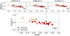 |
Fig. 2. [Mg/Fe] versus [Fe/H] for 50 M giants in our sample. The arrangement of the figures and markers is similar to Fig. 1. |
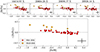 |
Fig. 3. [Si/Fe] versus [Fe/H] for 50 M giants in our sample. The arrangement of the figures and markers is similar to Fig. 1. |
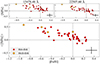 |
Fig. 4. [S/Fe] versus [Fe/H] for 48 M giants in our sample. The arrangement of the figures and markers is similar to Fig. 1. |
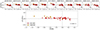 |
Fig. 5. [Ca/Fe] versus [Fe/H] for 50 M giants in our sample. The arrangement of the figures and markers is similar to Fig. 1. |
There is a clear enhancement in the mean abundances of all α-elements (though it is not as clear for the sulfur abundances) for the solar neighborhood thick-disk stars, leading to a separation between the thin- and thick-disk populations. This has also been seen in the optical analyses for Mg, Si, and Ca (see, for instance, Jönsson et al. 2017), but less so for S (see, e.g., Costa Silva et al. 2020; Perdigon et al. 2021). This separation is more evident in the metal-poor regime ([Fe/H] < –0.4 dex), where five out of the six thick-disk stars lie. Except for Si, there is no clear enhancement seen for the thick-disk star with solar metallicity. As mentioned in Paper I, this is possibly due the fact that the Si abundance was only determined from one good line, 16 434.93 Å.
We chose to list Ti among the iron-peak elements (see also Sneden et al. 2016) and not as an α-element since the nucleosynthetic formation channel of the main isotope 48Ti is through the decay of the radioactive 48Cr isotope in Si-burning zones in core-collapse supernovae (Curtis et al. 2019). Therefore, Ti can primarily be considered as an iron-peak element. Chromium is created in SNe Ia and SNe II in comparable amounts (Clayton 2003; Lomaeva et al. 2019).
4.3. Odd-Z elements (Na, Al, and K)
Among the odd-Z elements, we determined abundances of sodium (Na), aluminum (Al), and potassium (K). For the determination of the Na and Al abundances, we used lines from both the H- and K-bands, while only two H-band lines were used to determine K abundances (see Fig. A.3).
Sodium. The sodium abundances from each line show an increasing [Na/Fe] trend with an increase in metallicity (see Fig. 6). For sodium, we used NLTE corrections. At sub-solar metallicities, the Na abundances determined from the two H-band lines have super-solar values, whereas the lines in the K-band have sub-solar values resulting in larger positive slopes. The trend found for local dwarfs by Bensby et al. (2014) and for local giants by GILD (see Fig. 27), both without NLTE corrections, are consistent with the trend determined using the two H-band lines.
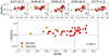 |
Fig. 6. [Na/Fe] versus [Fe/H] for 50 M giants in our sample. The arrangement of the figures and markers is similar to Fig. 1. We exclude [Na/Fe] abundances from the three K-band lines to estimate the mean [Na/Fe] abundance since the abundances from these lines are sub-solar for the sub-solar metallicity stars. This is inconsistent with the abundances from H-band lines, as well as in APOGEE and other optical studies (see also Figs. 25–27). |
The difference between the trends of the H- and K-band line abundances can be attributed to the NLTE corrections to the three K-band line abundances from Amarsi et al. (2020). Figure 7 shows the NLTE-LTE differences in the [Na/Fe] abundances determined from each line for all stars. The NLTE corrections to the H-band line abundances are very low (≲ − 0.1 dex) for all [Fe/H]. Meanwhile, there is a large variation in the NLTE corrections to the K-band lines that range from ∼ − 0.4 dex to ∼ − 0.1 dex. Hence, one plausible explanation for the sub-solar [Na/Fe] values determined from the K-band lines at sub-solar metallicities is that the NLTE corrections are too large for these metallicities. Abundances determined from the different lines should ideally yield the same abundance trends. In their work involving the characterization of two low-latitude star cluster candidates toward the Galactic bulge with IGRINS, Lim et al. (2022) found significant and systematic discrepancies between some abundance ratios measured from H- and K-band spectra, particularly for Al, Ca, and Ti. They identified NLTE effects as one of the possible reasons (in addition to the effects of atmosphere parameters and atomic parameters) for this and also found that abundance differences are reduced by NLTE corrections but not eliminated completely.
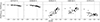 |
Fig. 7. NLTE-LTE differences versus [Fe/H] for sodium (Na) abundances from the two H-band and three K-band lines for 50 M giants in our sample. NLTE corrections are higher and ranges from ∼ − 0.4 dex to ∼ − 0.1 dex for the K-band lines. |
Thus, we excluded Na abundances from the three K-band lines while determining the mean [Na/Fe] abundances in the bottom panel of Fig. 6. The final, mean [Na/Fe] trend resembles the trend found for local dwarfs by Bensby et al. (2014) with a stretched-out N-shape. The trend for the metal-poor thick-disk stars shows a hint of a separate trend compared to that of the thin-disk stars, following the upper envelope of the thin-disk trend. Furthermore, the thick-disk trend seems to turn down for decreasing metallicities, which is also expected from chemical evolution models (see, for example, Kobayashi et al. 2020).
Aluminum. We determined Al abundances from seven lines, four of them in the H-band and three in the K-band and all with NLTE corrections. There are differences in the abundance trends from each line in terms of the determined values and the magnitude of scatter (see Fig. 8). The mean [Al/Fe] values (bottom panel of the figure) determined from all the lines show a clear difference between the thin- and thick-disk stars. The mean [Al/Fe] of the solar neighborhood thin-disk stars is generally near solar (in the super-solar regime), which is a bit lower compared to the clearly increasing slope for decreasing metallicities found in local dwarfs (Bensby et al. 2014). But we observed a clear slope in the trends from individual Al lines. The solar neighborhood thick-disk stars are enhanced by ∼0.2 dex, and the aluminum abundance trend decreases as metallicity decreases, which is also expected from chemical evolution models (see, for example, Kobayashi et al. 2020).
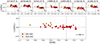 |
Fig. 8. [Al/Fe] versus [Fe/H] for 50 M giants in our sample. The arrangement of the figures and markers is similar to Fig. 1. |
Potassium. To determine the [K/Fe] abundances, two neighboring H-band lines separated by ∼5 Å were used (see Fig. 9). We used NLTE corrections for potassium. For the metal-poor thick-disk stars, there is a clear enhancement in [K/Fe], as determined from both lines. It was not found in the study by Takeda (2019) but is in APOGEE for K giants (see, e.g., Fridén 2023). The mean [K/Fe] values for the thin-disk stars are slightly sub-solar and show a slightly declining trend, as expected form optical observations and models (Takeda et al. 2002; Prantzos et al. 2018; Takeda 2019). We note that there are not many studies on the Galactic evolution of K in Milky Way disks.
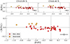 |
Fig. 9. [K/Fe] versus [Fe/H] for 48 M giants in our sample. The arrangement of the figures and markers is similar to Fig. 1. |
4.4. Iron-peak elements (Sc, Ti, V, Cr, Mn, Co, and Ni)
We determined the abundances of all seven iron-peak elements: scandium (Sc), titanium (Ti), vanadium (V), chromium (Cr), manganese (Mn), cobalt (Co), and nickel (Ni). Both H- and K-band lines were used to determine the titanium and nickel abundances. Only K-band lines were used to determine the abundance of Sc, and only H-band lines were used to determine abundances for the other iron-peak elements (see Fig. A.4).
Scandium. All three Sc lines showed a similar trend (see Fig. 10). The mean [Sc/Fe] trend showed a hint of a generally decreasing slope with metallicity, with the thick-disk stars showing higher Sc abundances than those of the thin-disk. This is similar to the trend for disk dwarfs and giants in Battistini & Bensby (2015) and Lomaeva et al. (2019), respectively. We note that the scatter in our data for super-solar metallicities are larger than in the optical studies. One plausible explanation for this scatter is that the K-band ScI lines have been found to be very Teff-sensitive, especially at Teff < 4000 K, (see, e.g., Thorsbro et al. 2018), which means that we should expect a larger scatter, just like for fluorine.
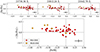 |
Fig. 10. [Sc/Fe] versus [Fe/H] for 50 M giants in our sample. The arrangement of the figures and markers is similar to Fig. 1. |
Titanium. For Ti, we determined abundances from the same two lines used in Paper I, one in the H-band and one in the K-band, with the former showing the tightest trend (see Fig. 11). The thick-disk is clearly separated from the thin-disk, resembling the dwarf-star trends in Bensby et al. (2014) or the giant-star trends in Jönsson et al. (2017), Lomaeva et al. (2019).
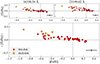 |
Fig. 11. [Ti/Fe] versus [Fe/H] for 50 M giants in our sample. The arrangement of the figures and markers is similar to Fig. 1. |
Vanadium. We determined the [V/Fe] abundances from one H-band line. Thin-disk stars were found to have sub-solar values, and metal-poor thick-disk stars were found to have enhanced super-solar values (see Fig. 12). Based on optical analyses, both the dwarf-star trend in Battistini & Bensby (2015) and the giant-star trend in Lomaeva et al. (2019) show similar enhancement for the thick-disk stars in their sample, although their trends are higher by 0.1–0.2 dex.
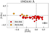 |
Fig. 12. [V/Fe] versus [Fe/H] for 50 M giants in our sample. The arrangement of the figures and markers is similar to Fig. 1. |
Chromium. The [Cr/Fe] trend is flat. The Cr abundances determined from the two lines at bluer wavelengths in the H-band are sub-solar for both thin- and thick-disk stars and showed a tight trend (see Fig. 13). The [Cr/Fe] abundances determined from the reddest wavelength line is more uncertain since this wavelength region has some significant telluric lines affecting the quality of the spectra. The trend derived from this line is largely solar for metal-poor stars and super-solar at high metallicities, with an increased scatter (see Fig. 13). The mean [Cr/Fe] values are, however, mainly sub-solar at all metallicities, with the slightly larger scatter for metal-rich stars mainly caused by this reddest line. Overall, our chromium abundances exhibit the expected flat trend versus metallicity. The abundance differences between the thin- and thick-disk stars is small, although the metal-poor thick-disk stars showed a consistent enhancement in [Cr/Fe] compared to the thin-disk stars from all three lines. This is very similar to the finding from the optical analysis for giants in Lomaeva et al. (2019).
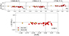 |
Fig. 13. [Cr/Fe] versus [Fe/H] for 50 M giants in our sample. The arrangement of the figures and markers is similar to Fig. 1. |
Manganese. Manganese is of special interest since its abundance trends depend on the properties and type of the Type-Ia-supernovae progenitors (de los Reyes et al. 2020), and there are indications of metallicity-dependent SNe II yields (Woosley & Weaver 1995). However, its chemical evolution trends are debated. A range of optical and near-infrared trends as well as Galactic chemical evolution models have shown an increasing trend with metallicity (Battistini & Bensby 2015; Zasowski et al. 2019; Lomaeva et al. 2019; Kobayashi & Nakasato 2011; Vasini et al. 2024). On the other hand, Bergemann & Gehren (2008) found that NLTE abundances are larger, especially for the most metal-poor stars, with correction up to 0.5 dex. This would lead to an essentially flat trend with metallicity (see also Battistini & Bensby 2015; Lomaeva et al. 2019), with the yields being less metallicity dependent. The question to investigate is whether the chemical evolution models or the NLTE corrections need modifications.
In the analysis of K giants (Teff > 4000 K) by Montelius (2021), Mn abundances were determined from high-resolution IGRINS spectra using the two Mn lines at 15 218 and 15 262 Å, including the important hyperfine structure components. He found a considerably flatter trend, especially at sub-solar metallicities, compared to what was found earlier. He included NLTE corrections based on the calculations by Amarsi et al. (2020), which are shown with the inverted dark-red triangles in the bottom panel of Fig. 15. They are positive for all the stars with Teff > 4000 K. In the earlier optical studies, the NLTE corrections are also positive, flattening the positive slope at low metallicities (Bergemann et al. 2019). Fridén (2023) confirmed the flat trend when comparing a set of stars analyzed both by APOGEE and IGRINS; he did not find the increasing Mn abundances for increasing metallicity as provided by APOGEE.
In this work, we analyzed cooler stars (Teff < 4000 K) observed with the same high spectral resolution IGRINS spectrometer and determined manganese abundances from the same two lines including the NLTE corrections from Amarsi et al. (2020). In Fig. 14, our mean [Mn/Fe] trend confirms the flat trend at [Fe/H] < –0.2, and here the NLTE corrections are negligible for the coolest stars (see filled circles in the bottom panel of Fig. 15), and the lines can, therefore, be assumed to have formed in LTE conditions. For higher metallicities, we observed a large scatter and an increasing trend. In the upper panel of Fig. 15, we plot the [Mn/Fe] abundances determined in this work and for the warmer stars (Teff > 4000 K) analyzed in Montelius (2021), which are color coded in Teff with circles and triangles, respectively, including the NLTE corrections. The trend is flat for nearly all stars when including these corrections, except for the coolest, metal-rich stars.
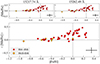 |
Fig. 14. [Mn/Fe] versus [Fe/H] for 50 M giants in our sample. The arrangement of the figures and markers is similar to Fig. 1. |
For the warmer stars of Montelius (2021) and for our warmer cool stars (Teff > 3550 − 4000 K), there is no temperature dependence of the derived abundances, and these stars showed a flat trend also at high metallicities. This is expected since the abundance should not depend on the temperature of the stars. However, for the coolest stars, there is a clear and unwanted Teff-dependence of the overabundance of Mn for super-solar metallicities. This shows that we cannot trust the Mn abundances for the coolest stars for super-solar metallicities. This could be caused by the temperature dependence of the NLTE corrections being too small. The NLTE corrections are negligible for the metal-poor stars, but for the more metal-rich stars, the corrections are larger and lead to a lowering of the derived abundances (see the lower panel in Fig. 15). This would mean that the NLTE correction would need to be larger in order to lower the [Mn/Fe] abundances down to the trend shown by the warmer stars. Another reason for the overabundance of Mn could be related to general difficulties in the analysis of the coolest stars. For these cool, metal-rich stars, the Mn lines become increasingly stronger with the risk of getting saturated, which means that the uncertain microturbulence will affect the abundance determination more than desired. The wavelength region is, however, quite free from telluric contamination.
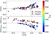 |
Fig. 15. Manganese abundance trends and NLTE-LTE differences as a function of [Fe/H] for 50 M giants in this work and 38 K giants in Montelius (2021). Upper panel: [Mn/Fe] versus [Fe/H] for solar neighborhood M giants in this work (filled circles) and for the warmer K giants (Teff > 4000 K) analyzed in Montelius (2021) (inverted triangles) color coded in Teff and including the NLTE corrections and determined from the same H-band lines. Bottom panel: NLTE corrections (NLTE-LTE) to manganese abundances based on the calculations by Amarsi et al. (2020) for M giants in this work and K giants analyzed in Montelius (2021). Markers are the same as in the upper panel. The NLTE corrections for the abundance derived from these lines depend on the effective temperatures of the stars. |
Thus, the abundance analyses of the Mn trends from high-resolution near-infrared stellar spectra of cool metal-poor stars based on lines that are formed, more or less, in LTE conditions indicate that the flat [Mn/Fe] versus [Fe/H] trend is presumably correct and that the nucleosynthesis of Mn is therefore empirically more like a normal iron-peak element. The flat trend is strengthened by other studies based on optical and near-infrared lines; however, these studies require NLTE corrections (see, e.g., Bensby et al. 2014). The fact that the metallicity-dependent NLTE corrections are different for different lines (optical and near-infrared) and very different for different Teff of the stars (see Fig. 15) indicates that the NLTE corrections are correct for optical and near-infrared spectral lines (but not for the coolest and most metal-rich stars) and that the cosmic nucleosynthesis of Mn is thus still uncertain.
Cobalt. Only one line was used to determine the [Co/Fe] abundances, from which we obtained a very tight trend with very low scatter (see Fig. 16). The trend for the thin-disk stars starts with super-solar values at the lowest metallicities, and they transition to sub-solar values at [Fe/H] ∼ –0.4 dex and continue at sub-solar values as the metallicity increases. All five metal-poor thick-disk stars have enhanced [Co/Fe] values, and the solar metallicity thick-disk star has a solar [Co/Fe] value that is closer to the thin-disk stars. The thin- and thick-disk trends are clearly separated. These trends follow the dwarf-star trends found in Battistini & Bensby (2015), although our trends are systematically lower by ∼0.1 dex. The trend is also very similar to the giant trend from the optical analysis by Lomaeva et al. (2019), although their trend is also higher by 0.1 − 0.2 dex.
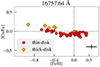 |
Fig. 16. [Co/Fe] versus [Fe/H] for 50 M giants in our sample. The arrangement of the figures and markers is similar to Fig. 1. |
Nickel. To determine the [Ni/Fe] abundances, we used six lines in the H-band and five lines in the K-band. There are significant differences in the measured abundances and dispersion or scatter from each line (see Fig. 17). The mean [Ni/Fe] values for the thin-disk stars, though, showed a tight trend that increases slightly with increasing metallicity. This is very similar to the dwarf-star trend in Bensby et al. (2014) and giant trend in Lomaeva et al. (2019). The thick-disk stars showed enhancements with super-solar values.
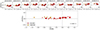 |
Fig. 17. [Ni/Fe] versus [Fe/H] for 50 M giants in our sample. The arrangement of the figures and markers is similar to Fig. 1. |
4.5. Transition elements between iron-peak and neutron-capture elements (Zn)
The elements after Ni transition to the weak s-dominated elements (nuclides with mass numbers up to A = 90; Prantzos et al. 2018). There are strong observational indications that Cu has a mainly weak s origin (e.g., Delgado Mena et al. 2017; Ernandes et al. 2020). The origin of Zn is, however, complex and uncertain. According to Clayton (2003), it is indeed synthesized by the weak s-process but also through radioactive decay from products synthesized in explosive nucleosynthesis in core-collapse supernovae through alpha-rich freeze out.
Zinc. We measured the zinc abundance from only one H-band line, which makes it less certain. The abundance trend resembles an α-element, as it decreases with metallicity (see Fig. 18). The thick-disk trend is marginally higher than that of the thin disk. It is obvious that the Zn trend is not similar to the trend of Cu, which is, as mentioned, mainly synthesized by the weak s-process (see Sect. 4.6.1). This is interesting since the weak s-process also contributes to the origin of Zn to a certain degree. Although similar to the trend of da Silveira et al. (2018), our trend shows a larger negative slope as the metallicity grows compared to other optical studies, such as Mishenina et al. (2002), Bensby et al. (2014), Delgado Mena et al. (2017). All these studies, however, show a flatter trend than the metallicity-dependent secondary behavior (weak s) trend that Cu shows. For example, Mishenina et al. (2002) clearly demonstrate in a [Cu/Zn] trend that the [Cu/Fe] trend is more metallicity dependent than that of [Zn/Fe]. This shows a clear empirical difference between the cosmic origin of Cu and Zn.
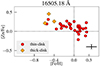 |
Fig. 18. [Zn/Fe] versus [Fe/H] for 35 M giants in our sample. The arrangement of the figures and markers is similar to Fig. 1. |
4.6. Neutron-capture elements (Cu, Y, Ce, Nd, and Yb)
We determined the abundances of copper (Cu), yttrium (Y), cerium (Ce), neodymium (Nd), and ytterbium (Yb), which are all mainly synthesized by neutron-capture processes. Copper is synthesized primarily in the weak s-process in massive stars as a secondary element (e.g., Pignatari et al. 2010; Ernandes et al. 2020; Baratella et al. 2021). However, to some extent, it is also synthesized in explosive nucleosynthesis in the inner shells of core-collapse supernovae through alpha-rich freeze out as a primary element (e.g., Pignatari et al. 2010).
Most neutron-capture elements are produced by a combination of the s- and r-processes. For Y and Ce, the main s-process dominates with s/r = 70/30 [in %] and 85/15, respectively, in the solar isotopic mixture (Bisterzo et al. 2014; Prantzos et al. 2020). Neodymium has an s/r = 60/40 ratio and can therefore still be considered as a predominantly s-process element. On the other hand, ytterbium has a ratio close to 50/50 (Bisterzo et al. 2014; Prantzos et al. 2020; Kobayashi et al. 2020), which makes it the element with the highest contribution from the r-process in its origin among the elements presented in this study. The more the r-process contributes, the more the abundance trends resemble and reveal an r-process contribution.
While only K-band lines were used in the case of yttrium, only H-band lines were used for the copper, cerium, neodymium, and ytterbium abundance determinations. Figure A.5 shows the H- and K-band lines of neutron-capture elements used in this study.
4.6.1. Weak s-elements (Cu)
Copper. Both of the lines used to determine the copper abundance are weak, and the long-wavelength wing of the bluest line is somewhat blended with an Fe I line-wing (see Fig. A.5). As a result, reliable Cu abundances could only be determined for a few stars (see Fig. 19). The mean [Cu/Fe] abundances show a wave-like trend starting off at slightly super-solar values at the lowest metallicities then decreasing to sub-solar values at sub-solar metallicities and then again increasing at super-solar metallicities. The thick-disk stars tend to lie above the thin-disk stars. These solar neighborhood trends follow the expected trends seen in optical studies of both dwarfs and giants (see, for e.g., Delgado Mena et al. 2017; Forsberg 2023).
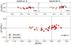 |
Fig. 19. [Cu/Fe] versus [Fe/H] for 36 M giants in our sample. The arrangement of the figures and markers is similar to Fig. 1. |
4.6.2. Elements dominated by the s-process (Y, Ce, and Nd)
Yttrium. The derived yttrium abundances from the two K-band lines show similar sub-solar values and show a similar scatter and trends as a function of metallicity (see Fig. 20). The thick-disk stars have [Y/Fe] values that follow the lower envelope of the thin-disk trend. The scatter, or the broad distribution of [Y/Fe] abundances for a given metallicity for the thin-disk stars, as well as the fact that the thick-disk trend lies below the thin-disk “cloud” is also seen in [Y/Fe] versus [Fe/H] trends from optical studies (a clear example can be seen in Tautvaišienė et al. 2021; Forsberg 2023). This is also expected from theoretical Galactic chemical evolution models of, for example, Zr, which has a behavior similar to Y (Grisoni et al. 2020). The scatter in the thin-disk distribution is most likely real and therefore of cosmic origin and not from measurement uncertainties.
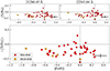 |
Fig. 20. [Y/Fe] versus [Fe/H] for 50 M giants in our sample. The arrangement of the figures and markers is similar to Fig. 1. |
The normalization in which the solar neighborhood trend for the thin-disk is expected to go through the solar abundance ratio at [Fe/H] = 0 is comparable to the optical determined trend (see Fig. 27 in Sect. 5.1.3). This indicates that the log gf-values obtained from VALD might not be too unreliable for these yttrium lines and can be utilized to obtain reliable abundances (see Sect. 3.2).
Cerium. The [Ce/Fe] versus [Fe/H] trends from all four lines are similar, with a downward trend, that is, the super-solar metallicity stars were found to have the lowest [Ce/Fe] values (see Fig. 21). Just as in the case of the trend for yttrium, the thick-disk stars follow the lower envelope of the thin-disk trend. The similar scatter, or broad distribution, in [Ce/Fe] abundances for a given metallicity has also been clearly seen in studies of optical lines for solar neighborhood giants (see e.g., Battistini & Bensby 2016; Delgado Mena et al. 2017; Forsberg et al. 2019; Tautvaišienė et al. 2021) and from near-infrared lines in the APOGEE Open Cluster Chemical Abundances and Mapping survey (Sales-Silva et al. 2022). The normalization in which the solar neighborhood trend for the thin-disk is expected to go through the solar abundance ratio at [Fe/H] = 0 is too low for our near-infrared determination as compared to the optical, and this indicates that the log gf-values might be too strong, leading to too-low derived abundances of Ce from these lines.
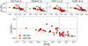 |
Fig. 21. [Ce/Fe] versus [Fe/H] for 50 M giants in our sample. The arrangement of the figures and markers is similar to Fig. 1. |
Neodymium. The [Nd/Fe] abundances were determined from three H-band lines that show similar trends (see Fig. 22). The [Nd/Fe] determinations for the thick-disk stars follow the lower envelope of the thin-disk. These trends fit well in the overall picture of neutron-capture elements in the disk components found in Tautvaišienė et al. (2021), Forsberg (2023), with the thick-disk following the lower envelope of the thin-disk “cloud”. These features are also found in the cases of the s-process dominated elements Y and Ce, as mentioned earlier, and point to a high contribution from the s-process in the cosmic origin of neodymium. The mean [Nd/Fe] trend is, in general, similar to the mean [Ce/Fe] trend, but shifted along the y-axis. This might be a sign of a normalization uncertainty, but we also note that the Nd trend is indeed generally higher compared to the Ce trend also in the optical GILD study (see Fig. 27).
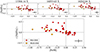 |
Fig. 22. [Nd/Fe] versus [Fe/H] for 50 M giants in our sample. The arrangement of the figures and markers is similar to Fig. 1. |
Mean s-process. In Fig. 23, we plot the mean abundances of the three s-process dominated elements, Y, Ce, and Nd, versus the metallicity. One can see that the three elements show star-by-star similarities. For example, the four stars at −0.4 < [Fe/H] < 0.0 marked in black in the figure all show high abundances of these s-process elements at the same time (part of the broader distribution of s-process abundances for a given metallicity; referred as the “cloud” earlier).
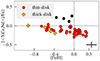 |
Fig. 23. Mean abundances of the three s-process elements, Y, Ce, and Nd, versus [Fe/H] for 50 M giants in our sample. Black filled circles represent the stars that show high abundances of all these s-process elements at the same time. The remaining markers are similar to Fig. 1. |
We show that these stars exhibit the same pattern (i.e., have relatively higher [s/Fe] abundances for all three elements obtained from different lines and different atomic data) in order to highlight the precision of the determined s-process abundances. Indeed, the thick-disk stars all follow the lower envelope of the thin disk in the same way for all these elements, too. It is worthwhile to note that these four stars with relatively higher [s/Fe] abundances are not abnormally high, as seen in Sect. 5.1.3 and Fig. 27, where the four stars were found within the s-process-cerium scatter “cloud”. The point here is rather that they exhibit a similar pattern in [Y,Ce,Nd/Fe], as explained above.
4.6.3. Element with 50/50 s- and r-process contributions (Yb)
Ytterbium. The ytterbium abundance was measured from the singly-ionized ytterbium line (Yb II) in the H-band at 16 498.40 Å. This line is severely blended with a CO molecular absorption line. In cool M giant spectra, the molecular absorption lines get stronger, and a careful analysis of the Yb line has to be carried out in order to retrieve a reliable elemental abundance from such a blended line (see discussion in Montelius et al. 2022). We made sure that the nearby CO lines from the same vibrational band were well fitted by the synthetic spectrum while determining the Yb abundances (for example, see Fig. A.5). This gave us confidence in the [Yb/Fe] abundance we determined from this difficult line. This is the first time that [Yb/Fe] has been determined from cool M giants in the −1.0 dex < [Fe/H] < 0.3 dex metallicity range.
There is a large scatter (∼0.5 dex) in the [Yb/Fe] values (see Fig. 24). However, this agrees well with the trend and scatter derived by Montelius et al. (2022) from warmer stars, which in general show weaker CO blending with the Yb line. Although there is a large scatter, the general picture that the thick-disk and the thin-disk [Yb/Fe] values more or less overlap is very similar to what Forsberg (2023) found for another 50/50 s- and r-process element, namely, praseodymium (Pr). Forsberg (2023) shows clearly in her study of ten s- and r-process elements with differing contributions of the two processes that the thick-disk trend goes from lying below the thin-disk trend for a “pure” s-process element (e.g., Ce) to the thick-disk trend lying above the thin-disk trend for a “pure” r-process element (e.g., Eu). The thick-disk trends for the elements with more equal mixtures of the two origins tend to lie between these extremes, which we observed here for Yb, reassuring us of the quality of the abundances large scatter in the [Yb/Fe] values.
 |
Fig. 24. [Yb/Fe] versus [Fe/H] for 49 M giants in our sample. The arrangement of the figures and markers is similar to Fig. 1. |
5. Discussion
5.1. Comparison with other studies
In the previous section, we presented detailed abundance trends of the 21 elements. Next, we needed to compare and validate the abundance trends of these elements with the abundance trends from other studies. First, we compared the abundance trends of 44 of our stars that were also observed in APOGEE with the abundances provided by the APOGEE DR17 catalog (Abdurro’uf et al. 2022). We also compared our abundance trends for all 50 stars with the abundance trends of six elements with weaker and blended spectral features for ∼19 000 cool stars (Teff < 4000 K) from APOGEE determined using the BACCHUS code in Hayes et al. (2022). Finally, we compared our trends with the abundance trends of ∼500 stars from the GILD sample (Jönsson et al., in prep., which builds upon and improves the analysis described in Jönsson et al. 2017), for which the stellar parameters and abundances have been determined from optical FIES spectra. For ytterbium, we compared our trend with the ytterbium abundances determined from the same line in the IGRINS H-band spectra of K giants in Montelius et al. (2022).
5.1.1. Comparison with APOGEE solar neighborhood stars
The APOGEE Survey team determined stellar parameters and elemental abundances for the 44 stars in common between our sample and that of APOGEE. However, abundances of only 11 elements are provided in the DR17 catalog for these cool stars, and none of the s-process elements are provided for these cool stars.
We used APOGEE’s spectroscopic values for the elemental abundances, not the calibrated ones, since the spectroscopic values are determined directly from the spectra, which is the same approach we used in this work, making the comparison more relevant. In Fig. 25, we plot the one-to-one elemental abundances with respect to hydrogen ([X/H]), including metallicity and 11 elements, determined from IGRINS spectra versus those in the APOGEE DR17 catalog for stars in common between APOGEE and this work. The mean difference determined for each element is also listed in the corresponding panels in the figure. We note that even though these stars observed by APOGEE and IGRINS are the same, the stellar parameters are different since we determined our own parameters and APOGEE also provides their own (for a comparison, see Paper I). Another obvious difference is that APOGEE’s spectral resolution is R = 22 500, whereas the IGRINS resolution is twice that.
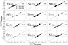 |
Fig. 25. Elemental abundances with respect to hydrogen ([X/H]) including metallicity and 11 elements determined from IGRINS spectra versus those in the APOGEE DR17 catalog for stars in common between APOGEE and this work. The black open circles and black open diamonds represent stars chemically classified as thin- and thick-disks, respectively, in our sample. The number of stars with valid APOGEE abundance estimates for each element are listed within the brackets in each panel. The linear one-to-one relation is shown by the black dashed line, and the mean difference values in metallicity and elemental abundances between this work and APOGEE are listed in the top-right part of each panel. |
As indicated by the numbers listed within the brackets in each panel of Fig. 25, APOGEE does not provide valid abundances for all 44 stars in our sample. It is also clear from Fig. 25 and the mean difference values that our abundance estimates are consistent with APOGEE for all elements except aluminum, potassium, chromium, and cobalt. For these elements, we found consistently lower values as compared to those of APOGEE.
The offset in abundances in this work with respect to APOGEE may be attributed to a combination of different factors, such as differences in spectral resolution, line selection, line lists, and pipelines between APOGEE and this work. Furthermore, in his comparative study analyzing APOGEE and the higher-resolution IGRINS spectra, Fridén (2023) showed that, in general, a higher spectral resolution helps in the analysis of stars at the metal-poor ends (for Ti, V, and Co) and metal-rich ends of trends. The higher resolution also yielded a tighter trend for the neutron-capture element Ce that followed the optical trend more closely.
5.1.2. Comparison with BAWLAS
Hayes et al. (2022) reanalyzed 126 000 APOGEE DR17 spectra of giants with a high signal-to-noise with the BACCHUS code. They provided abundances from the BACCHUS Analysis of Weak Lines in APOGEE Spectra (BAWLAS) catalog. The goal was to be able to use weaker and blended spectral features that the automated and rigid APOGEE pipeline cannot handle as well. Since they took special care of weaker lines and treated blends and upper limits, they were able to determine more precise abundances for Na, S, V, and Ce as a complement to the abundances given by the APOGEE pipeline. Furthermore, they also measured elements that APOGEE was unable to measure, such as P, Cu, and Nd. Similar to APOGEE DR17, chemical abundances derived for the above-mentioned elements were also calibrated to the respective solar zero-point derived from the solar neighborhood samples in the catalog. Capitalizing on very high-quality data, Hayes et al. (2022) thus showed that more information can be extracted from surveys when a well-chosen sub-sample is reanalyzed. In Fig. 26, we show the trends for six elements (Na, S, V, Cu, Ce, and Nd) determined in the BAWLAS study (Hayes et al. 2022) for ∼19 000 stars with Teff less than 4000 K in gray inverted triangles and our stars in red filled circles and orange diamonds.
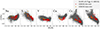 |
Fig. 26. Abundance trends versus metallicity of six elements determined for M giants in our sample (red filled circles and orange diamonds) and for ∼19 000 cool (Teff < 4000 K) giants (gray diamonds) from APOGEE DR17 reanalyzed using the BACCHUS code (Hayes et al. 2022). |
We used the same lines employed by Hayes et al. (2022) to derive abundances for Na and Nd, though we astrophysically updated the log gf-values for the Na lines and adopted log gf-values from Hasselquist et al. (2016) for Nd. For both Na and Nd, Hayes et al. (2022) calibrated their abundances with average zero-point offsets (with respect to the solar abundances in Grevesse et al. 2007) of ∼0.2 dex and ∼0.3 dex, respectively. Yet, our abundance trends are consistent with the BAWLAS abundance trends for Na and Nd.
Our abundance trends for the rest of the four elements lie either on the upper envelope (for S) or the lower envelope (for V, Cu, and Ce) of the BAWLAS abundances trends. One plausible explanation for this could be that for these four elements, we have used different lines or only a subset of lines from Hayes et al. (2022). In addition, we have updated the log gf-values astrophysically for certain elements (see Sect. 3.2), while zero-point offsets have been made to abundances as listed in Table 2 in Hayes et al. (2022).
5.1.3. Comparison with GILD
In Fig. 27, we plot the abundances determined for the 21 elements of the 50 solar neighborhood stars (red circles and orange diamonds) based on IGRINS spectra and the GILD sample (gray diamonds). While in the GILD project, high-resolution optical spectra of K giants were analyzed, in the IGRINS project, we analyzed high-resolution H- and K-band spectra of M giants, which are cooler. This means that there are no GILD stars that are in common with our IGRINS sample. GILD provides abundances for all elements in this study except fluorine, sulfur, and potassium. We compare the abundance trends of each group of elements (α, odd-Z, iron-peak, and neutron-capture) in the following paragraphs.
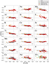 |
Fig. 27. Abundance trends versus metallicity of 21 elements determined for the 50 M giants in this work (red filled circles and orange diamonds). Gray diamonds represent the abundances determined for ∼500 K giants in the solar neighborhood from optical FIES spectra for all elements except F, S, K, Zn, and Yb (the latter is compared to abundances from Montelius et al. 2022), which are provided in the GILD catalog. |
A comparison of the α-element abundance trends for our IGRINS sample with the GILD sample has already been carried out in Paper I. They found the trends to be consistent with respect to each individual elemental abundance trend. While the Si and Ca trends align well, the Mg trend in GILD (which is similar to the optical dwarf trend of Bensby et al. 2014) is significantly higher when compared to our IGRINS trend and to that of APOGEE. Why the near-infrared Mg trends are lower than the optical one needs further investigation, but one reason could be inaccurate NLTE corrections. The thin disk-thick disk dichotomy in the metal-poor regime is also evident for all three α-elements and Ti in both the GILD and IGRINS samples.
The abundance trends of the odd-Z elements, Na and Al, for the IGRINS sample are consistent with the GILD sample abundance trends. An increase in [Na/Fe] at super-solar metallicities and the plateau at sub-solar metallicities are evident in both samples. The IGRINS trend, though, shows a hint of a downward trend for the lowest metallicity star, resulting in an N-shaped trend. This N-shape is also seen in other optical trends, as mentioned earlier, including in that of Bensby et al. (2014). Similarly, the [Al/Fe] trends from both samples agree, except at the lowest metallicities (at [Fe/H] < − 0.5 dex), where the thick-disk stars in the GILD sample reach a plateau, while the IGRINS sample decreases for decreasing metallicities.
Among the eight iron-peak elements, all except chromium and manganese show significant differences between the thin- and thick-disk stars in both the GILD and IGRINS samples. The near-infrared [Sc/Fe] trend is more scattered than the optical one, but it still has a clear thin-thick disk separation. The IGRINS [V/Fe] trend is tighter but lower than that of GILD. This might indicate a normalization problem. The thin-disk [Co/Fe] trends in both samples also overlap. The flat [Cr/Fe] trend in the GILD sample is similar to the IGRINS sample, as a majority of the GILD stars have slightly sub-solar values, which is the case with the IGRINS sample. The [Mn/Fe] trends are different in slope and magnitude, but the optical GILD abundances are not corrected for departures from LTE. The [Ni/Fe] trends in both samples exhibit tight trends that increase slightly at super-solar metallicities, which could point to metallicity-dependent yields that perhaps come from production in weak s (similar to the trend we observed in copper).
When it comes to the s-elements, the [Cu/Fe] trend in the GILD sample is more scattered, with the lowest values for stars at −0.5 < [Fe/H] < 0.0 dex, and it increases at super-solar metallicities. The IGRINS sample exhibits a similar N-shaped trend, although the IGRINS trends is less scattered.
The Y and Ce trends in IGRINS and GILD are remarkably similar. This further indicates that our intrinsic line strengths for Y are relevant (see Sect. 3.2). The thick disk follows the lower envelope of the thin disk, and there is a cosmic scatter at −0.5 < [Fe/H] < 0.0 dex. The [Yb/Fe] trend is consistent with the [Yb/Fe] trend determined from the same H-band line in IGRINS spectra of K giants by Montelius et al. (2022), which also shows a large scatter. This scatter could, however, in some part be cosmic since the thick-disk stars lie as expected compared to the pure s-elements. The [Nd/Fe] trend is, in general, higher than the optical [Nd/Fe] trend and also has some stars with higher [Nd/Fe] similar to the few outliers in the GILD sample. One reason for this is a systematic offset due to uncertain intrinsic line strengths (log gf-values).
The line strengths from the VALD database (in the case of yttrium) or astrophysical log gf-values were adopted from previous studies of neutron-capture lines (see Sect. 4.6.2). Meanwhile, multiple absorption lines in optical spectra for Y, Ce, and Nd have very reliable line strengths determined from experimental methods and are commonly used in large-scale optical spectroscopic surveys such as GALAH. This could also be the reason for the slightly lower values of [Ce/Fe] in the IGRINS sample that mainly follow the lower values of the optical [Ce/Fe] trend.
This points out the necessity of having a better line list in H- and K-bands with reliable line strengths (preferably measured in the laboratory), accurate wavelengths, hyperfine splitting information, and broadening parameters. Such a line list is crucial in order to determine accurate abundances of the rare heavy elements in cool stars from high-resolution near-infrared spectra.
5.2. Overall trends and precision
From Fig. 27, one can see how the thick-disk abundance trends clearly lie above those of the thin disk for the α-elements as well as for the elements Al, K, Sc, Ti, V, Co, and Ni. In contrast, for all the s-process dominated elements (Y, Ce, and Nd), the thick-disk stars lie along the lower envelope of the thin-disk “cloud”. This kind of behavior is indeed expected based on Galactic chemical evolution models (see, e.g., Grisoni et al. 2020), where s-process elements behave differently as compared to elements that are synthesized on a fast timescale, such as the α-elements, the weak s-process elements, like Cu, and the r-process dominated elements, like Eu. In our case, Yb lies between these cases, with a 50/50 contribution from the s- and r-processes.
The precision of the abundances determined in this work are discussed in Paper I and Paper II. They estimated the abundance uncertainties in the range of ∼0.04–0.11 dex resulting from typical uncertainties in stellar parameters (±100 K in Teff, ±0.2 dex in log g, ±0.1 dex in [Fe/H], and ±0.1 km s−1 in ξmicro). However, it is interesting to observe the general scatter in the abundance trends that are well determined. The [Si/Fe] abundance trend is, for example, very tight and clearly derived with a very high precision, less than 0.05 dex. Also, the fact that the thick-disk trends align well in general is an indication of the high precision. In Fig. 23, we also observed, as one more example, that the four stars that show a high mean s-process contribution have different stellar parameters and abundances that were derived from totally different spectral lines. This gives us confidence in the precision of our results, and we believe that the scatter in the s-process thin-disk trends at −0.5 < [Fe/H] < 0.0 (the abundance “cloud”) are real and therefore of cosmic origin. This is also clearly seen in the GILD abundances that were derived from optical spectra of warmer stars (see Forsberg 2023).
6. Conclusions
We have demonstrated that it is possible to retrieve 21 reliable abundance trends versus metallicity, namely for F, Mg, Si, S, Ca, Na, Al, K, Sc, Ti, V, Cr, Mn, Co, Ni, Cu, Zn, Y, Ce, Nd, and Yb, from high-resolution H- and K-band spectra, shown in this work with IGRINS spectra of 50 solar neighborhood stars. Our trends can be used for a differential comparison with other stellar populations in order to avoid any systematic uncertainties.
The fact that we are able to investigate all these elements in near-infrared spectra is important, as near-infrared spectrometers are becoming available, and these instruments can observe the obscure parts of the Milky Way. We have placed an emphasis on M giants since these stars are the brightest giants and are needed in order to chemically characterize the heavily obscured parts of the Milky Way, such as the Galactic Center region, which includes the nuclear stellar disk (NSD) and the nuclear star cluster (NSC). In order to be able to investigate the chemical history of the entire Milky Way, the dust-obscured regions also need to be studied in detail.
Among the 21 elements we studied, there are several different nucleosynthetic channels that provide empirical data for the Galactic chemical evolution with different timescales. The extended dimensions that these different channels provide will also provide decisive means to determine differences between populations (see, e.g., Manea et al. 2023). With the trends determined from infrared spectra, the interesting and important dust-obscured stellar populations (e.g., in the Galactic Center) can now be investigated. The important neutron-capture elements, both s- and r-dominated elements, can therefore be measured reliably. The fact that we can obtain Cu, Ce, Nd, and Yb abundances from the H-band points to the necessity of performing a dedicated, and meticulous analysis of high-quality spectra, that is, in a similar way as done in Hayes et al. (2022). In our case, we also provide an advance by observing at higher resolution, R ≥ 45 000, in order to even better disentangle blends and capture weak spectral features. Several K-band lines have been identified for F, Mg, Si, S, Ca, Na, Al, Sc, Ti, and Ni. The s-element Y can only be obtained from the K-band. While 21 elements are readily retrieved from IGRINS spectra, only 11 elements for these cool stars are provided in APOGEE. We note that the careful analysis of the BAWLAS study retrieved three extra elements.
Our trends agree well with other larger sets of data determined with proven methods from optical wavelengths. In our range of element trends, we observed clear similarities between groups of elements (such as the α-elements) and differences between others. The precision is high enough to also clearly separate the thick- and thin-disk trends for a wide variety of elements. We also confirm the increased cosmic scatter in the thin-disk s-process element trends for a given metallicity in the metallicity range of −0.5 < [Fe/H] < 0.0 (the abundance “cloud”). To our knowledge, there is no theoretical explanation for this increased abundance distribution for the given metallicities. We also clearly observed the “evolution” of the trends for the different neutron-capture elements from Cu to Yb via Y, Ce, and Nd, revealing the increasing r-process component of the elements’ origins. We also found a flat [Mn/Fe] versus [Fe/H] trend at low metallicities, implying that the NLTE grids used for optical and other types of stars might be relevant and correct.
Based on our findings, for future studies using near-infrared high-resolution spectroscopy, it is obvious that consistent NLTE corrections for the full parameter space as well as for more elements are needed, and the inconsistencies in abundance trends from different lines of the same element need to be further investigated. We also need more reliable line strengths and broadening parameters for near-infrared lines from experimental measurements and theoretical calculations.
Methods for deriving reliable stellar parameters and stellar abundances from high-resolution near-infrared spectra of M giants are also possible with instruments other than IGRINS. The GIANO and CRIRES+ spectrographs are available already, and in the near future, the MOONS spectrometer will be a workhorse, although at an APOGEE-type resolution. Future high-resolution near-infrared spectrometers projected for the extremely large telescopes, such as the ELT and TMT, will open up immense possibilities of observing more distant M giants, including in other galaxies.
Y-band at 0.95–1.1 μm; J-band at 1.1–1.4 μm; H-band at 1.5–1.8 μm; and K-band at 2.0–2.4 μm.
The signal-to-noise ratios were provided by RRISA (The Raw & Reduced IGRINS Spectral Archive; Sawczynec et al. 2022) and are the average S/N for the H- and K-bands, respectively, and is per resolution element. The S/N varies over the orders and is lowest at the ends of the orders.
Ramírez & Allende Prieto (2011) determined the fundamental parameters of Arcturus (or α Boo) as Teff = 4290 K, log g = 1.7, and [Fe/H] = −0.5 dex.
We refrain from providing a full line list with excitation energies, log gf, and broadening parameters since they are updated astrophysically and are hence model dependent.
Acknowledgments
We thank the anonymous referee for the constructive comments and suggestions that improved the quality of the paper. N.R. and G.N. are supported by the grant 2023-04744 from the Swedish Research Council. G.N. acknowledges the support from the Wenner-Gren Foundations (UPD2020-0191 and UPD2022-0059) and the Royal Physiographic Society in Lund through the Stiftelsen Walter Gyllenbergs fond. N.R. and R.F. acknowledge support from the Royal Physiographic Society in Lund through the Stiftelsen Walter Gyllenbergs fond and Märta och Erik Holmbergs donation. R.F. also acknowledges support from the Göran Gustafsson Foundation for Research in Natural Sciences and Medicine. M.M. acknowledges funding through VIDI grant “Pushing Galactic Archaeology to its limits” VI.Vidi.193.093, which is funded by the Dutch Research Council (NWO). G.M., H.J., B.T. acknowledge the financial support from the Wenner-Gren Foundation (WGF2022-0041). This work used The Immersion Grating Infrared Spectrometer (IGRINS) was developed under a collaboration between the University of Texas at Austin and the Korea Astronomy and Space Science Institute (KASI) with the financial support of the US National Science Foundation under grants AST-1229522, AST-1702267 and AST-1908892, McDonald Observatory of the University of Texas at Austin, the Korean GMT Project of KASI, the Mt. Cuba Astronomical Foundation and Gemini Observatory. This work is based on observations obtained at the international Gemini Observatory, a program of NSF’s NOIRLab, which is managed by the Association of Universities for Research in Astronomy (AURA) under a cooperative agreement with the National Science Foundation on behalf of the Gemini Observatory partnership: the National Science Foundation (United States), National Research Council (Canada), Agencia Nacional de Investigación y Desarrollo (Chile), Ministerio de Ciencia, Tecnología e Innovación (Argentina), Ministério da Ciência, Tecnologia, Inovações e Comunicações (Brazil), and Korea Astronomy and Space Science Institute (Republic of Korea). The following software and programming languages made this research possible: TOPCAT (version 4.6; Taylor et al. 2005); Python (version 3.8) and its packages ASTROPY (version 5.0; Astropy Collaboration 2022), SCIPY (Virtanen et al. 2020), MATPLOTLIB (Hunter 2007) and NUMPY (van der Walt et al. 2011).
References
- Abdurro’uf, Accetta, K., Aerts, C., et al. 2022, ApJS, 259, 35 [NASA ADS] [CrossRef] [Google Scholar]
- Aboussaïd, A., Carleer, M., Hurtmans, D., Biémont, E., & Godefroid, M. R. 1996, Phys. Scrip., 53, 28 [CrossRef] [Google Scholar]
- Afşar, M., Sneden, C., Frebel, A., et al. 2016, ApJ, 819, 103 [Google Scholar]
- Afşar, M., Sneden, C., Wood, M. P., et al. 2018, ApJ, 865, 44 [CrossRef] [Google Scholar]
- Afşar, M., Bozkurt, Z., Topcu, G. B., et al. 2023, ApJ, 949, 86 [CrossRef] [Google Scholar]
- Amarsi, A. M., Lind, K., Asplund, M., Barklem, P. S., & Collet, R. 2016, MNRAS, 463, 1518 [NASA ADS] [CrossRef] [Google Scholar]
- Amarsi, A. M., Nordlander, T., Barklem, P. S., et al. 2018, A&A, 615, A139 [NASA ADS] [CrossRef] [EDP Sciences] [Google Scholar]
- Amarsi, A. M., Nissen, P. E., & Skúladóttir, Á. 2019, A&A, 630, A104 [NASA ADS] [CrossRef] [EDP Sciences] [Google Scholar]
- Amarsi, A. M., Lind, K., Osorio, Y., et al. 2020, A&A, 642, A62 [EDP Sciences] [Google Scholar]
- Anstee, S. D., & O’Mara, B. J. 1991, MNRAS, 253, 549 [NASA ADS] [CrossRef] [Google Scholar]
- Anstee, S. D., & O’Mara, B. J. 1995, MNRAS, 276, 859 [Google Scholar]
- Arqueros, F. 1988, Opt. Commun., 67, 341 [NASA ADS] [CrossRef] [Google Scholar]
- Astropy Collaboration (Price-Whelan, A. M., et al.) 2022, ApJ, 935, 167 [NASA ADS] [CrossRef] [Google Scholar]
- Baratella, M., D’Orazi, V., Sheminova, V., et al. 2021, A&A, 653, A67 [NASA ADS] [CrossRef] [EDP Sciences] [Google Scholar]
- Barklem, P. S., & O’Mara, B. J. 1997, MNRAS, 290, 102 [Google Scholar]
- Barklem, P. S., O’Mara, B. J., & Ross, J. E. 1998, MNRAS, 296, 1057 [Google Scholar]
- Battistini, C., & Bensby, T. 2015, A&A, 577, A9 [NASA ADS] [CrossRef] [EDP Sciences] [Google Scholar]
- Battistini, C., & Bensby, T. 2016, A&A, 586, A49 [NASA ADS] [CrossRef] [EDP Sciences] [Google Scholar]
- Bensby, T., Feltzing, S., & Oey, M. S. 2014, A&A, 562, A71 [NASA ADS] [CrossRef] [EDP Sciences] [Google Scholar]
- Bergemann, M., & Gehren, T. 2008, A&A, 492, 823 [NASA ADS] [CrossRef] [EDP Sciences] [Google Scholar]
- Bergemann, M., Gallagher, A. J., Eitner, P., et al. 2019, A&A, 631, A80 [NASA ADS] [CrossRef] [EDP Sciences] [Google Scholar]
- Biemont, E., Quinet, P., & Zeippen, C. J. 1993, A&AS, 102, 435 [NASA ADS] [Google Scholar]
- Bisterzo, S., Travaglio, C., Gallino, R., Wiescher, M., & Käppeler, F. 2014, ApJ, 787, 10 [NASA ADS] [CrossRef] [Google Scholar]
- Böcek Topcu, G., Afşar, M., Sneden, C., et al. 2019, MNRAS, 485, 4625 [CrossRef] [Google Scholar]
- Böcek Topcu, G., Afşar, M., Sneden, C., et al. 2020, MNRAS, 491, 544 [CrossRef] [Google Scholar]
- Brady, K. E., Sneden, C., Pilachowski, C. A., et al. 2023, AJ, 166, 154 [CrossRef] [Google Scholar]
- Brooke, J. S. A., Bernath, P. F., Western, C. M., et al. 2016, J. Quant. Spectr. Rad. Transf., 168, 142 [NASA ADS] [CrossRef] [Google Scholar]
- Carr, J. S., Sellgren, K., & Balachandran, S. C. 2000, ApJ, 530, 307 [NASA ADS] [CrossRef] [Google Scholar]
- Chang, E. S. 1990, J. Phys. Chem. Ref. Data, 19, 119 [NASA ADS] [CrossRef] [Google Scholar]
- Cirasuolo, M., Afonso, J., Bender, R., et al. 2012, SPIE, 8446, 84460S [NASA ADS] [Google Scholar]
- Clayton, D. 2003, Handbook of Isotopes in the Cosmos (Cambridge University Press) [Google Scholar]
- Costa Silva, A. R., Delgado Mena, E., & Tsantaki, M. 2020, A&A, 634, A136 [EDP Sciences] [Google Scholar]
- Cowan, R. D. 1981, Phys. SCR, 24, 615 [NASA ADS] [CrossRef] [Google Scholar]
- Cunha, K., Sellgren, K., Smith, V. V., et al. 2007, ApJ, 669, 1011 [NASA ADS] [CrossRef] [Google Scholar]
- Cunha, K., Smith, V. V., Hasselquist, S., et al. 2017, ApJ, 844, 145 [Google Scholar]
- Curtis, S., Ebinger, K., Fröhlich, C., et al. 2019, ApJ, 870, 2 [Google Scholar]
- da Silveira, C. R., Barbuy, B., Friaça, A. C. S., et al. 2018, A&A, 614, A149 [NASA ADS] [CrossRef] [EDP Sciences] [Google Scholar]
- Delgado Mena, E., Tsantaki, M., Adibekyan, V. Z., et al. 2017, A&A, 606, A94 [NASA ADS] [CrossRef] [EDP Sciences] [Google Scholar]
- de los Reyes, M. A. C., Kirby, E. N., Seitenzahl, I. R., & Shen, K. J. 2020, ApJ, 891, 85 [NASA ADS] [CrossRef] [Google Scholar]
- Demarque, P., Woo, J.-H., Kim, Y.-C., & Yi, S. K. 2004, ApJS, 155, 667 [NASA ADS] [CrossRef] [Google Scholar]
- Ernandes, H., Barbuy, B., Friaça, A. C. S., et al. 2020, A&A, 640, A89 [NASA ADS] [CrossRef] [EDP Sciences] [Google Scholar]
- Ertmer, W., & Hofer, B. 1976, Zeitschrift fur Physik A Hadrons and Nuclei, 276, 9 [NASA ADS] [Google Scholar]
- Follert, R., Dorn, R. J., Oliva, E., et al. 2014, SPIE Conf. Ser., 9147, 914719 [Google Scholar]
- Forsberg, R. 2023, Ph.D. Thesis, Lund University, Sweden [Google Scholar]
- Forsberg, R., Jönsson, H., Ryde, N., & Matteucci, F. 2019, A&A, 631, A113 [NASA ADS] [CrossRef] [EDP Sciences] [Google Scholar]
- Fridén, E. 2023, PhD Thesis, Lund University, Sweden [Google Scholar]
- Frogel, J. A., Tiede, G. P., & Kuchinski, L. E. 1999, AJ, 117, 2296 [NASA ADS] [CrossRef] [Google Scholar]
- García-Hernández, D. A., Rao, N. K., Lambert, D. L., et al. 2023, ApJ, 948, 15 [CrossRef] [Google Scholar]
- Garro, E. R., Fernández-Trincado, J. G., Minniti, D., et al. 2023, A&A, 669, A136 [NASA ADS] [CrossRef] [EDP Sciences] [Google Scholar]
- Genoni, M., Riva, M., Pariani, G., Aliverti, M., & Moschetti, M. 2016, SPIE Conf. Ser., 9911, 99112L [Google Scholar]
- Gilmozzi, R., & Spyromilio, J. 2008, SPIE Conf. Ser., 7012, 701219 [NASA ADS] [Google Scholar]
- Grevesse, N., Asplund, M., & Sauval, A. J. 2007, Space. Sci. Rev., 130, 105 [NASA ADS] [CrossRef] [Google Scholar]
- Grevesse, N., Scott, P., Asplund, M., & Sauval, A. J. 2015, A&A, 573, A27 [CrossRef] [EDP Sciences] [Google Scholar]
- Grisoni, V., Romano, D., Spitoni, E., et al. 2020, MNRAS, 498, 1252 [NASA ADS] [CrossRef] [Google Scholar]
- Guerço, R., Ramírez, S., Cunha, K., et al. 2022, ApJ, 929, 24 [CrossRef] [Google Scholar]
- Gully-Santiago, M., Wang, W., Deen, C., & Jaffe, D. 2012, SPIE Conf. Ser., 8450, 84502S [NASA ADS] [Google Scholar]
- Gustafsson, B., Edvardsson, B., Eriksson, K., et al. 2008, A&A, 486, 951 [NASA ADS] [CrossRef] [EDP Sciences] [Google Scholar]
- Han, J. Y., Yuk, I. S., Ko, K., et al. 2012, SPIE Conf. Ser., 8550, 85501B [NASA ADS] [Google Scholar]
- Hasselquist, S., Shetrone, M., Cunha, K., et al. 2016, ApJ, 833, 81 [Google Scholar]
- Hayes, C. R., Masseron, T., Sobeck, J., et al. 2022, ApJS, 262, 34 [NASA ADS] [CrossRef] [Google Scholar]
- Hinkle, K., Wallace, L., & Livingston, W. 1995, PASP, 107, 1042 [Google Scholar]
- Holanda, N., Roriz, M. P., Drake, N. A., et al. 2024, MNRAS, 527, 1389 [Google Scholar]
- Hunter, J. D. 2007, Comput. Sci. Eng., 9, 90 [NASA ADS] [CrossRef] [Google Scholar]
- Ikeda, Y., Kobayashi, N., Kondo, S., et al. 2007, SPIE Conf. Ser., 9908, 99085Z [NASA ADS] [Google Scholar]
- Jeong, U., Chun, M. Y., Oh, J. S., et al. 2014, SPIE Conf. Ser., 9154, 91541X [NASA ADS] [Google Scholar]
- Jönsson, H., Ryde, N., Nordlander, T., et al. 2017, A&A, 598, A100 [NASA ADS] [CrossRef] [EDP Sciences] [Google Scholar]
- Jönsson, H., Holtzman, J. A., Allende Prieto, C., et al. 2020, AJ, 160, 120 [Google Scholar]
- Kaplan, K. F., Dinerstein, H. L., Oh, H., et al. 2017, ApJ, 838, 152 [CrossRef] [Google Scholar]
- Kaplan, K. F., Dinerstein, H. L., Kim, H., & Jaffe, D. T. 2021, ApJ, 919, 27 [NASA ADS] [CrossRef] [Google Scholar]
- Kobayashi, C., & Nakasato, N. 2011, ApJ, 729, 16 [NASA ADS] [CrossRef] [Google Scholar]
- Kobayashi, C., Karakas, A. I., & Lugaro, M. 2020, ApJ, 900, 179 [Google Scholar]
- Kupka, F. G., Ryabchikova, T. A., Piskunov, N. E., Stempels, H. C., & Weiss, W. W. 2000, Baltic Astron., 9, 590 [Google Scholar]
- Kurucz, R. L. 2006, Robert L. Kurucz online Database of Observed and Predicted Atomic Transitions [Google Scholar]
- Kurucz, R. L. 2008, Online Database of Observed and Predicted Atomic Transitions [Google Scholar]
- Lee, S., Lee, J.-E., Park, S., et al. 2016, ApJ, 826, 179 [NASA ADS] [CrossRef] [Google Scholar]
- Lee, J.-J., Gullikson, K., & Kaplan, K. 2017, https://doi.org/10.5281/zenodo.845059 [Google Scholar]
- Li, G., Gordon, I. E., Rothman, L. S., et al. 2015, ApJS, 216, 15 [NASA ADS] [CrossRef] [Google Scholar]
- Lim, D., Koch-Hansen, A. J., Chun, S.-H., Hong, S., & Lee, Y.-W. 2022, A&A, 666, A62 [NASA ADS] [CrossRef] [EDP Sciences] [Google Scholar]
- Lind, K., Amarsi, A. M., Asplund, M., et al. 2017, MNRAS, 468, 4311 [NASA ADS] [CrossRef] [Google Scholar]
- Lodders, K. 2003, ApJ, 591, 1220 [Google Scholar]
- Lomaeva, M., Jönsson, H., Ryde, N., Schultheis, M., & Thorsbro, B. 2019, A&A, 625, A141 [NASA ADS] [CrossRef] [EDP Sciences] [Google Scholar]
- López-Valdivia, R., Mace, G. N., Han, E., et al. 2023, ApJ, 943, 49 [CrossRef] [Google Scholar]
- Mace, G., Kim, H., Jaffe, D. T., et al. 2016 SPIE Conf. Ser., 9908, 99080C [NASA ADS] [Google Scholar]
- Mace, G., Sokal, K., Lee, J. J., et al. 2018, SPIE Conf. Ser., 10702, 107020Q [NASA ADS] [Google Scholar]
- Madonna, S., Bautista, M., Dinerstein, H. L., et al. 2018, ApJ, 861, L8 [NASA ADS] [CrossRef] [Google Scholar]
- Maiolino, R., Haehnelt, M., Murphy, M. T., et al. 2013, arXiv eprints [arXiv:1310.3163] [Google Scholar]
- Manea, C., Hawkins, K., Ness, M. K., et al. 2023, AAS J., submitted [arXiv:2310.15257] [Google Scholar]
- Mawet, D., Fitzgerald, M., Konopacky, Q., et al. 2019, Bull. Am. Astron. Soc., 51, 134 [Google Scholar]
- Mishenina, T. V., Kovtyukh, V. V., Soubiran, C., Travaglio, C., & Busso, M. 2002, A&A, 396, 189 [NASA ADS] [CrossRef] [EDP Sciences] [Google Scholar]
- Montelius, M. 2021, Towards a High Resolution View of Infrared Line Formation (Student Paper) [Google Scholar]
- Montelius, M., Forsberg, R., Ryde, N., et al. 2022, A&A, 665, A135 [NASA ADS] [CrossRef] [EDP Sciences] [Google Scholar]
- Moon, B., Wang, W., Park, C., et al. 2012, SPIE Conf. Ser., 8450, 845048 [NASA ADS] [Google Scholar]
- Nandakumar, G., Ryde, N., Schultheis, M., et al. 2018, MNRAS, 478, 4374 [Google Scholar]
- Nandakumar, G., Ryde, N., Casagrande, L., & Mace, G. 2023a, A&A, 675, A23 [NASA ADS] [CrossRef] [EDP Sciences] [Google Scholar]
- Nandakumar, G., Ryde, N., & Mace, G. 2023b, A&A, 676, A79 [NASA ADS] [CrossRef] [EDP Sciences] [Google Scholar]
- Nieuwmunster, N., Nandakumar, G., Spitoni, E., et al. 2023, A&A, 671, A94 [NASA ADS] [CrossRef] [EDP Sciences] [Google Scholar]
- Nordlander, T., & Lind, K. 2017, A&A, 607, A75 [NASA ADS] [CrossRef] [EDP Sciences] [Google Scholar]
- Oh, J. S., Park, C., Cha, S. M., et al. 2014, SPIE Conf. Ser., 9147, 914739 [NASA ADS] [Google Scholar]
- Origlia, L., Oliva, E., Baffa, C., et al. 2014, SPIE Conf. Ser., 9147, 91471E [Google Scholar]
- Park, C., Jaffe, D. T., Yuk, I. S., et al. 2014, SPIE Conf. Ser., 9147, 91471D [NASA ADS] [Google Scholar]
- Park, S., Lee, J.-E., Kang, W., et al. 2018, ApJS, 238, 29 [Google Scholar]
- Pehlivan, A., Nilsson, H., & Hartman, H. 2015, A&A, 582, A98 [NASA ADS] [CrossRef] [EDP Sciences] [Google Scholar]
- Perdigon, J., de Laverny, P., Recio-Blanco, A., et al. 2021, A&A, 647, A162 [NASA ADS] [CrossRef] [EDP Sciences] [Google Scholar]
- Pignatari, M., Gallino, R., Heil, M., et al. 2010, ApJ, 710, 1557 [Google Scholar]
- Piskunov, N. E., Kupka, F., Ryabchikova, T. A., Weiss, W. W., & Jeffery, C. S. 1995, A&AS, 112, 525 [Google Scholar]
- Prantzos, N., Abia, C., Limongi, M., Chieffi, A., & Cristallo, S. 2018, MNRAS, 476, 3432 [Google Scholar]
- Prantzos, N., Abia, C., Cristallo, S., Limongi, M., & Chieffi, A. 2020, MNRAS, 491, 1832 [Google Scholar]
- Ramírez, I., & Allende Prieto, C. 2011, ApJ, 743, 135 [Google Scholar]
- Ramírez, S. V., Stephens, A. W., Frogel, J. A., & DePoy, D. L. 2000, AJ, 120, 833 [CrossRef] [Google Scholar]
- Rich, R. M., Origlia, L., & Valenti, E. 2007, ApJ, 665, L119 [NASA ADS] [CrossRef] [Google Scholar]
- Rich, R. M., Origlia, L., & Valenti, E. 2012, ApJ, 746, 59 [NASA ADS] [CrossRef] [Google Scholar]
- Ryabchikova, T., Piskunov, N., Kurucz, R. L., et al. 2015, Phys. SCR, 90, 054005 [NASA ADS] [CrossRef] [Google Scholar]
- Ryde, N., & Schultheis, M. 2015, A&A, 573, A14 [NASA ADS] [CrossRef] [EDP Sciences] [Google Scholar]
- Ryde, N., Fritz, T. K., Rich, R. M., et al. 2016a, ApJ, 831, 40 [Google Scholar]
- Ryde, N., Schultheis, M., Grieco, V., et al. 2016b, AJ, 151, 1 [Google Scholar]
- Sales-Silva, J. V., Daflon, S., Cunha, K., et al. 2022, ApJ, 926, 154 [NASA ADS] [CrossRef] [Google Scholar]
- Sawczynec, E., Mace, G., Gully-Santiago, M., & Jaffe, D. 2022, Am. Astron. Soc. Meeting Abstracts, 54, 20306 [Google Scholar]
- Skidmore, W., Bernstein, R., Dumas, C., et al. 2022, J. Astron. Telescopes Instrum. Syst., 8, 021510 [NASA ADS] [Google Scholar]
- Sneden, C., Lucatello, S., Ram, R. S., Brooke, J. S. A., & Bernath, P. 2014, ApJS, 214, 26 [Google Scholar]
- Sneden, C., Cowan, J. J., Kobayashi, C., et al. 2016, ApJ, 817, 53 [NASA ADS] [CrossRef] [Google Scholar]
- Sterling, N. C., Dinerstein, H. L., Kaplan, K. F., & Bautista, M. A. 2016, ApJ, 819, L9 [NASA ADS] [CrossRef] [Google Scholar]
- Takeda, Y. 2019, Stars and Galaxies, 2, 1 [NASA ADS] [Google Scholar]
- Takeda, Y., Zhao, G., Chen, Y.-Q., Qiu, H.-M., & Takada-Hidai, M. 2002, PASJ, 54, 275 [NASA ADS] [CrossRef] [Google Scholar]
- Tamai, R., & Spyromilio, J. 2014, SPIE Conf. Ser., 9145, 91451E [NASA ADS] [Google Scholar]
- Tautvaišienė, G., Viscasillas Vázquez, C., Mikolaitis, Š., et al. 2021, A&A, 649, A126 [NASA ADS] [CrossRef] [EDP Sciences] [Google Scholar]
- Taylor, M. B. 2005, ASP Conf. Ser., 347, 29 [Google Scholar]
- Thorsbro, B., Ryde, N., Schultheis, M., et al. 2018, ApJ, 866, 52 [NASA ADS] [CrossRef] [Google Scholar]
- Tody, D. 1993, ASP Conf. Ser., 52, 173 [NASA ADS] [Google Scholar]
- Valenti, J. A., & Piskunov, N. 1996, A&AS, 118, 595 [NASA ADS] [CrossRef] [EDP Sciences] [Google Scholar]
- Valenti, J. A., & Piskunov, N. 2012, Astrophysics Source Code Library [record ascl: 1202.013] [Google Scholar]
- van der Walt, S., Colbert, S. C., & Varoquaux, G. 2011, Comput. Sci. Eng., 13, 22 [Google Scholar]
- Vasini, A., Spitoni, E., & Matteucci, F. 2024, A&A, 683, A121 [NASA ADS] [CrossRef] [EDP Sciences] [Google Scholar]
- Virtanen, P., Gommers, R., Oliphant, T. E., et al. 2020, Nat. Methods, 17, 261 [Google Scholar]
- Wallace, L., & Livingston, W. 2003, An atlas of the solar spectrum in the infrared from 1850 to 9000 cm-1 (1.1 to 5.4 micrometer) (Tucson: National Solar Observatory, National Optical Astronomy Observatory), NSO Technical Report [Google Scholar]
- Wang, W., Gully-Santiago, M., Deen, C., Mar, D. J., & Jaffe, D. T. 2010, SPIE Conf. Ser., 7739, 77394L [NASA ADS] [Google Scholar]
- Woosley, S. E., & Weaver, T. A. 1995, ApJS, 101, 181 [Google Scholar]
- Yuk, I. S., Jaffe, D. T., Barnes, S., et al. 2010, SPIE Conf. Ser., 7735, 77351M [NASA ADS] [Google Scholar]
- Zasowski, G., Schultheis, M., Hasselquist, S., et al. 2019, ApJ, 870, 138 [NASA ADS] [CrossRef] [Google Scholar]
Appendix A: Additional figures
 |
Fig. A.1. Wavelength regions centered at the five selected fluorine lines for the star 2M18103303-1626220 (star 41). In each panel, the black circles denote the observed spectrum, the crimson line denotes the best-fit synthetic spectrum, and the red band denotes the variation in the synthetic spectrum for a difference of ±0.2 dex in the [F/Fe]. The yellow bands in each panel represent the line masks defined for the F lines, wherein SME fits observed spectra by varying the fluorine abundance and finds the best synthetic spectra fit by χ2 minimization. The green line shows the synthetic spectrum without F, also indicating any possible blends in the line, and the orange line shows the telluric spectrum of the standard star that is used to correct for telluric contaminations in the observed star spectrum. The [F/Fe] values corresponding to the best-fit case for each F line are listed in each panel. All identified atomic and molecular lines are also denoted at the top of each panel. |
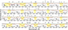 |
Fig. A.2. Alpha elements. The wavelength regions are centered at the three selected magnesium lines for the star 2M05594446-7212111 (star 2), at the four selected silicon lines for the star 2M06074096-0530332 (star 6), at the two selected sulfur lines for the star 2M14131192-4849280 (star 20), and at the 11 selected calcium lines for the star 2M14240039-6252516 (star 21). Arrangement of figures and plot descriptions are similar to Figure A.1. |
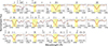 |
Fig. A.3. Odd-Z elements. The wavelength regions are centered at the five selected sodium lines (we note that only the two H-band lines were used to estimate the mean [Na/Fe] in Figure 6) for the star 2M06052796-0553384 (star 5), at the seven selected aluminum lines for the star 2M14275833-6147534 (star 25), and at the two selected potassium lines for the star 2M13403516-5040261 (star 19). Arrangement of figures and plot descriptions are similar to Figure A.1. |
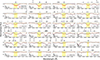 |
Fig. A.4. Iron-peak elements and zinc. The wavelength regions are centered at the three selected scandium lines for the star 2M14131192-4849280 (star 20), at the two selected titanium lines for the star 2M06223443-0443153 (star 11), at the one selected vanadium line for the star 2M06171159-7259319 (star 10), at the three selected chromium lines for the star 2M14371958-6251344 (star 37), at the two selected manganese lines for the star 2M06143705-0551064 (star 9), at the one selected chromium line for the star 2M14345114-6225509 (star 34), at the 11 selected nickel lines for the star 2M18103303-1626220 (star 41), and at the one selected zinc line for the star 2M14332869-6211255 (star 31). Arrangement of figures and plot descriptions are similar to Figure A.1. |
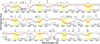 |
Fig. A.5. Neutron-capture elements. The wavelength regions are centered at the two selected copper lines for the star 2M14360935-6309399 (star 36), at the two selected yttrium lines for the star 2M14261117-6240220 (star 24), at the four selected cerium lines for the star 2M06574070-1231239 (star 15), at the three selected neodymium lines for the star 2M13403516-5040261 (star 19), and at the one selected ytterbium line for the star 2M05484106-0602007 (star 1). Arrangement of figures and plot descriptions are similar to Figure A.1. |
All Figures
|
Fig. 1. [F/Fe] versus [Fe/H] trends for 50 M giants in our sample. Figures in the upper panel show the trends determined from five individual HF lines. The mean [F/Fe] versus [Fe/H] trend from all six lines is shown in the bottom panel. Red filled circles and orange diamonds denote the thin- and thick-disk stars, respectively. The error bar in the bottom-right part of the top panels and the bottom panel indicate the uncertainties in abundances determined from each line and the mean uncertainty determined as the standard error of mean (see text in the Sect. 4 for more details). |
| In the text | |
|
Fig. 2. [Mg/Fe] versus [Fe/H] for 50 M giants in our sample. The arrangement of the figures and markers is similar to Fig. 1. |
| In the text | |
|
Fig. 3. [Si/Fe] versus [Fe/H] for 50 M giants in our sample. The arrangement of the figures and markers is similar to Fig. 1. |
| In the text | |
|
Fig. 4. [S/Fe] versus [Fe/H] for 48 M giants in our sample. The arrangement of the figures and markers is similar to Fig. 1. |
| In the text | |
|
Fig. 5. [Ca/Fe] versus [Fe/H] for 50 M giants in our sample. The arrangement of the figures and markers is similar to Fig. 1. |
| In the text | |
|
Fig. 6. [Na/Fe] versus [Fe/H] for 50 M giants in our sample. The arrangement of the figures and markers is similar to Fig. 1. We exclude [Na/Fe] abundances from the three K-band lines to estimate the mean [Na/Fe] abundance since the abundances from these lines are sub-solar for the sub-solar metallicity stars. This is inconsistent with the abundances from H-band lines, as well as in APOGEE and other optical studies (see also Figs. 25–27). |
| In the text | |
|
Fig. 7. NLTE-LTE differences versus [Fe/H] for sodium (Na) abundances from the two H-band and three K-band lines for 50 M giants in our sample. NLTE corrections are higher and ranges from ∼ − 0.4 dex to ∼ − 0.1 dex for the K-band lines. |
| In the text | |
|
Fig. 8. [Al/Fe] versus [Fe/H] for 50 M giants in our sample. The arrangement of the figures and markers is similar to Fig. 1. |
| In the text | |
|
Fig. 9. [K/Fe] versus [Fe/H] for 48 M giants in our sample. The arrangement of the figures and markers is similar to Fig. 1. |
| In the text | |
|
Fig. 10. [Sc/Fe] versus [Fe/H] for 50 M giants in our sample. The arrangement of the figures and markers is similar to Fig. 1. |
| In the text | |
|
Fig. 11. [Ti/Fe] versus [Fe/H] for 50 M giants in our sample. The arrangement of the figures and markers is similar to Fig. 1. |
| In the text | |
|
Fig. 12. [V/Fe] versus [Fe/H] for 50 M giants in our sample. The arrangement of the figures and markers is similar to Fig. 1. |
| In the text | |
|
Fig. 13. [Cr/Fe] versus [Fe/H] for 50 M giants in our sample. The arrangement of the figures and markers is similar to Fig. 1. |
| In the text | |
|
Fig. 14. [Mn/Fe] versus [Fe/H] for 50 M giants in our sample. The arrangement of the figures and markers is similar to Fig. 1. |
| In the text | |
|
Fig. 15. Manganese abundance trends and NLTE-LTE differences as a function of [Fe/H] for 50 M giants in this work and 38 K giants in Montelius (2021). Upper panel: [Mn/Fe] versus [Fe/H] for solar neighborhood M giants in this work (filled circles) and for the warmer K giants (Teff > 4000 K) analyzed in Montelius (2021) (inverted triangles) color coded in Teff and including the NLTE corrections and determined from the same H-band lines. Bottom panel: NLTE corrections (NLTE-LTE) to manganese abundances based on the calculations by Amarsi et al. (2020) for M giants in this work and K giants analyzed in Montelius (2021). Markers are the same as in the upper panel. The NLTE corrections for the abundance derived from these lines depend on the effective temperatures of the stars. |
| In the text | |
|
Fig. 16. [Co/Fe] versus [Fe/H] for 50 M giants in our sample. The arrangement of the figures and markers is similar to Fig. 1. |
| In the text | |
|
Fig. 17. [Ni/Fe] versus [Fe/H] for 50 M giants in our sample. The arrangement of the figures and markers is similar to Fig. 1. |
| In the text | |
|
Fig. 18. [Zn/Fe] versus [Fe/H] for 35 M giants in our sample. The arrangement of the figures and markers is similar to Fig. 1. |
| In the text | |
|
Fig. 19. [Cu/Fe] versus [Fe/H] for 36 M giants in our sample. The arrangement of the figures and markers is similar to Fig. 1. |
| In the text | |
|
Fig. 20. [Y/Fe] versus [Fe/H] for 50 M giants in our sample. The arrangement of the figures and markers is similar to Fig. 1. |
| In the text | |
|
Fig. 21. [Ce/Fe] versus [Fe/H] for 50 M giants in our sample. The arrangement of the figures and markers is similar to Fig. 1. |
| In the text | |
|
Fig. 22. [Nd/Fe] versus [Fe/H] for 50 M giants in our sample. The arrangement of the figures and markers is similar to Fig. 1. |
| In the text | |
|
Fig. 23. Mean abundances of the three s-process elements, Y, Ce, and Nd, versus [Fe/H] for 50 M giants in our sample. Black filled circles represent the stars that show high abundances of all these s-process elements at the same time. The remaining markers are similar to Fig. 1. |
| In the text | |
|
Fig. 24. [Yb/Fe] versus [Fe/H] for 49 M giants in our sample. The arrangement of the figures and markers is similar to Fig. 1. |
| In the text | |
|
Fig. 25. Elemental abundances with respect to hydrogen ([X/H]) including metallicity and 11 elements determined from IGRINS spectra versus those in the APOGEE DR17 catalog for stars in common between APOGEE and this work. The black open circles and black open diamonds represent stars chemically classified as thin- and thick-disks, respectively, in our sample. The number of stars with valid APOGEE abundance estimates for each element are listed within the brackets in each panel. The linear one-to-one relation is shown by the black dashed line, and the mean difference values in metallicity and elemental abundances between this work and APOGEE are listed in the top-right part of each panel. |
| In the text | |
|
Fig. 26. Abundance trends versus metallicity of six elements determined for M giants in our sample (red filled circles and orange diamonds) and for ∼19 000 cool (Teff < 4000 K) giants (gray diamonds) from APOGEE DR17 reanalyzed using the BACCHUS code (Hayes et al. 2022). |
| In the text | |
|
Fig. 27. Abundance trends versus metallicity of 21 elements determined for the 50 M giants in this work (red filled circles and orange diamonds). Gray diamonds represent the abundances determined for ∼500 K giants in the solar neighborhood from optical FIES spectra for all elements except F, S, K, Zn, and Yb (the latter is compared to abundances from Montelius et al. 2022), which are provided in the GILD catalog. |
| In the text | |
|
Fig. A.1. Wavelength regions centered at the five selected fluorine lines for the star 2M18103303-1626220 (star 41). In each panel, the black circles denote the observed spectrum, the crimson line denotes the best-fit synthetic spectrum, and the red band denotes the variation in the synthetic spectrum for a difference of ±0.2 dex in the [F/Fe]. The yellow bands in each panel represent the line masks defined for the F lines, wherein SME fits observed spectra by varying the fluorine abundance and finds the best synthetic spectra fit by χ2 minimization. The green line shows the synthetic spectrum without F, also indicating any possible blends in the line, and the orange line shows the telluric spectrum of the standard star that is used to correct for telluric contaminations in the observed star spectrum. The [F/Fe] values corresponding to the best-fit case for each F line are listed in each panel. All identified atomic and molecular lines are also denoted at the top of each panel. |
| In the text | |
|
Fig. A.2. Alpha elements. The wavelength regions are centered at the three selected magnesium lines for the star 2M05594446-7212111 (star 2), at the four selected silicon lines for the star 2M06074096-0530332 (star 6), at the two selected sulfur lines for the star 2M14131192-4849280 (star 20), and at the 11 selected calcium lines for the star 2M14240039-6252516 (star 21). Arrangement of figures and plot descriptions are similar to Figure A.1. |
| In the text | |
|
Fig. A.3. Odd-Z elements. The wavelength regions are centered at the five selected sodium lines (we note that only the two H-band lines were used to estimate the mean [Na/Fe] in Figure 6) for the star 2M06052796-0553384 (star 5), at the seven selected aluminum lines for the star 2M14275833-6147534 (star 25), and at the two selected potassium lines for the star 2M13403516-5040261 (star 19). Arrangement of figures and plot descriptions are similar to Figure A.1. |
| In the text | |
|
Fig. A.4. Iron-peak elements and zinc. The wavelength regions are centered at the three selected scandium lines for the star 2M14131192-4849280 (star 20), at the two selected titanium lines for the star 2M06223443-0443153 (star 11), at the one selected vanadium line for the star 2M06171159-7259319 (star 10), at the three selected chromium lines for the star 2M14371958-6251344 (star 37), at the two selected manganese lines for the star 2M06143705-0551064 (star 9), at the one selected chromium line for the star 2M14345114-6225509 (star 34), at the 11 selected nickel lines for the star 2M18103303-1626220 (star 41), and at the one selected zinc line for the star 2M14332869-6211255 (star 31). Arrangement of figures and plot descriptions are similar to Figure A.1. |
| In the text | |
|
Fig. A.5. Neutron-capture elements. The wavelength regions are centered at the two selected copper lines for the star 2M14360935-6309399 (star 36), at the two selected yttrium lines for the star 2M14261117-6240220 (star 24), at the four selected cerium lines for the star 2M06574070-1231239 (star 15), at the three selected neodymium lines for the star 2M13403516-5040261 (star 19), and at the one selected ytterbium line for the star 2M05484106-0602007 (star 1). Arrangement of figures and plot descriptions are similar to Figure A.1. |
| In the text | |
Current usage metrics show cumulative count of Article Views (full-text article views including HTML views, PDF and ePub downloads, according to the available data) and Abstracts Views on Vision4Press platform.
Data correspond to usage on the plateform after 2015. The current usage metrics is available 48-96 hours after online publication and is updated daily on week days.
Initial download of the metrics may take a while.