| Issue |
A&A
Volume 671, March 2023
|
|
|---|---|---|
| Article Number | A94 | |
| Number of page(s) | 18 | |
| Section | Galactic structure, stellar clusters and populations | |
| DOI | https://doi.org/10.1051/0004-6361/202245374 | |
| Published online | 08 March 2023 | |
Detailed α abundance trends in the inner Galactic bulge
1
Université Côte d’Azur, Observatoire de la Côte d’Azur, Laboratoire Lagrange, CNRS, Blvd de l’Observatoire, 06304 Nice, France
e-mail: This email address is being protected from spambots. You need JavaScript enabled to view it.
2
Lund Observatory, Department of Astronomy and Theoretical Physics, Lund University, Box 43 22100 Lund, Sweden
3
Stellar Astrophysics Centre, Department of Physics and Astronomy, Aarhus University, Ny Munkegade 120, 8000 Aarhus C, Denmark
4
Department of Physics and Astronomy, UCLA, 430 Portola Plaza, Box 951547 Los Angeles, CA 90095-1547, USA
5
Theoretical Astrophysics, Department of Physics and Astronomy, Uppsala University, Box 516 751 20 Uppsala, Sweden
6
Dipartimento di Fisica, Sezione di Astronomia, Università di Trieste, Via G.B. Tiepolo 11, 34131 Trieste, Italy
7
I.N.A.F. Osservatorio Astronomico di Trieste, Via G.B. Tiepolo 11, 34131 Trieste, Italy
8
I.N.F.N. Sezione di Trieste, Via Valerio 2, 34134 Trieste, Italy
Received:
4
November
2022
Accepted:
9
January
2023
Abstract
Context. Until now, heavy interstellar extinction has meant that only a few studies of chemical abundances have been possible in the inner Galactic bulge. However, it is crucial to learn more about this structure in order to better understand the formation and evolution of the centre of the Galaxy and galaxies in general.
Aims. In this paper, we aim to derive high-precision α-element abundances using CRIRES high-resolution IR spectra of 72 cool M giants of the inner Galactic bulge.
Methods. Silicon, magnesium, and calcium abundances were determined by fitting a synthetic spectrum for each star. We also incorporated recent theoretical data into our spectroscopic analysis (i.e. updated K-band line list, better broadening parameter estimation, non-local thermodynamic equilibrium (NLTE) corrections). We compare these inner bulge α abundance trends with those of solar neighbourhood stars observed with IGRINS using the same line list and analysis technique; we also compare our sample to APOGEE DR17 abundances for inner bulge stars. We investigate bulge membership using spectro-photometric distances and orbital simulations. We construct a chemical-evolution model that fits our metallicity distribution function (MDF) and our α-element trends.
Results. Among our 72 stars, we find four that are not bulge members. [Si/Fe] and [Mg/Fe] versus [Fe/H] trends show a typical thick disc α-element behaviour, except that we do not see any plateau at supersolar metallicities as seen in other works. The NLTE analysis lowers [Mg/Fe] typically by ∼0.1 dex, resulting in a noticeably lower trend of [Mg/Fe] versus [Fe/H]. The derived [Ca/Fe] versus [Fe/H] trend has a larger scatter than those for Si and Mg, but is in excellent agreement with local thin and thick disc trends. With our updated analysis, we constructed one of the most detailed studies of the α abundance trends of cool M giants in the inner Galactic bulge. We modelled these abundances by adopting a two-infall chemical-evolution model with two distinct gas-infall episodes with timescales of 0.4 Gyr and 2 Gyr, respectively.
Conclusions. Based on a very meticulous spectral analysis, we have constructed detailed and precise chemical abundances of Mg, Si, and Ca for cool M giants. The present study can be used as a benchmark for future spectroscopic surveys.
Key words: stars: abundances / stars: late-type / Galaxy: bulge / Galaxy: kinematics and dynamics
© The Authors 2023
 Open Access article, published by EDP Sciences, under the terms of the Creative Commons Attribution License (https://creativecommons.org/licenses/by/4.0), which permits unrestricted use, distribution, and reproduction in any medium, provided the original work is properly cited.
This article is published in open access under the Subscribe to Open model. This email address is being protected from spambots. You need JavaScript enabled to view it. to support open access publication.
1. Introduction
In order to understand the formation and evolution of galaxies, we must begin by studying our own. To this purpose, the kinematics, dynamics, and chemical composition of stars are analysed mainly using orbit simulations and spectroscopy in order to set constraints on their formation processes. The different chemical elements observed in stellar spectra are created and distributed into the Galaxy by a large variety of astronomical processes, from nucleosynthesis in stars to that in supernovae. Among these elements, the α-elements are the most commonly used for probing the stellar populations in the Galaxy. They are spread into the interstellar medium by means of core-collapse supernovae, which are violent events due to the death of the short-living massive stars. On the contrary, iron is mainly disseminated via thermonuclear supernovae, which happen on a longer timescale. This longer timescale means that the enrichment of the interstellar gas varies with time and thus the α-abundances found in stars depend on the time of their birth. α-elements are therefore useful for determining the spatial (e.g. in situ or accreted) and temporal origins of stars; see for example Agertz et al. (2021), Renaud et al. (2021a); Renaud et al. (2021b).
In addition to the already well analysed Galactic discs, the inner regions of the Milky Way, – the bulge, the nuclear stellar disc, and the nuclear star cluster – are of specific interest in the quest to attain a complete picture of Galactic history. However, dust extinction towards the inner regions has prevented studies of these regions. More studies are therefore needed to unveil the details of the various stellar populations occupying these structures. In the study of the Galactic bulge1, industrial spectroscopy in both the optical and IR has become commonplace during the last decade, with surveys such as Gaia-ESO (Randich et al. 2022), APOGEE (Abdurro’uf et al. 2022), and GALAH (Buder et al. 2021). These investigations have been powerful, especially in producing large numbers of abundance and composition measurements. However, nearly all industrial spectroscopy projects forego abundance analysis and spectrum synthesis for individual stars, instead developing a range of tools from label matching to machine learning, which exploit high-resolution spectra and speed up their analysis via an automated pipeline. Interestingly, some of the abundance trends and major conclusions, while showing the overall declining trend of [α/Fe] versus [Fe/H], also reveal significant differences in shape; for example, Queiroz et al. (2020) show two dominant trends: an alpha-enhanced thick disc trend, and a low alpha population that predominates in the central kiloparsec.
The original hypothesis that the bulge is alpha-enhanced relative to the thin and thick disc (McWilliam & Rich 1994; Lecureur et al. 2007; Zoccali et al. 2008; Fulbright et al. 2007; Johnson et al. 2014) has begun to yield to abundance trends that appear increasingly similar to a thick disc that extends to higher metallicity, ∼ + 0.5 dex (Meléndez et al. 2008; Ryde et al. 2010; Rojas-Arriagada et al. 2017; Zasowski et al. 2019). A general picture has emerged according to which the dynamical bar becomes dominant at [Fe/H] > −0.5 dex (Soto et al. 2007; Ness et al. 2013) and the metal-rich population is concentrated in the plane (Ness et al. 2013; Johnson et al. 2020, 2022). New data have therefore challenged the early paradigm that the bulge formed early, rapidly, and with high [α/Fe] set by Matteucci & Brocato (1990) and McWilliam & Rich (1994). If the bulge/bar abundance trends are understood as resembling those of the thick disc but extended to +0.5 dex, this is an important paradigm shift that has implications for how we consider the formation history of the bar and its relationship to the disc.
There is accumulating evidence in support of the view that the bulge contains at least two different structures or populations: (i) a metal-rich population that is most likely associated with the bar and therefore with a secular formation origin from the early disc (see e.g. Ness et al. 2012; Rojas-Arriagada et al. 2017, 2020; Zoccali et al. 2017) and (ii) a metal-poor population that dominates away from the plane (Johnson et al. 2020, 2022) and whose formation scenario is less clear; suggestions include association with an early merger event, metal-enriched outflows, or secular evolution of the thick disc.
These paradigm shifts regarding the bulge challenge us not only to increase the sample size of abundance measurements, but also to reconsider making the most careful possible abundance determinations on smaller samples, particularly in the IR, where the most immediate advances in high-resolution spectroscopy are anticipated.
High-resolution, detailed abundance measurements near the plane and Galactic centre remain relatively sparse because of very high extinction. So far, the great majority of observations have been made in regions of relatively low extinction; for example, Baade’s window, where many optical and IR studies exist. APOGEE used this window to obtain a high-quality set of chemical abundances (Schultheis et al. 2017). This is important if one wants to compare chemical abundances obtained by different instrument setups (e.g. wavelength range, spectra resolution, S/N, etc.) as each of those can introduce significant bias. However, a similar work but closer to the Galactic plane is missing. Nandakumar et al. (2018) provide the largest sample of stars with high-resolution spectroscopic measurements near the plane, with their work finding no asymmetry between the northern and southern bulge, and confirming the presence of a metal-poor peak near −0.5 dex.
Even in the era of industrial-scale spectroscopy, the development of small, high-quality samples analysed with different approaches has value, and especially in regions of high extinction and crowding near the plane. In this work, we therefore make use of the data sets provided by Ryde & Schultheis (2015), Ryde et al. (2016a) and Nandakumar et al. (2018) and reanalyse them consistently with updated methods. We apply new distance determinations and models of orbits, and use NLTE spectrum synthesis to give the best possible modern composition measurements of this sample. We additionally take advantage of new high-resolution, high-S/N IGRINS spectra of thin and thick disc stars in the solar neighbourhood. We report new trends in Si, Mg, and Ca in the inner galaxy, and fit the [Fe/H] distribution with chemical-evolution models.
2. Observations
We analysed high-resolution, near-IR spectra of stars in both the inner Galactic bulge and a local comparison sample. Observations were performed with the CRIRES and ISAAC spectrographs on the Very Large Telescope (VLT), the SOFI spectrographs on the New Technology Telescope (NTT), and the IGRINS spectrograph on the 4.3 m Lowell Discovery Telescope and the 2.7 m McDonald telescope.
2.1. Inner bulge sample
The high-resolution, near-IR spectra of the 72 inner bulge giants analysed here for stellar abundances were observed in 2012−2013 with CRIRES (Kaeufl et al. 2004; Moorwood 2005; Käufl et al. 2006) mounted on the VLT, and are described in detail in Nandakumar et al. (2018; Paper I). A relatively short wavelength coverage was observed in the K band, namely 20 818 − 21 444 Å, but at a spectral resolving power of R ∼ 50 000.
The effective temperatures of the stars needed for the analysis were determined in Paper I from low-resolution, K-band spectra (R ∼ 1000 − 2000). These spectra were observed with the ISAAC (Moorwood et al. 1998a) on the VLT and the SOFI spectrographs (Moorwood et al. 1998b) on ESO’s NTT telescope on La Silla.
Stars in six fields along the minor axis, both south and north of the Galactic centre, were observed at both high and low spectral resolution; see Tables 1 and 2. Among the 72 M giants, 44 belong to northern fields, 19 to southern fields, and 9 to a centre field. The stars in the latter field lie 2.5 − 5.5 arcmin north of the very centre of the Milky Way – which corresponds to a projected galactocentric distance of 5 − 10 pc – and probably belong to the nuclear disc and not the nuclear star cluster (cf. Ryde et al. 2016b; Rich et al. 2017).
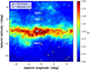 |
Fig. 1. Location of the inner Galactic bulge fields studied in this work and those from Zasowski et al. (2019; only those visible in this frame) in Galactic coordinates superimposed on the interstellar extinction map of Gonzalez et al. (2012). |
Stellar parameters of the observed stars in the northern fields of the inner Galactic bulge.
Stellar parameters of the observed stars in the southern fields of the inner Galactic bulge.
2.2. Solar neighbourhood sample
In order to minimise possible systematic uncertainties in the analysis of the abundance trends for the inner Galactic bulge, we observed similar types of stars in the Galactic discs as locally as possible. With determined abundance trends from these stars, we can search and study possible differences in a differential way. This comparison sample of 37 solar neighbourhood K giants was observed with the Immersion GRating INfrared Spectrograph (IGRINS; Yuk et al. 2010; Wang et al. 2010; Gully-Santiago et al. 2012; Moon et al. 2012; Park et al. 2014; Jeong et al. 2014) in 2016 on the 4.3 m Discovery Channel Telescope (DCT; now called the Lowell Discovery Telescope) at Lowell Observatory (Mace et al. 2018), and on the 2.7 m Harlan J. Smith Telescope at McDonald Observatory (Mace et al. 2016). The near-IR spectra provided by the IGRINS span the full H and K bands (1.45−2.5 μm) with a spectral resolving power of R ∼ 45 000. Details of observations and data reduction are explained in detail in Ryde et al. (2020), Montelius et al. (2022) and Nandakumar et al. (2022).
3. Analysis
In this study, we determined the abundance trends versus metallicity of the α-elements Mg, Si, and Ca for the inner bulge sample, as well as the local comparison sample with the same method. We made an effort to clarify the membership of the stars in our inner bulge sample by determining accurate distances and performing a dynamic analysis of the stars. In this way, we were able to disregard any star in the sample that is obviously not a bulge member. Furthermore, we adopted an updated K-band line list with determined astrophysical line strengths and improved van der Waals as well as Stark broadening parameters. We also applied and discuss non-LTE corrections for all spectral lines.
3.1. Spectroscopic analysis
3.1.1. Stellar parameters
Proper determination of the stellar parameters (i.e. Teff, log(g), [Fe/H], and ξmicro) of the stars is fundamental for an accurate and precise abundance determination. The effective temperatures used in this paper were determined in Paper I based on the relation between the effective temperature and the 12CO-band-head strength in low-resolution spectra at 2.3 μm. The method is described in Schultheis et al. (2016) and results in typical uncertainties of ±150 K. Furthermore, first estimations of the metallicities are determined using log(g) and ξmicro from Paper I. Given these metallicities, new surface gravities and microturbulences were then determined with the iterative method from Rich et al. (2017) and the empirical relation between microturbulence and surface gravity from Smith et al. (2013), respectively. Typical uncertainties in surface gravity are of ±0.3 dex after a few iterations.
The line shapes and widths are important in our analysis because we compare synthesised lines with observed ones. Therefore, we carefully analyse the widths of the lines and estimate a general macroturbulence, ξmacro, for each star using manually selected Gaussian-shaped spectral lines from Mg, Al, and Si. The updated broadening parameters for these lines will be important for the stronger lines.
The new stellar parameters are given in Tables 1 and 2. For our star sample, Teff is in the range 3400 − 4400 K and log(g) is within 0.4 − 2.0 dex. Uncertainties in the derived abundances2 are due to the fitting procedure and to the uncertainties on the stellar parameters (as shown in Rich et al. 2017; Ryde et al. 2016a) and are already well discussed in Sect. 3.4 of Paper I. It has been shown that the fitting procedure is the main contributor to the abundance error. Therefore, as in Paper I, we adopt a main abundance uncertainty of ±0.15 dex.
3.1.2. Line list
In order to determine reliable abundances for different elements from stellar spectra, we need information about the atomic physics data for the spectral lines corresponding to each element. We need the central wavelength of the line, upper and lower excitation energies of transition levels, line strengths (log gf), broadening parameters, and so on. The line list has all this information, which is necessary in order to synthesise spectral lines. VALD (Ryabchikova et al. 2015) assimilates this information from a large collection of sources, which we use as our base line list in this work.
However, we update the line list primarily with log gf values for our lines of interest (without reliable experimental log gf values), which we determined astrophysically using the high-resolution IR solar flux spectrum of Wallace & Livingston (2003). We do this by finding the value of log gf for which the respective line in the solar-flux spectrum is best fitted by the synthetic spectrum.
The collisional broadening due to neutral hydrogen, and in some cases charged particles, is important for strong lines with damping wings. For collisional broadening due to hydrogen, where possible, we have used parameters from the ABO theory (Anstee & O’Mara 1991; Anstee & O’Mara 1995; Barklem & O’Mara 1997; Barklem et al. 1998) taken from the spectral synthesis code BSYN based on routines from MARCS (Gustafsson et al. 2008). For the Mg I lines at 21 059.75 Å and the multiplet at 21 060.71−21 061.095 Å, the parameters used in Paper I for collisional broadening due to hydrogen were σ(v = 104 m s−1)=2927  , with velocity parameter α = 1.3133. These values were calculated using the impulse approximation (Kaulakys 1985, 1991; Hoang Binh & van Regemorter 1995; Osorio et al. 2015) based on Coulomb wave functions in momentum space (Hoang Binh & van Regemorter 1997; Barklem 2015), but neglecting elastic contributions because of the problem of estimating the interference between the lower and upper level contributions. In this work, rather than neglecting the elastic contribution, we estimated the maximum and minimum possible contributions, that is, the completely constructive and destructive interference cases, respectively. The mean of these two extreme elastic contributions was then added to the inelastic contribution, and we obtained σ(v = 104 m s−1)≈4440
  and α = 1.10. The error in the cross section due to the uncertainty in the elastic contribution is roughly 15%, with the overall uncertainty from this method probably being at least of order 30%.
Further, for the 21059 Å line, data for Stark broadening were extracted from the Stark-B database (Sahal-Bréchot et al. 2015), the data originating from Dimitrijevic & Sahal-Bréchot (1996). Combining the data for broadening due to electrons (e) and protons (p) with the assumption Np = Ne, and converting to the format conventionally used in many spectrum-synthesis codes for quadratic Stark broadening, we find that logΓ/Ne = −2.56 at T = 10 000 K, where Γ is the full-width at half maximum in rad s−1 and Ne is in cm−3. We find no data for the 21060.71−21061.095 Å multiplet. As this multiplet is analogous to the 21059 Å transition but in the triplet term system, we assume the Stark broadening for this multiplet to be the same as the line in the singlet system. The combination of the increased collisional broadening due to hydrogen and the strong Stark broadening significantly improved the agreement with the observed spectrum in the Sun.
In addition to the Sun spectrum, we used the high-resolution (R ∼ 100 000) IR spectrum of the well-studied Arcturus from the Arcturus atlas (Hinkle et al. 1995) to validate the updated line strengths of Fe, Mg, Si, and Ca lines. Arcturus is a well-studied reference star with reliable stellar parameters determined using various methods and is a cool giant similar to the stars investigated in this work. We determined mean values of −0.5, 0.22, 0.27, and 0.29 dex for [Fe/H] (excluding four Fe lines that were noisy or telluric affected in the Arcturus spectrum), [Mg/Fe], [Si/Fe], and [Ca/Fe], respectively, with less than 0.05 dex line-by-line dispersion for each element assuming the stellar parameters from Ramírez & Allende Prieto (2011). In addition, we used the same line list to determine the elemental abundances of the 37 solar neighbourhood giants using the same set of lines (see Sect. 3.1.4).
The central wavelengths, updated loggf values, and broadening parameters for the spectral lines used in this work are listed in Table 3. For the molecular lines, we used the line data for CO from Li et al. (2015), for CN from Sneden et al. (2014), and for OH from Brooke et al. (2016).
Spectral line data for the lines used in the present study.
3.1.3. Spectral synthesis
We used Spectroscopy Made Easy (SME version 583, Valenti & Piskunov 1996; Piskunov & Valenti 2017) for our spectral analysis. For a given set of stellar parameters, in order to generate synthetic spectra, SME interpolates a model atmosphere from a grid of spherically symmetric MARCS models computed using LTE. To account for non-LTE effects, SME applies departure coefficients by interpolating in grids. In this study, we used this type of non-LTE grid for which the departure coefficients were computed using the MPI-parallelised non-LTE radiative transfer code Balder. This code is based on the code Multi3D (Leenaarts & Carlsson 2009), which calculates the level populations for model atoms based on model atmospheres, forcing a statistical equilibrium for all levels in the ambient radiation field. For a further description of the general approach to the calculations, see Amarsi et al. (2020). Specifically, in our analysis we used the grids for Si, Mg, and Ca from Amarsi et al. (2020) and for Fe from Lind et al. (2017) and Amarsi et al. (2016; with subsequent updates in Amarsi, priv. comm.).
Moreover, SME needs the user to select spectral intervals within which the studied spectral lines lie and a line list containing the atomic and molecular data for these segments (see more about our line list in Sect. 3.1.2). Regions free from spectral lines and other features are marked manually as continuum masks allowing a local linear continuum normalisation within the interval. In the same way, the line of interest has to be marked with a line mask. Therefore, for measuring the abundance or other parameters, SME generates synthetic spectra and compares them with the observed spectrum using a χ2-minimisation in the region within the line masks.
As explained in Sect. 3.1.1, for the abundance analysis, firstly we determined the metallicity [Fe/H] using the iterative method from Rich et al. (2017). For each chemical element studied, namely iron, silicon, magnesium, and calcium, we chose a set of good-quality spectral lines (the ones used in our study are shown in Fig. 2 and listed in Table 3). Among these, we meticulously selected the best available lines for each star. To this end, each line and spectral interval were examined by eye so as to evaluate S/N and to detect disturbing artefacts or cosmic hits. In addition, line blending and fitting quality were appraised. In order to determine the final abundance value, the mean of the abundances derived from the selected lines is computed. This process permits us to obtain a precise estimate of the chemical abundances of our stars.
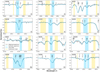 |
Fig. 2. Typical spectral fits for Si (the nine upper plots), Mg (lower left), and Ca lines (lower middle and right) used in the analysis. The stellar name is given in the upper left corner of every subplot. The black observed data are fitted with the blue synthetic spectrum. The lines of interest are marked with the blue line masks. The yellow masks show the regions in the spectrum that are used to normalise the local continuum around the lines. In some of the plots, these continuum regions are outside of the figure. The linear local continuum is always fitted with at least three continuum windows in every segment close to the line of interest. |
Given that metallicity is essential in the determination of stellar models and then in the estimation of the chemical fingerprints of stars, the iron abundances were directly determined with non-LTE corrections, contrary to the three other chemical elements for which LTE and non-LTE cases were explored and compared.
In the case of magnesium, we used the line at 21059.757 Å and the multiplet lines at 21060.710−21060.896 Å. As shown in Fig. 2, these lines are wide and very well defined and are therefore good candidates for the abundance determination as we have precise broadening values. Moreover, due to the proximity of these spectral features, we fitted all these lines simultaneously using one line mask.
Compared to the other elements of this study, there are only a few Ca lines available and these all lie on the edge of one of the detector chips. We were therefore only able to obtain Ca abundance estimates for 42 stars of our sample. Because of their proximity to CN lines, and in order to fit our selected Ca lines correctly, we fitted the nitrogen abundance via these molecular lines. Our aim is not to have an accurate estimation of nitrogen (which is a difficult chemical element to study because of its complicated molecular equilibrium with carbon and oxygen) but only to correctly fit the CN lines. Two additional Ca lines, located at 20 956.394 Å and 20 962.570 Å, are heavily blended with CN lines, and are therefore insensitive to the Ca abundance. As a consequence, we discarded them from the study.
We ensured that all the spectral lines used were not blended with any other line of our line list. Even if no suspicious line has been retained, it should be noted that there is always a risk that unknown blends or lines with unknown line strengths are not accounted for, especially for metal-rich and cool stars.
We chose a final sample, which we refer to as the Golden Sample (see Sect. 4.4), based on a sufficiently high S/N (> 40) and low line-by-line discrepancy (σlines < 0.3 dex).
3.1.4. Solar neighbourhood
The 37 solar neighbourhood stars used for comparison in this work are a subset of the Giants In the Local Disk (GILD) stellar catalogue (Jönsson et al., in prep.; which builds upon and improves the analysis described in Jönsson et al. 2017). We estimated the fundamental stellar parameters, effective temperature (Teff), surface gravity (log(g)), metallicity ([Fe/H]), and microturbulence (ξmicro) from carefully analysed optical spectra. We benchmarked these parameters against independently determined effective temperatures, Teff, from angular diameter measurements and surface gravities, log(g), from asteroseismological measurements (see Jönsson et al. 2017, for more details) with uncertainties of ±50 K for Teff, ±0.15 dex for log(g), ±0.05 dex for [Fe/H], and ±0.1 km s−1 for ξmicro. Stellar parameters of these 37 stars are in the range of 4000−5100 K in Teff, 1−3.5 dex in log(g) and −1−0.3 dex in [Fe/H]. Therefore, even though there is an overlap in Teff, the solar neighbourhood sample is strictly above 4000 K. There may therefore exist unknown systematic uncertainties in Teff, which should be kept in mind while comparing the two samples. This is an improvement that could be made in the future when such observations exist.
With accurate stellar parameters known, we carried out a detailed analysis of the same set of Si, Mg, and Ca lines used for the bulge stars in order to determine their respective abundances. In addition, we use the same set of stellar atmosphere grids, the same version of the SME, the same non-LTE corrections, and the same line list as we use for the bulge stars. We therefore carried out a consistent spectroscopic analysis of the bulge and solar neighbourhood giant stars to determine their elemental abundances. Needless to say, one obvious difference between the IGRINS spectra of the bright nearby solar neighbourhood stars and the CRIRES spectra of the faint and distant bulge stars is the better S/N, which naturally affects the precision of the abundance estimates.
3.2. Dynamical analysis
While our sample size is relatively modest, we undertook a basic dynamical analysis in order to ensure membership of the inner Galactic bulge. Therefore, astrometric parameters are necessary as initial conditions to study dynamics. Among the 72 stars, 63 were cross-matched with Gaia EDR3 (Gaia Collaboration 2016, 2021) in order to obtain their proper motions. To ensure reliable values, a proper motion error limit is set at 0.3 mas yr−1. In addition, updated distances were determined (see Sect. 4.2) and radial velocities were measured using the strong and clear Mg lines.
We used the software package AGAMA (Vasiliev 2019) to compute the orbits of our stars up to 10 Gyr. As we are studying inner bulge stars, we used a combination of three gravitational potentials: a disc, a halo, and a bulge/bar. More precisely, we used the disk and halo components of the MWPotential2014 (Bovy 2015) and the bar potential from Launhardt et al. (2002). A typical (clock-wise) rotation pattern speed about Ωb = 40 km s−1 kpc−1 was taken into account for the bar (Portail et al. 2017) which is at an angle of α = 25° from the line of sight towards the Galactic centre. We use these orbital parameters to assign the bulge membership in addition to the calculated distances (see Sect. 4.3).
4. Results
We now discuss our new abundance measurements of α elements for giants in the inner Galactic bulge. Moreover, we discuss the re-determined distances of the stars and therefore their bulge-membership.
4.1. Abundances
Figure 3 shows typical fits of a Si line, Ca line, and the Mg lines. The sensitivity of the abundance determination is shown by varying the abundance by ±0.15 dex (the choice of this uncertainty value is explained Sect. 3.1.1) plotted as a band around the observed spectrum.
 |
Fig. 3. Typical spectral fits for Si, Mg, and Ca lines with a variation band of ±0.15 dex in abundance. The upper panel shows fitted lines for stars with a good S/N whereas the lower panel shows those for stars with a poor S/N. |
4.1.1. LTE and non-LTE comparison
In order to investigate the effects of non-LTE corrections and to be able to compare our results with those from Paper I, in which only the LTE case was explored, we determined Si, Mg, and Ca abundances calculated both with LTE and non-LTE level populations, affecting both the source function and the line opacity. Therefore, LTE and non-LTE abundance trends for [Si/Fe], [Mg/Fe], and [Ca/Fe] are shown Fig. 4 with the LTE results from Paper I superimposed (except for Ca which was not measured in Paper I). In addition, the running mean of each trend was computed and is plotted in Fig. 4.
 |
Fig. 4. Comparison of our [Si/Fe], [Mg/Fe], and [Ca/Fe] versus [Fe/H] trends in LTE and non-LTE. The comparison sample for Si and Mg is from Nandakumar et al. (2018) and is shown in grey. The upper row shows our trends in red while assuming LTE in the line formation. The middle row shows our trends in blue when assuming non-LTE instead. The lower row shows the running mean of our trends with and without LTE in order to demonstrate the differences more clearly. |
A few differences between LTE and non-LTE can be seen. For [Si/Fe], the non-LTE trend is indeed slightly stronger and by looking at its running mean, we see that this trend is only slightly lower than the LTE one. For [Mg/Fe], the difference is clearly noticeable; the non-LTE trend is much stronger, showing less scatter, especially for higher metallicities. Moreover, there is a significant offset of ∼0.1−0.15 dex between the two trends. Finally, for [Ca/Fe] there is almost no difference between the two cases, and only a very slight offset is visible. This latter fact is further discussed in Sect. 5.2.
By comparing the line-by-line discrepancy values for LTE and non-LTE cases, we see that they are lower in the latter case, which justifies our choice to take into account non-LTE effects, as this appears to improve the accuracy of our spectral analysis. Moreover, we note that using non-LTE decreases the scatter in the [α/Fe] versus [Fe/H] trends. From now on, we therefore focus on the non-LTE abundances.
4.1.2. Silicon and magnesium
In Fig. 4 we show our new [Si/Fe] and [Mg/Fe] trends as function of metallicity compared to the ones derived in Paper I. The uncertainties are the same for the old and the new abundances: 0.15 dex. Besides the fact that our [Si/Fe] and [Mg/Fe] trends follow a typical α-element trend, we observe that there is no plateau at supersolar metallicities for either silicon or magnesium; our trends keep going down. Also, our Si abundances are slightly higher (+0.14 dex in average) and our Mg abundances slightly lower (−0.14 dex in average) than the results from Paper I. Compared to the latter, where [Si/Fe] results were showing a lower dispersion than [Mg/Fe], we get the opposite in our study. This is explained by the fact that the Mg lines used are more sensitive to non-LTE effects than the Si lines (see Fig. 4).
4.1.3. Calcium
The determination of calcium abundances for our inner bulge stars is new compared to Paper I and is therefore one of the major novelties of this study. As mentioned in Sect. 3.1.3, only the few stars with satisfactory Ca lines have a calcium abundance estimation (see final values in Table 2). We can see that our Ca trend is more dispersed (which could be simply due to the lack of stars) and higher values are seen for metal-rich stars, which is different from our Si and Mg trends.
4.2. Distances
We determined the spectro-photometric distances using the stellar parameters Teff, log(g), and [Fe/H] (Rojas-Arriagada et al. 2014; Schultheis et al. 2017) together with the near-IR photometry J, H, and K and associated errors, in order to simultaneously compute the most likely line-of-sight distance and reddening by isochrone fitting using PARSEC isochrones. Here we use the same method as that described in Rojas-Arriagada et al. (2017), where we consider a set of isochrones spanning ages from 1 to 13 Gyr in steps of 1 Gyr and metallicities from −2.2 to +0.5 dex in steps of 0.1 dex. As in Rojas-Arriagada et al. (2017), besides computing the distance from the observed stars to the whole set of model stars, we calculate weights for each star, which depend on: the evolutionary speed of the model stars; the fact that the number of stars per mass is not uniform, which is given by the IMF; and an exponential weight associated with the distance of the observed stars with respect to the model. The typical uncertainties are on the order of 20%−40% but we find no systematic differences in comparison to distances obtained by a Bayesian approach for example (e.g. Santiago et al. 2016). The obtained distances permit us to analyse the bulge membership of our sample; see Sect. 4.3. We note that we do not calculate the distances of the Galactic centre field because we lack the J magnitudes. From the heliocentric distances, we computed the galactocentric radial distance 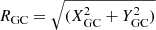 where XGC and YGC are the cartesian coordinates.
4.3. Bulge membership
Figure 5 displays the distribution of the galactocentric distances (RGC) where we see a peak in the distribution at RGC ∼ 1.5 kpc. We also indicate the typical intrinsic depth of the bulge with RGC ≤ 3.5 kpc (see e.g. Rojas-Arriagada et al. 2017, 2020; Zasowski et al. 2019). Four stars (bp3-06, bp2-06, bm1-13, bm1-17) show larger distances going up to RGC ∼ 12.0 kpc, indicating that those do not belong to the inner bulge. They all have low metallicities ([Fe/H] ∼ −1.0) and are enhanced in the α-elements and could therefore belong either to the thick disc or to the halo population. Thus, compared to Paper I where no star was found outside of the bulge, in this study we exclude those four stars from further analysis, resulting in a total sample of 59 stars with determined distances.
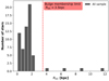 |
Fig. 5. Histogram of the galactocentric radial distances (computed in Sect. 4.2) of the stars in our sample for which values are available. The typical intrinsic depth of the bulge is indicated by the red dashed line. |
All the stars of our sample were spectrally analysed using the method explained in Sect. 3.1.3, except the star bp2-06. Indeed, due to the very low metallicity of this latter object (the estimation for bp2-06 from Paper I gives −1.8 dex), none of our Fe lines are usable for determining it directly. However, thanks to our dynamical analysis introduced in Sect. 3.2 and to our broad Mg lines, we can estimate its metallicity. As explained in Sect. 4.2 and shown in Table 8, the galactocentric radial distance of bp2-06 is about 8.7 kpc (using its metallicity estimation from Paper I), which demonstrates that it does not belong to the inner bulge. In addition, its simulated orbit shown in Fig. 6 supports the latter finding and provides further information about its movements in the Galaxy.
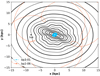 |
Fig. 6. Comparison of the orbits in the Cartesian galactocentric (x, y) plane of bp3-01 found in the bulge and bp2-06 found outside of the bulge. The black contours show the surface density of the stellar component of our combination of gravitational potentials. |
These results lead us to conclude that bp2-06 may be a halo star and therefore it ought to have a typical Mg abundance for a halo star of about ∼0.4 dex (see e.g. Edvardsson et al. 1993). A magnesium-based metallicity can therefore be estimated by selecting a range of iron abundances [Fe/H] and corresponding log(g) and ξmicro and by fitting our Mg spectral feature for each of these sets of values. We finally obtain a metallicity of about −2.03 dex, which allows us to obtain a Mg abundance of about 0.4 dex for this star. Such a low metallicity, together with its orbits, leads us to reject the notion that this star is in the inner bulge. It is therefore excluded from our inner bulge sample.
We also checked the derived orbital parameters for our bulge stars sample, such as apocentric radius (Rapo) and maximum vertical height (zmax). Except for the four stars with larger distances mentioned above (bp3-06, bp2-06, bm1-13, bm1-17), our sample shows typical orbital parameters for the bulge, with the majority of stars lying within Rapo < 3 kpc and zmax < 1.5 kpc and with high eccentricities. We do not find any trends in the orbital parameters with metallicity and/or abundances, but a larger sample is clearly needed in order to obtain statistically significant results.
4.4. The Golden Sample
The objective of this work is to derive the most precise abundance trends as possible for the inner Galactic bulge. In this context, we construct a clean sample, referred to as the Golden Sample, which contains stars belonging to the inner bulge as determined in Sect. 4.2 and that have sufficiently high-quality spectra. To select these stars (i) we require a minimum S/N of 40 (see Sect. 3.1.3) and (ii) as explained in Sect. 4.3, we exclude stars with RGC > 3.5 kpc.
Therefore, because of an insufficient S/N, we discarded the stars bp2-02, bp1-01, GC1, GC20, GC25, GC27, GC28, GC37, bm1-06, bm1-18, and bm1-19 from the abundance analysis. It should be noted that the latter are mainly from the Galactic centre field, which is expected as it corresponds to the innermost region studied here. Similarly, the stars bp3-06, bp2-06, bm1-13, and bm1-17 are excluded because of their excessive distances. From the original sample of 72 stars, our Golden Sample is therefore reduced to 57 stars. The latter are highlighted in bold face in Tables 1, 2, 4–9.
Si abundances of the observed stars in the northern fields.
Si abundances of the observed stars in the southern fields.
Mg and Ca abundances of the observed stars in the northern fields.
Mg and Ca abundances of the observed stars in the southern fields.
Distances of the observed stars in the northern fields.
Distances of the observed stars in the southern fields.
Moreover, we computed the line-by-line discrepancy, σlines (given in Tables 4–7), for every star abundance, which is the standard deviation of the used line abundance values. Therefore, in addition to the selection made for the construction of our Golden Sample, we require σlines < 0.3 for each chemical element. As explained in Sect. 3.1.3, due to the fact that we used only one spectral feature for magnesium, the line-by-line discrepancy is zero for this element. This selection criterion is therefore useful to our analysis, but as its value strongly depends on the number of used lines, caution must be taken when using it; for example, abundances determined with only one line cannot be evaluated by this criterion.
5. Discussion
Here, we discuss our results presented in Sect. 4 and compare them to a local sample of solar neighbourhood stars, for which we used the same lines and spectral analysis method (we refer the reader to Sects. 2.2 and 3.1.4 for more details). Moreover, our abundance trends are also compared to the APOGEE inner bulge sample from Zasowski et al. (2019; hereafter referred to as the APOGEE sample). The APOGEE sample has been updated with the latest APOGEE DR17 release (Abdurro’uf et al. 2022) covering about 4000 stars with RGC < 4 kpc. Finally, we discuss our abundances in context of a tailored chemical-evolution model for the inner bulge.
5.1. Silicon and magnesium
The NLTE Si and Mg abundance trends for our Golden Sample of the inner bulge are shown in Fig. 7. These are compared to our local star sample in the upper panel of the figure. This comparison provides a more direct test to look for differences or similarities between the populations, as the analyses of the stars are designed to be as similar as possible, thereby minimising any systematic uncertainties. As indicated in Sect. 3.1.4, even if the local sample has been selected in the most reasonable way possible, the potential existence of unknown systematic uncertainties in Teff should be kept in mind while comparing the two samples. However, a larger scatter is expected for the inner bulge sample, due to the most obvious and only significant difference between the analyses, which is the S/Ns. In general, we see that the Si and Mg trends for the inner bulge and local thin and thick discs are in very good agreement.
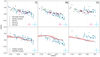 |
Fig. 7. NLTE [Si/Fe], [Mg/Fe], and [Ca/Fe] vs. [Fe/H] trends of our Golden Sample of the inner bulge shown in light blue and compared to solar neighbourhood stars in purple (thin disc), green (thick disc), and dark blue (halo) in the upper panel and compared to the running mean of the updated APOGEE DR17 sample from Zasowski et al. (2019) plotted in red in the lower panel. |
However, our inner bulge stars extend to higher metallicities. Furthermore, although based on few stars, the local sample shows a tendency to ‘flatten off’ at [Fe/H] > 0.25 dex. The inner bulge sample, on the other hand, clearly shows a continuous downward trend with increasing metallicity (Johnson et al. 2013 report a similar result for several α elements in outer bulge fields; moreover, chemical-evolution models suggest this is indeed to be expected; see Sect. 5.3), albeit with a significant scatter in the abundance ratios. This is true for both the [Si/Fe] and [Mg/Fe] trends. Our derived Mg abundances show the steepest slope of decreasing Mg with increasing [Fe/H] with a mean dispersion of 0.10 dex (see Fig. 4). More stars and further investigations into the cause of the increased scatter at supersolar metallicities for the inner bulge stars are needed in order to be able to claim any difference in the slopes of the trends for the two populations.
In the lower panel of Fig. 7, the Si and Mg trends for our inner bulge stars are compared to those of the inner bulge APOGEE sample from Zasowski et al. (2019). These data result from different analysis methods and a systematic shift might therefore be expected. Silicon is the α-element with the lowest dispersion in APOGEE, which is also seen in other IR studies (Rich & Origlia 2005; Schultheis et al. 2017; Ryde et al. 2010). We see good agreement overall, within the uncertainties, except for the highest metallicities. There is, on the other hand, a significant and systematic offset between the data sets for the [Mg/Fe] trends, with the metal-rich regime showing the largest differences, namely of up to 0.4 dex. We note that Mg and Si are hailed to be the α-elements measured with the greatest precision by APOGEE (see e.g. Jönsson et al. 2018; Schultheis et al. 2017) and Mg does not show signs of any temperature dependency. As this offset is also the case for our local disc sample, and the APOGEE [Mg/Fe] trend corresponds to what is expected for a bulge/thick disc trend (see e.g. Bensby et al. 2014), we believe that our [Mg/Fe] trend is systematically too low by a few times 0.1 dex. As noted above, such a shift might be expected in light of the differences in the analysis methods, such as the choice of lines used, whether or not NLTE effects are used, and whether or not those effects are correct in magnitude. Therefore, a differential comparison of the local and the inner bulge stars is very important.
We also note that a flattening in [Si/Fe] and [Mg/Fe] trends is seen for the APOGEE sample for metal-rich stars, that is, [Fe/H] > 0.0. Santos-Peral et al. (2020) demonstrated that the normalisation procedure has an important impact on the derived abundances and that narrow normalisation windows around the studied lines improves the precision and leads to a decreasing trend in the abundance even at supersolar metallicities. This might be an explanation for the differences. However, we note that this explanation would not explain this levelling-off tendency for our local sample.
The APOGEE sample suffers from some slight temperature dependencies of Si abundance, which is not the case for our Golden Sample, as shown in Fig. 8 (only an expected trend is visible: the warmer stars are more metal poor). This might affect the more metal-rich APOGEE stars, as these tend to be cooler. However, the [Si/Fe] difference in the slope at supersolar metallicities is less obvious when comparing with our inner bulge sample, up to [Fe/H] ∼ 0.3. As shown in Fig. 4, NLTE corrections for Si are also very small, and so this should not cause any differences.
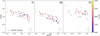 |
Fig. 8. NLTE [Si/Fe], [Mg/Fe], and [Ca/Fe] vs. [Fe/H] trends of our Golden Sample of the inner bulge colour coded with Teff showing no bias with temperature. |
5.2. Calcium
The Ca abundances determined for the local solar neighbourhood sample show only slightly larger scatter compared to the local [Si/Fe] and the [Mg/Fe] trends. However, the [Ca/Fe] trend for our golden sample of the inner bulge shows the largest intrinsic dispersion compared to Mg and Si. This is in part due to problems with the Ca lines, such as the fact that they are situated close to the edge of the detector in the CRIRES setup. This is not the case for the solar neighbourhood sample, which is observed with the IGRINS spectrometer, covering the full K band with no gaps. Nevertheless, we see a general agreement in [Ca/Fe] between the solar neighbourhood and the Golden Sample.
A clear offset compared with the APOGEE sample can be seen. Schultheis et al. (2017) noted that, for Baade’s window, the Ca abundances of APOGEE are systematically ∼0.15 dex lower than those reported by Rich & Origlia (2005), Fulbright et al. (2007), and Gonzalez et al. (2011). The APOGEE trend is also lower compared to what is expected for the bulge/thick disc trend (see e.g. Bensby et al. 2014). This shift would put our local sample and APOGEE’s trend in closer agreement. The NLTE corrections for Ca could also be underestimated for the K band lines, leading to overly high Ca abundances with respect to APOGEE. However, the Ca NLTE corrections (Amarsi et al. 2020) for the H band are small and the solar disc trends with these NLTE corrections show good agreement with the [Ca/Fe] trends for the disc determined from optical lines (Montelius et al. 2022). There is therefore no direct reason to believe that these corrections should be underestimated. As for the other α-elements, here we again see the flattening in APOGEE for the high-metallicity stars.
5.3. A new chemical-evolution model of the inner Galactic bulge
In this section, we present a new chemical-evolution model designed to reproduce the NLTE abundance ratios and metallicity distribution function (MDF) of the inner bulge stars. First, in Sect. 5.3.1, we compare the new NLTE data for the inner bulge with the chemical-evolution model of Matteucci et al. (2019) based on the one-infall scenario designed for the Galactic bulge. Subsequently, in Sect. 5.3.2, we compare the data to a two-infall model. While such simple approaches to galaxy evolution cannot account for the full complexity of galaxy formation, they have served as useful reference models in the literature for studying the impact of single or multiple episodes of galactic star formation on the chemical signatures in stellar populations.
5.3.1. Testing the one-infall chemical-evolution model
In the left panel of Fig. 9, we compare the NLTE [Mg/Fe] versus [Fe/H] data presented in Sect. 4.1.2 with the one-infall chemical-evolution model for the Galactic bulge of Matteucci et al. (2019). In this model, the bulge follows a fast gravitational collapse scenario (Larson 1976) and is supposed to form by accretion of a single fast gas-infall event on a timescale of τ = 0.1 Gyr. The proposed model was capable of reproducing Gaia-ESO bulge stars of Rojas-Arriagada et al. (2017) adopting the Salpeter (1955) IMF. However, we note from Fig. 9 that the NLTE data presented in this study are not reproduced by the model. A better agreement is obtained with the Kroupa et al. (1993) IMF. As highlighted in the VINTERGATAN simulation (Agertz et al. 2021), the scatter in the data with high-[α/Fe] abundance ratio values across the entire galaxy is largely set by the gas-consumption timescales in star forming clouds (see Fig. 9 in Renaud et al. 2021b). Gas with short depletion times shows the highest values of [α/Fe] at fixed [Fe/H] values. This is due to supernova-enriched gas being trapped more easily in dense clouds where the depletion time is short. It is worth noticing that in the VINTERGATAN simulation, the scatter in the high-alpha sequence is present in both the in situ formed stars and the accreted stars (see Fig. 8 in Renaud et al. 2021b).
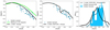 |
Fig. 9. One-infall chemical-evolution model predictions for the Galactic bulge. Left panel: effects of different IMF on the one-infall chemical-evolution model. With the green line, we show the model presented in Matteucci et al. (2019) assuming the Salpeter (1955) IMF, whereas with the black line we show the same model but with the Kroupa et al. (1993) IMF. Blue dots are the [Mg/Fe] abundances for our Golden Sample. Middle panel: [Mg/Fe] vs. [Fe/H] for the one-infall model with the Kroupa et al. (1993) IMF, where a 250 Myr pause in star formation has been applied. Right panel: Kernel density estimation of the MDF of the same model as in the middle panel (black line) compared with the histogram and KDE of the NLTE stars distribution (blue histogram and line). |
In the middle panel, following Matteucci et al. (2019), in order to reproduce the bimodality in both in the [Mg/Fe] versus [Fe/H] space and in the MDF, we try a 250 Myr pause in star formation. The chemical-evolution model characterised by a unique gas-accretion event coupled with a pause in star formation is able to predict the gap in the [X/Fe] versus [Fe/H] observed in APOGEE bulge data (middle panel), but completely fails to properly reproduce the two stellar populations in the MDF (see right panel).
5.3.2. Inner-bulge stellar populations with the two-infall model
In the previous section, we show that the classical one-infall chemical-evolution model does not seem to be the correct scenario to properly reproduce the chemical properties of the inner bulge.
Here, we consider the possibility that two gas-accretion events are responsible for the chemical signatures impressed in the NLTE abundance ratios. The presence of two distinct sequences in the chemical abundances in the Galactic bulge was pointed out by Matteucci et al. (2019) and Queiroz et al. (2020) based on analyses of APOGEE stars. In particular, in Queiroz et al. (2020), the Galactic disc dichotomy in the abundance ratios [α/Fe] versus [Fe/H] seemed to extend up to the innermost regions of the disc up to the bulge. The complex nature of the Galactic bulge structures has already been addressed by theoretical models with the introduction of two different stellar populations. Samland & Gerhard (2003), by means of a dynamical model, predicted the existence of two bulge populations: one originating from an early collapse and the other formed late in the bar through secular evolution (e.g. Combes et al. 1990; Norman et al. 1996; Kormendy & Kennicutt 2004; Athanassoula 2005). These results suggest the two-infall chemical-evolution model may represent the scenario capable of reproducing the chemical evolution that we find in the Golden Sample.
In the context of the two-infall model, the adopted analytical expression for the gas infall rate is:
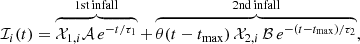 (1)
(1)
where τ1 = 0.4 Gyr and τ2 = 2 Gyr are the timescales of the two distinct gas-infall episodes. The Heaviside step function is represented by θ. 𝒳1, i and 𝒳2, i are the abundance by mass unit of the element i in the infalling gas for the first and second gas infall, respectively. The quantity tmax is the time of the maximum infall rate on the second accretion episode; that is, it indicates the delay between the two peaks of infall rates. In this model, gas outflow occurs during the first infall phase – in which the accretion of gas happens on a short timescale, and is therefore faster – with a rate proportional to the SFR through a free parameter. The outflow rate is defined as
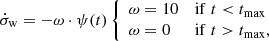 (2)
(2)
where ω is the mass loading of the wind. Values of 10 or even greater for this latter parameter are expected in galaxies with stellar masses < 109 M⊙ (e.g. Chisholm et al. 2017). Hence, the large mass-loading factors experienced by the inner bulge in a scenario of an early, fast collapse (first gas infall episode) can impose important constraints on the host environment of the stars residing in the bulge (or possibly even the mass of the MW bulge when these stars formed; see analysis for MW-mass systems by van Dokkum et al. 2013).
The star formation rate (SFR) is expressed as the Kennicutt (1998) law,
 (3)
(3)
where σg is the gas surface density and k = 1.5 is the exponent. The quantity ν is the star formation efficiency (SFE) and this has been set to the value of 10 Gyr−1, a value compatible with previous chemical-evolution models for the Galactic bulge (Matteucci et al. 2019). Following Grieco et al. (2012), we impose that for the second gas infall, a chemical enrichment must be obtained from the model of the early collapse phase, corresponding to [Fe/H] = −1 dex.
From Fig. 10, we note that our model predictions accurately reproduce the Golden Sample data (NLTE) both in the [Mg/Fe] versus [Fe/H] and [Si/Fe] versus [Fe/H] relations. It is worth mentioning that, for Mg, the agreement between data and the model substantially improves if we consider NLTE stars. Nevertheless, the proposed two-infall model underestimates the data in the [Ca/Fe] versus [Fe/H] space. This is due to the adopted nucleosynthesis prescriptions. In fact, we make use of the ones suggested by Romano et al. (2010, in their model 15), and we refer the reader to this article for details. We stress here that in Fig. 22 of this latter paper, model predictions for the Ca in the solar neighbourhood also substantially underestimate that data sample in the [Ca/Fe] versus [Fe/H] space (see also the discussion in Spitoni et al. 2023).
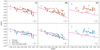 |
Fig. 10. LTE (upper panel) and NLTE (lower panel) [Si/Fe], [Mg/Fe], and [Ca/Fe] vs. [Fe/H] trends of our Golden Sample compared with the two-infall bulge chemical model constructed Sect. 5.3.2. |
The histogram and kernel density estimate (KDE) of the MDF of our Golden Sample (see Sect. 4.4 for more details about the star selection) is shown Fig. 11. In this figure, we can also appreciate that our two-infall model for the inner bulge accurately reproduces the MDF of the Golden Sample. It is important to underline that the purpose of this study is not to analyse the MDF in the inner Galactic bulge in detail, since the targeted stars have not been specifically selected using an unbiased method concerning this parameter. The stars were selected in such a way that they are sufficiently bright and therefore do not suffer from excessive interstellar reddening but cover a wide range in the colour and therefore effective temperature. Because of our limited sample size, we do not address any corrections concerning the selection function. However, MDF studies so far (see e.g. Rojas-Arriagada et al. 2020; Nandakumar et al. 2017) do not reveal strong selection effects on the shape of the MDF. Compared to Paper I, no particular offset is observed with our new metallicity values.
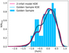 |
Fig. 11. Histogram and kernel density estimation of the metallicity distribution function of our Golden Sample stars (blue histogram and blue line) compared to those predicted by our chemical-evolution model (pink line) presented Sect. 5.3.2. |
6. Conclusions
We analysed the α-element composition of 72 M giants in the inner Galactic bulge from Nandakumar et al. (2018) using high-resolution CRIRES spectra. To this end, we determined precise silicon, magnesium, and calcium abundances using a meticulous star-by-star analysis. In addition, thanks to a recently updated K-band line list, improved broadening parameters, a more precise macro-turbulence estimation, and NLTE corrections, this paper provides one of the most detailed studies of α-abundance trends in the inner bulge carried out so far. This study can be used as a kind of benchmark for future spectroscopic surveys such as the upcoming MOONS galactic survey (Gonzalez et al. 2020).
Thanks to a membership study using distance estimations and simulated orbits, we find that four stars of our sample are not bulge members. With additional selections based on S/N and line-by-line discrepancy, we constructed a clean sample of our inner bulge stars.
We compare our α-abundance trends in LTE and NLTE cases and find the NLTE corrections reduce scatter overall, with Mg having the most reduction. However, the NLTE analysis results in ∼0.1 dex lower [Mg/Fe]; applying NLTE corrections gives a noticeably lower trend in [Mg/Fe] versus [Fe/H]. Calcium owes its higher dispersion to the lower quality of the Ca lines used. NLTE [α/Fe] versus [Fe/H] trends of our inner bulge stars and those for thin/thick discs of our solar neighbourhood sample obtained using the same lines and spectral analysis show similar behaviour, with the bulge sample extending to +0.5 dex in [Fe/H], +0.3 dex beyond the solar neighborhood sample. For both Si and Mg, the bulge trend at suprasolar metallicity is lower than the solar vicinity, especially for Mg. This is striking and is contradictory to the canonical alpha enhancement expected for bulge giants; this trend requires confirmation.
However, for metal-rich stars with [Fe/H] > 0.3, we observe a flattening in the [Si/Fe] and [Mg/Fe] thin-disc trends, which we do not find in our inner bulge trends nor in our chemical-evolution model trends. Additional solar neighbourhood stars for these values of metallicity would be needed to validate this difference.
Based on our derived MDF and α-abundance trends, we constructed a tailored chemical-evolution model for the inner Galactic bulge. This latter is highly consistent with silicon and magnesium abundances. In the case of calcium, our model underestimates the abundance values because of the nucleosynthesis prescriptions selected in this work. According to this model, two gas-accretion events with timescales of 0.4 Gyr and 2 Gyr would explain the chemical fingerprints in the α-elements of these inner-bulge stars. However, a larger sample of high-quality abundances in the inner bulge is clearly needed in order to confront them with galactic chemical-evolution models.
Here defined purely geometrically as the inner 10° of the Milky Way (Barbuy et al. 2018).
The solar value used in this study is from Grevesse et al. (2007).
Here σ is the broadening cross section and α describes the velocity dependence assuming a power law σ ∝ v−α.
Acknowledgments
We are grateful to the referee for her/his useful comments. We would like to thank the IGRINS team and especially Dr. G. Mace for excellent help and support. Further, we would like to acknowledge to enlightening discussions with Dr. A. Amarsi about NLTE calculations. This work used the Immersion Grating Infrared Spectrometer (IGRINS) that was developed under a collaboration between the University of Texas at Austin and the Korea Astronomy and Space Science Institute (KASI) with the financial support of the Mt. Cuba Astronomical Foundation, of the US National Science Foundation under grants AST-1229522 and AST-1702267, of the McDonald Observatory of the University of Texas at Austin, of the Korean GMT Project of KASI, and Gemini Observatory. The paper is based on observations collected at the European Southern Observatory, Chile, program numbers 089.B-0312(A)/VM/CRIRES, 089.B-0312(B)/VM/ISAAC, 091.B-0369(A)/VM/SOFI, and 091.B-0369(B)/SM/CRIRES. N.R. acknowledges support from the Royal Physiographic Society in Lund through the Stiftelsen Walter Gyllenbergs fond and Märta och Erik Holmbergs donation. N.R. ackowledges the support from Magnus Bergvalls stiftelse. M.S. and N.N. acknowledge the funding of the BQR Lagrange. G.N. acknowledges the support from the Wenner-Gren Foundations and the Royal Physiographic Society in Lund through the Stiftelsen Walter Gyllenbergs fond. O.A. and F.R. acknowledge financial support from the Knut and Alice Wallenberg Foundation and the Swedish Research Council (grant 2019-04659). E.S. received funding from the European Union’s Horizon 2020 research and innovation program under SPACE-H2020 grant agreement number 101004214 (EXPLORE project). P.S.B. acknowledges support from the Swedish Research Council through an individual project grant with contract No. 2020-03404. N.N. thanks Gabriele Contursi for helpful comments on figures.
References
- Abdurro’uf, Accetta, K., Aerts, C., et al. 2022, ApJS, 259, 35 [NASA ADS] [CrossRef] [Google Scholar]
- Agertz, O., Renaud, F., Feltzing, S., et al. 2021, MNRAS, 503, 5826 [NASA ADS] [CrossRef] [Google Scholar]
- Amarsi, A. M., Lind, K., Asplund, M., Barklem, P. S., & Collet, R. 2016, MNRAS, 463, 1518 [NASA ADS] [CrossRef] [Google Scholar]
- Amarsi, A. M., Lind, K., Osorio, Y., et al. 2020, A&A, 642, A62 [EDP Sciences] [Google Scholar]
- Anstee, S. D., & O’Mara, B. J. 1991, MNRAS, 253, 549 [NASA ADS] [CrossRef] [Google Scholar]
- Anstee, S. D., & O’Mara, B. J. 1995, MNRAS, 276, 859 [Google Scholar]
- Athanassoula, E. 2005, MNRAS, 358, 1477 [NASA ADS] [CrossRef] [Google Scholar]
- Barbuy, B., Chiappini, C., & Gerhard, O. 2018, ARA&A, 56, 223 [Google Scholar]
- Barklem, P. S. 2015, https://doi.org/10.5281/zenodo.50218 [Google Scholar]
- Barklem, P. S., & O’Mara, B. J. 1997, MNRAS, 290, 102 [Google Scholar]
- Barklem, P. S., O’Mara, B. J., & Ross, J. E. 1998, MNRAS, 296, 1057 [Google Scholar]
- Bensby, T., Feltzing, S., & Oey, M. S. 2014, A&A, 562, A71 [NASA ADS] [CrossRef] [EDP Sciences] [Google Scholar]
- Bovy, J. 2015, ApJS, 216, 29 [NASA ADS] [CrossRef] [Google Scholar]
- Brault, J., & Noyes, R. 1983, ApJ, 269, L61 [Google Scholar]
- Brooke, J. S. A., Bernath, P. F., Western, C. M., et al. 2016, J. Quant. Spectr. Rad. Transf., 168, 142 [NASA ADS] [CrossRef] [Google Scholar]
- Buder, S., Sharma, S., Kos, J., et al. 2021, MNRAS, 506, 150 [NASA ADS] [CrossRef] [Google Scholar]
- Chisholm, J., Tremonti, C. A., Leitherer, C., & Chen, Y. 2017, MNRAS, 469, 4831 [NASA ADS] [CrossRef] [Google Scholar]
- Civiš, S., Ferus, M., Chernov, V. E., & Zanozina, E. M. 2013, A&A, 554, A24 [NASA ADS] [CrossRef] [EDP Sciences] [Google Scholar]
- Combes, F., Debbasch, F., Friedli, D., & Pfenniger, D. 1990, A&A, 233, 82 [NASA ADS] [Google Scholar]
- Dimitrijevic, M. S., & Sahal-Bréchot, S. 1996, A&AS, 117, 127 [NASA ADS] [CrossRef] [EDP Sciences] [Google Scholar]
- Edvardsson, B., Andersen, J., Gustafsson, B., et al. 1993, A&A, 275, 101 [NASA ADS] [Google Scholar]
- Fulbright, J. P., McWilliam, A., & Rich, R. M. 2007, ApJ, 661, 1152 [NASA ADS] [CrossRef] [Google Scholar]
- Gaia Collaboration (Prusti, T., et al.) 2016, A&A, 595, A1 [NASA ADS] [CrossRef] [EDP Sciences] [Google Scholar]
- Gaia Collaboration (Brown, A. G. A., et al.) 2021, A&A, 650, C3 [EDP Sciences] [Google Scholar]
- Gonzalez, O. A., Rejkuba, M., Zoccali, M., et al. 2011, A&A, 530, A54 [NASA ADS] [CrossRef] [EDP Sciences] [Google Scholar]
- Gonzalez, O. A., Rejkuba, M., Zoccali, M., et al. 2012, A&A, 543, A13 [NASA ADS] [CrossRef] [EDP Sciences] [Google Scholar]
- Gonzalez, O. A., Mucciarelli, A., Origlia, L., et al. 2020, The Messenger, 180, 18 [NASA ADS] [Google Scholar]
- Grevesse, N., Asplund, M., & Sauval, A. J. 2007, Space Sci. Rev., 130, 105 [Google Scholar]
- Grieco, V., Matteucci, F., Pipino, A., & Cescutti, G. 2012, A&A, 548, A60 [NASA ADS] [CrossRef] [EDP Sciences] [Google Scholar]
- Gully-Santiago, M., Wang, W., Deen, C., & Jaffe, D. 2012, SPIE Conf. Ser., 8450, 84502S [NASA ADS] [Google Scholar]
- Gustafsson, B., Edvardsson, B., Eriksson, K., et al. 2008, A&A, 486, 951 [NASA ADS] [CrossRef] [EDP Sciences] [Google Scholar]
- Hinkle, K., Wallace, L., & Livingston, W. 1995, PASP, 107, 1042 [Google Scholar]
- Hoang Binh, D., & van Regemorter, H. 1995, J. Phys. B: At. Mol. Opt. Phys., 28, 3147 [NASA ADS] [CrossRef] [Google Scholar]
- Hoang Binh, D., & van Regemorter, H. 1997, J. Phys. B: At. Mol. Opt. Phys., 30, 2403 [NASA ADS] [CrossRef] [Google Scholar]
- Jeong, U., Chun, M. Y., Oh, J. S., et al. 2014, SPIE Conf. Ser., 9154, 91541X [NASA ADS] [Google Scholar]
- Johnson, C. I., Rich, R. M., Kobayashi, C., et al. 2013, ApJ, 765, 157 [Google Scholar]
- Johnson, C. I., Rich, R. M., Kobayashi, C., Kunder, A., & Koch, A. 2014, AJ, 148, 67 [Google Scholar]
- Johnson, C. I., Rich, R. M., Young, M. D., et al. 2020, MNRAS, 499, 2357 [NASA ADS] [CrossRef] [Google Scholar]
- Johnson, C. I., Rich, R. M., Simion, I. T., et al. 2022, MNRAS, 515, 1469 [NASA ADS] [CrossRef] [Google Scholar]
- Jönsson, H., Ryde, N., Nordlander, T., et al. 2017, A&A, 598, A100 [NASA ADS] [CrossRef] [EDP Sciences] [Google Scholar]
- Jönsson, H., Allende Prieto, C., Holtzman, J. A., et al. 2018, AJ, 156, 126 [Google Scholar]
- Kaeufl, H. U., Ballester, P., Biereichel, P., et al. 2004, SPIE Conf. Ser., 5492, 1218 [NASA ADS] [Google Scholar]
- Käufl, H. U., Amico, P., Ballester, P., et al. 2006, The Messenger, 126, 32 [NASA ADS] [Google Scholar]
- Kaulakys, B. 1985, J. Phys. B: At. Mol. Phys., 18, L167 [CrossRef] [Google Scholar]
- Kaulakys, B. 1991, J. Phys. B: At. Mol. Phys., 24, L127 [NASA ADS] [CrossRef] [Google Scholar]
- Kennicutt, R. C., Jr. 1998, ApJ, 498, 541 [Google Scholar]
- Kormendy, J., & Kennicutt, R. C., Jr. 2004, ARA&A, 42, 603 [Google Scholar]
- Kroupa, P., Tout, C. A., & Gilmore, G. 1993, MNRAS, 262, 545 [NASA ADS] [CrossRef] [Google Scholar]
- Kurucz, R. L. 2007, Robert L. Kurucz on-line Database of Observed and Predicted Atomic Transitions [Google Scholar]
- Kurucz, R. L. 2014, Robert L. Kurucz on-line Database of Observed and Predicted Atomic Transitions [Google Scholar]
- Larson, R. B. 1976, MNRAS, 176, 31 [NASA ADS] [CrossRef] [Google Scholar]
- Launhardt, R., Zylka, R., & Mezger, P. G. 2002, A&A, 384, 112 [NASA ADS] [CrossRef] [EDP Sciences] [Google Scholar]
- Lecureur, A., Hill, V., Zoccali, M., et al. 2007, A&A, 465, 799 [NASA ADS] [CrossRef] [EDP Sciences] [Google Scholar]
- Leenaarts, J., & Carlsson, M. 2009, ASP Conf. Ser., 415, 87 [Google Scholar]
- Li, G., Gordon, I. E., Rothman, L. S., et al. 2015, ApJS, 216, 15 [NASA ADS] [CrossRef] [Google Scholar]
- Lind, K., Amarsi, A. M., Asplund, M., et al. 2017, MNRAS, 468, 4311 [NASA ADS] [CrossRef] [Google Scholar]
- Mace, G., Kim, H., Jaffe, D. T., et al. 2016, SPIE Conf. Ser., 9908, 99080C [NASA ADS] [Google Scholar]
- Mace, G., Sokal, K., Lee, J. J., et al. 2018, SPIE Conf. Ser., 10702, 107020Q [NASA ADS] [Google Scholar]
- Matteucci, F., & Brocato, E. 1990, ApJ, 365, 539 [CrossRef] [Google Scholar]
- Matteucci, F., Grisoni, V., Spitoni, E., et al. 2019, MNRAS, 487, 5363 [Google Scholar]
- McWilliam, A., & Rich, R. M. 1994, ApJS, 91, 749 [NASA ADS] [CrossRef] [Google Scholar]
- Meléndez, J., Asplund, M., Alves-Brito, A., et al. 2008, A&A, 484, L21 [NASA ADS] [CrossRef] [EDP Sciences] [Google Scholar]
- Montelius, M., Forsberg, R., Ryde, N., et al. 2022, A&A, 665, A135 [NASA ADS] [CrossRef] [EDP Sciences] [Google Scholar]
- Moon, B., Wang, W., Park, C., et al. 2012, SPIE Conf. Ser., 8450, 845048 [NASA ADS] [Google Scholar]
- Moorwood, A. 2005, High Resolution Infrared Spectroscopy in Astronomy, 15 [CrossRef] [Google Scholar]
- Moorwood, A., Cuby, J. G., Biereichel, P., et al. 1998a, The Messenger, 94, 7 [NASA ADS] [Google Scholar]
- Moorwood, A., Cuby, J. G., & Lidman, C. 1998b, The Messenger, 91, 9 [Google Scholar]
- Nandakumar, G., Schultheis, M., Hayden, M., et al. 2017, A&A, 606, A97 [NASA ADS] [CrossRef] [EDP Sciences] [Google Scholar]
- Nandakumar, G., Ryde, N., Schultheis, M., et al. 2018, MNRAS, 478, 4374 [Google Scholar]
- Nandakumar, G., Ryde, N., Montelius, M., et al. 2022, A&A, 668, A88 [NASA ADS] [CrossRef] [EDP Sciences] [Google Scholar]
- Ness, M., Freeman, K., Athanassoula, E., et al. 2012, ApJ, 756, 22 [NASA ADS] [CrossRef] [Google Scholar]
- Ness, M., Freeman, K., Athanassoula, E., et al. 2013, MNRAS, 430, 836 [NASA ADS] [CrossRef] [Google Scholar]
- Norman, C. A., Sellwood, J. A., & Hasan, H. 1996, ApJ, 462, 114 [NASA ADS] [CrossRef] [Google Scholar]
- Osorio, Y., Barklem, P. S., Lind, K., et al. 2015, A&A, 579, A53 [NASA ADS] [CrossRef] [EDP Sciences] [Google Scholar]
- Park, C., Jaffe, D. T., Yuk, I. S., et al. 2014, SPIE Conf. Ser., 9147, 91471D [NASA ADS] [Google Scholar]
- Piskunov, N., & Valenti, J. A. 2017, A&A, 597, A16 [NASA ADS] [CrossRef] [EDP Sciences] [Google Scholar]
- Portail, M., Wegg, C., Gerhard, O., & Ness, M. 2017, MNRAS, 470, 1233 [NASA ADS] [CrossRef] [Google Scholar]
- Queiroz, A. B. A., Anders, F., Chiappini, C., et al. 2020, A&A, 638, A76 [NASA ADS] [CrossRef] [EDP Sciences] [Google Scholar]
- Ramírez, I., & Allende Prieto, C. 2011, ApJ, 743, 135 [Google Scholar]
- Randich, S., Gilmore, G., Magrini, L., et al. 2022, A&A, 666, A121 [NASA ADS] [CrossRef] [EDP Sciences] [Google Scholar]
- Renaud, F., Agertz, O., Andersson, E. P., et al. 2021a, MNRAS, 503, 5868 [NASA ADS] [CrossRef] [Google Scholar]
- Renaud, F., Agertz, O., Read, J. I., et al. 2021b, MNRAS, 503, 5846 [NASA ADS] [CrossRef] [Google Scholar]
- Rich, R. M., & Origlia, L. 2005, ApJ, 634, 1293 [NASA ADS] [CrossRef] [Google Scholar]
- Rich, R. M., Ryde, N., Thorsbro, B., et al. 2017, AJ, 154, 239 [NASA ADS] [CrossRef] [Google Scholar]
- Rojas-Arriagada, A., Recio-Blanco, A., Hill, V., et al. 2014, A&A, 569, A103 [NASA ADS] [CrossRef] [EDP Sciences] [Google Scholar]
- Rojas-Arriagada, A., Recio-Blanco, A., de Laverny, P., et al. 2017, A&A, 601, A140 [NASA ADS] [CrossRef] [EDP Sciences] [Google Scholar]
- Rojas-Arriagada, A., Zasowski, G., Schultheis, M., et al. 2020, MNRAS, 499, 1037 [Google Scholar]
- Romano, D., Karakas, A. I., Tosi, M., & Matteucci, F. 2010, A&A, 522, A32 [NASA ADS] [CrossRef] [EDP Sciences] [Google Scholar]
- Ryabchikova, T., Piskunov, N., Kurucz, R. L., et al. 2015, Phys. Scr., 90, 054005 [Google Scholar]
- Ryde, N., & Schultheis, M. 2015, A&A, 573, A14 [NASA ADS] [CrossRef] [EDP Sciences] [Google Scholar]
- Ryde, N., Gustafsson, B., Edvardsson, B., et al. 2010, A&A, 509, A20 [CrossRef] [EDP Sciences] [Google Scholar]
- Ryde, N., Schultheis, M., Grieco, V., et al. 2016a, AJ, 151, 1 [Google Scholar]
- Ryde, N., Fritz, T. K., Rich, R. M., et al. 2016b, ApJ, 831, 40 [Google Scholar]
- Ryde, N., Jönsson, H., Mace, G., et al. 2020, ApJ, 893, 37 [CrossRef] [Google Scholar]
- Sahal-Bréchot, S., Dimitrijević, M. S., Moreau, N., & Ben Nessib, N. 2015, Phys. Scr., 90, 054008 [CrossRef] [Google Scholar]
- Salpeter, E. E. 1955, ApJ, 121, 161 [Google Scholar]
- Samland, M., & Gerhard, O. E. 2003, A&A, 399, 961 [NASA ADS] [CrossRef] [EDP Sciences] [Google Scholar]
- Santiago, B. X., Brauer, D. E., Anders, F., et al. 2016, A&A, 585, A42 [NASA ADS] [CrossRef] [EDP Sciences] [Google Scholar]
- Santos-Peral, P., Recio-Blanco, A., de Laverny, P., Fernández-Alvar, E., & Ordenovic, C. 2020, A&A, 639, A140 [NASA ADS] [CrossRef] [EDP Sciences] [Google Scholar]
- Schultheis, M., Ryde, N., & Nandakumar, G. 2016, A&A, 590, A6 [Google Scholar]
- Schultheis, M., Rojas-Arriagada, A., García Pérez, A. E., et al. 2017, A&A, 600, A14 [NASA ADS] [CrossRef] [EDP Sciences] [Google Scholar]
- Smith, V. V., Cunha, K., Shetrone, M. D., et al. 2013, ApJ, 765, 16 [Google Scholar]
- Sneden, C., Lucatello, S., Ram, R. S., Brooke, J. S. A., & Bernath, P. 2014, ApJS, 214, 26 [Google Scholar]
- Soto, M., Rich, R. M., & Kuijken, K. 2007, ApJ, 665, L31 [NASA ADS] [CrossRef] [Google Scholar]
- Spitoni, E., Recio-Blanco, A., de Laverny, P., et al. 2023, A&A, 670, A109 [NASA ADS] [CrossRef] [EDP Sciences] [Google Scholar]
- Valenti, J. A., & Piskunov, N. 1996, A&AS, 118, 595 [NASA ADS] [CrossRef] [EDP Sciences] [Google Scholar]
- van Dokkum, P. G., Leja, J., Nelson, E. J., et al. 2013, ApJ, 771, L35 [NASA ADS] [CrossRef] [Google Scholar]
- Vasiliev, E. 2019, MNRAS, 482, 1525 [Google Scholar]
- Wallace, L., & Livingston, W. 2003, An Atlas of the Solar Spectrum in the Infrared from 1850 to 9000 cm-1 (1.1 to 5.4 micrometer) (Tucson: National Solar Observatory) [Google Scholar]
- Wang, W., Gully-Santiago, M., Deen, C., Mar, D. J., & Jaffe, D. T. 2010, SPIE Conf. Ser., 7739, 77394L [NASA ADS] [Google Scholar]
- Yuk, I. S., Jaffe, D. T., Barnes, S., et al. 2010, SPIE Conf. Ser., 7735, 77351M [NASA ADS] [Google Scholar]
- Zasowski, G., Schultheis, M., Hasselquist, S., et al. 2019, ApJ, 870, 138 [NASA ADS] [CrossRef] [Google Scholar]
- Zoccali, M., Lecureur, A., Hill, V., et al. 2008, Mem. Soc. Astron. It., 79, 503 [NASA ADS] [Google Scholar]
- Zoccali, M., Vasquez, S., Gonzalez, O. A., et al. 2017, A&A, 599, A12 [NASA ADS] [CrossRef] [EDP Sciences] [Google Scholar]
All Tables
Stellar parameters of the observed stars in the northern fields of the inner Galactic bulge.
Stellar parameters of the observed stars in the southern fields of the inner Galactic bulge.
All Figures
|
Fig. 1. Location of the inner Galactic bulge fields studied in this work and those from Zasowski et al. (2019; only those visible in this frame) in Galactic coordinates superimposed on the interstellar extinction map of Gonzalez et al. (2012). |
| In the text | |
|
Fig. 2. Typical spectral fits for Si (the nine upper plots), Mg (lower left), and Ca lines (lower middle and right) used in the analysis. The stellar name is given in the upper left corner of every subplot. The black observed data are fitted with the blue synthetic spectrum. The lines of interest are marked with the blue line masks. The yellow masks show the regions in the spectrum that are used to normalise the local continuum around the lines. In some of the plots, these continuum regions are outside of the figure. The linear local continuum is always fitted with at least three continuum windows in every segment close to the line of interest. |
| In the text | |
|
Fig. 3. Typical spectral fits for Si, Mg, and Ca lines with a variation band of ±0.15 dex in abundance. The upper panel shows fitted lines for stars with a good S/N whereas the lower panel shows those for stars with a poor S/N. |
| In the text | |
|
Fig. 4. Comparison of our [Si/Fe], [Mg/Fe], and [Ca/Fe] versus [Fe/H] trends in LTE and non-LTE. The comparison sample for Si and Mg is from Nandakumar et al. (2018) and is shown in grey. The upper row shows our trends in red while assuming LTE in the line formation. The middle row shows our trends in blue when assuming non-LTE instead. The lower row shows the running mean of our trends with and without LTE in order to demonstrate the differences more clearly. |
| In the text | |
|
Fig. 5. Histogram of the galactocentric radial distances (computed in Sect. 4.2) of the stars in our sample for which values are available. The typical intrinsic depth of the bulge is indicated by the red dashed line. |
| In the text | |
|
Fig. 6. Comparison of the orbits in the Cartesian galactocentric (x, y) plane of bp3-01 found in the bulge and bp2-06 found outside of the bulge. The black contours show the surface density of the stellar component of our combination of gravitational potentials. |
| In the text | |
|
Fig. 7. NLTE [Si/Fe], [Mg/Fe], and [Ca/Fe] vs. [Fe/H] trends of our Golden Sample of the inner bulge shown in light blue and compared to solar neighbourhood stars in purple (thin disc), green (thick disc), and dark blue (halo) in the upper panel and compared to the running mean of the updated APOGEE DR17 sample from Zasowski et al. (2019) plotted in red in the lower panel. |
| In the text | |
|
Fig. 8. NLTE [Si/Fe], [Mg/Fe], and [Ca/Fe] vs. [Fe/H] trends of our Golden Sample of the inner bulge colour coded with Teff showing no bias with temperature. |
| In the text | |
|
Fig. 9. One-infall chemical-evolution model predictions for the Galactic bulge. Left panel: effects of different IMF on the one-infall chemical-evolution model. With the green line, we show the model presented in Matteucci et al. (2019) assuming the Salpeter (1955) IMF, whereas with the black line we show the same model but with the Kroupa et al. (1993) IMF. Blue dots are the [Mg/Fe] abundances for our Golden Sample. Middle panel: [Mg/Fe] vs. [Fe/H] for the one-infall model with the Kroupa et al. (1993) IMF, where a 250 Myr pause in star formation has been applied. Right panel: Kernel density estimation of the MDF of the same model as in the middle panel (black line) compared with the histogram and KDE of the NLTE stars distribution (blue histogram and line). |
| In the text | |
|
Fig. 10. LTE (upper panel) and NLTE (lower panel) [Si/Fe], [Mg/Fe], and [Ca/Fe] vs. [Fe/H] trends of our Golden Sample compared with the two-infall bulge chemical model constructed Sect. 5.3.2. |
| In the text | |
|
Fig. 11. Histogram and kernel density estimation of the metallicity distribution function of our Golden Sample stars (blue histogram and blue line) compared to those predicted by our chemical-evolution model (pink line) presented Sect. 5.3.2. |
| In the text | |
Current usage metrics show cumulative count of Article Views (full-text article views including HTML views, PDF and ePub downloads, according to the available data) and Abstracts Views on Vision4Press platform.
Data correspond to usage on the plateform after 2015. The current usage metrics is available 48-96 hours after online publication and is updated daily on week days.
Initial download of the metrics may take a while.