| Issue |
A&A
Volume 683, March 2024
|
|
|---|---|---|
| Article Number | A239 | |
| Number of page(s) | 18 | |
| Section | Stellar atmospheres | |
| DOI | https://doi.org/10.1051/0004-6361/202348223 | |
| Published online | 28 March 2024 | |
The GAPS programme at TNG
LII. Spot modelling of V1298 Tau using the SpotCCF tool★,★★
1
INAF – Osservatorio Astronomico di Palermo,
Piazza del Parlamento 1,
90134
Palermo, Italy
e-mail: claudia.dimaio@inaf.it
2
INAF – Osservatorio Astrofisico di Catania,
Via S. Sofia 78,
95123
Catania, Italy
3
INAF – Osservatorio Astronomico di Brera,
Via E. Bianchi 46,
23807
Merate (LC), Italy
4
Dipartimento di Fisica e Astronomia “Galileo Galilei”, Università di Padova,
Vicolo dell'Osservatorio 3,
35122
Padova, Italy
5
INAF – Osservatorio Astrofisico di Torino,
Via Osservatorio 20,
10025
Pino Torinese (TO), Italy
6
INAF – Osservatorio Astronomico di Roma,
Via Frascati 33,
00040
Monte Porzio Catone (RM), Italy
7
INAF – Osservatorio Astronomico di Trieste,
Via Tiepolo 11,
34143
Trieste, Italy
8
Fundación Galileo Galilei – INAF,
Rambla José Ana Fernandez Pérez 7,
38712
Breña Baja, TF, Spain
9
Instituto de Astrofísica de Canarias (IAC),
C/Vía Láctea s/n,
38205
La Laguna (Tenerife), Canary Islands, Spain
10
Departamento de Astrofísica, Univ. de La Laguna,
Av. del Astrofísico Francisco Sánchez s/n,
38205
La Laguna (Tenerife), Canary Islands, Spain
11
INAF – Osservatorio Astronomico di Padova,
Vicolo dell'Osservatorio 5,
35122
Padova, Italy
12
INAF - Osservatorio Astronomico di Capodimonte,
via Moiariello 16,
80131
Naples, Italy
13
Department of Physics, University of Rome “Tor Vergata”,
Via della Ricerca Scientifica 1,
00133
Rome, Italy
14
Max Planck Institute for Astronomy,
Königstuhl 17,
69117
Heidelberg, Germany
15
INAF - Osservatorio Astronomico di Cagliari,
Via della Scienza 5,
09047
Selargius, CA, Italy
Received:
10
October
2023
Accepted:
20
December
2023
Context. The intrinsic variability due to the magnetic activity of young active stars is one of the main challenges in detecting and characterising exoplanets. The stellar activity is responsible for jitter effects observed both in photometric and spectroscopic observations that can impact our planetary detection sensitivity.
Aims. We present a method able to model the stellar photosphere and its surface inhomogeneities (starspots) in young, active, and fast-rotating stars based on the cross-correlation function (CCF) technique, and we extract information about the spot configuration of the star.
Methods. We developed Spot CCF, a tool able to model the deformation of the CCF profile due to the presence of multiple spots on the stellar surface. Within the Global Architecture of Planetary Systems (GAPS) Project at the Telescopio Nazionale Galileo, we analysed more than 300 spectra of the young planet-hosting star V1298 Tau provided by the HARPS-N high-resolution spectrograph. By applying the SpotCCF model to the CCFs, we extracted the spot configuration (latitude, longitude, and projected filling factor) of this star, and provide a new radial velocity (RV) time series for this target.
Results. We find that the features identified in the CCF profiles of V1298 Tau are modulated by the stellar rotation, supporting our assumption that they are caused by starspots. The analysis suggests a differential rotation velocity of the star with lower rotation at higher latitudes. Also, we find that SpotCCF provides an improvement in RV extraction, with a significantly lower dispersion with respect to the commonly used pipelines. This allows mitigation of the stellar activity contribution modulated with stellar rotation. A detection sensitivity test, involving the direct injection of a planetary signal into the data, confirms that the SpotCCF model improves the sensitivity and ability to recover planetary signals.
Conclusions. Our method enables us to model the stellar photosphere and extract the spot configuration of young, active, and rapidly rotating stars. It also allows the extraction of optimised RV time series, thereby enhancing our detection capabilities for new exoplanets and advancing our understanding of stellar activity.
Key words: techniques: radial velocities / techniques: spectroscopic / stars: activity / starspots
Full Table B.1 is available at the CDS via anonymous ftp to cdsarc.cds.unistra.fr (130.79.128.5) or via https://cdsarc.cds.unistra.fr/viz-bin/cat/J/A+A/683/A239
© The Authors 2024
 Open Access article, published by EDP Sciences, under the terms of the Creative Commons Attribution License (https://creativecommons.org/licenses/by/4.0), which permits unrestricted use, distribution, and reproduction in any medium, provided the original work is properly cited.
This article is published in open access under the Subscribe to Open model. Subscribe to A&A to support open access publication.
1 Introduction
Stellar activity in late-type main sequence stars is the observable evidence of a hydromagnetic dynamo generating magnetic fields in their external convection zones. It manifests as a variety of phenomena that reach the stellar surface (e.g. chromospheric plages, starspots, heating of the chromosphere and corona, and impulsive flares) and can be indirectly observed with numerous activity tracers, including Ca II H&K emission (e.g. Noyes et al. 1984; Scandariato et al. 2017a; Maldonado et al. 2017; Di Maio et al. 2020), X-ray flux (e.g. Wright et al. 2011), or photometric variability caused by spots and flares (e.g. Kron 1947; Walkowicz et al. 2013; Davenport 2016).
Starspots, regions cooler than the surrounding photosphere, represent a manifestation of magnetic field lines passing through the stellar photosphere and obstructing the convective welling up of hot plasma (Schrijver et al. 1989; Skumanich et al. 1975; Solanki et al. 2006; He et al. 2018; Choudhuri 2017). In general, stellar activity leads to temperature inhomogeneities on the stellar surface and a quenching of the convective blueshifts of photospheric spectral lines.
A significant fraction of young solar-type stars show very fast rotation rates, which play a key role in amplifying internal magnetic fields through the action of the dynamo mechanism. However, in very fast-rotating stars, the level of activity saturates (e.g. Pizzolato et al. 2003; Vidotto et al. 2014; See et al. 2019). Several theoretical attempts have been made to model this specific dynamo state (e.g. Kitchatinov & Olemskoy 2015), but a conventional explanation for this effect is still lacking.
In this context, spot size and distribution patterns on the stellar surface could serve as fundamental constraints for understanding the stellar dynamo mechanisms (Strassmeier 2009). Additionally, many works have explored the possibility offered by star spots as tracers of stellar rotation and differential rotation (Mosser et al. 2009; Walkowicz et al. 2013; Lanza 2016; Mancini et al. 2017), which are essential components of theoretical models explaining the amplification mechanisms of the stellar dynamo (e.g. Spruit 2002; Arlt & Rüdiger 2011).
Stellar activity has a significant influence on the stellar environment, and in turn, on the formation and early evolution of planets orbiting the star. A detailed understanding of stellar activity is a prerequisite for exoplanet detection through indirect methods - in particular with the radial velocity (RV) technique – which rely on efficient mitigation of the activity noise. Indeed, stellar activity can pose challenges for exoplanet detection and characterisation: the presence of spots can alter photospheric spectral lines, inducing RV variations that can either mask planetary signals or produce spurious signals that mimic planet signatures. Planetary systems at young ages – when the activity level is strong enough to hamper planet detection – represent an interesting resource for understanding the formation and migration process, as well as for studying the physical evolution of the planets themselves and the planet’s photoevaporation. Although the high level of stellar activity makes the search for new exo-planet candidates more challenging, it is important to monitor and study young and intermediate-age stars to search for planets in formation or at the early stage of their evolution within the timescale of migration.
In this context, modelling the activity of young stars is crucial in order to increase our knowledge of the early evolution of stars and their planets and to disentangle stellar and planetary signals, allowing the detection of new exoplanet candidates. Many techniques for observing and modelling stellar activity have been developed. Traditionally, star spots are detected using modelling techniques; for example, light-curve inversion (e.g. Budding 1977; Savanov & Strassmeier 2008; Lanza et al. 2010; Scandariato et al. 2017b), Doppler imaging (e.g. Collier Cameron & Unruh 1994; Strassmeier & Rice 2000; Strassmeier 2002), and Zeeman-Doppler imaging (e.g. Donati et al. 1998, 2003; Strassmeier et al. 2023).
Stellar activity can also be probed by measuring time-dependent variations in the shape of the cross-correlation function (CCF). The CCF is computed from the correlation between the measured spectrum and a weighted binary mask and is constructed by shifting the mask as a function of the Doppler velocity. The binary mask excludes the strongest spectral lines such as Ha or Ca II H&K or the Na doublet, which can have a chromospheric reversal in their cores.
The resulting CCF is a function describing a flux-weighted mean profile of the stellar absorption lines transmitted by the mask. The minimum of the CCF as a function of the Doppler offset is the RV measurement. The shape of the CCF is usually fitted to find the stellar RV using a Gaussian profile (Fellgett 1955; Baranne et al. 1996; Pepe et al. 2002).
Many authors have tried to correct for stellar activity when extracting and analysing the RV using several approaches, including decorrelation of the RV measurements against activity indicators, such as log R′HK or line shape indicators (e.g. Saar & Fischer 2000; Meunier et al. 2010, 2017; Lanza et al. 2018; Maldonado et al. 2019); modelling stellar activity in RVs with Gaussian process, moving average, or the kernel regression technique (e.g. Haywood et al. 2014; Rajpaul et al. 2015; Lanza et al. 2018; Damasso et al. 2023); using a line-by-line analysis (e.g. Dumusque 2018; Cretignier et al. 2020); and studying spectral line profile variability (e.g. Zhao & Tinney 2019; Meunier & Lagrange 2020). In this paper, we present SpotCCF, a new method for spot modelling and RV extraction based on CCF fitting. SpotCCF was developed with a focus on active stars with a significant rotational broadening of the order of a few tens of km s−1. In the context of the Global Architecture of Planetary System (GAPS) program (Covino et al. 2013; Carleo et al. 2020), we applied our method to the HARPS-N observations of the young planet-hosting star V1298 Tau. The reduction of the high-resolution HARPS-N observations and the extraction of the RVs are typically performed using the Data Reduction Software (DRS) pipeline (Pepe et al. 2002; Dumusque et al. 2021) and in specific cases also using the HARPS-TERRA (Template-Enhanced Radial velocity Red-analysis Application) pipeline (Anglada-Escudé & Butler 2012). In young and fast-rotating stars, the spectral lines are enlarged due to the rotational broadening, which dominates other broadening effects. For this reason, the CCF profile is not accurately described by the Gaussian fit, as assumed by the DRS pipeline, but rather by a rotational profile. Moreover, given that the CCF profile gathers information from each individual spectral line selected in the mask, average changes in the individual line profiles due to stellar activity produce changes in the shape of the CCF. The net result is that the average CCF profile changes from one observation to another (depending on the instantaneous spot configuration), which invalidates the use of a reference template as done in TERRA. This circumstance motivated the implementation of an alternative RV-extraction pipeline.
This paper is organised as follows. We describe the target and the observations in Sect. 2. We detail our model (SpotCCF) in Sect. 3, and describe the correction of the CCF profiles and the RV extraction in Sect. 4 and Sect. 5, respectively. Section 6 presents our analysis of the RV time series and the comparison with the TERRA dataset. In Sect. 7 we describe how we characterised the spots using the parameter obtained from the fit, while a test of the presence of differential rotation follows in Sect. 8. In Sect. 9, we present a test of the detection sensitivity by direct injection of a planetary signal into the data. Our conclusions follow in Sect. 10.
2 V1298 Tau
V1298 Tau is a young solar-mass K1 star that is relatively bright, with a visual magnitude of 10.1. Its estimated effective temperature is 5050 ± 100 K, with solar metallicity, and a luminosity of 0.954 ± 0.040 L⊙ (Suárez Mascareño et al. 2021). The logarithmic surface gravity is 4.246 ± 0.034 dex (David et al. 2019a). V1298 Tau is located at a distance of 108.6 ± 0.7 pc in the Taurus region and belongs to the Group 29 stellar association (Oh et al. 2017). The main stellar parameters of V1298 Tau are listed in Table 1.
V1298 Tau was observed in 2015 by the NASA K2 mission (Howell et al. 2014), which led to the discovery of four transiting planets, all with sizes ranging from that of Neptune to that of Jupiter (David et al. 2019a,b). The three inner planets have well-constrained orbital periods of 24.1396 ± 0.0018, 8.24958 ± 0.00072, and 12.4032 ± 0.0015 days, and radii of  ,
,  , and
, and  , respectively. The outer planet, e, is the most challenging planet of the system, with a more uncertain orbital period (40–120 days) and a radius of
  , which were derived from a single transit. Feinstein et al. (2022), using a new TESS observation, found the most likely period of V1298 Tau e to be 44.17 days, and a radius of 9.94 ± 0.39 RJ, which is ~3σ larger than what was found in the original K2 data (David et al. 2019b).
Given the youth of the system and its potential to provide insights into the initial conditions of close-in planetary systems (e.g. Owen 2020; Poppenhaeger et al. 2021), extensive follow-up observations have been conducted on V1298 Tau. These efforts include attempts to constrain planet masses through radial velocities (Beichman et al. 2019; Suárez Mascareño et al. 2021; Finociety et al. 2023), measurement of the spin-orbit alignments of planet c (Feinstein et al. 2021) and planet b (Gaidos et al. 2022; Johnson et al. 2022), measurement or constraint of atmospheric mass-loss rates for the innermost planets (Schlawin et al. 2021; Vissapragada et al. 2021; Maggio et al. 2022), and an approved program to study planetary atmospheres using the James Webb Space Telescope (Desert et al. 2021).
V1298 Tau is a highly active star that exhibits significant RV variations, principally caused by stellar activity. It is a star with a high projected equatorial rotational velocity, υ sin i, of 23 ± 2 km s−1 (David et al. 2019a), and displays a broadened CCF profile. This derived rotation velocity is consistent with the value of 23.8 ± 0.5 km s−1 reported by Suárez Mascareño et al. (2021).
In the present work, we analysed 311 spectra of V1298 Tau, obtained with the HARPS-N spectrograph (Cosentino et al. 2014) within the GAPS observing program. HARPS-N is fibre fed, has a resolving power of R ~ 115 000, and covers a spectral range of 3830–6930 Å. The spectra were collected in acquisition mode – involving fibre A on the target and fibre B on the sky – between March 2019 and March 2023, with a typical exposure time of 1200 s, and a median S/N of 60 measured at a wavelength of 5500 Å. When permitted by the visibility window of the target, we collected two spectra on the same night, separated by at least 2h. The spectra were reduced with the K5 mask using the YABI platform (Hunter et al. 2012) hosted at the IA2 Data Center1. In addition, due to the high rotation rate of the star, we increased the width of the half-window for the computation of the CCF from the default value of 20 up to 100 km s−1 to clearly cover the continuum around the wings of the CCF profile.
The typical RV dispersion ranges between 890 ms−1 and 290 ms−1 for DRS and TERRA, respectively. Some of these observations were included in the dataset analysed by Suárez Mascareño et al. (2021). More details on the HARPS-N time series are provided in Sect. 6.
V1298 Tau main parameters.
3 Modelling of CCF in the presence of spots
The aim of this work is to develop a model (SpotCCF) representing the CCF profile of active stars, with υ sin i of tens of km s−1 in which the CCF is strongly broadened. In these cases, the spectral lines are enlarged due to the rotational broadening, with this characteristic dominating over other stellar broadening effects. For this reason, the CCF is not accurately described by the Gaussian fit, as employed by the HARPS/HARPS-N DRS pipeline, but rather by a rotation profile.
Assuming the star to be spherical and rotating as a rigid body, a synthetic spectrum can be obtained through the convolution of the spectrum of a non-rotating star with the rotational profile G(Δλ) described by Gray’s equation (Gray 2018):

with υL = υ sin i, where υ is the equatorial rotation velocity and i is the angle of inclination of the star spin axis with respect to the line of sight. υz represents the Δλ shift from the line centre expressed in kilometres per second. The continuum intensity is denoted Ic, while R represents the stellar radius. The stellar disc can be divided into strips parallel to the projection of the spin axis on the disc itself, and the Doppler shift is constant along each strip, with the highest shift at the limbs with a value of υL = υ sin i. The integration limits, y1, represent the extremes of the projected stellar disc in the orthogonal plane where the projections are defined, considering that the origin is in the star centre. We evaluate G(Δλ) assuming the limb-darkening law proposed by Claret (2000) (Eq. (2)), which is the most precise analytical representation of the limb darkening to date (Howarth 2011; Morello et al. 2017):

where λ indicates a specific spectral bin or passband, and µ = cos θ, with being θ the angle between the stellar surface normal and the line of sight. The stellar intensity is denoted Iλ(µ), while Iλ(1) is the intensity at the centre of the disc (µ =1). The limb-darkening coefficients, an,λ, are derived using the database PHOENIX_2012_13 (Claret et al. 2012, 2013) of the ExoTETHyS package (Morello et al. 2020).
Stars with high υ sin i show higher stellar activity levels than other stars. For this reason, to take into account the activity level of the star, the presence of one or more spots on the stellar disc was included in the model.
In Fig. 1, we sketch the correspondence between position within the Doppler-shift distribution and longitude on the star for an equator-on line of sight. Surface features that alter the amount of light coming from specific longitude bands will introduce structures into the rotational profile. In the simplest case, a dark spot reduces the contribution to the light in one of the strips, as shown in Fig. 1. This produces a dip or notch in the rotation function G(Δλ) at the Doppler shift corresponding to that strip. The bump appears on the short-wavelength side of the profile as the spot becomes visible on the approaching limb. It migrates across the profile, growing stronger as the spot becomes increasingly face-on, reaching its largest size as the spot crosses the star’s meridian. As the bump continues on the receding side of the disc, the same pattern is played in reverse, with the bump fading in size and moving to its maximum positive Doppler shift.
More generally, the Doppler shift for a spot of latitude l and longitude L is given by

To take into account the presence of the spot, we adapted Gray’s formula (Eq. (1)), changing the integration limits and computing a rotational profile only across the portion of the disc covered by the spot. In this way, we obtained the analytical expression of Gray’s formula for the spot, Gspot(Δλ).
By subtracting the Gray rotational profile of the spot, Gspot(Δλ), from the rotation profile calculated on the entire disc G(Δλ), we obtain the final rotation profile Gf(Δλ), which takes into account the presence of the spot.
![${G_{\rm{f}}}({\rm{\Delta }}\lambda ) = {\rm{}}norm{\rm{}} * \left[ {G({\rm{\Delta }}\lambda ) - {G_{{\rm{spot}}}}({\rm{\Delta }}\lambda )} \right],$](/articles/aa/full_html/2024/03/aa48223-23/aa48223-23-eq8.png)
where norm is a normalisation parameter.
However, the analytical calculation of this function is computationally demanding, which is why a numerical model was developed. We constructed a photospheric stellar model, where the star is treated as a spherical object that is mapped onto a Cartesian coordinate system, with a grid of 999 pixels in the range [−1;1] in units of R⋆, and each spot is represented as a spherical cap with a radius matching that of the spot. The stellar flux contribution is calculated for each pixel on the stellar map, with no contribution from the pixels representing the spots (black spots, T ≈ 0). Finally, the calculated flux contribution is integrated across each strip of the stellar disc.
To model the CCF, we need to establish the latitude and the longitude of the centre of the spot, as well as the filling factor, to identify where the Gspot(Δλ) should be calculated – or in the case of the stellar map, to identify the positions of the pixels of the grid representing the spot.
If we use a coordinate system where the z-axis is along the line of sight, x and y identify the orthogonal plane where the projections are defined (the plane of the sky), and the origin is the star centre, the projected spot centre is in the position (x0,y0):

where l and L are the latitude and longitude of the spot, respectively, and i is the inclination of the stellar spin to the line of sight z (see a detailed derivation in Appendix A). As we are assuming a spot with a circular shape, its projection on the stellar disc is an ellipse with semi-axes a = Rspot and b = Rspot cos(l) sin(L), where Rspot is the radius of the spot in stellar radii units. The spot-filling factor is  , while the filling factor projected on the stellar disc is the area covered by the ellipse,
  , where
  is the projected distance of the spot from the star centre. We used the relation between the rotational period of the star and the amplitude of the rotational modulation obtained by Messina et al. (2001) to place constraints on the filling factor of the spot, considering
  .
.
The numerical integration does not take into account the wings of the CCF profile because the function is not defined in those points. For this reason, the Gf (Δλ) has been convolved with a Lorentzian function, L(Δλ), that takes into account the wings in the CCF profile, which are given by
![$L({\rm{\Delta }}\lambda ,\gamma ) = {1 \over {\pi \gamma }}\,\left[ {{{{\gamma ^2}} \over {{\rm{\Delta }}{\lambda ^2} + {\gamma ^2}}}} \right],$](/articles/aa/full_html/2024/03/aa48223-23/aa48223-23-eq14.png)
where γ is the scale parameter that specifies the half width at half maximum.
Finally, the model used to fit the CCF profile is described by

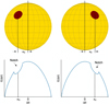 |
Fig. 1 Effect induced by the presence of a stellar spot on the rotational profile. Upper panel: Spot centred at (-x0,y0) on the projected stellar disc. The rotation of the star brings the spot centre to the new position on the disc (x0,y0). Bottom panel: Rotation profile modified by the presence of a spot. The Doppler-shift distribution exhibits a notch or dip at the spot’s position. As rotation carries the spot across the stellar disc, the position of the notch moves across the Doppler-shift distribution and its strength changes with the projected area of the spot and for the effect of the limb darkening. Figure adapted from Gray (2018). |
4 CCF correction
When the ‘objAB’ acquisition mode is employed for HARPS-N, the fibre B of the spectrograph is used to acquire the sky spectrum in order to obtain an optimal subtraction of the detector noise and background. The DRS pipeline also computes the CCF of the sky spectrum obtained using the fibre B, which we denote CCFB.
Some of the V1298 Tau CCF profiles that were analysed exhibited anomalous deformations that were also present in the CCFB (see an example in Fig. 2). These types of deformations could appear in the wings or even the core of the CCF profile, leading to incorrect RV estimations and/or the introduction of spurious signals. As previously reported by Malavolta et al. (2017), these deformations may be caused by moon illumination. To mitigate these deformations in all the CCF profiles, we followed the procedure described in Malavolta et al. (2017). Firstly, we recalculated the CCFB using the same flux-correction coefficients as those used for the target CCFA during the specific acquisition. Next, the CCFB was subtracted from the corresponding CCFA. The outcome of this process is the sky-corrected CCF profile (lower panel of Fig. 2).
5 Extraction of spot parameters and radial velocities
The CCF profiles of V1298 Tau, which are corrected for sky effects, exhibit multiple deformations as shown in Fig. 3.
We applied SpotCCF to the CCF profiles of V1298 Tau in two steps. In the first step, we used a model that accounted for the presence of one black spot on the stellar disc, which we refer to as the ‘One-spot model’. We explored the full (hyper)parameter space using the Monte Carlo (MC) nested sampler and Bayesian inference tool MultiNest v3.10 (Feroz et al. 2019), with the pyMutliNest wrapper (Buchner 2016). The priors used in all the analyses described below are summarised in Table 2. The MC sampler was set up to run with 5120 live points for both the One-spot model and the Two-spots (see below) model and with a sampling efficiency of 0.5 for all cases considered in this study.
The log-likelihood function to be minimised is expressed as:
![$\ln p\left( {{y_{\rm{n}}},{t_{\rm{n}}},\theta } \right) = - {1 \over 2}\sum\limits_{n = 1}^N {{{{{\left[ {{y_{\rm{n}}} - {f_\theta }\left( {{t_{\rm{n}}}} \right)} \right]}^2}} \over {{\sigma ^2}}}} - {1 \over 2}\ln \,\left[ {2\pi \left( {\sigma _{\rm{j}}^2} \right)} \right]{\rm{,}}$](/articles/aa/full_html/2024/03/aa48223-23/aa48223-23-eq17.png)
where yn and tn are the values of the CCF profile and the Doppler velocities, respectively; θ is the array of model parameters, fθ(t) is the model function, N are the number of CCF points, and σj is the white noise term (jitter).
In general, there are four parameters for the star (υ sin i, RV, γ, i), three parameters for each spot (latitude, longitude, Rspot), a normalisation parameter, and the jitter σj.
To establish the priors for the parameters υ sin i, γ, and i, which should be consistent across all observations, we conducted a series of tests in which we allowed these parameters to vary within a range around their literature values. In particular, we kept υ sin i fixed at 24.74 km s−1, which is the value most frequently obtained in previous tests, and the inclination of the rotation axis to the line of sight i at 90 degrees (a reasonable estimate derived from the value of υ sin i, R⋆ and Prot). Additionally, to break the degeneracy on the hemispheric location of the spots that arises when the inclination of the spin axis is 90 degrees, we assume that the spots are always located in the northern hemisphere of the star. This star is observed close to equator-on, such that a spot in the upper hemisphere – or symmetrically, in the lower hemisphere – of the star, with the same longitude and filling factor, contributes equally to the CCF profile. The spot radius, normalised to the stellar radius, was allowed to vary in the range [10−2, 0.5] to prevent spots that were too small from being resolved by the mapping resolution, or to prevent spots that are too large and cover the entire stellar surface.
In the second step, we used a model that accounts for the presence of two different black spots on the stellar surface (‘Two-spots model’) to fit the CCF. We note that this multi-spot model also considers cases where spots are entirely or partially overlapping. We adopted the same priors as in the One-spot model, which are detailed in Table 2. The logarithmic Bayesian evidence, log 𝒵, was used as an estimate of the goodness of the model. There is very strong evidence (Δ log 𝒵 ≈ 2000 >> 5) according to Kass-Raftery scale (Kass & Raftery 1995), supporting the Two-spots model for all the analysed CCF profiles of V1298Tau.
Figure 4 shows an example of a CCF profile of V1298 Tau fitted with a One-spot model and Two-spots model, and the corresponding spot configuration. As an example, Fig. 5 shows the corner plot of the best-fit parameters acquired from fitting a CCF profile of V1298 Tau using the Two-spots model. Here, σJ is the jitter noise, which refers to the noise level to be added to the model as an additional parameter to account for unmodelled contributions or other factors not considered by the model.
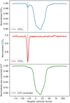 |
Fig. 2 Example of CCF profile distorted by the effect of the moon illumination. Top: CCF profile of the fibre A. (Middle) CCF profile of fibre B, CCFB. The black dashed vertical lines highlight the deformations in both profiles. Bottom: Sky-corrected CCF. |
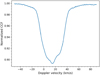 |
Fig. 3 Example of a normalised CCF profile of V1298 Tau. The deformed profile is due to the presence of one or multiple spots. |
Prior parameters of the model used for RV extraction of V1298 Tau.
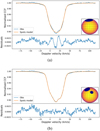 |
Fig. 4 Examples of CCF profiles of V1298 Tau fitted with One-spot model (a) and Two-spots model (b) and the corresponding residuals (in bottom panels). The inset of each plot shows the location of the spots on the stellar disc, as defined by the fit of both models; the grid indicates longitudes and latitudes from −90 to 90 degrees with 15-degree intervals. |
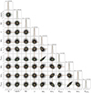 |
Fig. 5 Example corner plot of the best-fit parameters obtained from the fitting of a CCF profile of V1298 Tau with the Two-spots model. The red and green lines mark the median and the maximum a posteriori values, respectively, while the dashed black lines are the 16th and 84th quantiles. The median ± 1σ values are reported in the title of each histogram. The latitude and longitude scales are in radians. |
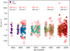 |
Fig. 6 Comparison between RV measurements obtained with the SpotCCF (coloured filled points, ranging from blue to red as a function of the observation time) and TERRA RVs (red empty points). For each season, we indicate the RMS of the corresponding RV subsample: the RMS of the RVs extracted from TERRA in red, and the RMS of the SpotCCF RVs in black. |
6 Radial velocity time-series analysis
To extract the RVs of V1298 Tau, we applied SpotCCF to its CCF profiles, selecting the best model based on Bayesian evidence values, typically the Two-spots model. We compared the RV time series obtained with SpotCCF to the RVs obtained with the TERRA pipeline (see Fig. 6), as the latter shows a reduced RV dispersion compared to the DRS. The root mean square (RMS) of the RVs obtained with SpotCCF is significantly smaller (between 40% and 60%) than the RMS obtained with TERRA, with the largest decrease observed during the second season. In addition, we assessed the effect of including an extra spot in the SpotCCF model (Three-spots model) on the extraction of RVs. We verified that the Three-spots model exhibited greater RV dispersion compared to the Two-spots model in all observing seasons. This can be attributed to correlations between the RV measurements and the other parameters, such as γ or the longitudes of the third spot, correlations that were not present in the Two-spots model (see an example in Figs. B.1 and B.2).
To search for periodicities in the RV data obtained with SpotCCF, we used the generalized Lomb-Scargle periodogram (GLS, Zechmeister & Kürster 2009). The periodogram (see Fig. 7a) identifies a significant frequency at 0.34716 ± 0.00005 day−1 (period of 2.8806 ± 0.0004 days), corresponding to the rotational period of the star, Prot, highlighted with a dashed magenta line, and the 1 − f alias (frequency of about 0.65 day−1). Figure 7a shows the periodogram of the RVs obtained with the TERRA pipeline. In this case, as well, the periodogram identifies a significant frequency at the Prot of the star. However, the frequency at the first harmonic of the Prot of the star (green dashed line), which is present in the TERRA periodogram, disappears in the SpotCCF periodogram. Furthermore, it is worth noting that the SpotCCF periodogram does not reveal the intricate pattern of peaks around the Prot and its harmonics, respectively, which are clearly visible in the TERRA periodogram. The results of the sinusoidal fit from both periodograms are summarised in Table 3.
We note that the RV semi-amplitude obtained from SpotCCF is about 30% lower than the one obtained with TERRA, and the RMS of the residuals obtained from the subtraction of the best sinusoid from SpotCCF RVs is about 45% lower than the TERRA RMS of the residuals. Furthermore, it can be noted that the modulation present in the phase-folded residuals of TERRA disappears when SpotCCF is used (see the bottom right panel in Figs. 7a and b). This is also confirmed by the periodogram, as the SpotCCF periodogram appears cleaner and the rotational period seems better identified. This result suggests a substantial removal of rotation-related frequencies by SpotCCF. The presence of a peak at the Prot that remains visible could be attributed to the approximate representation of spots, both in terms of their number and shape, within the SpotCCF model, or to other phenomena responsible of the stellar variations.
We performed an additional test by calculating the GLS periodograms for both the original data and residuals obtained after recursive prewhitening for both datasets. The periodogram of TERRA RVs exhibits a complex structure centred around the stellar rotation frequency, with signals related to the stellar activity (at the rotational frequency or its harmonics) prominently dominating the periodograms even after four iterations of prewhitening. However, the periodogram of the SpotCCF RVs does not display harmonics of the rotation frequency, and the signal at the stellar rotational frequency disappears after the second prewhitening step (see Fig. 8). Our analysis strongly supports a conclusion that the SpotCCF model efficiently removes part of the contribution from the stellar activity related to the rotation.
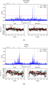 |
Fig. 7 GLS periodogram of the V1298 Tau RVs obtained with the SpotCCF (panel a) and the TERRA pipeline (panel b). The red dots highlight the maximum power and the dashed red line indicates the FAP at 1.0% (upper panels). The vertical dashed magenta line highlights the Prot of the star, while the green dashed line indicates Prot/2. The bottom panels show the RVs (left) and the residuals (right) phase folded with the dominant period. The colour gradient, as shown in Fig. 6, helps in identifying the modulation in the phase-fold residuals across different observing seasons. |
Summary of the sinusoidal fits obtained from the periodograms applied to the V1298 Tau RVs derived with SpotCCF and TERRA.
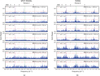 |
Fig. 8 GLS periodogram of the V1298 Tau RVs obtained with the SpotCCF (panel a) and the TERRA (panel b) pipeline and their residuals after recursive prewhitening. In each panel, the vertical and dashed lines indicate the stellar rotation frequency (in magenta) and its harmonics (in green and black), and the horizontal red dashed line highlights the FAP at 1.0%. Each panel reports the RMS of the dataset. |
7 Spot characterisation
The fit of the CCFs profile with SpotCCF allows characterisation of the spots present on the stellar surface. In particular, latitude and longitude provide the position of the spot, while the projected filling factor (ffp) suggests its size (see Table B.1).
From a preliminary analysis, we decided to make the raw assumption that the spot system consists of a larger (Spot A) and a smaller (Spot B) spot evolving separately.
Figure 9 shows the relation between the latitude of the spots and the projected filling factor obtained for V1298 Tau, and the respective distributions (see the histograms on the top and right side of the main plot). According to our assumption, we find an indication of two main peaks, with larger spots (ffp > 0.06) preferentially in the range of ≈45–90 degrees, and smaller spots (ffp < 0.02) in the range of 0–10 degrees. The linear upper envelope that characterises the larger spots is attributable to the upper limit of the spot radius boundary.
We performed the GLS periodogram analysis of longitudes and projected filling factor obtained for V1298 Tau. The upper panel of Fig. 10 shows the longitude time series for Spot A and Spot B in blue and orange, respectively, and the lower panels show the GLS periodograms performed for each spot. A significant peak at 2.91 days, near the rotational period of the star, is identified for Spot A with a false alarm probability (FAP) of ≤0.1%, while a significant peak (FAP ≤ 10%) at 2.77 days is identified for Spot B.
The GLS periodogram of the projected filling factor of the two spot distributions is shown in Fig. 11. Even in this case, a significant peak (FAP ≤ 1%) is identified for Spot A at 2.91 days, while Spot B shows a lower significant peak (FAP ≈ 10%, 2.84 days).
Both periodogram analyses indicate that the deformations in the CCF profiles are modulated with the stellar rotation, confirming our hypothesis that these deformations are caused by the presence of stellar spots rotating solidly with the star.
The lower significance of the peaks observed for Spot B is not surprising, as Spot A is larger and therefore contributes more significantly to the CCF profile, making it easier to detect. However, as Spot B is smaller, when there are more than two spots on the stellar surface or when a simplistic description of a circular spot is not sufficient, there can be multiple configurations for Spot B. Furthermore, the definition of ‘large’ and ‘small’ spots are not strictly defined and are relative to the specific configuration, as there can be cases where both spots should be categorised as large, but one is slightly smaller than the other, though still falling within the small category.
Furthermore, we analysed the total area covered by the spots,  , which was obtained by summing up the ffp of each individual spot. The upper panel of Fig. 12 shows the
  times-series.
It is worth noting that the range of the total projected filling factor obtained for V1298 Tau is consistent with the value proposed by Messina et al. (2001), according to which a star like V1298 Tau, with a rotational period of about 3 days, has approximately 15% of its surface covered by spots.
The GLS periodogram of the  time series reveals a peak corresponding to the second harmonic of the Prot of the star (FAP ≤ 10%). As we are monitoring the total area covered by the spot, the presence of peaks at both Prot and Prot /2 indicates a non-uniform spot distribution concentrated along two distinct mean longitudes separated by 180 degrees. Moreover, the different power of these peaks suggests that these two opposing spot distributions cover different areas on the stellar surface. This behaviour appears to remain fairly stable over time.
As a further validation of the method, we compare the spot configuration of observations obtained on the same nights. Figure C.1 presents the spot configurations obtained from pairs of observations taken at very few hours of separation. Specifically, we compare the spot configurations obtained from observations taken during the same night, but a few hours apart. It is important to note that each observation was analysed independently, and obtaining the same configuration of spots on the same night (with very few exceptions on 16 January 2023 and 17 January 2023) serves as confirmation of the reliability of the method.
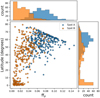 |
Fig. 9 Relationship between latitude and ffp for spots on V1298 Tau. Blue points represent the spot with the highest ffp (Spot A), while orange points correspond to spots with the lowest ffp (Spot B). The histograms on the top and right side of the main plot depict the distributions of latitudes and ffp, respectively. |
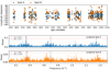 |
Fig. 10 V1298 Tau longitudes time-series (upper panel). The blue points indicate the large spots (Spot A), while the orange points are the small spots (Spot B). GLS periodogram performed for the longitude values obtained for Spot A and Spot B, respectively (lower panels). The red horizontal line indicates the FAP level at 0.1% and 10%, respectively. The black dashed lines highlight the rotational period of the star and its harmonic. |
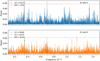 |
Fig. 11 GLS periodogram of the projected filling factor of Spot A (upper panel) and Spot B (lower panel). The red horizontal line indicates the FAP level at 1% and 10%, respectively. The black dashed lines highlight the rotational period of the star and its harmonic. |
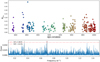 |
Fig. 12 Total projected filling factor time series of V1298 Tau (upper panel) and corresponding GLS periodogram (lower panel). The points are coloured following a colour scale from blue to red as a function of the observation time. The red horizontal line in the periodogram indicates the FAP level at 10%, while the black dashed lines highlight the rotational period of the star and its harmonic. |
8 Differential stellar rotation
To test the presence of differential rotation, we categorised the spots into two groups: larger spots located between latitudes of 60 and 90 degrees (referred as Spot A at ≥ 60°), and smaller spots located between latitudes of 0 and 40 degrees (Spot B at ≤ 40°). This eliminates the small spots at high latitudes. Figure 13 illustrates this new selection, depicting the distribution of latitude as a function of the ffp.
The GLS periodogram was performed on the projected filling factor distribution of the two spots (see Fig. 14). The analysis reveals a significant peak (FAP ≤ 1%) for Spot A and Spot B, at periods of 3.24 and 2.53 days, respectively. These periods may provide a suggestion of a differential rotational velocity of the star, with a higher velocity at lower latitudes (P = 2.53 days close to the equator) and lower rotational velocity at higher latitudes (P = 3.24 days close to the pole). Additionally, it can be observed that the peak at 3.24 days is one of the peaks near the rotational period of the star in the TERRA periodogram, which was removed by the SpotCCF method.
9 Detection sensitivity by direct injection of the planetary signal into the data
In order to obtain further validation of the SpotCCF method, we tested the ability to recover the planetary signal in the time series of V1298 Tau. For this purpose, we created different datasets by injecting a planetary signal with an orbital period of 4.9 days2 and using different amplitudes (K = 37, 75, 100, 150 ms−1) in the RV dataset obtained with SpotCCF and with the TERRA pipeline, respectively. Before proceeding, we tested the reliability of the method by injecting the signal on the CCFs verifying that the two procedures give the same RV. To simulate a planetary signal, the CCFs were blue or redshifted with the desired amplitude, period, and phase. We performed the fit for all the shifted CCFs and the results are compatible with the fit obtained with the original CCFs. For this reason, and given that the fit of CCFs is computationally demanding, we chose to inject the planetary signal directly on the original RVs time series.
The GLS periodogram was computed for each dataset. Figure 15 shows the comparison between the periodograms of the RVs+planet (injected at different amplitude) obtained from the original SpotCCF RVs (left panel) and from the original TERRA dataset (right panel). In both datasets (SpotCCF and TERRA), the GLS periodogram finds a significant peak at the rotational period of the star. The second row of the figure shows the periodogram for the RVs with the planet injection at different amplitudes.
The GLS periodogram finds a significant peak (FAP < 1.0%) at the orbital period of the injected planet with K ≈ 37 m s−1 (corresponding to M sin i ≈ 0.35 MJ) for the RVs obtained with SpotCCF. An analogous peak is significant for the TERRA RVs only for an injected planet with K ≈ 75 m s−1 (corresponding to M sin i ≈ 0.70 MJ).
This test suggests that this method can be used to reliably detect a lower-mass planet with an amplitude of the injected signal lower than what is required for the signal to be identified in the TERRA dataset. This result is consistent with the finding that the SpotCCF model reduces systematic effects caused by stellar activity.
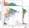 |
Fig. 13 Relationship between latitude and ffp. The histograms on the top and right side of the main plot depict the distributions of latitudes and ffp, respectively. Blue points represent the spot with the highest ffp (Spot A), while orange points indicate the spots with the lowest ffp (Spot B). Purple points and distribution represent Spot B with latitude values lower than 40 degrees, while green points and distribution indicate Spot A with latitude values higher than 60 degrees. |
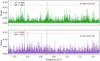 |
Fig. 14 GLS periodogram of the projected filling factor of Spot A with a latitude higher than 60 degrees (upper panel) and Spot B with a latitude lower than 40 degrees (lower panel). The red horizontal line indicates the FAP level at 1%. The black dashed lines highlight the rotational period of the star and its harmonic. |
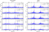 |
Fig. 15 Comparison between the GLS periodograms of the V1298 Tau RVs obtained with the SpotCCF (left panels) and the TERRA pipeline (right panels) where we injected a planetary signal at Porb = 4.9 d, with different amplitude (from top to bottom K = 0, 37, 75, 100, 150 m s−1). The vertical and dashed black lines indicate the stellar rotation frequency and its harmonics; the green line marks the orbital frequency of the injected planet, while the red dashed horizontal line highlights the FAP at 1.0%. The upper panel shows the original dataset without planet injection. |
10 Discussion and conclusions
In this work, we describe SpotCCF, a stellar photosphere model fit. SpotCCF is able to extract the spot configuration of the star and also optimise the RV extraction in young, active stars based on the CCF technique. This model takes into account the deformations of the CCF due to the presence of multiple spots on the stellar disc in the presence of significant rotation.
To test the validity of our model, we analysed V1298 Tau HARPS-N observations, which exhibit distorted CCF profiles due to the high-activity level of this target. The original CCF profiles produced by the DRS pipeline were corrected for anomalous deformations present in the wings and in the core of the line, as well as in the CCFB of the sky spectrum obtained using fibre B.
We then analysed over 300 HARPS-N observations of V1298 Tau using a model with multiple spots, referred to here as the Two-spots model. From the parameters through the fit performed on the CCF profiles, we extracted information about the spots, including latitude, longitude, and the area covered by each spot. We found two main distributions with polar or high-latitude spots, in agreement with the high rotation of the star, and smaller low-latitude spots (e.g, Barnes et al. 2001; Strassmeier 2002; Cang et al. 2021). To analyse the spot properties, we separated the high-latitude spots (Spot A, ffp ≥ 0.04 and latitude > 60°) from the smaller, low-latitude spots (Spot B, ffp < 0.04 and latitude ≤50°). Under this assumption, the GLS periodogram of the filling factor of Spot A and Spot B showed significant peaks (FAP ≤ 1%) at 3.24 and 2.53 days, respectively, suggesting a solar-like differential rotation of the star, α = (Ωeq − Ωpol)/Ωeq ≃ 0.2 (α⊙ = 0.2; Balona & Abedigamba 2016), with lower rotation at higher latitudes. This estimate places this target in the uppermost region of Fig. 11 provided by Reinhold et al. (2013), confirming the extreme behaviour of this star.
The average total area covered by the spots is consistent with the range proposed by Messina et al. (2001). The GLS periodogram of the total projected filling factor,  , showed a significant peak at the Prot/2 with a FAP ≤ 10%, indicating that the features identified in the CCF profiles are effects due to a few inhomogeneities (spots) on opposite hemispheres of the stellar surface modulated by the rotation. The consistency of the spot configuration obtained from different observations taken during the same night – but a few hours apart – confirms the reliability of the method.
Moreover, our results are consistent with the spot configuration of V1298 Tau obtained by Morris (2020). In that paper, the author modelled the ‘K2 Campaign 4’ light curves of V1298 Tau, identifying a three-spot configuration. Two main spots were located in the range of 60-90 degrees (northern hemisphere, NH) and 30–60 degrees (southern hemisphere, SH), respectively, while a smaller spot was positioned at lower latitudes (0–30 NH). A starspot-covered fraction, fs, was estimated at  , per cent. The observed spot configuration aligns with our two spot distributions, featuring a larger spot up to 60 degrees and a smaller one in the range of 0–40 degrees. The total projected filling factor of V1298 Tau estimated using SpotCCF is consistent with the estimation of these latter authors. The median value of
  of 0.06 ± 0.04 obtained by SpotCCF considers only the spot coverage of the visible hemisphere, representing half of the fs estimated by Morris (2020).
The SpotCCF model applied to the HARPS-N observations of V1298 Tau enables a reduction of the effect of the contribution of stellar activity on RVs measurements. We compared these RVs with those obtained using the TERRA pipeline to highlight the benefits of the proposed method. We observe that the RVs obtained with SpotCCF model show lower dispersion, with a decrease ranging from 40% to 60% in each season, compared to the TERRA dataset. Additionally, a search for periodicities in the RV dataset revealed a significant peak at the rotational period of the star, with reduced RV amplitude for the SpotCCF RVs (about 30% lower than those obtained with TERRA) and reduced dispersion in the residuals. These results suggest that our new method for RV extraction partially mitigates the contribution of stellar activity modulated with stellar rotation. This conclusion is further supported by the GLS periodogram performed on the SpotCCF dataset and on its residuals obtained after recursive prewhitening, which show the removal of the peak at the harmonics of the rotation after the first prewhitening, while they are still present in the periodogram of the TERRA dataset. These results, particularly the significant peak at Prot persisting even after SpotCCF modelling, imply that stellar variations are not fully explained by the existence of two prominent spots on the stellar surface alone. The variability observed in the original RV time series results not only from the presence of these two major spots but also from additional factors not accounted for in the model. These factors may include phenomena like the presence of plages or unmodelled spots that are smaller than those significantly impacting the CCF profile. Additionally, there may be unmodelled effects associated with larger spots, such as the inhibition of convection, leading to changes in the convection blueshift when the spots are visible (Cavallini et al. 1985; Dravins et al. 1981; Meunier et al. 2015, 2017). We also tested the detection sensitivity of the method by directly injecting a hypothetical planetary signal (Porb = 4.9 days) into the data. The results obtained from the GLS periodogram suggest that the RV times series obtained with the SpotCCF method allows the reliable detection of a planet with a lower-amplitude signal (K ≈ 37 m s−1) than that necessary for identification in the TERRA dataset (K ≥ 75 m s−1).
All the results of this work confirm that the developed method can extract information about the spot configuration of the star and also optimise RV extraction in young and active stars, improving detection sensitivity and our ability to recover planetary signals, and reducing the probability of identifying signals that are due to stellar activity but can be mistaken as planetary signals.
We plan to apply the method proposed in the present work to other targets that exhibit high values of v sin i in order to assess the applicability range of the model. Furthermore, we could apply the SpotCCF model to the single spectral lines that are predominantly affected by rotational broadening and are distorted by the presence of spots in order to more accurately characterise the line profiles.
Acknowledgements
We thank the anonymous referee for her/his helpful comments and suggestions. We acknowledge partial support of Ariel ASI-INAF agreement no. 2021-5-HH.0. We acknowledge PRACE for awarding access to the Fenix Infrastructure resources at CINECA, which are partially funded from the European Union's Horizon 2020 research and innovation programme through the ICEI project under the grant agreement no. 800858. We also acknowledge the computing infrastructure PLEIADI, INAF – USC VIII, for the availability of HPC resources. The research activities described in this paper were carried out with contribution of the Next Generation EU funds within the National Recovery and Resilience Plan (PNRR), Mission 4 – Education and Research, Component 2 - From Research to Business (M4C2), Investment Line 3.1 – Strengthening and creation of Research Infrastructures, Project IR0000034 – “STILES – Strengthening the Italian Leadership in ELT and SKA”.
Appendix A Spot model
Let us consider a Cartesian orthogonal reference frame with its origin in the barycentre of the star O and the Z axis along the stellar spin axis. The XY plane is defined in such a way as to contain the line of sight, indicated as  (see Figure A.1).
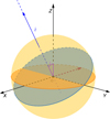 |
Fig. A.1 OXYZ reference frame with its origin in the barycentre O of the star, the Z axis along the stellar spin axis Ω⋆, and the XZ plane oriented as to contain the line of sight |

Indicating the latitude and the longitude of a point P on the surface of the star with (ϕ,λ), it has the Cartesian coordinate

where R⋆ is the radius of the star assumed to be spherically symmetric. In our fixed reference frame, the longitude λ is increasing over time t because of stellar rotation; it changes according to

where λ0 is the longitude at the initial time t0 and Ω⋆ = 2π/Prot is the stellar angular velocity of rotation with Prot the rotation period.
To obtain the coordinates in the reference frame adopted in this work, we first make a rotation of the angle i around the Y axis, where i is the inclination of the stellar spin to the line of sight z. This brings the XY plane in the plane of the sky which is the same plane of the stellar disc. The equations of such a rotation are


This gives


The unit vector along the spin axis of the star in the OXYZ reference frame is  . Transforming it to the Oxyz reference frame, it becomes (− sin i, 0, cos i). As the z axis is directed along the line of sight, the projection of the spin axis onto the plane of the sky xy, that is, the plane of the stellar disc, is (− sin i, 0). The reference frame adopted in the model to describe the disc of the star has the x0 axis orthogonal to the projection of the spin axis on the plane of the sky and the y0 axis along that projection. This implies that our x0 = y and y0 = −x because the projection of the spin axis in the plane of the stellar disc is opposite to the orientation of our x-axis, given that its component along our x axis is − sin i < 0 for 0° ≤ i ≤ 180°.
In conclusion, we find


Appendix B Spot distribution
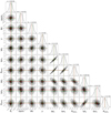 |
Fig. B.1 Example corner plot of the best-fit parameters obtained from the fitting of a CCF profile of V1298 Tau with the Two-spots model. The red and green lines mark the median and the maximum-a posteriori values, respectively, while the dashed black lines are the 16th and 84th quantiles. The median ± 1σ values are reported in the title of each histogram. The latitude and longitude scales are in radians. log Z = 31005 |
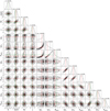 |
Fig. B.2 Example corner plot of the best-fit parameters obtained from the fitting of a CCF profile of V1298 Tau with the Three-spots model. We can also note that the distributions obtained for the third spot (latitude, longitude, and radius) are not well constrained. log Z = 31156 |
Spot parameters derived by the Two-spots model.
Appendix C Spot configuration for the same night of observations
 |
Fig. C.1 Spot configuration of pairs of observations obtained at a few hours of distance. Each map shows the results obtained by the chain. At each step, the chain generates a map for each triplet of values (latitude, longitude, and radius), drawing the corresponding spot on the stellar surface. The final map, as well as those shown in this figure, is obtained by summing the individual maps obtained at each step of the chain using a colour scale ranging from red to blue. The bluest area on the map represents the final configuration of each spot determined by the chain. |
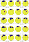 |
Fig. C.2 Spot configuration of pairs of observations obtained at a few hours of distance (continued). |
References
- Anglada-Escudé, G., & Butler, R. P. 2012, ApJS, 200, 15 [Google Scholar]
- Arlt, R., & Rüdiger, G. 2011, MNRAS, 412, 107 [NASA ADS] [CrossRef] [Google Scholar]
- Balona, L. A., & Abedigamba, O. P. 2016, MNRAS, 461, 497 [NASA ADS] [CrossRef] [Google Scholar]
- Baranne, A., Queloz, D., Mayor, M., et al. 1996, A&AS, 119, 373 [NASA ADS] [CrossRef] [EDP Sciences] [Google Scholar]
- Barnes, J. R., Collier Cameron, A., James, D. J., & Steeghs, D. 2001, MNRAS, 326, 1057 [NASA ADS] [CrossRef] [Google Scholar]
- Beichman, C., Hirano, T., David, T. J., et al. 2019, RNAAS, 3, 89 [NASA ADS] [Google Scholar]
- Buchner, J. 2016, Astrophysics Source Code Library [record ascl:1606.005] [Google Scholar]
- Budding, E. 1977, Ap&SS, 48, 207 [NASA ADS] [CrossRef] [Google Scholar]
- Cang, T. Q., Petit, P., Donati, J. F., & Folsom, C. P. 2021, A&A, 654, A42 [NASA ADS] [CrossRef] [EDP Sciences] [Google Scholar]
- Carleo, I., Malavolta, L., Lanza, A. F., et al. 2020, A&A, 638, A5 [NASA ADS] [CrossRef] [EDP Sciences] [Google Scholar]
- Cavallini, F., Ceppatelli, G., & Righini, A. 1985, A&A, 143, 116 [NASA ADS] [Google Scholar]
- Choudhuri, A. R. 2017, Sci. China Phys. Mech. Astron., 60, 19601 [NASA ADS] [CrossRef] [Google Scholar]
- Claret, A. 2000, A&A, 363, 1081 [NASA ADS] [Google Scholar]
- Claret, A., Hauschildt, P. H., & Witte, S. 2012, A&A, 546, A14 [NASA ADS] [CrossRef] [EDP Sciences] [Google Scholar]
- Claret, A., Hauschildt, P. H., & Witte, S. 2013, A&A, 552, A16 [NASA ADS] [CrossRef] [EDP Sciences] [Google Scholar]
- Collier Cameron, A., & Unruh, Y. C. 1994, MNRAS, 269, 814 [NASA ADS] [CrossRef] [Google Scholar]
- Cosentino, R., Lovis, C., Pepe, F., et al. 2014, SPIE Conf. Ser., 9147, 91478C [Google Scholar]
- Covino, E., Esposito, M., Barbieri, M., et al. 2013, A&A, 554, A28 [NASA ADS] [CrossRef] [EDP Sciences] [Google Scholar]
- Cretignier, M., Dumusque, X., Allart, R., Pepe, F., & Lovis, C. 2020, A&A, 633, A76 [NASA ADS] [CrossRef] [EDP Sciences] [Google Scholar]
- Damasso, M., Locci, D., Benatti, S., et al. 2023, A&A, 672, A126 [NASA ADS] [CrossRef] [EDP Sciences] [Google Scholar]
- Davenport, J. R. A. 2016, ApJ, 829, 23 [Google Scholar]
- David, T. J., Cody, A. M., Hedges, C. L., et al. 2019a, AJ, 158, 79 [NASA ADS] [CrossRef] [Google Scholar]
- David, T. J., Petigura, E. A., Luger, R., et al. 2019b, ApJ, 885, L12 [Google Scholar]
- Desert, J.-M., Adhiambo, V., Barat, S., et al. 2021, The nature, origin, and fate of two planets of a newborn system through the lens of their relative atmospheric properties, JWST Proposal. Cycle 1, 2149 [Google Scholar]
- Di Maio, C., Argiroffi, C., Micela, G., et al. 2020, A&A, 642, A53 [NASA ADS] [CrossRef] [EDP Sciences] [Google Scholar]
- Donati, J. F., Collier Cameron, A., Hussain, G. A. J., & Semel, M. 1998, ASP Conf. Ser., 154, 1966 [NASA ADS] [Google Scholar]
- Donati, J. F., Collier Cameron, A., Semel, M., et al. 2003, MNRAS, 345, 1145 [NASA ADS] [CrossRef] [Google Scholar]
- Dravins, D., Lindegren, L., & Nordlund, A. 1981, A&A, 96, 345 [NASA ADS] [Google Scholar]
- Dumusque, X. 2018, A&A, 620, A47 [NASA ADS] [CrossRef] [EDP Sciences] [Google Scholar]
- Dumusque, X., Cretignier, M., Sosnowska, D., et al. 2021, A&A, 648, A103 [NASA ADS] [CrossRef] [EDP Sciences] [Google Scholar]
- Feinstein, A. D., Montet, B. T., Johnson, M. C., et al. 2021, AJ, 162, 213 [NASA ADS] [CrossRef] [Google Scholar]
- Feinstein, A. D., David, T. J., Montet, B. T., et al. 2022, ApJ, 925, L2 [NASA ADS] [CrossRef] [Google Scholar]
- Fellgett, P. 1955, Optica Acta, 2, 9 [NASA ADS] [CrossRef] [Google Scholar]
- Feroz, F., Hobson, M. P., Cameron, E., & Pettitt, A. N. 2019, Open J. Astrophys., 2, 10 [Google Scholar]
- Finociety, B., Donati, J. F., Cristofari, P. I., et al. 2023, MNRAS, 526, 4627 [NASA ADS] [CrossRef] [Google Scholar]
- Gaia Collaboration (Brown, A. G. A., et al.) 2021, A&A, 649, A1 [NASA ADS] [CrossRef] [EDP Sciences] [Google Scholar]
- Gaidos, E., Hirano, T., Beichman, C., et al. 2022, MNRAS, 509, 2969 [Google Scholar]
- Gray, D. F. 2018, ApJ, 857, 139 [NASA ADS] [CrossRef] [Google Scholar]
- Haywood, R. D., Collier Cameron, A., Queloz, D., et al. 2014, MNRAS, 443, 2517 [Google Scholar]
- He, H., Wang, H., Zhang, M., et al. 2018, ApJS, 236, 7 [Google Scholar]
- Howarth, I. D. 2011, MNRAS, 413, 1515 [NASA ADS] [CrossRef] [Google Scholar]
- Howell, S. B., Sobeck, C., Haas, M., et al. 2014, PASP, 126, 398 [Google Scholar]
- Hunter, A., Macgregor, A., Szabo, T., Wellington, C., & Bellgard, M. 2012, Source Code Biol. Med., 7, 1 [Google Scholar]
- Johnson, M. C., David, T. J., Petigura, E. A., et al. 2022, AJ, 163, 247 [NASA ADS] [CrossRef] [Google Scholar]
- Kass, R. E., & Raftery, A. E. 1995, J. Am. Stat. Assoc., 90, 773 [Google Scholar]
- Kitchatinov, L. L., & Olemskoy, S. V. 2015, Res. Astron. Astrophys., 15, 1801 [Google Scholar]
- Kron, G. E. 1947, PASP, 59, 261 [NASA ADS] [CrossRef] [Google Scholar]
- Lanza, A. F. 2016, in Lect. Notes Phys., 914 (Berlin: Springer Verlag), eds. J.-P. Rozelot, & C. Neiner, 43 [NASA ADS] [CrossRef] [Google Scholar]
- Lanza, A. F., Bonomo, A. S., Moutou, C., et al. 2010, A&A, 520, A53 [NASA ADS] [CrossRef] [EDP Sciences] [Google Scholar]
- Lanza, A. F., Malavolta, L., Benatti, S., et al. 2018, A&A, 616, A155 [NASA ADS] [CrossRef] [EDP Sciences] [Google Scholar]
- Maggio, A., Locci, D., Pillitteri, I., et al. 2022, ApJ, 925, 172 [NASA ADS] [CrossRef] [Google Scholar]
- Malavolta, L., Borsato, L., Granata, V., et al. 2017, AJ, 153, 224 [NASA ADS] [CrossRef] [Google Scholar]
- Maldonado, J., Scandariato, G., Stelzer, B., et al. 2017, A&A, 598, A27 [NASA ADS] [CrossRef] [EDP Sciences] [Google Scholar]
- Maldonado, J., Phillips, D. F., Dumusque, X., et al. 2019, A&A, 627, A118 [NASA ADS] [CrossRef] [EDP Sciences] [Google Scholar]
- Mancini, L., Southworth, J., Raia, G., et al. 2017, MNRAS, 465, 843 [NASA ADS] [CrossRef] [Google Scholar]
- Messina, S., Rodonò, M., & Guinan, E. F. 2001, A&A, 366, 215 [NASA ADS] [CrossRef] [EDP Sciences] [Google Scholar]
- Meunier, N., & Lagrange, A. M. 2020, A&A, 638, A54 [NASA ADS] [CrossRef] [EDP Sciences] [Google Scholar]
- Meunier, N., Desort, M., & Lagrange, A. M. 2010, A&A, 512, A39 [NASA ADS] [CrossRef] [EDP Sciences] [Google Scholar]
- Meunier, N., Lagrange, A. M., Borgniet, S., & Rieutord, M. 2015, A&A, 583, A118 [NASA ADS] [CrossRef] [EDP Sciences] [Google Scholar]
- Meunier, N., Lagrange, A. M., & Borgniet, S. 2017, A&A, 607, A6 [NASA ADS] [CrossRef] [EDP Sciences] [Google Scholar]
- Morello, G., Tsiaras, A., Howarth, I. D., & Homeier, D. 2017, AJ, 154, 111 [NASA ADS] [CrossRef] [Google Scholar]
- Morello, G., Claret, A., Martin-Lagarde, M., et al. 2020, AJ, 159, 75 [NASA ADS] [CrossRef] [Google Scholar]
- Morris, B. M. 2020, ApJ, 893, 67 [Google Scholar]
- Mosser, B., Baudin, F., Lanza, A. F., et al. 2009, A&A, 506, 245 [NASA ADS] [CrossRef] [EDP Sciences] [Google Scholar]
- Noyes, R. W., Hartmann, L. W., Baliunas, S. L., Duncan, D. K., & Vaughan, A. H. 1984, ApJ, 279, 763 [Google Scholar]
- Oh, S., Price-Whelan, A. M., Hogg, D. W., Morton, T. D., & Spergel, D. N. 2017, AJ, 153, 257 [NASA ADS] [CrossRef] [Google Scholar]
- Owen, J. E. 2020, MNRAS, 498, 5030 [Google Scholar]
- Pepe, F., Mayor, M., Galland, F., et al. 2002, A&A, 388, 632 [NASA ADS] [CrossRef] [EDP Sciences] [Google Scholar]
- Pizzolato, N., Maggio, A., Micela, G., Sciortino, S., & Ventura, P. 2003, A&A, 397, 147 [NASA ADS] [CrossRef] [EDP Sciences] [Google Scholar]
- Poppenhaeger, K., Ketzer, L., & Mallonn, M. 2021, MNRAS, 500, 4560 [Google Scholar]
- Rajpaul, V., Aigrain, S., Osborne, M. A., Reece, S., & Roberts, S. 2015, MNRAS, 452, 2269 [Google Scholar]
- Reinhold, T., Reiners, A., & Basri, G. 2013, A&A, 560, A4 [NASA ADS] [CrossRef] [EDP Sciences] [Google Scholar]
- Saar, S. H., & Fischer, D. 2000, ApJ, 534, L105 [NASA ADS] [CrossRef] [Google Scholar]
- Savanov, I. S., & Strassmeier, K. G. 2008, Astron. Nachr., 329, 364 [NASA ADS] [CrossRef] [Google Scholar]
- Scandariato, G., Maldonado, J., Affer, L., et al. 2017a, A&A, 598, A28 [NASA ADS] [CrossRef] [EDP Sciences] [Google Scholar]
- Scandariato, G., Nascimbeni, V., Lanza, A. F., et al. 2017b, A&A, 606, A134 [NASA ADS] [CrossRef] [EDP Sciences] [Google Scholar]
- Schlawin, E., Ilyin, I., Feinstein, A. D., et al. 2021, RNAAS, 5, 195 [NASA ADS] [Google Scholar]
- Schrijver, C. J., Cote, J., Zwaan, C., & Saar, S. H. 1989, ApJ, 337, 964 [NASA ADS] [CrossRef] [Google Scholar]
- See, V., Matt, S. P., Folsom, C. P., et al. 2019, ApJ, 876, 118 [Google Scholar]
- Skumanich, A., Smythe, C., & Frazier, E. N. 1975, ApJ, 200, 747 [Google Scholar]
- Solanki, S. K., Inhester, B., & Schüssler, M. 2006, Rep. Progr. Phys., 69, 563 [CrossRef] [Google Scholar]
- Spruit, H. C. 2002, A&A, 381, 923 [CrossRef] [EDP Sciences] [Google Scholar]
- Strassmeier, K. G. 2002, Astron. Nachr., 323, 309 [NASA ADS] [CrossRef] [Google Scholar]
- Strassmeier, K. G. 2009, A&A Rev., 17, 251 [NASA ADS] [CrossRef] [Google Scholar]
- Strassmeier, K. G., & Rice, J. B. 2000, A&A, 360, 1019 [NASA ADS] [Google Scholar]
- Strassmeier, K. G., Carroll, T. A., & Ilyin, I. V. 2023, A&A, 674, A118 [NASA ADS] [CrossRef] [EDP Sciences] [Google Scholar]
- Suárez Mascareño, A., Damasso, M., Lodieu, N., et al. 2021, Nat. Astron., 6, 232 [Google Scholar]
- Vidotto, A. A., Gregory, S. G., Jardine, M., et al. 2014, MNRAS, 441, 2361 [Google Scholar]
- Vissapragada, S., Stefánsson, G., Greklek-McKeon, M., et al. 2021, AJ, 162, 222 [NASA ADS] [CrossRef] [Google Scholar]
- Walkowicz, L. M., Basri, G., & Valenti, J. A. 2013, ApJS, 205, 17 [NASA ADS] [CrossRef] [Google Scholar]
- Wright, N. J., Drake, J. J., Mamajek, E. E., & Henry, G. W. 2011, ApJ, 743, 48 [Google Scholar]
- Zechmeister, M., & Kürster, M. 2009, A&A, 496, 577 [CrossRef] [EDP Sciences] [Google Scholar]
- Zhao, J., & Tinney, C. G. 2019, MNRAS, 491, 4131 [Google Scholar]
All Tables
Summary of the sinusoidal fits obtained from the periodograms applied to the V1298 Tau RVs derived with SpotCCF and TERRA.
All Figures
|
Fig. 1 Effect induced by the presence of a stellar spot on the rotational profile. Upper panel: Spot centred at (-x0,y0) on the projected stellar disc. The rotation of the star brings the spot centre to the new position on the disc (x0,y0). Bottom panel: Rotation profile modified by the presence of a spot. The Doppler-shift distribution exhibits a notch or dip at the spot’s position. As rotation carries the spot across the stellar disc, the position of the notch moves across the Doppler-shift distribution and its strength changes with the projected area of the spot and for the effect of the limb darkening. Figure adapted from Gray (2018). |
| In the text | |
|
Fig. 2 Example of CCF profile distorted by the effect of the moon illumination. Top: CCF profile of the fibre A. (Middle) CCF profile of fibre B, CCFB. The black dashed vertical lines highlight the deformations in both profiles. Bottom: Sky-corrected CCF. |
| In the text | |
|
Fig. 3 Example of a normalised CCF profile of V1298 Tau. The deformed profile is due to the presence of one or multiple spots. |
| In the text | |
|
Fig. 4 Examples of CCF profiles of V1298 Tau fitted with One-spot model (a) and Two-spots model (b) and the corresponding residuals (in bottom panels). The inset of each plot shows the location of the spots on the stellar disc, as defined by the fit of both models; the grid indicates longitudes and latitudes from −90 to 90 degrees with 15-degree intervals. |
| In the text | |
|
Fig. 5 Example corner plot of the best-fit parameters obtained from the fitting of a CCF profile of V1298 Tau with the Two-spots model. The red and green lines mark the median and the maximum a posteriori values, respectively, while the dashed black lines are the 16th and 84th quantiles. The median ± 1σ values are reported in the title of each histogram. The latitude and longitude scales are in radians. |
| In the text | |
|
Fig. 6 Comparison between RV measurements obtained with the SpotCCF (coloured filled points, ranging from blue to red as a function of the observation time) and TERRA RVs (red empty points). For each season, we indicate the RMS of the corresponding RV subsample: the RMS of the RVs extracted from TERRA in red, and the RMS of the SpotCCF RVs in black. |
| In the text | |
|
Fig. 7 GLS periodogram of the V1298 Tau RVs obtained with the SpotCCF (panel a) and the TERRA pipeline (panel b). The red dots highlight the maximum power and the dashed red line indicates the FAP at 1.0% (upper panels). The vertical dashed magenta line highlights the Prot of the star, while the green dashed line indicates Prot/2. The bottom panels show the RVs (left) and the residuals (right) phase folded with the dominant period. The colour gradient, as shown in Fig. 6, helps in identifying the modulation in the phase-fold residuals across different observing seasons. |
| In the text | |
|
Fig. 8 GLS periodogram of the V1298 Tau RVs obtained with the SpotCCF (panel a) and the TERRA (panel b) pipeline and their residuals after recursive prewhitening. In each panel, the vertical and dashed lines indicate the stellar rotation frequency (in magenta) and its harmonics (in green and black), and the horizontal red dashed line highlights the FAP at 1.0%. Each panel reports the RMS of the dataset. |
| In the text | |
|
Fig. 9 Relationship between latitude and ffp for spots on V1298 Tau. Blue points represent the spot with the highest ffp (Spot A), while orange points correspond to spots with the lowest ffp (Spot B). The histograms on the top and right side of the main plot depict the distributions of latitudes and ffp, respectively. |
| In the text | |
|
Fig. 10 V1298 Tau longitudes time-series (upper panel). The blue points indicate the large spots (Spot A), while the orange points are the small spots (Spot B). GLS periodogram performed for the longitude values obtained for Spot A and Spot B, respectively (lower panels). The red horizontal line indicates the FAP level at 0.1% and 10%, respectively. The black dashed lines highlight the rotational period of the star and its harmonic. |
| In the text | |
|
Fig. 11 GLS periodogram of the projected filling factor of Spot A (upper panel) and Spot B (lower panel). The red horizontal line indicates the FAP level at 1% and 10%, respectively. The black dashed lines highlight the rotational period of the star and its harmonic. |
| In the text | |
|
Fig. 12 Total projected filling factor time series of V1298 Tau (upper panel) and corresponding GLS periodogram (lower panel). The points are coloured following a colour scale from blue to red as a function of the observation time. The red horizontal line in the periodogram indicates the FAP level at 10%, while the black dashed lines highlight the rotational period of the star and its harmonic. |
| In the text | |
|
Fig. 13 Relationship between latitude and ffp. The histograms on the top and right side of the main plot depict the distributions of latitudes and ffp, respectively. Blue points represent the spot with the highest ffp (Spot A), while orange points indicate the spots with the lowest ffp (Spot B). Purple points and distribution represent Spot B with latitude values lower than 40 degrees, while green points and distribution indicate Spot A with latitude values higher than 60 degrees. |
| In the text | |
|
Fig. 14 GLS periodogram of the projected filling factor of Spot A with a latitude higher than 60 degrees (upper panel) and Spot B with a latitude lower than 40 degrees (lower panel). The red horizontal line indicates the FAP level at 1%. The black dashed lines highlight the rotational period of the star and its harmonic. |
| In the text | |
|
Fig. 15 Comparison between the GLS periodograms of the V1298 Tau RVs obtained with the SpotCCF (left panels) and the TERRA pipeline (right panels) where we injected a planetary signal at Porb = 4.9 d, with different amplitude (from top to bottom K = 0, 37, 75, 100, 150 m s−1). The vertical and dashed black lines indicate the stellar rotation frequency and its harmonics; the green line marks the orbital frequency of the injected planet, while the red dashed horizontal line highlights the FAP at 1.0%. The upper panel shows the original dataset without planet injection. |
| In the text | |
|
Fig. A.1 OXYZ reference frame with its origin in the barycentre O of the star, the Z axis along the stellar spin axis Ω⋆, and the XZ plane oriented as to contain the line of sight |
| In the text | |
|
Fig. B.1 Example corner plot of the best-fit parameters obtained from the fitting of a CCF profile of V1298 Tau with the Two-spots model. The red and green lines mark the median and the maximum-a posteriori values, respectively, while the dashed black lines are the 16th and 84th quantiles. The median ± 1σ values are reported in the title of each histogram. The latitude and longitude scales are in radians. log Z = 31005 |
| In the text | |
|
Fig. B.2 Example corner plot of the best-fit parameters obtained from the fitting of a CCF profile of V1298 Tau with the Three-spots model. We can also note that the distributions obtained for the third spot (latitude, longitude, and radius) are not well constrained. log Z = 31156 |
| In the text | |
|
Fig. C.1 Spot configuration of pairs of observations obtained at a few hours of distance. Each map shows the results obtained by the chain. At each step, the chain generates a map for each triplet of values (latitude, longitude, and radius), drawing the corresponding spot on the stellar surface. The final map, as well as those shown in this figure, is obtained by summing the individual maps obtained at each step of the chain using a colour scale ranging from red to blue. The bluest area on the map represents the final configuration of each spot determined by the chain. |
| In the text | |
|
Fig. C.2 Spot configuration of pairs of observations obtained at a few hours of distance (continued). |
| In the text | |
Current usage metrics show cumulative count of Article Views (full-text article views including HTML views, PDF and ePub downloads, according to the available data) and Abstracts Views on Vision4Press platform.
Data correspond to usage on the plateform after 2015. The current usage metrics is available 48-96 hours after online publication and is updated daily on week days.
Initial download of the metrics may take a while.