| Issue |
A&A
Volume 681, January 2024
|
|
|---|---|---|
| Article Number | A73 | |
| Number of page(s) | 25 | |
| Section | Extragalactic astronomy | |
| DOI | https://doi.org/10.1051/0004-6361/202347473 | |
| Published online | 17 January 2024 | |
A portrait of the vast polar structure as a young phenomenon: Hints from its member satellites
Leibniz-Institut für Astrophysik Potsdam (AIP), An der Sternwarte 16, 14482 Potsdam, Germany
e-mail: staibi@aip.de
Received:
14
July
2023
Accepted:
18
October
2023
Context. It has been observed that several Milky Way (MW) satellite dwarf galaxies are distributed along a coherent planar distribution known as the vast polar structure (VPOS).
Aims. Here we investigate whether MW satellites located on the VPOS have different physical and orbital properties from those not associated with it.
Methods. Using the proper motion measurements of the MW satellites from the Gaia mission and literature values for their observational parameters, we first discriminate between systems that may or may not be associated with the VPOS, and then compare their chemical and dynamical properties.
Results. Comparing the luminosity distributions of the on-plane and off-plane samples, we find an excess of bright satellites observed on the VPOS. Despite this luminosity gap, we do not observe a significant preference for on-plane or off-plane systems to follow different scaling relations. The on-plane systems also show a striking pattern in their radial velocities and orbital phases: almost all co-orbiting satellites are approaching their pericentre, while both counter-orbiting ones are leaving their last pericentre. This is in contrast to the more random distribution of the off-plane sample. The on-plane systems also tend to have the lowest orbital energies for a given value of angular momentum. These results are robust to the assumed MW potential, even in the case of a potential perturbed by the arrival of a massive Large Magellanic Cloud. Considering them a significant property of the VPOS, we explore several scenarios, all related to the late accretion of satellite systems, which interpret the VPOS as a young structure.
Conclusions. From the results obtained, we hypothesise that the VPOS formed as a result of the accretion of a group of dwarf galaxies. More accurate proper motions and dedicated studies in the context of cosmological simulations are needed to confirm this scenario.
Key words: galaxies: dwarf / Local Group / galaxies: kinematics and dynamics / galaxies: luminosity function / mass function / galaxies: abundances / galaxies: statistics
© The Authors 2024
 Open Access article, published by EDP Sciences, under the terms of the Creative Commons Attribution License (https://creativecommons.org/licenses/by/4.0), which permits unrestricted use, distribution, and reproduction in any medium, provided the original work is properly cited.
This article is published in open access under the Subscribe to Open model. Subscribe to A&A to support open access publication.
1. Introduction
Several satellite galaxies and globular clusters around the Milky Way (MW) are distributed on a thin extended plane with a polar orientation with respect to the Galactic disc, commonly known as the vast polar structure (VPOS; Kroupa et al. 2005; Pawlowski et al. 2012a). This planar distribution shows a coherent motion, with the vast majority of its bright (Metz et al. 2008) and numerous faint systems (Fritz et al. 2018; Li et al. 2021) co-orbiting within it.
Kroupa et al. (2005) were the first to show that the VPOS, and its known components at the time, is at odds with the more isotropic distribution of dark matter halos in simulations within the framework of the standard cosmological model. Although this argumentation has been challenged (e.g. Zentner et al. 2005; Libeskind et al. 2009; Samuel et al. 2021; but see also Pawlowski et al. 2012b), it seems extremely rare to find satellite systems with the degree of flattening and kinematic coherence of the VPOS in cosmological simulations (< 1% of halos in both dark-matter only and hydro-dynamical simulations; see Pawlowski 2021, for a review).
Phase-space correlations similar to the VPOS have also been observed around other nearby host galaxies, such as Andromeda (Conn et al. 2012; Ibata et al. 2013) and Centaurus A (Tully et al. 2015; Müller et al. 2018). At greater distances, flattened distributions were searched for in the Mass Assembly of early-Type GaLAxies with their fine Structures (MATLAS) survey and found in about 25% of the systems inspected (Heesters et al. 2021).
Several mechanisms, though none that are satisfactory, have been proposed to explain the origin of the VPOS and planar distributions in general (e.g. infall of satellite groups or satellite accretion along cosmic filaments, in the context of the standard cosmological model; see again Pawlowski 2021 for a review, but also Welker et al. 2018, and Heesters et al. 2021). Alternative scenarios suggest that satellites in a planar distribution may have formed differently, for instance from gas-rich tidal tails of interacting galaxies (e.g. Hammer et al. 2010, 2013, for the case of the Andromeda system). Although this possibility has its drawbacks (such dwarfs lack dark matter), it can be tested by directly comparing the observed properties of satellite galaxies on and off the inspected plane. Collins et al. (2015) performed such a comparison for the Andromeda satellite system and found no significant differences between the two samples, suggesting similar formation and evolution processes.
Thanks to the Gaia mission (Gaia Collaboration 2018, 2021), the number of accurate proper motion measurements available for MW satellites has increased significantly, opening up new opportunities to examine the VPOS (e.g. Fritz et al. 2018; Pawlowski & Kroupa 2020; Li et al. 2021). In particular, it has become important to understand its origin taking into account the recent arrival of a massive satellite such as the Large Magellanic Cloud (LMC; Garavito-Camargo et al. 2021; Pawlowski et al. 2022) and the accretion history of the MW in general (Helmi 2020; Hammer et al. 2021, 2023).
Inspired by the work of Collins et al. (2015) and motivated by the possibility of having access to all of the information on the three-dimensional position and velocity of MW satellites, in this paper we analyse the observed physical and orbital properties of these systems on and off the VPOS, as determined by their orbital alignment. In particular, we exploit the most recent proper motion measurements obtained by the Gaia mission for most MW satellites (especially those of Battaglia et al. 2022, but see also e.g. McConnachie & Venn 2020a,b; Li et al. 2021, and Pace et al. 2022).
The article is structured as follows. In Sect. 2 we present the dataset and the method used to classify MW satellites as either belonging to the VPOS or not. Sections 3 and 4 are dedicated to the analysis and comparison of the physical and orbital properties of the on- and off-plane satellites, respectively. In Sect. 5 we discuss our results and finally in Sect. 6 we present our conclusions.
2. Data
In this work we consider 50 confirmed satellite galaxies of the MW. They are selected from the list of Battaglia et al. (2022), taking into account all those systems as far as Eridanus II (i.e. with a Galactocentric distance of DGC ≲ 350 kpc) with measured systemic radial and transverse velocities. We have included in this list the two Magellanic Clouds (MC), which were not considered in the cited work. Instead, we have not included the Sagittarius dSph, since its observed properties are strongly influenced by the ongoing merger with the MW (Ibata et al. 2001); however, we take it into account when discussing the luminosity distribution of our sample. We note that a similar argument could also apply to Antlia II and Crater II, whose peculiar properties (i.e. very low surface brightness, large radii, low velocity dispersion) compared to other MW satellites may have been affected by strong tidal perturbations (e.g. Ji et al. 2021; Battaglia et al. 2022; Pace et al. 2022; Vivas et al. 2022, but also Borukhovetskaya et al. 2022). However, as they appear to be tidally disturbed before they have lost most of their stars (Ji et al. 2021), we have kept them in our sample.
We refer to Battaglia et al. (2022, and references therein) for the physical and orbital parameters adopted in this work, with systemic proper motions obtained using the early-third data release of the Gaia catalogue (Gaia Collaboration 2021). The V-band luminosity values are adapted from the updated on-line catalogue (January 2021) of McConnachie (2012). The corresponding values for the MCs with their references are given in Table 1.
Adopted global properties for the Magellanic clouds.
We combined the systemic proper motions together with the celestial coordinates, heliocentric distances and systemic radial velocities to calculate the Galactocentric Cartesian positions and velocities of the selected MW satellites (see e.g. Li et al. 2021). We assumed for the MW, a heliocentric distance of R⊙ = 8.122 kpc (GRAVITY Collaboration 2018), a solar offset from the Galactic mid-plane of z⊙ = 25 pc (Jurić et al. 2008), a solar motion (U, V, W)⊙ = (11.1, 12.24, 7.25) km s−1 (Schönrich et al. 2010) and a circular velocity at Sun’s location of Vc(R⊙) = 229 km s−1 (Eilers et al. 2019).
For each dwarf satellite galaxy, we generated 5000 Monte Carlo realisations sampling from the parameter error distributions, assumed to be Gaussian. For the proper motions we considered a bi-variate distribution, taking into account the correlation between parameters and the systematic errors. We then obtained the specific angular momenta for the MW satellites as the cross-product of the 3D Galactocentric positions and velocities. The resulting orbital poles (i.e. the direction of the angular momentum vectors) are shown in Fig. 1, after being transformed into Galactic latitudes and longitudes. Also plotted are the position of the VPOS normal vector pointing to (l, b) = (169.3 ° , − 2.8 ° ) (Pawlowski & Kroupa 2013; Fritz et al. 2018), and the VPOS area enclosing the 10% of the sky around such position (i.e. with an aperture angle θinVPOS = 36.87°) and the opposite pole. For each system, we calculated the median angular difference  between their orbital poles and the VPOS normal, as well as the best possible alignment
  as defined solely by the satellite current position (see details in Pawlowski & Kroupa 2013). We also calculated the fraction fVPOS of Monte Carlo realisation that are found within the VPOS area, quantifying then the degree of alignment of the orbital poles with the VPOS normal vector. The calculated values are reported in Table 2.
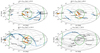 |
Fig. 1. Distribution of orbital poles in Galactic coordinates for the analysed sample of MW satellites. The median orbital poles are shown as open black circles, while the values of 5000 Monte Carlo realisations drawing on measurement uncertainties are shown as coloured dots. The colour scheme follows the division of our sample into on-plane (orange dots), off-plane (blue dots) and uncertain systems (grey dots) detailed in Sect. 2. |
Positions, velocities, and orbital poles of the MW satellites considered in this work.
We define as ‘on-plane’ those systems with a fVPOS > 0.95 (i.e. with a large fraction of their orbital poles distribution aligned with the VPOS normal vector). This definition includes both co- and counter-orbiting systems along the VPOS. The ‘off-plane’ systems have fVPOS < 0.05, while the remaining galaxies have intermediate fVPOS values, making their association with the VPOS uncertain. This is mainly due to the highly uncertain orbital pole directions because of the relatively high uncertainties in proper motion (see Fig. 1).
The distribution of fVPOS values, shown in Fig. 2 (left panel), is bi-modal with 16 systems resulting on-plane and 17 off-plane. We note that satellites located outside the VPOS area only on the basis of their spatial position (i.e. having  ) are assigned to the off-plane sample independently of their proper motion accuracy. These are: Hercules, Sagittarius II, Segue 2, Triangulum II, Ursa Major II, and Willman 1. Thus, the off-plane sample is by definition more complete, since it can include systems having less constrained proper motions and thus poorly determined orbital properties. We also note that the orbital poles of the on-plane sample are confined on a much smaller area (∼20% of the sky) with respect to the off-plane sample, and yet both contain a similar number of satellites. This highlights the overdensity of the VPOS-aligned objects; if they were distributed uniformly, there would be four times more in the non-VPOS area.
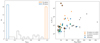 |
Fig. 2. Sub-sample selection. Left: distribution of the fraction fVPOS of Monte Carlo realisation for the orbital poles of our systems that are found within the VPOS area (i.e. within θVPOS = 36.87° from the orbital pole of the VPOS normal). Right: distribution of the V-band luminosity values for our systems as a function of their Galactocentric distance. In both panels, the on-plane systems are plotted in orange, the off-plane ones in blue, while systems with intermediate fVPOS are marked in grey. In the right panel, they are plotted using filled triangles (pointing up or down depending on whether a system is co- or counter-orbiting within the VPOS), circles and squares, respectively. In addition, black circles indicate the MCs and likely associated satellites, while green circles mark those systems that are in the off-plane sample independently of their proper motions. |
It is also instructive to consider the distribution of luminosity values of our systems as a function of their Galactocentric distances, as shown in Fig. 2 (right panel). This figure is complementary to the distribution of orbital poles shown in Fig. 1. We can see that systems with intermediate values of fVPOS (and therefore labelled as uncertain) are either low-luminosity or distant dwarfs, which has an impact on their proper motion determination (their associated errors are on average a factor of 10 larger than those of the on- and off-plane sub-samples), and thus on their orbital pole distributions. On- and off-plane systems have proper motion errors that translate into comparable average tangential velocity errors ∼30 km s−1, with only Columba I and Reticulum III (both among the off-planes) having large errors > 70 km s−1. These two systems are faint satellites whose exclusion from the off-plane sample would not impact our results.
We further note that there are systems such as Carina II (and marginally Draco II, Segue 1, but also Leo I and II at greater distances) which, based on their  , are located just outside the VPOS area (see again Fig. 1). In particular, Carina II is with high probability a former satellite of the LMC (Battaglia et al. 2022), which instead is safely on the VPOS. Indeed, the LMC has probably brought in several dwarf satellites in its fall into the MW potential (we consider here the most likely associated systems listed in Battaglia et al. 2022, but see also Correa Magnus & Vasiliev 2022). As they might follow similar orbits, they would not be an independent sample and could increase the presence of dwarf galaxies on the VPOS (Pawlowski et al. 2022). Therefore, in the following section we also take into account the contribution of the LMC satellite system.
3. Comparison of the physical properties
In Fig. 3 we compare the photometric (i.e. visual luminosity LV; semi-major axis half-light radius Re; weighted-average metallicity ⟨[Fe/H]⟩) and dynamical (i.e. velocity dispersion σv; dynamical mass M1/2, as in Wolf et al. 2010) properties of our sample, obtained using values from Table B.1 of Battaglia et al. (2022, and references therein). Plots are made in order to highlight well-known scaling relations between LG dwarf galaxies, such as luminosity-size (Brasseur et al. 2011), luminosity-metallicity (Kirby et al. 2013), luminosity-dynamical mass (Walker et al. 2009; Wolf et al. 2010; McConnachie 2012) and related parameters (i.e. σv and Re).
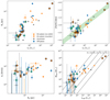 |
Fig. 3. Comparison of the physical properties for our sample of dwarf galaxies. Top left: V-band luminosity LV versus the half-light radius Re. Top right: LV versus the global average metallicity [Fe/H]; the green band is the LV-[Fe/H] relation from Kirby et al. (2013). Bottom left: Re versus the velocity dispersion σv. Bottom right: luminosity Lhalf at the half-light radius versus the calculated dynamical mass Mhalf at the same radius; dashed black lines indicate constant M/L ratios of 1000, 100, 10 and 1, from left to right. In all panels, on- and off-plane systems are represented by orange triangles and blue circles, respectively, while uncertain systems are represented by grey squares. The LMC and its probable satellites are marked with black circles, while green circles mark systems being in the off-plane sample independently of their proper motions. |
We used the Spearman’s rank correlation coefficient ρ to measure the level of correlation between the inspected physical parameters, recovering expectedly high correlation values (i.e. |ρ| ≳ 0.7) when considering the full sample. Restricting the analysis to the on- and off-plane systems, we found instead a marked difference between them in terms of ρ values. As shown in the correlation matrix of Fig. 4, on-plane systems have higher correlation values between the physical parameters than the off-plane ones. In the figure, we also provide ρ values for the orbital parameters described in the next section, for the two MW potentials we considered. We note that in both cases, the upper right part of the correlation matrix shows values for the on-plane sample, while the lower left part is for the off-plane sample.
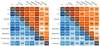 |
Fig. 4. Correlation matrixes showing Spearman’s rank coefficients between the inspected physical (luminosity, half-light radius, global average metallicity, velocity dispersion) and orbital parameters (pericentre, apocentre, eccentricity, time since the last pericentric passage) in the case of a low (left panel) and high (right panel) mass MW potential. In both cases, the upper right part corresponds to values for the on-plane sample, while the lower left part is for the off-plane sample; orange and blue shades correspond to the numerical values shown, with darker shades corresponding to a stronger correlation. |
Considering that for the full sample the relations between the inspected physical parameters are mostly linear, the differences observed when dividing into on- and off-plane systems are mainly due to the lack of luminous systems (i.e. with LV ≳ 105 L⊙) among the off-plane sample (2 vs. 8, respectively). This is best shown in Fig. 5, where the cumulative luminosity distributions of the two sub-samples are compared. We have used the absolute magnitude MV in the figure to highlight the observed difference at the bright-end of their distributions. The observed luminosity gap between the two samples is for MV ∼ −8.
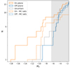 |
Fig. 5. Cumulative luminosity distribution of the satellites on-plane (orange solid line) compared to those off-plane (blue solid line); the distribution of the uncertain systems is reported too for comparison (grey solid line); dashed lines show the same comparison but removing the MC system. The grey band indicates the search completeness on the SDSS footprint (Koposov et al. 2008; Walsh et al. 2009; Simon 2018). |
Before examining the significance of this result, we first note that systems being in the off-plane sample independently of their proper motions (because they have  ) do not contribute to the observed luminosity gap, since they all have a luminosity LV < 105 L⊙ (i.e. MV > −6, see Fig. 2 right). We also note that on-plane systems are brighter than the off-plane ones even as a function of the Galactocentric distance (see again Fig. 2 right).
We compared the luminosity distribution of the on- and off-plane samples using two-sided Kolmogorov-Smirnov (KS) and Anderson-Darling (AD) statistical tests, recovering p-values of 0.15 and 0.05, respectively. Similar results are also obtained for the Re, ⟨[Fe/H]⟩, and σv distributions due to the existing scaling relations, as shown in Table 3, where we also report the average distribution values of the inspected parameters. Therefore, we cannot reject with high formal significance the hypothesis that the two samples come from the same parent distribution. Even though the observed luminosity gap is highly suggestive of this, we thus cannot firmly establish it, mostly due to the relatively low total number of dwarf galaxies involved.
Average distribution values and statistical test results.
The above results are linked to two main sources of uncertainty that could influence them. These are the incompleteness of the MW luminosity function, and the inclusion of satellites with an uncertain orbital pole in one of the two samples.
Regarding the first point, we observe that the largest difference between the inspected distributions is in a luminosity range where the MW luminosity function is considered to be mostly complete, while yet-to-be-discovered satellites are expected to be ultra-faint dwarfs with MV ≳ −7 (Simon 2018, but also Koposov et al. 2008; Walsh et al. 2009). It is true, however, that the discovery of the Antlia II and Crater II dSphs (Torrealba et al. 2016, 2019), suggests that even at the bright-end of the MW luminosity function there might still be some systems missing. In fact, the inclusion of a number ≥1 of Antlia II-like systems with MV = −9 in the off-plane (on-plane) sample would significantly reduce (increase) the statistical significance of the observed luminosity gap. A similar argument would also apply if the Sagittarius dSph (MV = −13.5) were included in the off-plane sample (see e.g. Pawlowski & Kroupa 2020, for details on its orbital properties). We recall that we have excluded this galaxy from our analysis because its observed properties are strongly influenced by the ongoing tidal disruption caused by the MW.
Regarding the second point, there are a number of bright systems (i.e. MV ≤ −7) with an uncertain orbital pole determination based on Gaia proper motions, due to their large Galactocentric distances: Leo I, Leo II, Canes Venatici I, and Eridanus II. Canes Venatici I, despite the uncertainties, has its median orbital pole value almost perfectly aligned with the VPOS, while the median values of Leo I and II are close to the θinVPOS area (see Fig. 1). For the latter two systems, studies have shown that their orbital poles are much better aligned with the VPOS combining Gaia’s astrometric measurements with those of the Hubble Space Telescope, in order to reduce the uncertainty on proper motions (Pawlowski & Kroupa 2020; Casetti-Dinescu et al. 2022). Adopting these additional proper motion measurements thus results in including these three galaxies in the on-plane sample, while Eridanus II is added to the off-plane sample. Even including Sagittarius in the off-plane sample then not only maintains the large gap at the bright-end between the luminosity distributions of the on- and off-plane samples, but in fact does so with high statistical significance (KS and AD tests returning p-values < 0.05).
The above points show that it is crucial not only to improve the proper motions of distant bright systems to firmly establish their association with the VPOS, but also to have a uniform coverage of the sky to find potentially missing bright systems. A further concern indeed is that the footprint of current surveys may influence the number of satellites that end up on the VPOS. Pawlowski (2016), analysing the footprint of the Sloan Digital Sky Survey (SDSS), ruled out this possibility by showing that the SDSS satellites found then increased the significance of the VPOS (see also Metz et al. 2009).
Considering the contribution of the MC system, the LMC in its infall into the MW potential has probably brought in, together with the SMC, a number of faint satellites (we consider here those identified in Battaglia et al. 2022) and marked in Table 2, (but see also e.g. Patel et al. 2020). The LMC associated systems have orbital poles mostly aligned with the VPOS (except for Carina II, which however is just outside the θinVPOS area; see Fig. 1). By removing the LMC and associated systems, the observed gap between the luminosity distributions of the on- and off-plane samples is still present at MV ∼ −8, as shown in Fig. 5, although less severe (six counts compared to the previous eight). We note that in this case we are taking a conservative approach since the LMC, being an independent object, could be left in the count of on-plane systems.
4. Comparison of orbital dynamics
The analysis of the orbital properties of our sample depends necessarily on the assumed MW potential for calculating the orbital parameters. Therefore, we first inspect the velocity vector of our systems, which is independent of such assumptions, focusing on their radial and tangential velocity values. Then, we continue inspecting the orbital parameters (i.e. pericentre, apocentre, eccentricity, period, time since the last pericentric passage, together with other parameters we derived from them) made publicly available by Battaglia et al. (2022), obtained assuming two different MW potentials. We note that from Battaglia et al. (2022) we have only used tabulated values of the orbital parameters, whereas we explicitly state when we performed our orbital integration.
4.1. Kinematic properties
Our on-plane and off-plane samples were selected on the basis of the orbital poles of the satellite galaxies. The categorisation thus depends only on the accuracy of their tangential velocity direction (since the orbital pole is the normalised cross product of the Galactocentric position and velocity vector) and is therefore independent of the radial component and the absolute value of the tangential component of the velocity vector. We check here whether the on-plane and off-plane samples differ in these velocity components with respect to the MW.
In the left panel of Fig. 6, we show the Galactocentric radial velocity component Vrad of our systems1, which mostly depends on their line-of-sight velocity, compared to the median angular difference between their orbital poles and the VPOS normal, θVPOS. This reveals a striking feature: the majority of the co-orbiting on-plane systems are currently approaching the MW (Vrad < 0), while both counter-orbiting on-plane systems are receding from it. Only four of the 14 co-orbiting satellites do not contribute to this pattern: two have clearly receding velocities (i.e. Carina III and the LMC), while the other two have almost zero radial velocity (i.e. Carina and the SMC). This is in contrast to the radial velocity distribution of the off-plane (as well as the uncertain) systems, which distribute evenly around Vrad = 0 km s−1. Indeed, the median and median absolute deviation of the co-orbiting systems are −44 km s−1 and 67 km s−1 (−80 km s−1 and 43 km s−1, if we remove the LMC satellites), while for the off-plane systems we have 14 km s−1 and 103 km s−1, respectively. Performing a KS and AD test between the radial velocity distributions of the co-orbiting and off-plane samples, we recover p-values < 0.15, for both tests. The same conclusions are obtained by removing the LMC satellites.
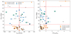 |
Fig. 6. Inspection of the velocity vector components. Left: median angular difference θVPOS between the orbital poles and the VPOS normal for our sample of MW satellites, as a function of their Galactocentric radial velocity Vrad; the red solid line is for reference only, since it helps to identify satellites that are approaching the MW (Vrad[km s−1] < 0) or receding from it (Vrad[km s−1] > 0); the red dashed lines represent the aperture angles around the two opposite poles of the VPOS. Right: θVPOS as a function of the |


We note that the radial velocity pattern is robust and remains unchanged even when we consider the effect of the MW reflex motion caused by the infall of a massive LMC (see e.g. Pawlowski et al. 2022). This pattern implies that almost all co-orbiting VPOS members are currently approaching the MW and thus their respective orbits’ pericenters, while the two counter-orbiting VPOS members are receding and thus had experienced their last pericentre recently. In contrast, the off-plane systems are spread more randomly between approaching or receding, and thus between before or after, their orbits’ nearest pericenter.
Regarding the Galactocentric tangential velocity Vtan properties of MW satellites, it has been reported in the literature that most (∼70 − 80%) of those with measured proper motion show an excess of tangential velocity, meaning that their orbital kinetic energy is dominated by tangential motion (Cautun & Frenk 2017; Riley et al. 2019; Hammer et al. 2021). This seems to be in sharp contrast with the low fraction (∼1.5%) expected from simulations (Cautun & Frenk 2017). We confirm this finding also with the proper motion data used in this work. As shown in the right panel of Fig. 6, we recover a tangential velocity excess for ∼75% of the satellites (i.e. having  ), both considering each sub-sample or taking them as a whole. Furthermore, we do not find particular differences between the on- and off-plane samples in this regard, although the LMC satellites are more tangentially biased than the other on-plane systems. It can be argued that the observed tangential velocity can be a biased estimator of the true value, but as already noted in Battaglia et al. (2022), such biases are minimised for measurement uncertainties < 70 km s−1. As reported in Sect. 2, our on- and off-plane systems are safely within this limit.
4.2. Orbital properties
We inspect now the orbital parameters (i.e. pericentre, apocentre, eccentricity, period, and time since the last pericentric passage) made publicly available by Battaglia et al. (2022), obtained assuming either a low-mass (Mvir = 8.8 × 10¹¹ M⊙ within rvir = 251 kpc) or a high-mass potential (Mvir = 1.6 × 10¹² M⊙ within rvir = 307 kpc) for an isolated MW. The former is a triaxial potential published originally in Vasiliev et al. (2021), while the latter is a scaled and more massive version of the MWPotential2014 from Bovy (2015). Such potentials bracket the range of likely MW masses, which distribute around Mvir ∼ 1012 M⊙ (e.g. Wang et al. 2020, and references therein). We note that for some systems only the lower limits of their orbital parameters are available, since they do not reach their apocentre during the orbital integration period2. We also warn that these orbital parameters are not free of biases, particularly with regard to tangential velocity, but as already mentioned, we are within safe limits. For more details on the MW potentials and how the orbital parameters were derived, we refer to Battaglia et al. (2022).
Comparison of the orbital parameter distributions between on- and off-plane samples shows no significant differences using the KS and AD statistical tests, for both MW potentials (see again Table 3). Similarly, analysing the level of correlation between the orbital parameters, we found low values (i.e. |ρ| ≤ 0.5) for both samples considering the high-mass potential case, while we found stronger values among some parameters in the low-mass potential case (see again the correlation matrix in Fig. 4, but also Figs. A.2 and A.3). We caution, however, that in the latter case stronger |ρ| values may arise because fewer targets have a complete orbital solution, which may lead to possible spurious correlations between parameters.
An additional aspect we examined is related to the excess of MW satellites found near their orbital pericentre, first reported using the second data release of Gaia (see Fritz et al. 2018; Simon 2018). This is a potential problem because, as MW satellites are on eccentric orbits, one would expect to find them close to their apocentre, where they spend more time. Pawlowski (2021) confirmed the significance of the pericentre excess by also analysing the orbital parameters of Battaglia et al. (2022), finding that such an effect is more prominent when the low-mass MW potential is assumed, in agreement with previous results (e.g. Li et al. 2021, but see also Correa Magnus & Vasiliev 2022). This problem may be related to the tangential velocity excess described in the previous section, since the radial velocity is minimal around the pericentre. As in that case, we checked for possible differences between the on-plane and off-plane samples in the distribution of fperi, the fractional distance in time of a satellites to be found between pericentre (fperi = 0) and apocentre (fperi = 1), finding none significant (see further details in Appendix A).
The preferred negative radial velocities of the co-orbiting on-plane systems have already indicated a clear preference of this sample of satellites to move towards their pericentre. We now investigate this in more detail using the full orbit integration, taking into account whether a satellite is moving towards or away from the pericentre and in what orbital phase it is in. Again, we find that the co-orbiting on-plane systems preferentially approach their pericentre, but they also show a remarkable pattern in their time since pericentre. This is illustrated in the top panels of Fig. 7, where we inspected tperi, the time to the next (tperi > 0) or since the last (tperi < 0) pericentric passage as a function of P, the satellites’ orbital period. In both figures, the solid red line indicates that a satellite is at its pericentre, the dashed black lines represent when it is at the apocentre (i.e. at ±P/2), while the dotted lines represent when it is halfway between these two points (at ±P/4). Therefore, a satellite leaving its apocentre, passing through its pericentre and then returning to the apocentre, evolves on the diagram going from positive to negative tperi values. If there is a group of satellites with different P leaving their apocentre at the same time, they move towards their pericentre parallel to the upper dashed line shown in the figure. This seems to be the case for the on-plane systems: the majority of the co-orbiting satellites are moving towards their pericentres after having left their apocentres ∼1 Gyr ago, while the counter-orbiting systems have just passed their pericentres.
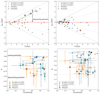 |
Fig. 7. Inspection of the orbital parameters. Top: time to the next or since the last pericentric passage, tperi, as a function of the satellites’ orbital period, P, both in units of Gyr; the red solid line at tperi = 0 indicate when satellites are at pericentre, the thin dashed lines indicate the apocentre limits, while the dotted lines mark the half-orbit; the thick dashed line, shown for illustrative purposes, is parallel to the upper apocentre line, shifted by ∼1 Gyr. Bottom: satellite orbital phases, ϕ, as a function of the orbital eccentricity; thin dotted lines represent the limits when a satellite has just left its pericentre (ϕ close to 0), or is approaching it (ϕ close to −1). Panels on the left show values obtained with the low-mass MW potential, while those on the right with the high-mass MW potential. In all panels, symbols and colours are as described in Fig. 3. |
Our result holds true for both Galactic potentials adopted, although it is more striking for the low-mass potential, which is more realistic in light of recent MW mass estimates (e.g. Bird et al. 2022, and references therein). The systems that deviate most from this pattern are the probable LMC satellites, which however have more uncertain orbital parameters and should not be considered as independent satellites. Therefore, if we exclude them, we are left with only one system that does not follow the pattern in either case, the Carina dSph. We note that this system has a radial velocity with respect to the MW that is consistent with zero (see Fig. 6), so its orbital properties depend strongly on its tangential motion and the assumed MW potential and it can either be close to peri- or apocenter, or on a circular orbit. It follows that Carina has an uncertain apocentre and eccentricity in the case of the low-mass potential, while for the high-mass potential its orbit is mostly circular, which leads to large uncertainties in the orbital period in this case as well. In both cases, its position within the errors is consistent with approaching the pericentre and can therefore be associated with the rest of the co-orbiting systems.
A complementary way to highlight the coordinated motion of the on-plane systems is by inspecting the satellites’ orbital phase ϕ (i.e. the ratio between the time since the last pericentric passage and the orbital period). In our definition, a satellite with ϕ close to 0 has just left its pericentre, whereas if ϕ is close to −1 it is approaching the pericentre. Similarly to the previous case, we find that almost all systems co-orbiting (counter-orbiting) within the plane have comparable ϕ values, within errors, and move towards (away from) their pericenters for both potentials, as shown in the bottom panels of Fig. 7, where we plot ϕ values as a function of orbital eccentricity. Such a result is again more pronounced in the case of the low-mass potential, where the ϕ distribution of the on-plane systems differs significantly from that of the off-plane systems (see Table 3). Performing KS and AD tests to assess that the ϕ distribution of on-plane satellites is not drawn from a uniform distribution yields significant p-values < 0.05, considering only co-orbiting satellites. We can thus reject the hypothesis that the co-orbiting satellites are found in random orbital phases. This result is valid for both potentials, whereas the inclusion of counter-orbiting systems would cause it to lose significance only in the case of the less realistic high-mass potential. This result is also not dominated by the LMC satellites (for which we can be confident that their orbital phase is not random but linked to that of the LMC) and is still present for co-orbiting on-plane satellites not linked to the LMC (leading to p-values of ∼0.04 and ∼0.06 for the low and high mass potentials, respectively). We also note that the co-orbiting systems share similar eccentricities values, with a small scatter. High p-values are instead obtained by analysing whether the ϕ distribution of the off-plane systems is drawn from a uniform distribution, indicating that they are consistent with random orbital phases.
Although the large errors associated with ϕ, especially for the low-mass potential case (see Fig. 7 again), limit our interpretation of the orbital motion of the on-plane systems, the radial velocity of the co-(counter)orbiting systems alone already clearly indicates that they are approaching (moving away from) the MW. The expected phase mixing of the on-plane systems approaching the MW depends on their orbital periods and that the relevant timeline to wash out the observed coherence is of the order of ∼1.5 Gyr (i.e. half of the difference between the minimum and maximum of their P values). Therefore, the observed ϕ distribution mixes relatively quickly. If we evolve the positions of the satellites on the tperi − P plane, we observe that the current configuration of the on-plane systems does not repeat itself for at least a Hubble time. This could indicate that the on-plane systems have only recently arrived in the MW potential, possibly as a group of dwarf galaxies, although there is also the possibility of a chance event. In the next section we consider the possible role of the LMC.
4.3. The role of the LMC
Several lines of evidence have been presented in the literature in support of a massive LMC (i.e. between 1 − 2 × 10¹¹ M⊙) that has just passed its pericentre, probably for the first time (see Vasiliev 2023, for a review). Such a massive halo can significantly affect the orbits of MW satellites (Patel et al. 2020; Battaglia et al. 2022; Correa Magnus & Vasiliev 2022; Makarov et al. 2023), but it can also cause changes in the MW itself, such as the reflex motion of the MW centre caused relative to its more extended dark halo by the gravitational pull of the LMC (Garavito-Camargo et al. 2019, 2021; Petersen & Peñarrubia 2020, 2021; Vasiliev et al. 2021). In particular, Garavito-Camargo et al. (2021) showed the ability of the LMC to produce an excess of orbital poles of dark matter halo particles towards its own pole direction, although Pawlowski et al. (2022) showed that this might be insufficient to explain the presence of MW satellites co-orbiting along the VPOS. Here we rather discuss the impact of the LMC on the orbital analysis results shown above.
In this regard, we have further investigated the orbital properties of MW satellites by considering the low-mass MW potential perturbed by a 1.5 × 10¹¹ M⊙ LMC, first introduced in Vasiliev et al. (2021) and then used in Battaglia et al. (2022) to study the effects of such a massive LMC on the orbital properties of MW satellites. They found that, as far as the VPOS satellites are concerned, especially the bright ones, Sculptor would be on its first infall, while Carina and Fornax would have a fraction (25% and 4%, respectively) of their Monte Carlo orbit realisation linked to the LMC, the former possibly being a past satellite. On the other hand, the former LMC satellites would not yet be in a closed orbit (or have reached their pericentre). These results depend on the assumed masses of the MW and LMC, but they already underline that the effect of the LMC on the orbits of other MW satellites may not have been negligible (see also Correa Magnus & Vasiliev 2022; Makarov et al. 2023).
In our case, we checked the possible influence of the LMC in comparison with the results in Sect. 4. We used the code Agama (Vasiliev 2019) to integrate the orbits of our sample of satellites assuming the aforementioned perturbed potential of Vasiliev et al. (2021). This is a time-dependent potential of the MW that takes into account the trajectory of a massive LMC, which entered the dark matter halo of the MW about 1.6 Gyr ago, and the acceleration induced by the reflex motion of the MW. We integrated the orbits backwards for 5 Gyr from 100 Monte Carlo realisations of the position and velocity of our systems generated from their present values (see Table 2). The orbital parameters (time since last pericentre, period, eccentricity and phase) were calculated for each realisation, from whose distributions we derived their median and, as uncertainties, the 16th and 84th quantiles. We note that for the LMC and its satellites, which in this case are at their first infall, orbital parameters have not been recovered, a part for tperi when available.
As shown in the top panel of Fig. 8, we find that the co-orbiting on-plane systems are still approaching their pericenters (again excluding Carina), but with changes in their tperi and P, here to smaller values compared to the low-mass potential case. This is expected due to the higher total mass of the combined MW and LMC. Looking at the bottom panel, we again see that the co-orbiting on-plane systems have ϕ < −0.5, meaning that they are approaching the pericentre, but on less eccentric orbits, as is also the case for the other satellites. The associated errors are, however, larger since the influence of the LMC makes the determination of orbital parameters more uncertain.
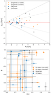 |
Fig. 8. As in Fig. 7, but considering results obtained with a MW potential perturbed by a massive LMC (see details in Sect. 4.3), in the top panel is shown the time to the next or since the last pericentric passage, tperi, versus the satellites’ orbital period, P, while in the bottom panel the satellites’ orbital phases, ϕ, versus the orbital eccentricity. We note that while some systems have a measured tperi, they may not have a closed orbit and therefore have P = 0 (such as the LMC and its satellites). |
Despite the significant influence of the LMC and the uncertainties it introduces, we confirm our previous finding that co-orbiting on-plane systems approach the pericentre, although it is uncertain whether they do so in a coordinated manner. It therefore appears to be a signal independent of the presence of the LMC and thus not caused by it.
4.4. Energy and angular momentum properties
Before discussing the implications of our results on possible scenarios for the formation of the VPOS, we first examine the properties of our satellite sample in terms of specific energy E and angular momentum L at the present time. As already noted by Hammer et al. (2023), satellites associated with the VPOS have minimal specific energy E values for a given angular momentum L, closely following the relation for circular motion on the E − L plane. We confirm this result, as shown in the left panel of Fig. 9, where we see that the on-plane systems generally tend to have the lowest E for a given L2, in contrast to the other satellites which show a larger scatter. In the right panel, we instead plot E versus the specific angular momentum in the Cartesian x-direction of a Galactocentric reference frame, Lx, and again find that the on-plane systems tend to have the lowest E for a given Lx value3. In both panels we only show the E values obtained for the low-mass potential, but similar conclusions are drawn for the high-mass potential, and also for the LMC perturbed potential considered in the previous section. These results seem to indicate that the VPOS has a cold dynamics, rather than being formed by satellites on their first arrival. A comparison can be made with the LMC system (which arrived < 2 Gyr ago), whose satellites (including the LMC) have on average higher E for a given L. In the next section we discuss the implications for the longevity of the VPOS in the light of these results in combination with the previous ones.
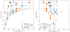 |
Fig. 9. Inspection of the energy and angular momentum values. Left: total specific energy E (in units of 104 km s−1) versus the square of the specific angular momentum L (in units of 109 kpc2 km2 s−2) at the present time; dotted line represents the relation for a particle of negligible mass on a circular orbit. Right: E against the specific angular momentum in the Cartesian x-direction of a Galactocentric reference frame, Lx (in units of 103 kpc km s−1); the red solid line at Lx = 0 is for reference only. In both panels, symbols and colours as in Fig. 3; error bars for the uncertain systems, which are large, are not shown for clarity. |
5. Discussion
Our comparison of the satellite galaxies associated with the VPOS and those that are not has revealed several distinct differences in their properties: the known on-plane satellite galaxies tend to be more luminous; they show a strong pattern in their orbital phases, with the majority of the co-orbiting satellites currently approaching their pericenters, while the two counter-orbiting satellites have both recently passed their pericenters. In addition, the on-plane satellites not associated with the LMC tend to have the lowest orbital energies for a given angular momentum value. We shall discuss then what are the implications for the longevity of the VPOS in light of our results.
The possibility that the LMC system is on its first pericentric passage (Vasiliev 2023, and references therein) and the fact that most of its components are part of the on-plane sample seems to indicate that the VPOS is a dynamic structure that could be currently forming. The question is therefore how long the other on-plane systems have been part of the VPOS and whether they have been associated with the LMC in the past. We can see two possible interpretations: (i) the on-plane systems not currently associated with the LMC are long-time satellites of the MW, having completed several pericentric passages, and thus they are old members of the VPOS; (ii) they may or may not have previously been associated with the LMC, but have recently entered the MW potential and have completed at most a few pericentric passages.
Assuming that the VPOS is an old structure, as advanced in (i), would imply that the orbital features reported in Sect. 4 are a mere coincidence. We have already seen that it is difficult to interpret the dynamic properties and phase alignment of the on-plane systems in this way, but it is also true that these aspects have not been yet investigated in the context of cosmological simulations. In fact, such comparisons have focused rather on the spatial flattening and clustering of the orbital poles of the simulated systems. We leave this topic for a future study, while we focus here on further investigating point (ii), which interprets the observed orbital features as a significant property of the VPOS from which clues about its origin can be deduced (which a chance alignment does not allow).
The interpretation that the VPOS may be a rather young structure, as proposed in (ii), mainly concerns three aspects, all related to the late accretion of satellite systems: (a) VPOS members are tidal dwarf galaxies (TDGs) formed after a major merger or close interaction between the MW and another galaxy; (b) the VPOS may be the result of a late merger experienced by the MW, but in this case its components are the former satellites stripped from the merged galaxy; (c) VPOS members were part of a bound group of dwarf galaxies that was tidally stripped by the MW and has not yet had time to fully phase mix.
The proposed scenarios underline the complexity of understanding the origin of the VPOS. As each of them deserves an in-depth study that would go beyond the scope of this article, we limit ourselves in the following sections to exploring their implications given our findings.
5.1. Do on-plane systems have a tidal origin?
The possibility that the VPOS is populated by TDGs was one of the first proposals put forward on its origin (Lynden-Bell 1976; Kunkel 1979). Indeed, TDGs are second-generation galaxies that form in a common tidal tail from material recycled from a previous collision, thus sharing its orbital plane orientation. Being dark-matter-free systems with a high gas content at the time of formation, TDGs are also more likely to experience the effects of ram-pressure stripping and tidal disruption during their orbit around the host galaxy than dark-matter-dominated systems (Klessen & Kroupa 1998, Yang et al. 2014, but see also Ploeckinger et al. 2015). Therefore, if we take into account that TDGs could disperse after approaching the MW, we could assume that the ones currently observed are on a first pericentric passage and interpret this as consistent with the strongly skewed orbital phase distribution we found, where the majority of co-orbiting VPOS members are currently located ahead of their respective pericenters.
Interestingly, the peculiar observed orbital phase distribution is reminiscent of a proposal by Pawlowski et al. (2011) to explain the presence of counter-orbiting satellite galaxies aligned with the VPOS. In this model, tidal debris from a past galaxy collision accumulates on orbits around the MW. As the tidal debris tail, in which TDGs are formed, passes over the centre of the MW, its orbital direction changes and the later accreted TDGs move in the opposite orbital direction to the earlier accreted ones. This is consistent with one orbital direction (the two counter-orbiting VPOS members) having recently passed their pericenters and thus being further along their orbits than the co-orbiting satellite galaxies, which are still approaching their pericenters. This would imply that the TDG members of the VPOS only arrived in the last few Gyrs around the MW (as envisaged in e.g. Fouquet et al. 2012).
Based on the analysis of Gaia data, Hammer et al. (2021) suggested that VPOS systems may have entered the MW potential < 3 Gyr ago as gas-rich dwarf galaxies that lost their gaseous content due to ram pressure stripping, which also caused a deceleration along the radial direction of their orbits. This mechanism is most efficient for luminous dwarfs, which in fact dominate the VPOS population (see Sect. 3), but also assumes that they are TDGs formed in a past merger event between the MW and Andromeda (see e.g. Yang et al. 2014).
In the scenario in which the VPOS systems are late-arriving TDGs, we would expect them to be different from other MW satellites, which are instead dark-matter dominated dwarf galaxies that have followed different formation and evolutionary paths. In particular, TDGs should be more metal-rich than the general population of dwarf galaxies because they would have formed from the recycled enriched material released by the merging parent galaxies.
In Fig. 10, we show the difference between the observed weighted-average ⟨[Fe/H]⟩ and the expected values from the Kirby et al. (2013) relation for the selected sub-samples. The on-plane satellites show a median offset of −0.06 dex, while the off-planes of 0.12 dex (0.06 dex for the uncertain sample). The ∼0.2 dex difference between the on- and off-plane samples is mainly driven by the faint satellites with LV < 103 L⊙, which tend to no longer follow the observed luminosity-metallicity relation, but rather a flat trend with LV characterised by significant scatter (also Simon 2018). If we limit the analysis to LV > 103 L⊙, we find that the on- and off-plane samples show similar offsets of −0.06 dex and −0.02 dex, respectively, which are well within the rms scatter of the Kirby et al. relation. We note that the probable LMC satellites tend to be more metal-poor than the Kirby et al. relation, with a median offset of ∼ − 0.1 dex (excluding Carina III, which is at the low-luminosity end, due to its uncertain metallicity value obtained from an isochrone fitting, Torrealba et al. 2018). It is difficult, however, to establish the significance of such result, considering that the metallicity values come from heterogeneous sources (see references within Battaglia et al. 2022). Therefore, the faint end of the luminosity-metallicity relation deserves further investigation, since it is still unclear what are the causes of the large scatter observed, whether it is mainly due to observational errors or an actual physical cause, such as tidal and ram-pressure stripping (see e.g. discussion in Simon 2018).
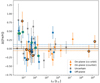 |
Fig. 10. Difference between the observed weighted-average ⟨[Fe/H]⟩ of our galaxies and the expected values at their luminosity obtained from the Kirby et al. (2013) relation; symbols and colours as in Fig. 3. Error bars obtained adding in quadrature the errors on ⟨[Fe/H]⟩ and the rms = 0.17 dex of the Kirby et al. relation for the MW satellites. Dashed lines are the median offsets of each sub-sample. |
On a broader perspective, our results constitutes a tight constraint on the hypothesis that the on-plane systems might be TDGs, while the off-plane systems are not. In fact, for them to follow the observed luminosity-metallicity relation, they should have formed from low-metallicity material ejected during an early merger event (z ≳ 1) between the MW and another galaxy (see Recchi et al. 2015, but also Ploeckinger et al. 2018 and Dumont & Martel 2021), probably Andromeda (e.g. Hammer et al. 2010, 2013; Yang et al. 2014). The TDGs thus formed should then have evolved for several Gyrs as regular dwarf galaxies, maintaining similar size and dynamical mass to the off-plane systems for several orders of magnitude (although they are expected to follow a different mass-size relation, e.g. Haslbauer et al. 2019). We recall, however, that TDGs are more likely to be significantly affected by tidal and ram-pressure stripping. Therefore, if they were long-lived satellites of the MW, it would be difficult to understand how they could have survived for so long and exhibit properties similar to those of the off-plane systems.
Our conclusions are in agreement with those reached on a similar basis by Collins et al. (2015), who argued against a tidal origin for the dwarf galaxies on the great plane of Andromeda. We finally note that the scenario in which VPOS systems are TDGs has other alternatives that abandon the dark matter paradigm in favour of models based on modified Newtonian dynamics (MOND; see Banik et al. 2022 for an extensive introduction on TDGs in a MOND scenario and an application to the MW-Andromeda case), although there are limitations here too (see Pawlowski 2018, for a review).
5.2. A link between the VPOS and the MW’s merger history?
We introduced the possibility that the VPOS could be the result of a merger event in which a galaxy brings its own satellite population when it merges with the MW. Smith et al. (2016) showed that, under certain conditions, the acquired satellite population can reorganise itself into an extended planar structure with coherent motion around the merger remnant. This raises the question of whether there are specific merger events in the MW’s past that could be responsible for the emergence of the VPOS. One possible association would be with the Gaia-Sausage-Enceladus (GSE), the most recent significant merger identified to date (Belokurov et al. 2018; Haywood et al. 2018; Helmi et al. 2018).
The GSE progenitor is thought to have been accreted about 8 − 11 Gyr ago (Di Matteo et al. 2019; Naidu et al. 2021; Montalbán et al. 2021). Before its infall, the GSE progenitor had a total mass of about ∼1011 M⊙ (Helmi et al. 2018; Mackereth et al. 2019; Kruijssen et al. 2020; Lane et al. 2023), so it is reasonable to assume that it hosted a population of bound satellites, such as the present-day LMC. The exact number and parameters of these satellites are difficult to determine from the available data. However, if we assume that nine VPOS satellites (i.e. excluding the LMC group) were associated with the GSE, the number of ‘genuine’ MW satellites would be about 34 (where some, but fewer than the GSE’s, could have been accreted earlier in other massive accretion events). This gives a GSE-MW merger mass ratio of ≈1 : 4, which is remarkably consistent with the constraints on the GSE merger parameters. In terms of chemical abundance, the average metallicity of the VPOS satellites is lower than the maximum metallicity of the GSE merger debris (≈ − 0.5 dex), so their formation around the GSE progenitor is not precluded.
However, it is not easy to determine whether the VPOS systems were associated with GSE on the basis of their orbital properties. For instance, by analysing stellar debris from GSE, Chandra et al. (2023) found evidence for an associated stream that extends into the MW halo and moves in the plane defined by the Sagittarius stream, but in the opposite direction. We note that the Sagittarius stream defines a plane perpendicular to the VPOS (e.g. Pawlowski & Kroupa 2020), while Hammer et al. (2021) noted the presence of a possible planar structure associated with the Sagittarius dwarf, in which its components are counter-rotating with respect to it. On the other hand, the reconstruction of the infall orbit of the GSE progenitor is hindered by various dynamical effects (Vasiliev et al. 2022; Dillamore et al. 2022) that together with the growth of the MW potential (Panithanpaisal et al. 2021; Khoperskov et al. 2023) affect stellar debris differently from the globular clusters and satellite galaxies associated with them (Pagnini et al. 2023).
Nevertheless, we investigated whether the VPOS systems share orbital properties with the globular clusters (GCs) likely to be associated with GSE or other MW streams. We used the compilation of GCs from Massari et al. (2019) and in particular we refer to their classification to distinguish between in situ and accreted GCs (probably associated with GSE/Sequoia, Sagittarius and Helmi streams, but see Pagnini et al. 2023 for possible caveats in the classification). Examining their position on the E − L diagrams shown in Fig. 11, we find no particular orbital features shared between the VPOS systems and any of the considered GC populations. This result should not be surprising, since accreted satellite galaxies are less gravitationally bound to their host (GSE-progenitor in the considered case) than its GC and stars, so they would have undergone stripping earlier and would not necessarily end up sharing the orbital properties of the host galaxy’s stars and GCs. It is also true that by remaining mostly outside the tidal influence of the MW disc, they would be more likely to retain the infall orbital parameters of their progenitor, but whether this applies to the GSE case remains to be demonstrated. Indeed, we would rather expect the orbits of former GSE satellites to be already phase-mixed if their accretion occurred 8 − 11 Gyr ago.
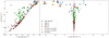 |
Fig. 11. As in Fig. 9, but here including MW globular clusters (GCs) that probably formed in situ (brown hexagons) or were accreted, that is, associated with GSE/Sequoia (green diamonds), Sagittarius (red stars), or Helmi (purple pentagons) streams, according to the compilation of Massari et al. (2019). |
In summary, it is unclear whether the satellites currently comprising the VPOS were initially associated with the GSE progenitor and were stripped away during its infall into the MW. Further efforts are needed to verify the probability of such processes, especially in the context of the orbital phase coherence of VPOS satellites. The analysis of a statistical sample of satellite systems from the IllustrisTNG simulation, however, seems already to indicate that major mergers (i.e. with a mass ratio > 1 : 3) play a negligible role in the formation of correlated planar structures such as the VPOS (Kanehisa et al. 2023).
5.3. Are the on-plane systems part of a group infall?
Group infall is a promising way to explain the origin of a coherent planar structure such as the VPOS (e.g. Lynden-Bell & Lynden-Bell 1995; Li & Helmi 2008; D’Onghia & Lake 2008; Klimentowski et al. 2010). The evidence that the LMC arrived with its own group of satellites (e.g. Patel et al. 2020) also seems to support this hypothesis (see also Samuel et al. 2021). However, it is difficult to determine from orbital integration alone whether the LMC system was part of a single group comprising the other VPOS satellites, or whether they were part of separate groups. For instance, only Carina and Fornax have been suggested to be dynamically associated with the LMC (e.g. Pardy et al. 2020), although this association does not seem to be conclusive (e.g. Patel et al. 2020; Battaglia et al. 2022).
We further note that the accretion of groups of dwarf galaxies is a mechanism already present in cosmological simulations, but the predicted fraction of satellites arriving in groups and the number of dwarf galaxies forming such groups seems insufficient at the moment to explain the formation of a structure such as the VPOS (see Pawlowski 2021, for a review, but also Li & Helmi 2008; Wetzel et al. 2015; Shao et al. 2018). It is true that much remains to be understood about the dependence of the environment in which dwarf galaxy groups form. This is important not only to determine the brightness and compactness of such groups, but also to establish whether they could possibly form a coherent and spatially thin structure such as the VPOS once being accreted. In this context the accretion of (groups of) satellites along cosmic filaments is particularly relevant, a mechanism that provides both a dense environment in which groups can form and a preferential direction for their infall onto a host galaxy (e.g. Libeskind et al. 2011, 2015, but see also Pawlowski et al. 2012b).
The fact that the on-plane systems (excluding the LMC and its satellites) are approaching or moving away from their pericentre showing a strong pattern in their orbital phases can be interpreted as a sign that they have recently arrived in the MW potential together. However, in order to reconcile this scenario with their E − L properties shown in Sect. 4.4, a mechanism is needed to cause them to lose orbital energy. Hammer et al. (2021) proposed ram-pressure stripping as the main energy loss mechanism, capable of reducing radial velocity and circularising orbits. This process, however, is only effective for dark-matter-free galaxies, such as TDGs. We here explore a different approach which instead relies on the dwarfs being heavily dark matter dominated by instead considering a toy model of dynamical friction. Our choice is justified by the fact that the VPOS is dominated by bright satellites on which the effect of dynamical friction should be maximal.
We applied the Chandrasekhar prescription for the induced acceleration by dynamical friction (Chandrasekhar 1943). This formula has provided a good approximation for reproducing the orbital evolution of low-mass objects such as satellite dwarf galaxies (Binney & Tremaine 2008, but also Tremaine 1976; Hashimoto et al. 2003; van der Marel et al. 2012; Patel et al. 2020). One of its terms is the Coulomb logarithm ln(Λ) = ln(bmax/bmin), where bmax and bmin are the maximum and minimum impact factors in an encounter. These terms usually indicate the distance to the centre of the host galaxy, and a deflection radius equal to the half-mass size of the satellite (hence bmax ≫ bmin). However, ln(Λ) can be quite uncertain due to the difficulties in accurately measuring its terms, and while a constant value has usually been assumed, a term varying with distance from the centre of the host galaxy offers better results (Just & Peñarrubia 2005; Petts et al. 2016).
We used the galpy code (Bovy 2015) to integrate the orbits of the luminous dwarfs on the VPOS: Carina, Draco, Fornax, Sculptor, Ursa Minor (i.e. part of the classic MW dwarf spheroidals), and the LMC for comparison. We assumed the MWPotential2014 (Mvir = 0.8 × 10¹² M⊙ and rvir = 245 kpc, similar to the low-mass potential) and integrated backwards for 10 Gyr. As total masses for the satellites we assumed four values of MS = (5 × 10⁹; 1010; 5 × 10¹⁰; 1011) M⊙, compatible with abundance matching expectations for such luminous systems (e.g. Bullock & Boylan-Kolchin 2017). We have kept the total mass of the satellites constant during the integration process, since they are expected to have already assembled more than half of their mass at z ∼ 2 (e.g. Sawala et al. 2016; Libeskind et al. 2020; Deason et al. 2022). We also neglect tidal stripping of their dark-matter halos in order to maximise the effects of dynamical friction in our toy model. For the dynamical friction term4, we assumed a varying ln(Λ), with the satellite’s half-mass radius set at 5 kpc (e.g. Iorio et al. 2019). We note that we would reach qualitatively similar conclusions also assuming a constant ln(Λ) = 3 (e.g. Vasiliev et al. 2021).
We found that the effects of dynamical friction begin to significantly affect orbit integration only from MS ≥ 5 × 10¹⁰ M⊙ (see Fig. A.4). This is a rather high mass for classic dwarf spheroidals, which are instead estimated to be currently around MS ∼ 5 × 10⁹ M⊙. In this case we found the effects of dynamical friction to be negligible, in agreement with previous studies investigating the effects of tides on Fornax and Sculptor (Battaglia et al. 2015; Iorio et al. 2019).
The previous exercise did not take into account the evolution of the MW potential, which we included as an additional element. We followed the prescription of Miyoshi & Chiba (2020, in particular their Eq. (2)), but using the halo component of the MWPotential2014 and considering for the time evolution of its concentration parameter c(Mvir, z) the relation provided by Dutton & Macciò (2014). We integrated the orbits in steps of 10 Myr, assuming two values for the total mass of the individual satellites: MS = 5 × 10⁹ M⊙ and MS = 5 × 10¹⁰ M⊙ (chosen as a representative total mass for a dwarf spheroidal and as the minimum mass at which we saw the orbits start to be significantly affected).
As shown in Fig. 12, the inclusion of an evolving potential does indeed have a significant impact on orbital recovery. At the assumed high-mass limit, three satellites cross the MW virial radius as early as 6 Gyr ago, while the other three at much recent times (< 2 Gyr ago), none making more than a single pericentric passage. For the more plausible low-mass limit, the majority of satellites cross the virial radius around 8 Gyr ago, but in this case the satellites make as many as two pericentric passages. This is in contrast to the previous case with a static MW potential, where satellites at this mass stayed on average within the MW virial radius during the integration period (see Figs. A.5 and A.6).
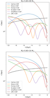 |
Fig. 12. Orbital evolution of the bright dwarfs of the VPOS integrated backwards in time for 10 Gyr, assuming an evolving MW potential and taking into account the effects of dynamical friction, with the satellites assumed to have an individual total mass of MS = 5 × 10⁹ M⊙ (top panel) or MS = 5 × 10¹⁰ M⊙ (bottom panel). The black solid line represents the evolution of the virial radius of the MW. |
Although our approach of estimating infall times by orbit integration is simplistic, due to the inherent difficulty of knowing the MW potential and its evolution over time accurately (e.g. D’Souza & Bell 2022; Santistevan et al. 2024), it is nevertheless helpful to draw some qualitative conclusions. The first is that in order for the classic dwarf spheroidals to have a late arrival into the MW potential, we would have to assume too high masses for them. Even allowing for an evolving MW potential, at the low-mass limit they still tend to make some pericentric passages over several Gyr. Therefore, if we consider them as independent systems, it is difficult to see how they can now exhibit an orbital coherence such as that described in Sect. 4, considering that orbital phases tend to mix in a few Gyr. It may also be that such systems were significantly more massive at the time of first infall and were severely tidally stripped by the MW, although their current stellar populations do not appear to show significant signs of this (e.g. Battaglia et al. 2022).
On the other hand, a natural hypothesis would be to consider the satellites in question having been part of a group of dwarf galaxies. We have already seen that a late arrival in the MW potential requires masses (i.e. MS ≥ 5 × 10¹⁰ M⊙) that are too high for individual systems (excluding the LMC), but compatible with that of a group comprising the classic dwarf spheroidals considered here. We verified that in this mass range it is possible that they shared a similar spatial position when they were crossing the MW virial radius, ∼6 Gyr ago, but mainly because the uncertainties became too large at this point in time (see Fig. A.7). Therefore, to test the hypothesis of group infall it would be necessary to move forwards from simple orbital integration and set up a dedicated study involving cosmological simulations, which we reserve for future work.
If group accretion were the case, further aspects to consider would be the formation environment of this group of dwarf galaxies (e.g. Libeskind et al. 2011) and the subsequent tidal stripping by the MW after an initial pericentric passage that would have contributed to its disruption (e.g. Li & Helmi 2008). More recently, Vasiliev (2024), exploring the implications that the LMC may be on its second pericentric passage around the MW, have speculated on the origin of the VPOS and the possibility that the present on-plane systems may have formed together with the LMC a primordial group from which the luminous satellites were stripped off in a first passage occurred some 6 Gyr ago. As noted by the author, the scenario proposed by Pawlowski et al. (2011) and reported above would still be valid in this context. Instead of accreted TDGs, we would have a group of dwarf galaxies tidally stripped by the MW, eventually forming the VPOS.
The possibility that the VPOS is the result of a single group accretion is intriguing, but as already noted by Vasiliev (2024) is a complex matter that deserve further investigation, in particular to establish whether or not the LMC and its satellites belonged to such a group. The accretion of groups of dwarf galaxies on MW-like hosts has been poorly studied in the literature (see Pawlowski 2021), in particular when related to the formation of plane of satellites. Our results place emphasis on this particular mechanism that deserves further exploration.
6. Conclusions
We compared the observed properties of a sample of 50 satellite galaxies of the MW, looking for differences between systems on and off the VPOS. In particular, we compared their physical and orbital properties.
The comparison of the physical properties using different parameters (i.e. LV, Re, ⟨[Fe/H]⟩, M1/2) showed that any differences found between the on-plane and off-plane samples are mainly driven by the presence of the brightest MW satellites in the former sample (i.e. with LV ≳ 105 L⊙). The statistical significance of such a luminosity gap between the on-plane and off-plane sample ranged from moderate to strong, depending on whether the bright systems with more uncertain proper motions in Gaia are also included via other proper motion measurements.
The analysis of the orbital properties of our sample of galaxies depended on the MW potential assumed. Therefore, we first inspected the velocity vector of our systems, independent of these assumptions, focusing on the radial and tangential components. We found a striking result: the majority of the on-plane co-orbiting systems are currently approaching the MW (Vrad < 0 km s−1), while both the on-plane counter-orbiting systems are moving away from it. The radial velocity distribution of the off-plane (as well as the uncertain) systems instead distribute evenly around Vrad = 0 km s−1. Regarding the tangential velocity properties of our systems, we confirm the results reported in the literature about an excess of galaxies with orbital kinetic energy dominated by tangential motion, with no particular differences between on-plane and off-plane satellites.
Inspection of the orbital parameters, on the other hand, revealed no significant differences between on-plane and off-plane systems (i.e. taking into account their pericentre, apocentre, orbital eccentricity, time since the last pericentric passage), both in terms of distributions and correlations between parameters. However, when we examined their orbital phases (i.e. the ratio between the time since the last pericentric passage and the orbital period), we again found another striking feature: almost all on-plane systems that are co-orbiting (counter-orbiting) are moving towards (away from) their pericenters within errors. In particular, co-orbiting systems seem to do so after leaving their apocentre at the same time (about 1 Gyr ago). This is a high degree of phase coherence that is not expected. In fact, the satellites have quite different orbital periods, which should lead to rather rapid phase mixing that would cancel out such coherence. This could indicate that the feature, and hence the VPOS, is young. We then hypothesised that the on-plane satellites may have recently arrived into the MW potential. We also showed that on-plane systems tend to occupy the lowest orbital energy values for a given angular momentum, suggesting instead that the VPOS may be a rather long-lived structure.
We have also examined the role of a massive LMC and its probable former satellites in relation to the VPOS. Since they were accreted by the MW as a group, they do not form an independent sample of dwarfs and their presence on the VPOS could bias our results. On one hand, we showed that by removing the LMC satellites we still recover the observed luminosity gap. On the other hand, accounting for the passage of a massive LMC, we confirm our previous findings that co-orbiting on-plane systems are approaching pericentre, although it is uncertain whether they do so in a coordinated fashion.
We briefly discussed the possible implications of our results in light of the longevity of the VPOS. If the VPOS were a long-lived structure, the results of the orbital analysis could be interpreted as a mere coincidence. Instead, their interpretation as a significant property of the VPOS, from which clues to its origin can be deduced, has allowed us to explore three possible mechanisms for the formation of this structure, all related to the late, but also common, accretion of satellite systems. In particular, we discussed whether the VPOS consists of tidal dwarf galaxies, whether it is the result of a major merger event or of the accretion of a bound group of dwarf galaxies.
Regarding the first hypothesis, and similar to what was found for the plane of Andromeda by Collins et al. (2015), we did not observe a significant preference for on-plane and off-plane systems to follow different scaling relations, in particular by examining their values on the luminosity-metallicity relation, as would be expected if they were tidal dwarf galaxies. These results place a constraint on this scenario, making it less plausible.
We also examined the hypothesis that VPOS systems are a population of satellites acquired after a major merger event experienced by the MW, in particular whether they could be associated with GSE. In principle, the GSE progenitor could have been massive enough to host a population of satellites coinciding in number with the VPOS systems (excluding the LMC group). However, the orbital properties of the stellar remnants of GSE and those of the globular clusters probably associated with it make the possibility of an association with the VPOS unclear, for which further tests are needed.
Regarding the possibility of a group infall behind the origin of VPOS, we tested an indirect approach based on an orbital integration toy-model. Since the VPOS is dominated by bright satellites, we explored the role of dynamical friction as an energy-loss mechanism to understand whether a late arrival of the on-plane systems is possible despite their comparably low orbital energies. We showed that it would require rather high total masses for the considered bright satellites to cross the MW virial radius no earlier than 6 Gyr ago, experiencing then as much as a single pericentric passage. Such a condition is unrealistic if we consider them as independent systems, but it could be plausible if they were accreted as a group.
In summary, to explain the results obtained we put forward the hypothesis that the on-plane systems were part of a group of galaxies before their arrival in the MW potential. This could help explain the observed luminosity gap, assuming that many of the on-plane systems were part of a single group that brought in the bright MW satellites. Dynamical friction, in this regard, could be an effective energy-loss mechanism to allow a late arrival, which could explain why the co-orbiting on-plane systems are approaching pericentre. However, it is difficult to prove this scenario by orbital integration alone, and a dedicated simulation should be set up. In particular, more work needs to be done on the formation environment of such a group, but also on the possible link with the merger history of the MW (e.g. an association with the GSE progenitor).
The accretion of groups of dwarf galaxies on MW-type hosts has been little studied in the literature, as has their role in the formation of phase-space correlations (Pawlowski 2021). As in the case of the LMC, we expect that future improvements in the measurements of the proper motion of MW satellites, together with the study of their properties in the context of cosmological simulation, will help to shed further light on the formation of the VPOS.
Orbits were integrated 6 Gyr backwards, but also forwards in order to calculate the pericentre of the most distant systems (see Battaglia et al. 2022).
Acknowledgments
We wish to thank the anonymous referee for constructive comments that improved the manuscript. We thank E. Vasiliev and Y. Revaz for the useful discussion and comments. M.S.P. acknowledges funding of a Leibniz-Junior Research Group (project number J94/2020) and thanks the German Scholars Organization and Klaus Tschira Stiftung for support via a KT Boost Fund. This research has made use of NASA’s Astrophysics Data System, VizieR catalogue access tool (CDS, Strasbourg, France, DOI: 10.26093/cds/vizier), and extensive use of Python3.8 (Van Rossum & Drake 2009), including iPython (v8.12, Pérez & Granger 2007), Numpy (v1.24, Harris et al. 2020), Scipy (v1.10, Virtanen et al. 2020), Matplotlib (v3.7, Hunter 2007), Astropy (v5.2, Astropy Collaboration 2018), Galpy (v1.8, Bovy 2015) and AGAMA (v1.0, Vasiliev 2019).
References
- Astropy Collaboration (Price-Whelan, A. M., et al.) 2018, AJ, 156, 123 [Google Scholar]
- Banik, I., Thies, I., Truelove, R., et al. 2022, MNRAS, 513, 129 [NASA ADS] [CrossRef] [Google Scholar]
- Battaglia, G., Sollima, A., & Nipoti, C. 2015, MNRAS, 454, 2401 [NASA ADS] [CrossRef] [Google Scholar]
- Battaglia, G., Taibi, S., Thomas, G. F., & Fritz, T. K. 2022, A&A, 657, A54 [NASA ADS] [CrossRef] [EDP Sciences] [Google Scholar]
- Belokurov, V., Erkal, D., Evans, N. W., Koposov, S. E., & Deason, A. J. 2018, MNRAS, 478, 611 [Google Scholar]
- Binney, J., & Tremaine, S. 2008, Galactic Dynamics, 2nd edn. (Princeton University Press) [Google Scholar]
- Bird, S. A., Xue, X.-X., Liu, C., et al. 2022, MNRAS, 516, 731 [NASA ADS] [CrossRef] [Google Scholar]
- Borukhovetskaya, A., Navarro, J. F., Errani, R., & Fattahi, A. 2022, MNRAS, 512, 5247 [NASA ADS] [CrossRef] [Google Scholar]
- Bovy, J. 2015, ApJS, 216, 29 [NASA ADS] [CrossRef] [Google Scholar]
- Brasseur, C. M., Martin, N. F., Macciò, A. V., Rix, H.-W., & Kang, X. 2011, ApJ, 743, 179 [NASA ADS] [CrossRef] [Google Scholar]
- Bullock, J. S., & Boylan-Kolchin, M. 2017, ARA&A, 55, 343 [Google Scholar]
- Casetti-Dinescu, D. I., Hansen, C. K., Girard, T. M., et al. 2022, AJ, 163, 1 [Google Scholar]
- Cautun, M., & Frenk, C. S. 2017, MNRAS, 468, L41 [NASA ADS] [CrossRef] [Google Scholar]
- Chandra, V., Naidu, R. P., Conroy, C., et al. 2023, ApJ, 951, 26 [NASA ADS] [CrossRef] [Google Scholar]
- Chandrasekhar, S. 1943, ApJ, 97, 255 [Google Scholar]
- Collins, M. L. M., Martin, N. F., Rich, R. M., et al. 2015, ApJ, 799, L13 [NASA ADS] [CrossRef] [Google Scholar]
- Conn, A. R., Ibata, R. A., Lewis, G. F., et al. 2012, ApJ, 758, 11 [Google Scholar]
- Correa Magnus, L., & Vasiliev, E. 2022, MNRAS, 511, 2610 [NASA ADS] [CrossRef] [Google Scholar]
- Deason, A. J., Bose, S., Fattahi, A., et al. 2022, MNRAS, 511, 4044 [NASA ADS] [CrossRef] [Google Scholar]
- De Leo, M., Carrera, R., Noël, N. E. D., et al. 2020, MNRAS, 495, 98 [Google Scholar]
- Dillamore, A. M., Belokurov, V., Font, A. S., & McCarthy, I. G. 2022, MNRAS, 513, 1867 [NASA ADS] [CrossRef] [Google Scholar]
- Di Matteo, P., Haywood, M., Lehnert, M. D., et al. 2019, A&A, 632, A4 [NASA ADS] [CrossRef] [EDP Sciences] [Google Scholar]
- Dobbie, P. D., Cole, A. A., Subramaniam, A., & Keller, S. 2014, MNRAS, 442, 1680 [NASA ADS] [CrossRef] [Google Scholar]
- D’Onghia, E., & Lake, G. 2008, ApJ, 686, L61 [Google Scholar]
- D’Souza, R., & Bell, E. F. 2022, MNRAS, 512, 739 [CrossRef] [Google Scholar]
- Dumont, A., & Martel, H. 2021, MNRAS, 503, 2866 [NASA ADS] [CrossRef] [Google Scholar]
- Dutton, A. A., & Macciò, A. V. 2014, MNRAS, 441, 3359 [Google Scholar]
- Eilers, A.-C., Hogg, D. W., Rix, H.-W., & Ness, M. K. 2019, ApJ, 871, 120 [Google Scholar]
- Fouquet, S., Hammer, F., Yang, Y., Puech, M., & Flores, H. 2012, MNRAS, 427, 1769 [NASA ADS] [CrossRef] [Google Scholar]
- Fritz, T. K., Battaglia, G., Pawlowski, M. S., et al. 2018, A&A, 619, A103 [NASA ADS] [CrossRef] [EDP Sciences] [Google Scholar]
- Gaia Collaboration (Helmi, A., et al.) 2018, A&A, 616, A12 [NASA ADS] [CrossRef] [EDP Sciences] [Google Scholar]
- Gaia Collaboration (Brown, A. G. A., et al.) 2021, A&A, 649, A1 [NASA ADS] [CrossRef] [EDP Sciences] [Google Scholar]
- Garavito-Camargo, N., Besla, G., Laporte, C. F. P., et al. 2019, ApJ, 884, 51 [NASA ADS] [CrossRef] [Google Scholar]
- Garavito-Camargo, N., Patel, E., Besla, G., et al. 2021, ApJ, 923, 140 [NASA ADS] [CrossRef] [Google Scholar]
- GRAVITY Collaboration (Abuter, R., et al.) 2018, A&A, 615, L15 [NASA ADS] [CrossRef] [EDP Sciences] [Google Scholar]
- Hammer, F., Yang, Y. B., Wang, J. L., et al. 2010, ApJ, 725, 542 [NASA ADS] [CrossRef] [Google Scholar]
- Hammer, F., Yang, Y., Fouquet, S., et al. 2013, MNRAS, 431, 3543 [NASA ADS] [CrossRef] [Google Scholar]
- Hammer, F., Wang, J., Pawlowski, M. S., et al. 2021, ApJ, 922, 93 [NASA ADS] [CrossRef] [Google Scholar]
- Hammer, F., Li, H., Mamon, G. A., et al. 2023, MNRAS, 519, 5059 [CrossRef] [Google Scholar]
- Harris, C. R., Millman, K. J., van der Walt, S. J., et al. 2020, Nature, 585, 357 [NASA ADS] [CrossRef] [Google Scholar]
- Hashimoto, Y., Funato, Y., & Makino, J. 2003, ApJ, 582, 196 [CrossRef] [Google Scholar]
- Haslbauer, M., Dabringhausen, J., Kroupa, P., Javanmardi, B., & Banik, I. 2019, A&A, 626, A47 [NASA ADS] [CrossRef] [EDP Sciences] [Google Scholar]
- Haywood, M., Di Matteo, P., Lehnert, M. D., et al. 2018, ApJ, 863, 113 [Google Scholar]
- Heesters, N., Habas, R., Marleau, F. R., et al. 2021, A&A, 654, A161 [NASA ADS] [CrossRef] [EDP Sciences] [Google Scholar]
- Helmi, A. 2020, ARA&A, 58, 205 [Google Scholar]
- Helmi, A., Babusiaux, C., Koppelman, H. H., et al. 2018, Nature, 563, 85 [Google Scholar]
- Hunter, J. D. 2007, Comput. Sci. Eng., 9, 90 [NASA ADS] [CrossRef] [Google Scholar]
- Ibata, R., Irwin, M., Lewis, G. F., & Stolte, A. 2001, ApJ, 547, L133 [Google Scholar]
- Ibata, R. A., Lewis, G. F., Conn, A. R., et al. 2013, Nature, 493, 62 [NASA ADS] [CrossRef] [Google Scholar]
- Iorio, G., Nipoti, C., Battaglia, G., & Sollima, A. 2019, MNRAS, 487, 5692 [CrossRef] [Google Scholar]
- Ji, A. P., Koposov, S. E., Li, T. S., et al. 2021, ApJ, 921, 32 [CrossRef] [Google Scholar]
- Jurić, M., Ivezić, Ž., Brooks, A., et al. 2008, ApJ, 673, 864 [Google Scholar]
- Just, A., & Peñarrubia, J. 2005, A&A, 431, 861 [NASA ADS] [CrossRef] [EDP Sciences] [Google Scholar]
- Kanehisa, K. J., Pawlowski, M. S., & Müller, O. 2023, MNRAS, 524, 952 [NASA ADS] [CrossRef] [Google Scholar]
- Khoperskov, S., Minchev, I., Libeskind, N., et al. 2023, A&A, 677, A90 [NASA ADS] [CrossRef] [EDP Sciences] [Google Scholar]
- Kirby, E. N., Cohen, J. G., Guhathakurta, P., et al. 2013, ApJ, 779, 102 [Google Scholar]
- Klessen, R. S., & Kroupa, P. 1998, ApJ, 498, 143 [NASA ADS] [CrossRef] [Google Scholar]
- Klimentowski, J., Łokas, E. L., Knebe, A., et al. 2010, MNRAS, 402, 1899 [NASA ADS] [CrossRef] [Google Scholar]
- Koposov, S., Belokurov, V., Evans, N. W., et al. 2008, ApJ, 686, 279 [NASA ADS] [CrossRef] [Google Scholar]
- Kroupa, P., Theis, C., & Boily, C. M. 2005, A&A, 431, 517 [NASA ADS] [CrossRef] [EDP Sciences] [Google Scholar]
- Kruijssen, J. M. D., Pfeffer, J. L., Chevance, M., et al. 2020, MNRAS, 498, 2472 [NASA ADS] [CrossRef] [Google Scholar]
- Kunkel, W. E. 1979, ApJ, 228, 718 [NASA ADS] [CrossRef] [Google Scholar]
- Lane, J. M. M., Bovy, J., & Mackereth, J. T. 2023, MNRAS, 526, 1209 [NASA ADS] [CrossRef] [Google Scholar]
- Li, Y.-S., & Helmi, A. 2008, MNRAS, 385, 1365 [NASA ADS] [CrossRef] [Google Scholar]
- Li, H., Hammer, F., Babusiaux, C., et al. 2021, ApJ, 916, 8 [CrossRef] [Google Scholar]
- Libeskind, N. I., Frenk, C. S., Cole, S., Jenkins, A., & Helly, J. C. 2009, MNRAS, 399, 550 [NASA ADS] [CrossRef] [Google Scholar]
- Libeskind, N. I., Knebe, A., Hoffman, Y., et al. 2011, MNRAS, 411, 1525 [NASA ADS] [CrossRef] [Google Scholar]
- Libeskind, N. I., Hoffman, Y., Tully, R. B., et al. 2015, MNRAS, 452, 1052 [NASA ADS] [CrossRef] [Google Scholar]
- Libeskind, N. I., Carlesi, E., Grand, R. J. J., et al. 2020, MNRAS, 498, 2968 [NASA ADS] [CrossRef] [Google Scholar]
- Lynden-Bell, D. 1976, MNRAS, 174, 695 [NASA ADS] [Google Scholar]
- Lynden-Bell, D., & Lynden-Bell, R. M. 1995, MNRAS, 275, 429 [NASA ADS] [Google Scholar]
- Mackereth, J. T., Schiavon, R. P., Pfeffer, J., et al. 2019, MNRAS, 482, 3426 [Google Scholar]
- Makarov, D., Khoperskov, S., Makarov, D., et al. 2023, MNRAS, 521, 3540 [NASA ADS] [CrossRef] [Google Scholar]
- Massari, D., Koppelman, H. H., & Helmi, A. 2019, A&A, 630, L4 [NASA ADS] [CrossRef] [EDP Sciences] [Google Scholar]
- McConnachie, A. W. 2012, AJ, 144, 4 [Google Scholar]
- McConnachie, A. W., & Venn, K. A. 2020a, AJ, 160, 124 [Google Scholar]
- McConnachie, A. W., & Venn, K. A. 2020b, Res. Notes Am. Astron. Soc., 4, 229 [Google Scholar]
- Metz, M., Kroupa, P., & Libeskind, N. I. 2008, ApJ, 680, 287 [NASA ADS] [CrossRef] [Google Scholar]
- Metz, M., Kroupa, P., & Jerjen, H. 2009, MNRAS, 394, 2223 [NASA ADS] [CrossRef] [Google Scholar]
- Miyoshi, T., & Chiba, M. 2020, ApJ, 905, 109 [NASA ADS] [CrossRef] [Google Scholar]
- Montalbán, J., Mackereth, J. T., Miglio, A., et al. 2021, Nat. Astron., 5, 640 [Google Scholar]
- Müller, O., Pawlowski, M. S., Jerjen, H., & Lelli, F. 2018, Science, 359, 534 [CrossRef] [Google Scholar]
- Naidu, R. P., Conroy, C., Bonaca, A., et al. 2021, ApJ, 923, 92 [NASA ADS] [CrossRef] [Google Scholar]
- Olsen, K. A. G., Zaritsky, D., Blum, R. D., Boyer, M. L., & Gordon, K. D. 2011, ApJ, 737, 29 [CrossRef] [Google Scholar]
- Pace, A. B., Erkal, D., & Li, T. S. 2022, ApJ, 940, 136 [NASA ADS] [CrossRef] [Google Scholar]
- Pagnini, G., Di Matteo, P., Khoperskov, S., et al. 2023, A&A, 673, A86 [NASA ADS] [CrossRef] [EDP Sciences] [Google Scholar]
- Panithanpaisal, N., Sanderson, R. E., Wetzel, A., et al. 2021, ApJ, 920, 10 [NASA ADS] [CrossRef] [Google Scholar]
- Pardy, S. A., D’Onghia, E., Navarro, J. F., et al. 2020, MNRAS, 492, 1543 [NASA ADS] [Google Scholar]
- Patel, E., Kallivayalil, N., Garavito-Camargo, N., et al. 2020, ApJ, 893, 121 [Google Scholar]
- Pawlowski, M. S. 2016, MNRAS, 456, 448 [NASA ADS] [CrossRef] [Google Scholar]
- Pawlowski, M. S. 2018, Modern Phys. Lett. A, 33, 1830004 [NASA ADS] [CrossRef] [Google Scholar]
- Pawlowski, M. S. 2021, Galaxies, 9, 66 [NASA ADS] [CrossRef] [Google Scholar]
- Pawlowski, M. S., & Kroupa, P. 2013, MNRAS, 435, 2116 [NASA ADS] [CrossRef] [Google Scholar]
- Pawlowski, M. S., & Kroupa, P. 2020, MNRAS, 491, 3042 [NASA ADS] [CrossRef] [Google Scholar]
- Pawlowski, M. S., Kroupa, P., & de Boer, K. S. 2011, A&A, 532, A118 [NASA ADS] [CrossRef] [EDP Sciences] [Google Scholar]
- Pawlowski, M. S., Pflamm-Altenburg, J., & Kroupa, P. 2012a, MNRAS, 423, 1109 [NASA ADS] [CrossRef] [Google Scholar]
- Pawlowski, M. S., Kroupa, P., Angus, G., et al. 2012b, MNRAS, 424, 80 [NASA ADS] [CrossRef] [Google Scholar]
- Pawlowski, M. S., Oria, P.-A., Taibi, S., Famaey, B., & Ibata, R. 2022, ApJ, 932, 70 [NASA ADS] [CrossRef] [Google Scholar]
- Pérez, F., & Granger, B. E. 2007, Comput. Sci. Eng., 9, 21 [Google Scholar]
- Petersen, M. S., & Peñarrubia, J. 2020, MNRAS, 494, L11 [NASA ADS] [CrossRef] [Google Scholar]
- Petersen, M. S., & Peñarrubia, J. 2021, Nat. Astron., 5, 251 [NASA ADS] [CrossRef] [Google Scholar]
- Petts, J. A., Read, J. I., & Gualandris, A. 2016, MNRAS, 463, 858 [NASA ADS] [CrossRef] [Google Scholar]
- Ploeckinger, S., Recchi, S., Hensler, G., & Kroupa, P. 2015, MNRAS, 447, 2512 [NASA ADS] [CrossRef] [Google Scholar]
- Ploeckinger, S., Sharma, K., Schaye, J., et al. 2018, MNRAS, 474, 580 [Google Scholar]
- Recchi, S., Kroupa, P., & Ploeckinger, S. 2015, MNRAS, 450, 2367 [NASA ADS] [CrossRef] [Google Scholar]
- Riley, A. H., Fattahi, A., Pace, A. B., et al. 2019, MNRAS, 486, 2679 [NASA ADS] [CrossRef] [Google Scholar]
- Samuel, J., Wetzel, A., Chapman, S., et al. 2021, MNRAS, 504, 1379 [CrossRef] [Google Scholar]
- Santistevan, I. B., Wetzel, A., Tollerud, E., et al. 2024, MNRAS, 527, 8841 [Google Scholar]
- Sawala, T., Frenk, C. S., Fattahi, A., et al. 2016, MNRAS, 457, 1931 [Google Scholar]
- Schönrich, R., Binney, J., & Dehnen, W. 2010, MNRAS, 403, 1829 [NASA ADS] [CrossRef] [Google Scholar]
- Shao, S., Cautun, M., Frenk, C. S., et al. 2018, MNRAS, 476, 1796 [NASA ADS] [CrossRef] [Google Scholar]
- Simon, J. D. 2018, ApJ, 863, 89 [NASA ADS] [CrossRef] [Google Scholar]
- Smith, R., Duc, P. A., Bournaud, F., & Yi, S. K. 2016, ApJ, 818, 11 [CrossRef] [Google Scholar]
- Torrealba, G., Koposov, S. E., Belokurov, V., & Irwin, M. 2016, MNRAS, 459, 2370 [NASA ADS] [CrossRef] [Google Scholar]
- Torrealba, G., Belokurov, V., Koposov, S. E., et al. 2018, MNRAS, 475, 5085 [NASA ADS] [CrossRef] [Google Scholar]
- Torrealba, G., Belokurov, V., Koposov, S. E., et al. 2019, MNRAS, 488, 2743 [NASA ADS] [CrossRef] [Google Scholar]
- Tremaine, S. D. 1976, ApJ, 203, 72 [NASA ADS] [CrossRef] [Google Scholar]
- Tully, R. B., Libeskind, N. I., Karachentsev, I. D., et al. 2015, ApJ, 802, L25 [Google Scholar]
- van der Marel, R. P., Alves, D. R., Hardy, E., & Suntzeff, N. B. 2002, AJ, 124, 2639 [NASA ADS] [CrossRef] [Google Scholar]
- van der Marel, R. P., Besla, G., Cox, T. J., Sohn, S. T., & Anderson, J. 2012, ApJ, 753, 9 [NASA ADS] [CrossRef] [Google Scholar]
- Van Rossum, G., & Drake, F. L. 2009, Python 3 Reference Manual (Scotts Valley, CA: CreateSpace) [Google Scholar]
- Vasiliev, E. 2019, MNRAS, 482, 1525 [Google Scholar]
- Vasiliev, E. 2023, Galaxies, 11, 59 [NASA ADS] [CrossRef] [Google Scholar]
- Vasiliev, E. 2024, MNRAS, 527, 437 [Google Scholar]
- Vasiliev, E., Belokurov, V., & Erkal, D. 2021, MNRAS, 501, 2279 [NASA ADS] [CrossRef] [Google Scholar]
- Vasiliev, E., Belokurov, V., & Evans, N. W. 2022, ApJ, 926, 203 [NASA ADS] [CrossRef] [Google Scholar]
- Virtanen, P., Gommers, R., Oliphant, T. E., et al. 2020, Nat. Methods, 17, 261 [Google Scholar]
- Vivas, A. K., Martínez-Vázquez, C. E., Walker, A. R., et al. 2022, ApJ, 926, 78 [NASA ADS] [CrossRef] [Google Scholar]
- Walker, M. G., Mateo, M., Olszewski, E. W., et al. 2009, ApJ, 704, 1274 [Google Scholar]
- Walsh, S. M., Willman, B., & Jerjen, H. 2009, AJ, 137, 450 [NASA ADS] [CrossRef] [Google Scholar]
- Wang, W., Han, J., Cautun, M., Li, Z., & Ishigaki, M. N. 2020, Sci. Chin. Phys. Mech. Astron., 63, 109801 [NASA ADS] [CrossRef] [Google Scholar]
- Welker, C., Dubois, Y., Pichon, C., Devriendt, J., & Chisari, N. E. 2018, A&A, 613, A4 [NASA ADS] [CrossRef] [EDP Sciences] [Google Scholar]
- Wetzel, A. R., Deason, A. J., & Garrison-Kimmel, S. 2015, ApJ, 807, 49 [NASA ADS] [CrossRef] [Google Scholar]
- Wolf, J., Martinez, G. D., Bullock, J. S., et al. 2010, MNRAS, 406, 1220 [NASA ADS] [Google Scholar]
- Yang, Y., Hammer, F., Fouquet, S., et al. 2014, MNRAS, 442, 2419 [NASA ADS] [CrossRef] [Google Scholar]
- Zentner, A. R., Kravtsov, A. V., Gnedin, O. Y., & Klypin, A. A. 2005, ApJ, 629, 219 [NASA ADS] [CrossRef] [Google Scholar]
Appendix A: Supplementary material
We provide here additional material to support results shown in the main text. In Sect. 4 we examined the issue of the excess of MW satellites found near their orbital pericentre.
In Fig. A.1 we show whether there are differences between the on- and off-plane samples for both potentials in their fperi, the fractional time distance between the pericentre (fperi = 0) and the apocentre (fperi = 1), defined as the ratio between the absolute value of tperi (the time since or to pericentre) and half the orbital period P. Examining the cumulative distribution of fperi, we find no significant differences between the on-plane and off-plane samples, for both potentials. In fact, by performing a 2-sample KS-test, we find that they are likely to be drawn from the same parent distribution.
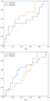 |
Fig. A.1. Cumulative distributions of fperi, the fractional distance in time between the pericentre (fperi = 0) and the apocentre (fperi = 1), for the on-plane (orange solid lines) and off-plane (blue solid lines) samples, considering values obtained with the low-mass (top panel) and high-mass (bottom panel) MW potentials. Dashed lines represent the expectation of a uniform distribution for each sub-sample. |
In Figs. A.2 and A.3, we show instead the comparison between orbital parameters (i.e. pericentre, apocentre, eccentricity, time since the last pericentre) calculated using a low-mass and high-mass MW potential, respectively. We remind to Sect. 4 for more details and Table 3 for the results of the statistical tests performed on the considered parameter distributions.
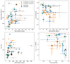 |
Fig. A.2. Comparison of the orbital properties for our sample of dwarf galaxies, assuming a low-mass potential for the MW. Top left: pericentre versus apocentre (in kpc). Top right: pericentre (in kpc) versus eccentricity. Bottom left: pericentre (in kpc) versus the half-light radius Re (in pc). Bottom right: eccentricity versus the orbital phase (i.e. the time since the last pericentric passage normalised by the orbital period). In all panels, symbols and colours are as described in Fig. 3. An arrow in the error bars indicates that a target lack a complete orbital solution and therefore the reported value is the calculated 16th quantile. |
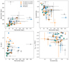 |
Fig. A.3. As in Fig. A.2, but with the orbital parameters derived assuming a high-mass potential for the MW. |
In Sect. 5.3, we discussed the effect of dynamical friction on the orbital properties of the brightest satellites of the MW on the VPOS. In Fig. A.4, we show their orbital evolution integrating backwards in time for 10 Gyr assuming the MWPotential2014 (Bovy 2015) and taking into account the effects of dynamical friction (assuming a varying ln(Λ(r)) and a scale radius for the dwarfs of 5 kpc, see e.g. Iorio et al. 2019). For the satellites total mass we assumed four values of MS = (5 × 10⁹; 1010; 5 × 10¹⁰; 1011) M⊙, compatible with abundance matching expectations for such luminous systems (e.g. Bullock & Boylan-Kolchin 2017). We see that the effects of dynamical friction start to be significant at MS ≥ 5 × 10¹⁰ M⊙.
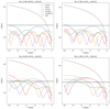 |
Fig. A.4. Orbital evolution of the bright dwarfs of the VPOS integrating backwards in time for 10 Gyr assuming the MWPotential2014 (Bovy 2015) and taking into account the effects of dynamical friction, assuming that the satellites have all a total mass of MS = 5 × 10⁹ M⊙ (top left), MS = 1010 M⊙ (top right), MS = 5 × 10¹⁰ M⊙ (bottom left), and MS = 1011 M⊙ (bottom right); the black solid line in all panels represents the MW virial radius rvir = 245 kpc. |
In Figs. A.5 and A.6, we also show the impact of uncertainties on the orbit recovery of each considered galaxy by performing 100 random realisations sampling from their position-velocity vector. We show in figures the results for two mass limits indicating on one side a typical value for these dwarf galaxies and on the other the minimum mass at which the effect of dynamic friction starts to be significant. We see that in most cases the errors mainly affect the orbital period rather than the amplitude, although for Carina and Fornax a fraction of the recovered orbits are unbound. This means that, in general, the number of pericentric passages tends to be conserved, even if the time at which they occur is the more uncertain the further back in time one integrates (particularly for times prior to 6 Gyr ago).
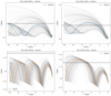 |
Fig. A.5. As in Fig. A.4, but here showing the impact of uncertainties on the orbital evolution of the individual systems. For each galaxy, we show as grey lines 100 realisations made by a Monte-Carlo sampling of the position and velocity vector, taking into account errors on distance, proper motion and radial velocity. We show results assuming that the satellites have a total mass of MS = 5 × 10⁹ M⊙ (left panels) and MS = 5 × 10¹⁰ M⊙ (right panels); the black solid line in all panels represents the MW virial radius rvir = 245 kpc. |
Finally, in Figs. A.7 we show the orbital evolution of the selected satellites in the Galactocentric Cartesian Y − Z, approximately coinciding with the one defined by the VPOS. We show orbits up to 4 Gyr ago for MS ≤ 1 × 10¹⁰ M⊙ (roughly the time to complete an orbital period) and up to 6 Gyr ago for MS ≥ 5 × 10¹⁰ M⊙ (roughly the time of entry into the MW potential). We see that within the errors, and especially at high masses (MS ≥ 5 × 10¹⁰), it is possible for the co-orbiting systems to share a common location in the past, however, the errors are too large to reach any significant conclusion. As wrote in the main text, a dedicated a dedicated study involving cosmological simulations is necessary to prove the hypothesis of a group infall origin for the VPOS.
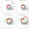 |
Fig. A.7. Panels as in Fig. A.4, but here showing the orbital evolution of the selected satellites up to 4 Gyr ago in the Galactocentric Cartesian Y − Z plane, which roughly coincides with the one defined by the VPOS. For each galaxy, we also show the orbits obtained from the 100 realisations made by Monte-Carlo sampling of the position and velocity vector, as in Fig. A.5. The circle in each panel has the same radius as the virial radius of the MW, rvir = 245 kpc. |
All Tables
Positions, velocities, and orbital poles of the MW satellites considered in this work.
All Figures
|
Fig. 1. Distribution of orbital poles in Galactic coordinates for the analysed sample of MW satellites. The median orbital poles are shown as open black circles, while the values of 5000 Monte Carlo realisations drawing on measurement uncertainties are shown as coloured dots. The colour scheme follows the division of our sample into on-plane (orange dots), off-plane (blue dots) and uncertain systems (grey dots) detailed in Sect. 2. |
| In the text | |
|
Fig. 2. Sub-sample selection. Left: distribution of the fraction fVPOS of Monte Carlo realisation for the orbital poles of our systems that are found within the VPOS area (i.e. within θVPOS = 36.87° from the orbital pole of the VPOS normal). Right: distribution of the V-band luminosity values for our systems as a function of their Galactocentric distance. In both panels, the on-plane systems are plotted in orange, the off-plane ones in blue, while systems with intermediate fVPOS are marked in grey. In the right panel, they are plotted using filled triangles (pointing up or down depending on whether a system is co- or counter-orbiting within the VPOS), circles and squares, respectively. In addition, black circles indicate the MCs and likely associated satellites, while green circles mark those systems that are in the off-plane sample independently of their proper motions. |
| In the text | |
|
Fig. 3. Comparison of the physical properties for our sample of dwarf galaxies. Top left: V-band luminosity LV versus the half-light radius Re. Top right: LV versus the global average metallicity [Fe/H]; the green band is the LV-[Fe/H] relation from Kirby et al. (2013). Bottom left: Re versus the velocity dispersion σv. Bottom right: luminosity Lhalf at the half-light radius versus the calculated dynamical mass Mhalf at the same radius; dashed black lines indicate constant M/L ratios of 1000, 100, 10 and 1, from left to right. In all panels, on- and off-plane systems are represented by orange triangles and blue circles, respectively, while uncertain systems are represented by grey squares. The LMC and its probable satellites are marked with black circles, while green circles mark systems being in the off-plane sample independently of their proper motions. |
| In the text | |
|
Fig. 4. Correlation matrixes showing Spearman’s rank coefficients between the inspected physical (luminosity, half-light radius, global average metallicity, velocity dispersion) and orbital parameters (pericentre, apocentre, eccentricity, time since the last pericentric passage) in the case of a low (left panel) and high (right panel) mass MW potential. In both cases, the upper right part corresponds to values for the on-plane sample, while the lower left part is for the off-plane sample; orange and blue shades correspond to the numerical values shown, with darker shades corresponding to a stronger correlation. |
| In the text | |
|
Fig. 5. Cumulative luminosity distribution of the satellites on-plane (orange solid line) compared to those off-plane (blue solid line); the distribution of the uncertain systems is reported too for comparison (grey solid line); dashed lines show the same comparison but removing the MC system. The grey band indicates the search completeness on the SDSS footprint (Koposov et al. 2008; Walsh et al. 2009; Simon 2018). |
| In the text | |
|
Fig. 6. Inspection of the velocity vector components. Left: median angular difference θVPOS between the orbital poles and the VPOS normal for our sample of MW satellites, as a function of their Galactocentric radial velocity Vrad; the red solid line is for reference only, since it helps to identify satellites that are approaching the MW (Vrad[km s−1] < 0) or receding from it (Vrad[km s−1] > 0); the red dashed lines represent the aperture angles around the two opposite poles of the VPOS. Right: θVPOS as a function of the |
| In the text | |
|
Fig. 7. Inspection of the orbital parameters. Top: time to the next or since the last pericentric passage, tperi, as a function of the satellites’ orbital period, P, both in units of Gyr; the red solid line at tperi = 0 indicate when satellites are at pericentre, the thin dashed lines indicate the apocentre limits, while the dotted lines mark the half-orbit; the thick dashed line, shown for illustrative purposes, is parallel to the upper apocentre line, shifted by ∼1 Gyr. Bottom: satellite orbital phases, ϕ, as a function of the orbital eccentricity; thin dotted lines represent the limits when a satellite has just left its pericentre (ϕ close to 0), or is approaching it (ϕ close to −1). Panels on the left show values obtained with the low-mass MW potential, while those on the right with the high-mass MW potential. In all panels, symbols and colours are as described in Fig. 3. |
| In the text | |
|
Fig. 8. As in Fig. 7, but considering results obtained with a MW potential perturbed by a massive LMC (see details in Sect. 4.3), in the top panel is shown the time to the next or since the last pericentric passage, tperi, versus the satellites’ orbital period, P, while in the bottom panel the satellites’ orbital phases, ϕ, versus the orbital eccentricity. We note that while some systems have a measured tperi, they may not have a closed orbit and therefore have P = 0 (such as the LMC and its satellites). |
| In the text | |
|
Fig. 9. Inspection of the energy and angular momentum values. Left: total specific energy E (in units of 104 km s−1) versus the square of the specific angular momentum L (in units of 109 kpc2 km2 s−2) at the present time; dotted line represents the relation for a particle of negligible mass on a circular orbit. Right: E against the specific angular momentum in the Cartesian x-direction of a Galactocentric reference frame, Lx (in units of 103 kpc km s−1); the red solid line at Lx = 0 is for reference only. In both panels, symbols and colours as in Fig. 3; error bars for the uncertain systems, which are large, are not shown for clarity. |
| In the text | |
|
Fig. 10. Difference between the observed weighted-average ⟨[Fe/H]⟩ of our galaxies and the expected values at their luminosity obtained from the Kirby et al. (2013) relation; symbols and colours as in Fig. 3. Error bars obtained adding in quadrature the errors on ⟨[Fe/H]⟩ and the rms = 0.17 dex of the Kirby et al. relation for the MW satellites. Dashed lines are the median offsets of each sub-sample. |
| In the text | |
|
Fig. 11. As in Fig. 9, but here including MW globular clusters (GCs) that probably formed in situ (brown hexagons) or were accreted, that is, associated with GSE/Sequoia (green diamonds), Sagittarius (red stars), or Helmi (purple pentagons) streams, according to the compilation of Massari et al. (2019). |
| In the text | |
|
Fig. 12. Orbital evolution of the bright dwarfs of the VPOS integrated backwards in time for 10 Gyr, assuming an evolving MW potential and taking into account the effects of dynamical friction, with the satellites assumed to have an individual total mass of MS = 5 × 10⁹ M⊙ (top panel) or MS = 5 × 10¹⁰ M⊙ (bottom panel). The black solid line represents the evolution of the virial radius of the MW. |
| In the text | |
|
Fig. A.1. Cumulative distributions of fperi, the fractional distance in time between the pericentre (fperi = 0) and the apocentre (fperi = 1), for the on-plane (orange solid lines) and off-plane (blue solid lines) samples, considering values obtained with the low-mass (top panel) and high-mass (bottom panel) MW potentials. Dashed lines represent the expectation of a uniform distribution for each sub-sample. |
| In the text | |
|
Fig. A.2. Comparison of the orbital properties for our sample of dwarf galaxies, assuming a low-mass potential for the MW. Top left: pericentre versus apocentre (in kpc). Top right: pericentre (in kpc) versus eccentricity. Bottom left: pericentre (in kpc) versus the half-light radius Re (in pc). Bottom right: eccentricity versus the orbital phase (i.e. the time since the last pericentric passage normalised by the orbital period). In all panels, symbols and colours are as described in Fig. 3. An arrow in the error bars indicates that a target lack a complete orbital solution and therefore the reported value is the calculated 16th quantile. |
| In the text | |
|
Fig. A.3. As in Fig. A.2, but with the orbital parameters derived assuming a high-mass potential for the MW. |
| In the text | |
|
Fig. A.4. Orbital evolution of the bright dwarfs of the VPOS integrating backwards in time for 10 Gyr assuming the MWPotential2014 (Bovy 2015) and taking into account the effects of dynamical friction, assuming that the satellites have all a total mass of MS = 5 × 10⁹ M⊙ (top left), MS = 1010 M⊙ (top right), MS = 5 × 10¹⁰ M⊙ (bottom left), and MS = 1011 M⊙ (bottom right); the black solid line in all panels represents the MW virial radius rvir = 245 kpc. |
| In the text | |
|
Fig. A.5. As in Fig. A.4, but here showing the impact of uncertainties on the orbital evolution of the individual systems. For each galaxy, we show as grey lines 100 realisations made by a Monte-Carlo sampling of the position and velocity vector, taking into account errors on distance, proper motion and radial velocity. We show results assuming that the satellites have a total mass of MS = 5 × 10⁹ M⊙ (left panels) and MS = 5 × 10¹⁰ M⊙ (right panels); the black solid line in all panels represents the MW virial radius rvir = 245 kpc. |
| In the text | |
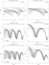 |
Fig. A.6. Figure A.5. Continued. |
| In the text | |
|
Fig. A.7. Panels as in Fig. A.4, but here showing the orbital evolution of the selected satellites up to 4 Gyr ago in the Galactocentric Cartesian Y − Z plane, which roughly coincides with the one defined by the VPOS. For each galaxy, we also show the orbits obtained from the 100 realisations made by Monte-Carlo sampling of the position and velocity vector, as in Fig. A.5. The circle in each panel has the same radius as the virial radius of the MW, rvir = 245 kpc. |
| In the text | |
Current usage metrics show cumulative count of Article Views (full-text article views including HTML views, PDF and ePub downloads, according to the available data) and Abstracts Views on Vision4Press platform.
Data correspond to usage on the plateform after 2015. The current usage metrics is available 48-96 hours after online publication and is updated daily on week days.
Initial download of the metrics may take a while.