| Issue |
A&A
Volume 684, April 2024
|
|
|---|---|---|
| Article Number | A147 | |
| Number of page(s) | 15 | |
| Section | Extragalactic astronomy | |
| DOI | https://doi.org/10.1051/0004-6361/202347423 | |
| Published online | 16 April 2024 | |
Polarimetry of the Lyα envelope of the radio-quiet quasar SDSS J124020.91+145535.6⋆
1
Institut de Physique, Laboratoire d’astrophysique, Ecole Polytechnique Fédérale de Lausanne (EPFL), Observatoire de Sauverny, 1290 Versoix, Switzerland
e-mail: pierre.north@epfl.ch
2
Stockholm University, Albanova University Center, Department of Astronomy, 106 91 Stockholm, Sweden
3
Kavli Institute for Particle Astrophysics and Cosmology and Department of Physics, Stanford University, Stanford, CA 94305, USA
4
Observatoire de Sauverny, Université de Genève, Chemin Pegasi 51, 1290 Sauverny, Switzerland
5
Kapteyn Astronomical Institute, University of Groningen, PO Box 800, 9700AV Groningen, The Netherlands
6
Univ. Lyon, Univ. Lyon 1, ENS de Lyon, CNRS, Centre de Recherche Astrophysique de Lyon UMR5574, 69230 Saint-Genis-Laval, France
7
Department of Physics, Faculty of Natural Sciences, University of Haifa, Haifa 31905, Israel
Received:
11
July
2023
Accepted:
5
January
2024
The radio quiet quasar SDSS J1240+1455 lies at a redshift of z = 3.11, is surrounded by a Lyα blob (LAB), and is absorbed by a proximate damped Lyα system. In order to better define the morphology of the blob and determine its emission mechanism, we gathered deep narrow-band images isolating the Lyα line of this object in linearly polarized light. We provide a deep intensity image of the blob, showing a filamentary structure extending up to 16″ (or 122 physical kpc) in diameter. No significant polarization signal could be extracted from the data, but 95% probability upper limits were defined through simulations. They vary between ∼3% in the central 0.75″ disk (after subtraction of the unpolarized quasar continuum) and ∼10% in the 3.8 − 5.5″ annulus. The low polarization suggests that the Lyα photons are emitted mostly in situ, by recombination and de-excitation in a gas largely ionized by the quasar ultraviolet light, rather than by a central source and scattered subsequently by neutral hydrogen gas. This blob shows no detectable polarization signal, contrary to LAB1, a brighter and more extended blob that is not related to the nearby active galactic nucleus (AGN) in any obvious way, and where a significant polarization signal of about 18% was detected.
Key words: quasars: emission lines / quasars: general / quasars: individual: SDSS J124020.91 + 145535.6
© The Authors 2024
 Open Access article, published by EDP Sciences, under the terms of the Creative Commons Attribution License (https://creativecommons.org/licenses/by/4.0), which permits unrestricted use, distribution, and reproduction in any medium, provided the original work is properly cited.
This article is published in open access under the Subscribe to Open model. Subscribe to A&A to support open access publication.
1. Introduction
Diffuse gas around quasars and galaxies bears the testimony of several processes related to galaxy formation and evolution: outflows, due to, for instance, quasar feedback (Cicone et al. 2015), accretion of intergalactic gas (Luo et al. 2021), or tidal debris resulting from collisions (Xu et al. 2022). Giant Lyman-α nebulae or Lyman-α blobs (hereafter LABs) have been discovered at high redshift over the last three decades, either in isolation or around radio-loud and radio-quiet quasars (Heckman et al. 1991; Bremer et al. 1992; Hu et al. 1996; Lehnert & Becker 1998; Møller et al. 1998; Fynbo et al. 1999; Bunker et al. 2003; Villar-Martín et al. 2003; Matsuda et al. 2004, 2009, 2011; Weidinger et al. 2005; Christensen et al. 2006; Francis & McDonnell 2006; Cantalupo et al. 2007, 2014; Smith & Jarvis 2007; Smith et al. 2009; Hennawi et al. 2009; Zirm et al. 2009; Scarlata et al. 2009; Yang et al. 2009; Rauch et al. 2011, 2013; Willott et al. 2011; Zafar et al. 2011; North et al. 2012; Goto et al. 2012; Francis et al. 2013; Kashikawa et al. 2014; Martin et al. 2014a,b, 2015; Jiang et al. 2016; Fathivavsari et al. 2016; Borisova et al. 2016). They typically extend over tens of kiloparsecs, sometimes over more than 100 kpc.
The origin of the emission of these objects has been much debated. Some authors (e.g., Caminha et al. 2016; Geach et al. 2016) attribute it to star formation and resonant scattering of Lyα photons. Others propose that photoionization by a central AGN is the main cause (Haiman & Rees 2001), even though an AGN is not detected at first sight in many LABs (Geach et al. 2009; Overzier et al. 2013; Schirmer et al. 2016; Kawamuro et al. 2017). Cabot et al. (2016) argued that the emission is due to collisional excitation of gas that is shock-heated by supernovae and gravitational accretion. Cooling radiation is also invoked, where cool streams of gas falling into the potential well of the forming galaxy release gravitational binding energy, which finally excites the hydrogen atoms (Haiman et al. 2000; Fardal et al. 2001; Nilsson et al. 2006; Dijkstra & Loeb 2009; Rosdahl & Blaizot 2012; Smailagic et al. 2017). Daddi et al. (2022) found some evidence for that. On the other hand, a Lyα nebula that was long considered as the most convincing example of gravitational cooling (Nilsson et al. 2006) is probably illuminated by a nearby buried AGN (Prescott et al. 2015; Sanderson et al. 2021).
Linear Lyα polarization was predicted as a diagnostic to infer the nature of the Lyα emission in LABs; scattered emission may be polarized (depending on the H I column density and number of scattering events), while in situ emission is not (Dijkstra & Loeb 2008). These theoretical predictions were refined in the context of gravitational cooling Lyα production, where simulations by Trebitsch et al. (2016) showed that gravitational cooling conserves some polarization in the Lyα nebulae. This is because, even though most Lyα photons are produced in situ, they are emitted mostly in the central, densest region of the nebula, so that a non-negligible part of them reach the outskirts of the nebula where they are scattered onto the observer.
The first attempt at detecting the polarization in a LAB (object LABd05 discovered by Dey et al. (2005), which contains an obscured AGN) could only put an upper limit of a few percent on the polarization fraction (Prescott et al. 2011). Using a larger telescope (the MMT-6.5m instead of the Bok-2.3m) and a more sophisticated imaging technique, Kim et al. (2020) later found a clear polarization signal in the same object. Hayes et al. (2011) managed to detect significant polarization in the bright LAB1 blob in the SSA22 protocluster (Steidel et al. 2000) on the basis of imaging polarimetry. Using the same technique, You et al. (2017) also detected significant polarization along the radio lobes of a radio galaxy. These results suggest that Lyα photons are not produced in situ, but rather near the center of the nebula, and scattered by neutral hydrogen towards the observer. Interestingly, Geach et al. (2014) observed an Ultra Luminous InfraRed Galaxy (ULIRG) with the James Clerk Maxwell Telescope (JCMT) at the center of the polarized pattern and concluded that this galaxy may well be the source of the Lyα photons scattered by the nebula. It was subsequently resolved with the Atacama Large Millimeter/Submillimeter Array (ALMA) into three components (Geach et al. 2016), and the main conclusion remains, that active star formation in these galaxies provides the necessary amount of Lyα photons to explain the nebula emission. Chapman et al. (2005) also showed that SubMillimeter Galaxies (SMGs; which are dusty starbursts similar to ULIRGs) often display Lyα in emission. The polarization fraction P is maximum for a scattering angle of π/2, so the observed fraction is expected to increase with the projected distance from the LAB center, and this is indeed observed, with P reaching ∼20% at a radius of 6 − 7″. Furthermore, the polarization vector is expected to be oriented tangentially (i.e., in a direction perpendicular to that of the source of Lyα photons), which is also observed. Beck et al. (2016) confirmed these results using spectropolarimetry and found indication of outflow.
Significant polarization (P = 16.4 ± 4.6%) was found in part of an extended Lyα nebula surrounding a radio galaxy (Humphrey et al. 2013), showing yet another example where scattering of Lyα photons by neutral hydrogen is important. Similarly, You et al. (2017) find, in a blob surrounding a radio-loud AGN, P < 2% at ∼5 kpc from the AGN and P ≃ 17% 15 − 25 kpc from it; polarization is detected along the major axis of the blob. Most recently, Kim et al. (2023) reported the detection of significant polarization in three out of four LABs hosting an AGN.
In this work, we focused on the LAB surrounding the radio-quiet quasar (RQQ) SDSS J124020.91+145535.6. As shown by Hennawi et al. (2009), this object is associated with a proximate damped Lyα system (PDLA), which acts as a natural coronagraph suppressing the quasar light around the redshifted Lyα wavelength. Such a providential geometry eases the observation of the faint LAB. As the quasar provides an obvious source of Lyα photons that may be scattered by the hydrogen atoms of the LAB, SDSS J124020.91+145535.6 appeared as a natural target for imaging polarimetry through a narrow band (NB) filter centered on the Lyα line. This is the first attempt at observing the polarization of a LAB centered on a quasar that is not radio loud1.
The observations are described in Sect. 2.1 and the results are presented in Sects. 3 and 4. The results are discussed assuming a cosmology with H0 = 70 km s−1 Mpc−1, ΩM = 0.3, and ΩΛ = 0.7. The magnitudes are reported in the Vega photometric system.
2. Observations and their reduction
2.1. Observations
The observations were carried out on 1-7 March, 2014 with the FOcal Reducer and low dispersion Spectrograph (FORS2) instrument (Appenzeller et al. 1998) attached to VLT-UT1. The FORS2 instrument was used in the imaging polarimetric (IPOL) mode: after passing through the collimator, the light beam goes through a Wollaston prism where it is split into two beams (the ordinary and extraordinary ones) with orthogonal polarizations. For the two images to be visible without overlapping one another, a strip mask is placed before the Wollaston prism, removing half the field of view, the full extent of which is 6.8′×6.8′. The strips are 22″ wide, which is more than the expected size of our object. Then, the beam goes through a half wave plate (HWP) that rotates the plane of polarized light. This plate can be rotated around the optical axis, and the images corresponding to the two beams are registered for four angles: 0, 22.5, 45, and 67.5 degrees, allowing us to recover both the degree and direction of the linear polarization at each point of the observed object. The narrow band (NB) filter OIII+50 was introduced into the beam to select the Lyα emission, because its central wavelength is perfectly suited to the redshift of the target. The quasar has zqso = 3.1092 ± 0.0014, based on the Hβ and [O III] emission line regions, while the Lyα emission line is at zLyα = 3.113 ± 0.001 (Hennawi et al. 2009); this corresponds to a velocity difference of 277 km s−1. The redshifted nebular emission corresponds to a wavelength λ0 = 5000.05 Å, almost right on the mean wavelength (5001 Å) of the OIII+50 ESO filter. With FWHM = 57 Å, this filter is wider than the emission Lyα line (FWHM ∼ 8 Å, see Fig. 1 of Hennawi et al. 2009), so its blue and red wings clearly include part of the quasar flux, even though it is strongly attenuated by the saturated Lyα absorption of the PDLA. This raises the question of whether the quasar continuum may blur the polarization signal; we address this question in Sect. 4.
A dithering pattern was adopted in the east-west direction, which was parallel to the x-axis of the CCD detector and to the long axis of the mask strips. Dithering in the other direction would have led to a possible loss of information, since the width of the strips are not much larger than the possible size of the Lyα blob. We used the blue-sensitive EEV detector, because it is slightly more efficient at 5001 Å than the MIT detector; this is why we observed in visitor mode.
In total, 100 exposures (i.e., 25 per HWP angle) were secured in dark time (no Moon) and photometric conditions through the NB filter in the IPOL mode, each with an exposure time of 500 s. The 1-σ noise in the background of each exposure is about 6 ADU, clearly dominating the read-out noise (RON), which amounts to 2.2 ADU. The airmass varied between 1.30 and 1.50 for 83 of them, and between 1.50 and 1.85 for the 17 remaining ones. The seeing measured on the frames varied from 2.5 pixels or 0.63″ to 4.2 pixels or 1.05″. On the combined intensity image, we measure a seeing of 0.76″.
We also devoted about half an hour to secure eight exposures through the wide-band vHIGH filter, each with an exposure time of 200 s, totaling 26 m,40 s. The airmass varied between 1.34 and 1.39, and the seeing measured on the combined image is 0.7″. Dithering was made in both the x and y directions. The deep image resulting from the coaddition of all these frames is important for distinguishing sites with continuum emission from those with Lyα emission.
2.2. Reduction
The reduction was made first using the FORS2 ESO pipeline (version 4.12.8) in the +gasgano+ (version 2.4.5) environment to make the master bias and the master sky flat-field NB frames. The sky flat fields were obtained without the Wollaston prism, HWP, and strip mask, because including the polarization optics would be impractical, and is not required in view of the observation strategy, as explained by Hayes et al. (2011, in the Supplementary information section).
Only the data registered by the CHIP1 (Norma III) CCD was reduced, because the quasar image always lies on that chip. Regarding the broad-band vHIGH data, we also focused on the CHIP1 frames, because half the CHIP2 (Marlene) images were corrupted for some unknown reason. We used the +forsimgscience+ recipe of the ESO FORS2 pipeline to reduce the vHIGH CHIP1 images. For the polarized NB images, the pipeline does not apply, so we had to use the +iraf+ command +imarith+ to subtract the bias level and the master bias, and divide by the master sky flat field. For the NB images, we subtracted the sky in a preliminary way using the +sextractor+ code with a smoothing on 200 pixels. This subtraction was only approximate because slight but systematic and significant differences in the sky level (up to ∼1 ADU) occur between the ordinary and extraordinary beams. Then, we corrected the intensities to unity airmass, using the average Paranal extinction coefficients listed in Patat et al. (2011, Table 3); we further scaled all images to the same flux level using the bright star closest to the QSO (1′33″ from it) and close to the middle of CHIP1. To align the images, we applied the +alipy+ code written by Malte Tewes. The +alipy+ code applies an affine transform to the images. We note that scaling amounted to less than a pixel at most. We isolated the ten strips corresponding to the ordinary and extraordinary beams. For each observing sequence and each strip, we refined the sky subtraction for the eight subframes corresponding to the four angles and the two beams using +sextractor+ again.
Finally, the +iraf+ command +imcombine+ was applied to combine the aligned images, using the +comb=average+ and +reject=minmax+ options. The combination was made separately for each angle of the half-wave plate. The same procedure was applied to the intensity vHIGH images, resulting in a full image instead of five 22″ wide strip.2 The result is shown in Fig. 1, where the NB intensity images were obtained by further combining the eight subimages related to the four angles and two beams.
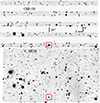 |
Fig. 1. Field covered by the CHIP1 detector, through the NB filter and through the wide-band filter. Upper panel: total intensity image in redshifted Lyα band, obtained by coadding all images corresponding to all four polariser angles and to both ordinary and extraordinary beams, as recorded on the CHIP1 detector. The total equivalent exposure time is 13 h, 53 min, and 20 s. The five bands correspond to the positions of the ordinary beam; the bands where the extraordinary beam falls appear blank here, because the corresponding images have been aligned and stacked with those of the ordinary beam. This shows that only half of the field is accessible in the polarization mode. The red square indicates and surrounds the LAB image, which includes the overexposed QSO near its center. The black circles designate objects detected at each angle and beam, and for which the polarization was measured. The red segments are the polarization vectors for objects with a polarization fraction of P > 5 σ. Lower panel: total vHIGH intensity image, corresponding to a total exposure time of 26 min, 40 s. The same red square as in the upper panel identifies the QSO. Both frames have the same scale. |
2.3. Flux calibration
2.3.1. Magnitude of the quasar through the vHIGH filter
We first verified that the quasar flux measured on our vHIGH images fits the magnitude V = 19.57 well (Véron-Cetty & Véron 2010). The magnitude obeys the relation
where N is the electron count, texp the exposure time, m0 the instrumental zero point, and K(vHIGH) the extinction coefficient. On the combined (averaged) vHIGH image, we measure N = 534681 e− for texp = 200 s, and the zero point is m0 = 28.19 in February-March, 2014 for zero airmass according to the ESO QC1 database.3 We adopted the average extinction coefficient K(vHIGH) = 0.128 (Patat et al. 2011) and obtain airmass = 1.37. With these numbers, we obtain vHIGH = 19.45, brighter than the catalog value. Actually, the zero point certainly refers to the standard MIT detector rather than the EEV one we used, but at the mean wavelength of the vHIGH filter (λ0 = 5550 Å), the quantum efficiency of the EEV detector is only about 5% higher than that of the standard MIT one (Boffin et al. 2013, Fig. 2.6). One would then expect the corresponding zero point to be about 0.05 magnitudes deeper for the EEV detector, changing our magnitude to 19.50. This is about 0.07 mag brighter than that listed in Véron’s catalogue.
2.3.2. Absolute flux through the NB filter
To calibrate our images in flux, we made use of the unpolarized spectrophotometric standard EG274≡WD 1620-391 (Hamuy et al. 1992) that was observed on March 4, 2014 at 05:46 UT through polarization optics under photometric conditions. It was observed four times by strongly variable seeing, each time through all four angles. Retaining the images with the best seeing4, we see that an 68 638 ADU s−1 count rate (obtained by integrating the signal in an aperture of 17 pixels radius5, i.e., 4.27″, and correcting for a k = 0.156 atmospheric extinction, with airmass = 1.56) corresponds to an average flux of
computed through the filter transmission curve T(λ) kindly provided by ESO. Multiplying this flux by the filter “equivalent width” defined as  Å, one obtains a total flux of 8.0 × 10⁻¹² erg s−1 cm−2. Here, the 68 638 ADU s−1 count rate is measured in one beam (ordinary or extraordinary) and corrected to zero airmass. When only one beam is considered (and assuming unpolarized light), the conversion factor is then

with an uncertainty that we estimate to roughly 10%.
2.4. Polarization calibration
We computed the polarization fraction and angle (according to the formulae (13), (14), and (16); see below) of the polarized star Vela1 95≡Ve6 − 23≡GSC08169 − 004127, observed on March 3, 2014 through the NB OIII filter. The star image fell on the same position on the CCD as that of the J1240 QSO target. We obtained

where the angle θ has been corrected for the instrumental effect6εF ≃ 3.5° according to the relation θ = θobs − εF, and where the errors are estimated through simplified formulae (Fossati et al. 2007, Eqs. (4) and (9)). This is consistent with measurements made with the FORS1 instrument in the IPOL mode through the broad-band V filter by Fossati et al. (2007, P = 8.26%±0.05%, θ = 171.61 ° ±0.21°). More importantly, this is also consistent with observations made with the FORS2 instrument in the PMOS mode, which allows one to determine P and θ as a function of wavelength (Cikota et al. 2017). Indeed, both P and θ depend on wavelength, and the mean wavelength of the V filter is ∼5500 Å, while that of the OIII+50 ESO filter is 5001 Å. At the latter wavelength, P = 8.0%±0.1% and θ = 172.8 ° ±0.3° (Cikota et al. 2017, Figs. 3 and 6). Thus, our measurements recover P to within the 1-σ error bars.
To assess the lack of substantial instrumental polarization, we also considered the non-polarized star WD1620-391, which has been measured through both the OIII+50 NB filter (on March 2, 2014) and the ESO bHIGH wide-band filter (on March 4, 2014). Through the OIII+50 filter, we obtained P = 0.11%±0.15% and 0.18%±0.15% for the two measurements with good seeing, while we obtained P = 0.07%±0.07% through the vHIGH filter. Likewise, the unpolarized star WD1615-154 observed through the OIII+50 filter on March 5, 2014 gives P = 0.45%±0.14% and 0.28%±0.14% for two measurements with excellent seeing. All this is compatible with zero polarization.
2.5. Polarized sources in the field
We applied the +Sextractor+ code to the average images corresponding to each of the two beams, four angles, and five 22″ bands registered on CHIP1. The polarization fraction and angle were computed (see formulae in Sect. 4) for each source detected in all average images, from the fluxes determined by +Sextractor+. The errors on the polarization fraction P were computed from the flux errors and corrected as explained in Sect. 4. The polarization angles were corrected for the instrumental effect mentioned in Sect. 2.4. The results are listed in Table A.1 for all objects, and shown only for objects with P > 5 σ(P) as red segments in Fig. 1.
The polarization of some objects is very small and probably spurious, because the error estimate does not include systematic effects: such is the case of the very bright star to the west of the QSO, close to the right edge of the frame. On the other hand, several sources have large P values. Their spatial distribution in the field does not suggest any connection with the QSO, and the orientations of their polarization vectors seem random. The most polarized object in the field, however, is close to the QSO in the field, and its polarization vector is tangential relative to the direction of the QSO. Thus, one might speculate that, if this object was at the same distance as the QSO from us, its polarization could be due to scattering of the QSO Lyα radiation by its hydrogen halo. Measuring the redshift of this object would help settle the question.
3. Morphology, luminosity, and surface brightness
3.1. Subtraction of the quasar signal in the NB images
Part of the signal in the NB image is due to the quasar itself, because the filter is not narrow enough to exclude the wings of the saturated Lyα absorption of the PDLA. Therefore, we had to subtract this contribution before analyzing the properties of the LAB. Since there are four polarization angles, there are four combined NB images, each containing two subimages corresponding to the ordinary and extraordinary beams; this makes a total of eight subimages per polarization measurement sequence. In total, we obtained 25 exposures for each polarization measurement sequence. Co-adding those 25 exposures, the deepest possible intensity image reaches a 1-σ noise of ∼0.53 × 10⁻¹⁸ erg s−1 cm−2 arcsec−2 in the sky. The mean seeing of our data is 0.76 ″ FWHM.
The quasar/LAB light decomposition is performed as follows. First, the PSF is reconstructed using the STARRED PSF reconstruction and deconvolution Python package (Michalewicz et al. 2023). A subsampled (by a factor of 2) model of the PSF is generated for each exposure, and for each of the two beams and four position angles of the Wollaston plate by fitting the light profile of two bright stars in the field of view. STARRED obtains the best-fit model of the PSF by first adjusting a Moffat profile to those stars and then applying a pixelated correction, regularized with a wavelet. Second, we use STARRED to perform a two-channel deconvolution of the data in order to separate the quasar light from the extended emission. For each of the two beams and four position angles, we perform a joint deconvolution of all the 25 exposures using individually reconstructed PSFs in each image. STARRED models the quasar as a point source and the LAB extended emission as a wavelet-regularized pixel grid. These two channels are jointly fit to the data. The amplitude of the point source and a spatially constant sky correction is free to vary between individual exposures, whereas the extended emission channel is kept constant across all exposures. The reconstruction is performed at twice the resolution of the original data, and we also fit a small sub-pixel shift to all exposure to align the images. Finally, we subtract our best-fit point-source model to each of the images and stack the 25 exposures before performing our polarization measurement. STARRED also provides the photometry of the quasar for each beam and position angle. We measure a polarization for the quasar of P = 0.0052 ± 0.0053, which is consistent with previous measurements of radio quiet quasars. Indeed, while radio galaxies do show important polarization fractions of up to 0.15 − 0.20 (Cimatti et al. 1998; Vernet et al. 1999), most radio quiet quasars (like ours) have P < 0.01; according to Hutsemékers et al. (2014, Fig. 1), 86% of the RQQs have P < 0.01 and 97% have P < 0.02.
3.2. Morphology
The average intensity image is shown in Fig. 1 and reveals the shape of the blob. Interestingly, this deep exposure shows that, although the bright central part of the blob is no larger than ∼5″ as mentioned by Hennawi et al. (2009), fainter structures extend up to radii of ∼8″. Thus, the total extent of the blob reaches ∼16″, or 122 kpc (taking into account that 1″ corresponds to 7.615 kpc). With its complex and filamentary structure, this blob appears quite typical of those found around radio-quiet quasars using the MUSE integral field spectrograph (Borisova et al. 2016).
Several small and faint objects surrounding the blob are seen through both the OIII+50 and vHIGH filters and may be small galaxies. The faint patch at 8″ to the SW of the quasar has no counterpart on the vHIGH image. It may be a hydrogen cloud of the same kind as those detected by Cantalupo et al. (2012).
3.3. Luminosity of the blob
Within a radius of 30 pixels or 7.53″, the sum of the pixel values of the nebular emission amounts to 24.82 e− s−1 outside the atmosphere, and as a first approximation we consider it negligible beyond this radius. Applying the conversion factor fconv (Eq. (2)) and remembering that 1 ADU = 2.24 e−1, we obtain a total flux of

The uncertainty was set at ∼10%, essentially reflecting the uncertainty on the flux calibration. Interestingly, the intensity of the Lyα emission shows two maxima, one that occurs at the position of the quasar and another that is slightly offset by about 0.6″ to the east and 0.3″ to the south of the quasar. The positions of the quasar and of the secondary maximum are summarized in Table 1. Integrating the surface brightness profile fit to the data up to a 7.53″ radius (see below) resulted in the same value as that given above (Formula (4)), within 11%.
Characteristics of quasar SDSS J124020.91 + 145535.6 and position of the secondary maximum of the LAB intensity.
The luminosity distance is 26572 Mpc (Wright 2006).7 The luminosity of the blob is thus

a value close to the median one for the blobs in the sample of Borisova et al. (2016). Among the 17 blobs of this kind observed by these authors, seven are brighter than our object and ten are fainter.8 Besides, only one of the 14 LABs listed by Matsuda et al. (2011, Table 2), SSAA22-Sb3-LAB1, is brighter than that. We note that the two articles quoted here use the same cosmological parameters as we do.
3.4. Surface brightness
We obtain the surface brightness (SB) profile displayed in Fig. 2 by adding the pixel values in concentric annuli with increasing radii (the first “annulus” is a disk with radius r = 4 pixels, while the annuli proper are two pixels thick between r = 4 pixels and r = 6 pixels, one pixel thick between r = 6 pixels and r = 24 pixels, and two pixels thick between r = 24 pixels and r = 30 pixels). We adopted the quasar as the center of the photometric apertures.
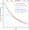 |
Fig. 2. Average surface brightness (SB) as function of radius. Each radius value is the arithmetic mean of the two bounding radii of the corresponding annulus (e.g., R = 2 pixels ≃ 0.5″ for the central R < 4 pixel disk and R = 5 pixels for the 4 ≤ R < 6 pixel annulus). The error bars represent the rms scatter of the pixel values in the corresponding annulus; it includes not only the shot noise, but also the cosmic SB variation within the annulus. The two red regression lines are those given by Eqs. (6) and (7). The black curve is the fit of a sum of two exponentials (Eq. (10)), while the green one is a Sérsic profile with index m = 6; the cyan curve is a stellar profile (see text). The solid blue line is the fit to the average SB profile of the 11 LABs considered by Steidel et al. (2011), while the broken blue line is the same for the 52 galaxies with Lyα in emission (Steidel et al. 2011). |
For comparison, in Fig. 2 we also show the SB profile of a star (equivalent to a PSF) in the same field of view and in the same strip as the QSO in the combined NB image. The star used lies at α(J2000) = 12 : 40 : 26.246 and δ(J2000) = + 14 : 55 : 27.7, and its SB within 2 pixels (r < 0.5″) was scaled to coincide with that of the LAB at same radius. The contrast between the two curves confirms the extended nature of the object.
The SB trend of the blob shows two linear parts in this logarithmic plot, the first within 3.4″ (26 kpc) with a steep slope and the second between 3.4 and 6″ (26 and 46 kpc) with a shallower slope.9 Assuming a halo mass between 1012 and 1013 M⊙ at z = 3.1, the virial radius would correspond to ∼80 − 170 kpc, so we are probing a region that is between 1/3 and 2/3 of the virial radius, for the most extended points. The error bars correspond to the rms dispersion of the pixel values within each annulus. Thus, they include not only the photon noise, but also the cosmic SB variation within the respective annuli, so they are larger than the error due to the shot noise alone. Although the annuli are disjointed, their SB and error bars are correlated because of the seeing.
The regression lines were fit using weighted least squares (the weights being the inverse of the variances, but neglecting the correlations) and obey the following laws:
![$$ \begin{aligned}&\log ({SB})=-15.997\pm 0.047-(0.348\pm 0.021)\cdot R\,[{\prime \prime }] ,\\&\qquad \qquad \quad \mathrm{for} ~~ R < 3.4^{\prime \prime } \nonumber \\&\log ({SB})=-16.596\pm 0.048-(0.167\pm 0.010)\cdot R\,[{\prime \prime }] ,\\&\qquad \qquad \quad \mathrm{for} ~~ 3.4^{\prime \prime } < R < 6^{\prime \prime }\nonumber \end{aligned} $$](/articles/aa/full_html/2024/04/aa47423-23/aa47423-23-eq8.gif)
with SB expressed in erg s−1 cm−2 arcsec−2. The rms scatter of the residuals is 0.049 and 0.020 dex for the inner and outer parts of the LAB, respectively. The SB beyond R = 6″ lies increasingly above the linear trend. Even though the last three points correspond to a very low SB, they probably represent a real flux, as suggested by the large, very faint structures still visible up to ∼8″ from the quasar in Fig. 1. Integrating Eqs. (6) and (7) up to R = 6″ results in a total flux of 1.06 × 10⁻¹⁵ erg s−1 cm−2, about 18% smaller than that obtained (Eq. (4)) from direct summation of the signal, as expected because some signal remains beyond R = 6″.
Taking into account that 1″ corresponds to 7.615 kpc, the SB can also be written as follows:
![$$ \begin{aligned}&{SB}=(10.08\pm 1-09)\cdot 10^{-17}\,\exp \left(-\frac{R\,\mathrm{[kpc]} }{9.51\pm 0.58}\right) ,\end{aligned} $$](/articles/aa/full_html/2024/04/aa47423-23/aa47423-23-eq9.gif)
![$$ \begin{aligned}&\mathrm{for} ~~ R < 26\,\mathrm{kpc} \nonumber \\&{SB}=(2.53\pm 0.28)\cdot 10^{-17}\,\exp \left(-\frac{R\,\mathrm{[kpc]} }{19.8\pm 1.2}\right) ,\end{aligned} $$](/articles/aa/full_html/2024/04/aa47423-23/aa47423-23-eq10.gif)

with R expressed in kpc and SB still expressed in erg s−1 cm−2 arcsec−2.
Although the double linear regression just described fits the data very well, it suffers from the drawback of an a priori definition of the regression limit in radius (3.4″) that is defined by eye in a rather subjective way. A more objective fit was performed to the sum of two exponential functions (actually to the decimal logarithm of it), giving:
![$$ \begin{aligned}&{SB}=(129.0\pm 8.0)\cdot 10^{-18}\cdot \exp \left(-\frac{R\,[{\prime \prime }]}{0.818\pm 0.051}\right) \nonumber \\&+(12.7\pm 2.9)\cdot 10^{-18}\cdot \exp \left(-\frac{R\,[{\prime \prime }]}{3.93\pm 0.61}\right) \,\mathrm {erg\,s}^{-1}\,cm^{-2}\,arcsec^{-2} , \end{aligned} $$](/articles/aa/full_html/2024/04/aa47423-23/aa47423-23-eq12.gif)
or, translating arcseconds into kiloparsecs,
![$$ \begin{aligned}&{SB} =(129.0\pm 8.0)\cdot 10^{-18}\cdot \exp \left(-\frac{R\,[\mathrm{kpc}]}{6.23\pm 0.39}\right)\nonumber \\&+(12.7\pm 2.9)\cdot 10^{-18}\cdot \exp \left(-\frac{R\,[\mathrm{kpc}]}{29.9\pm 4.7}\right) \,\mathrm {erg\,s}^{-1}\,cm^{-2}\,arcsec^{-2} , \end{aligned} $$](/articles/aa/full_html/2024/04/aa47423-23/aa47423-23-eq13.gif)
with an rms scatter of the logarithmic residuals of 0.031 dex. The relatively large errors on the fit parameters stem from the inclusion of the last three points, which have among the largest error bars, and from correlations between some parameters (in particular between the two amplitudes, and between the amplitude and scale of the second exponential term).
3.4.1. Comparison with other LABs and Lyα haloes of high-z galaxies
The SB profile of the inner part of our blob is thus much steeper than that of the 11 giant Lyα blobs considered by Steidel et al. (2011, Table 2, column 6), that have an e-folding radius10 of 27.6 kpc (i.e., more than three times larger). It is also steeper than the average diffuse Lyα− emitting halo of the 52 high-redshift star-forming galaxies (with net Lyα emission) studied by Steidel et al. (2011), which have a typical radius of 25.6 kpc, quite close to that of the giant blobs. On the other hand, the outer part of our blob has an SB profile closer to that reported by Steidel et al. (2011), though the uncertainty is large. Interestingly, the SB of the diffuse Lyα halos of the galaxies studied by Steidel et al. (2011, Figs. 5–8), also show a steep linear part (on a log scale) in the inner region and a less steep linear relation in the outer region, the break occurring between 25 and 30 kpc, which is only slightly more than in our object. This is intriguing, because Steidel’s galaxies generally do not currently host any active nucleus, in contrast to SDSS J124020.91+145535.6. On the other hand, the surface brightness of our object is typically an order of magnitude higher than that of Steidel’s objects. This can be interpreted in two ways. First, while Steidel’s objects are representative of L ≃ L⋆ Lyman break galaxies (LBG), our object is likely representative of more luminous galaxies, since it hosts a quasar (Hutchings et al. 1984; Smith et al. 1986; Percival et al. 2001; Hamilton et al. 2002; Hyvönen et al. 2007; Falomo et al. 2014). Second, the quasar that is present in our object but not in Steidel’s probably enhances the nebular Lyα emission by photoionizing hydrogen (Overzier et al. 2013; Chelouche et al. 2008).
The LAB1 object, which seems to be included in Steidel’s sample of 11 giant LABs, was studied in detail by Hayes et al. (2011). It has an e-folding radius of about 20 kpc beyond ∼2″, close to the average of the 11 LABs. As the latter, it does not show the double exponential behavior that is present in both our object and Steidel’s stacked galaxies.
Wisotzki et al. (2016) observed 26 Lyα-emitting galaxies at large redshift (3 < z < 6) with the MUSE spectrograph and detected a Lyα halo around most of them. The SBs of these haloes follow an exponential law, but with a typical characteristic length of only a few kiloparsecs. Leclercq et al. (2017) confirmed this result on a much larger sample of star-forming galaxies, finding an average scale length of 4.5 kpc. They are much less extended than our object.
These comparisons remain limited by the unknown contribution of a possible UV continuum, especially near the center of the object. Nevertheless, the SDSS spectrum displayed in Fig. 1 of Hennawi et al. (2009) corresponding to R < 1.5″ suggests that such a continuum is small, if any.
3.4.2. Comparison with other quasar Lyα haloes
Interestingly, discarding the central SB and plotting log(SB) against log R leads to an almost linear relation with a slope −1.68 ± 0.03 (Fig. 3), in fair agreement with the average slope of −1.8 found by Borisova et al. (2016) for 17 blobs surrounding bright radio quiet quasars. Borisova et al. (2016) consider only the range R > 10 kpc, just as in our Fig. 3, and find that a power law better fits their data than a single exponential.
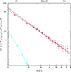 |
Fig. 3. Same as Fig. 2, but with a logarithmic scale on both axes, and starting only from R = 1″. The regression line shown in magenta is computed from the red dots displayed here, discarding the dot at R ≃ 4 kpc. The black line shows the power law with an index −1.8, corresponding to the average SB profiles of the blobs studied by Borisova et al. (2016). The stellar profile is shown in cyan. |
The reason why a power law appears more satisfactory to Borisova et al. (2016) may be due to their blobs obeying a double exponential law, as is the case of our object. It would be interesting to reanalyze their data and look how far a double exponential is able to fit them.
3.4.3. Other possible fits to the SB radial profile
We tried to adjust a Sérsic profile,
![$$ \begin{aligned} {SB}(R)=I_\mathrm{e} \,\exp \left(-b_\mathrm{m} \left[\left(\frac{R}{R_\mathrm{e} }\right)^\mathrm{1/m}-1\right]\right) ,\end{aligned} $$](/articles/aa/full_html/2024/04/aa47423-23/aa47423-23-eq14.gif)
where Re is the half-luminosity radius and Ie is the surface brightness at that radius. We used Eq. (10) to determine these two parameters: Re = 2.73″, Ie = 10.9 ⋅ 10−18erg s−1 cm−2 arcsec−2. We also used the relation bm = 2m − 0.324, which is a very good approximation to the real one (Binney & Tremaine 2008; Ciotti & Bertin 1999). For all Sersic indices m = 2 − 6, the fit is acceptable for R ≥ 1.7″, but the central intensity of the profile diverges to values far above the measured one. The profile for m = 6 is shown on Fig. 2. This type of profile clearly does not fulfill the observational constraints.
3.5. Central part: The PDLA against the diffuse Lyα background
The LAB structure is shown in more detail in Fig. 4. The left panel shows the faint extended features, while the central panel shows the inner part of the LAB. The red circle shows the position of the quasar that has been subtracted through the deconvolution process. The right panel shows the stacked residuals left by the deconvolution, after subtraction of both the extended and point-source components.
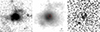 |
Fig. 4. Central structure of LAB, with north up and east left. On the left is the extended low-surface-brightness structures around the quasar. The middle panel shows a zoomed-in view of the central parts after subtraction of the point-source component of the image following the deconvolution of all frames with STARRED. The image is a stack of all quasar-subtracted images (see text) and the position of the point-source component is shown as a red circle. This image is at the spatial resolution of the original data. We note the double structure of the flux distribution. The north-west maximum corresponds to the position of the quasar that has been subtracted, while the SE maximum has no direct connection with the quasar. The right panel shows the stacked residuals with cut levels spanning −3σ to +3σ. We note that while a structure is seen in the center, it is quantitatively negligible. |
The middle panel of Fig. 4 reveals that the central part of the LAB does not present a single maximum, but rather a bimodal structure with one maximum coinciding with the quasar position and another maximum to the south-east of it. These two positions are summarized in Table 1. The reason for this asymmetry is unclear. Hennawi et al. (2009) suggested that we might be seeing the PDLA silhouetting against the bright background. These authors argued that star formation in the PDLA cannot account for the extended Lyα emission in H II regions, unless it is unrealistically large. They also argue that fluorescent recombination radiation taking place in the PDLA ISM and powered by the quasar cannot be invoked either, because the optically thick gas giving rise to the Lyα emission shields the same radiation from the observer’s view. Thus, one may wonder whether the asymmetry of the flux distribution is related with the PDLA, that would block not only the Lyα flux of the quasar but also part of that of the LAB. Our data has not enough spatial resolution to clarify this point; it is compatible as well with a mere asymmetry of matter distribution within the LAB. The adaptive optics and narrow-field mode of the MUSE instrument is perfectly suited to explore the central region of this LAB, and it might be able to shed light on this issue.
4. Polarization
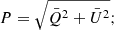
On the eight average images (corresponding to the four position angles and the two beams, each image reaching a depth corresponding to an rms dispersion of ∼1.5 × 10⁻¹⁸ erg s−1 cm−2 arcsec−2), we defined a circular region of 5.5″ radius centered on the quasar and divided it into five annuli and eight sectors (see Fig. 5, left panel). We summed the LAB intensity in each of the 40 resulting areas for each of the eight images. The average polarization fraction P was computed for each of the 40 sectors; the result is shown in Fig. 5. We used the following formulae:
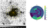 |
Fig. 5. Polarization signal in sectors of successive annuli of increasing radius around the quasar. Left: definition of the sectors on the average LAB image. The first “annulus” is actually a disk with a three-pixel (0.75″) radius, while the other annuli have an outer radius of 1.5, 2.5, 3.75, and 5.5″, respectively. The red segments indicate the polarization fraction through their length and the polarization angle through their orientation. The background image is a median stack of the 200 individual images corresponding to the two beams, four angles, and 25 exposures. The corresponding intensity bar is in electron units, representing the average flux received during 500 s and corrected for atmospheric extinction. Right: map of polarization fraction. The latter was corrected statistically using Eq. (A3) of Wardle & Kronberg (1974), but spurious polarization still appears in some sectors with low signal (e.g., the outermost one between 270 and 315°). |
 and
and  are the normalized Q and U Stokes parameters. They are related to the normalized flux differences Fθ defined as
through the relations
where the subscripts refer to the HWP angles expressed in degrees. The error on the polarization fraction obtained through propagation, under the assumption of Gaussian shot noise, negligible readout noise, and the same background level in the ordinary and extraordinary beams, reads
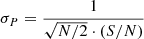
(Patat & Romaniello 2006), where N is the number of HWP angles (4 in our case), and S/N is the signal-to-noise ratio of an intensity image ( ). The polarization angle χ is given by the formula
and its error is given by
Because of the noise and of the intrinsically positive nature of the P quantity, the values taken by the latter are strongly biased when computed in the way described above. Wardle & Kronberg (1974) proposed a first-order statistical correction (their formula A3), which in our case takes the form
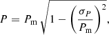
where P is the corrected polarization fraction, Pm is the “measured” polarization fraction computed through Eq. (13) and σP is the rms standard deviation of Pm due to background and photon noise, computed by the standard propagation formulae. This correction is included in the results shown in Fig. 5; it is clearly not sufficient, in view of the high P value in regions with very low or negligible flux.
Averaging the polarization fraction on azimut in each annulus, we obtain the trend shown in the left panel of Fig. 8. The error bars are simply the rms standard deviations of the eight P values available in each annulus divided by  ; they represent the error on the average polarization at given radius, under the assumption of a normal distribution of P values. Because the latter assumption is not valid, the apparent slightly positive trend only betrays the effect of noise, even though the latter has been partly cancelled by the correction mentioned above. The polarization fraction being defined by construction as a positive quantity, its frequency distribution is highly asymmetric even though the pixel intensities follow a Gaussian distribution around the mean value on the frames.
In order to quantify the uncertainties on P, we produced 10 000 artificial images of the LAB for each polarization angle and beam. Starting from a smoothed image of the blob in unpolarized light (smoothed by a Gaussian PSF with FWHM = 0.75″, similar to the seeing of the data), we added Poisson noise corresponding to the scatter measured on the background of the true image, and scaled it according to the signal intensity. Zero polarization was assumed, so that the artificial images corresponding to ordinary and extraordinary beams, and to the various angles, differ only by the added noise (i.e., by the different statistical realizations of the noise patterns, all realizations being drawn from the same parent noise distribution); we also assume here that the noise depends neither on the HWP angle nor on the beam (ordinary or extraordinary), and indeed the measured noise is the same to an accuracy level better than 10%. We then computed P in the same way as for the true images, including the Wardle & Kronberg correction. For each of the 5 × 8 = 40 sectors, we have determined the polarization fraction above which only 5% of the random draws occur. The resulting map of this limiting value is shown in Fig. 6; it may be considered as a map of the upper limits to P that we would obtain from ideal (i.e., free from any systematics) but noisy data such as ours, the limit corresponding to a 95% probability. We note that this map essentially reflects the surface brightness distribution of the LAB because of the anticorrelation between the spurious signal and the signal-to-noise ratio.
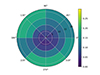 |
Fig. 6. Simulated map of limiting polarization fraction, which can be exceeded with only 5% probability. The statistical correction for the effect of noise was applied (see text). |
For each randomized set of images, the simulated polarization fraction was averaged in azimut in exactly the same way as for the observed data. This yields the set of five cumulative distributions shown on Fig. 7, each distribution corresponding to a different annulus. For example, the cumulative distribution for the outermost annulus (red curve) shows that half of the simulated data yield a “measured” polarization fraction P < 0.06 in this annulus, while the other half yield 0.06 < P < 0.15, so the median P value is 0.06. We see that both the mode and the width of the distributions increase with radius because of increasing noise linked with decreasing intensity. Even though the Wardle & Kronberg correction was applied, there is still an ∼5% probability of a polarization fraction P > 0.10 in the outer annulus. This is of course a spurious, apparent polarization due to noise alone, since zero polarization was assumed in the simulation.
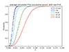 |
Fig. 7. Spurious “observed” polarization P due to noise in successive annuli of increasing radius around the quasar, according to simulations assuming zero real polarization. The limiting radii (inner and outer radius) of each annulus are given in the upper right box in pixel units; there are four pixels per arcsec, so the outermost radius (22 pixels) corresponds to 5.5″. The corresponding cumulative probability distributions are given. |
The “observed” polarization map shown in Fig. 5 appears more contrasted than the simulated one (Fig. 6) for the 95% limit, which is not unexpected, but it also displays some sectors exceeding that limit, most notably one in the outer annulus, and a few at smaller radii. One has to keep in mind that the simulation does not include any systematic error, while actually there is also some uncertainty on, for instance, the sky subtraction. Nevertheless, the two maps are roughly and globally consistent.
In the simulation (Fig. 7), the upper limit to the azimutally averaged P (with 95% significance) increases from ∼2% for a projected radius R < 1.5″ to ∼10% at R ≃ 4.6″. Observations (Fig. 8) lie below or close to this limit, and noise prevents us from determining meaningful P values beyond a radius R ∼ 5″ = 20 pixels. Therefore, we conclude that our data are compatible with no polarization up to about 5″ or 38 kpc from the quasar.
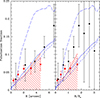 |
Fig. 8. Average polarization fraction in successive annuli as a function of radius. Left panel: radius expressed in arcseconds. Red dots: this work. The statistical correction for the effect of noise (see text) was applied. The error bars are the rms standard deviation of the P values in the eight sectors corresponding to each radius, divided by |

5. Discussion and comparison with theoretical simulations
Figure 8 also displays the polarization fraction found by Hayes et al. (2011) in LAB1 (black dots). At small radii, their results are not widely different from ours, but their object is brighter at large radii and their P values are significant there. They reach P ≃ 0.18 at about 6.7″ from the LAB center11. In our case, the flux beyond 5″ is too small to draw meaningful conclusions about larger radii.
The lack of significant polarization is surprising at first sight, in view of the simulations of synthetic blobs performed, for example, by Trebitsch et al. (2016). In their work, Trebitsch et al. (2016) considered two distinct sources of Lyα photons (see Fig. 8 and their Fig. 5): one related to the extragalactic component, made of gas with densities nH ≤ 0.76 cm−3, and one related to the galactic component, in the form of H II regions lying in the central galaxy. The former component includes the circumgalactic gas (CGM), cold streams and other diffuse gas, while the latter is made of galactic interstellar matter.
Based on the polarization measured by Hayes et al. (2011), we would expect a polarization level similar to that of the overall Lyα emission case (i.e., extragalactic and galactic components combined; solid blue line in Fig. 8). In such a situation, we expect P = 10.5% at R = 4.6″, while we find only 7%. At this radius, the prediction coincides with our 95% upper limit defined by the simulations described above; in the case of no true polarization, the measured polarization fraction has a 95% probability of falling below this limit (red line in Fig. 8). Trebitsch et al. (2016) predicted P ≃ 0.07 at the ∼3.1″ radius, above our 95% limit; their prediction also lies above the 95% limit at 2″ and 1.1″ radii. The only exception occurs for the innermost region, with an average radius of ∼0.4″, where we find P ∼ 0.028, slightly above the theoretical prediction but still below our 95% limit.
The short-dashed and long-dashed blue lines in Fig. 8 refer to the extragalactic and galactic components of the Lyα emission, respectively, that are envisaged by Trebitsch et al. (2016). Interestingly, the extragalactic emission is extended by definition; in other words, the Lyα photons are produced in situ, so no polarization is expected at first sight for this component. However, the CGM density decreases outwards, so most photons are produced near the LAB center and a significant fraction of them are scattered in the outer regions before reaching the observer, which explains the rather high predicted polarization fraction. Conversely, the photons corresponding to the galactic component are emitted exclusively near the LAB center12, where the galaxies lie, and many of them are subsequently scattered toward the observer, thereby acquiring their large polarization.
The fact that the P measurements fall in or near the 95% probability area makes any agreement with the theoretical prediction unlikely, especially as the orientation of the polarization vector is not systematically tangential. This remains true even if we consider only the extragalactic component (short-dashed curve in Fig. 8). This is even more striking if we consider the galactic component alone (long-dashed curve), that is, assuming no in situ extended emission. The observed extended emission can clearly not be due to the scattering of Lyα photons emitted by the quasar, since the polarization would then exceed 20% in the outer regions.
In this comparison with the simulated LAB, one has to keep in mind that the latter differs in some important respects from the real observed LAB, even though the redshifts are roughly the same. This holds not only for our object, but also for LAB1 observed by Hayes et al. (2011). The simulated LAB is much less luminous, with an SB about five times lower than our observed one out to radii of about 5 − 6″. Thus, if the polarization properties are tied to the gas distribution, comparing them at the same physical radius for widely different LABs may not be optimal. A rather natural way to compare different LABs is to plot P as a function of a radius normalized to the effective radii Re of the respective LABs (where Re is the radius encompassing half of the LAB total luminosity). We estimate Re = 2.79″ for SDSS J1240+1455, 3.71″ for LAB1, and 2.09″ for the simulated LAB; the polarization fraction is plotted as a function of the ratio R/Re in the right panel of Fig. 8. Because the effective radius of our LAB is not very far from that of the simulated one, little has changed compared to the left panel of Fig. 8; the simulated overall Lyα emission is now slightly below the observed P upper limit (red line). Conversely, all LAB1 data points (Hayes et al. 2011) now lie above the curve of the simulated LAB (continuous blue line), while they were fully compatible with it in the left panel of Fig. 8. They lie roughly halfway between the so-called galactic and overall emission curves, suggesting a larger contribution, in LAB1, of the galactic Lyα emission than of the extragalactic emission to the polarization.
One explanation for the difference between LAB1 and the simulation is the steeper SB profile (or smaller Re) of the latter. This steeper profile may be linked to the fact that the underlying cosmological simulation lacks feedback and metals, leading to a dearth of gas (including cold gas) in the CGM and eventually to an underestimated Re relative to a more realistic model. This would probably affect the polarization profile too.
Our object differs greatly from the simulation by the presence of a quasar; there is no AGN activity whatsoever in the simulation, and the ionizing radiation only comes from the UV background. This would also partly affect the radial H I profile, and consequently the Lyα and polarization profiles. Thus, we can interpret the observed polarization (or lack of it) in several ways. The gas may be largely photoionized by the quasar, so the Lyα emission may be essentially due to spontaneous emission following recombination, rather than to scattering of Lyα photons. Indeed, photoionization reduces the H I number density, hence the number of potential scatterers; thus, two mechanisms concur here to reduce polarization, compared to the simulated LAB that hosts no quasar. Another possibility is that, even if scattering does occur, the scattering angle never takes the π/2 value because the gas lies in front of, or behind the quasar instead of lying in the same plane perpendicular to the line of sight.
6. Conclusion
We present a detailed analysis of the LAB surrounding the radio-quiet quasar SDSS J1240+1455 using narrow-band imaging polarimetry. Taking advantage of the PDLA acting as a natural coronagraph, we were able to describe the morphology of the LAB and put an upper limit on its polarization fraction. This is the first polarization study of a LAB obviously hosting a radio-quiet quasar.
The main results can be summarized as follows.
-
The LAB shows a complex filamentary structure, which is typical of other LABs and that would be worth exploring further with an IFU instrument such as MUSE at VLT.
-
The LAB structure could be characterized down to its center, taking advantage of the coronagraphic effect provided by the PDLA. However, the filter was still too wide to completely exclude any light from the quasar, and subtracting this light was necessary, introducing some uncertainty. A bimodal structure was found in the LAB center that may be due either to a foreground absorption possibly linked to the PDLA or to some density fluctuation in the LAB itself. Here too, MUSE observations may shed light on the nature of this feature.
-
The azimuthally averaged surface brightness of the LAB decreases exponentially from its center, but with a steeper slope in the inner region than in the outer one.
-
No significant linear polarization could be seen in the LAB within 5.5″ of the quasar, in any of the 40 sectors explored. Likewise, averaging the polarization fraction in concentric annuli provided only upper limits to it. The polarization angles show no significant trend toward tangential orientation. Our data are compatible with zero polarization.
-
The lack of polarization we find in this LAB is not compatible with the properties of the synthetic LAB modeled by Trebitsch et al. (2016), suggesting that the main Lyα emission mechanism is in situ recombination in gas photoionized by the central quasar.
More observation with, for instance, the MUSE integral field unit spectrograph would be most interesting to study the morphology of the inner part of the LAB, as well as the excitation and ionization properties of the gas and its kinematics. In particular, the C IVλ1548 and He IIλ1640 lines would bring interesting information in this regard. The extension of the LAB may also prove wider than that found here. This study also calls for improving simulations of the extended (polarized) Lyman-alpha emission with more detailed modeling, including, in particular, the effect of photoionization by an AGN.
Some radio-quiet quasars have become radio-loud within a decade or two (Nyland et al. 2020). This shows that the border between the two categories is not as tight as once thought. On the basis of the available data, we cannot guarantee that our object was still radio-quiet at the time of observations, but such transition cases seem relatively rare.
Figure 1 of Hennawi et al. (2009) shows that the width of the Lyα emission line is much narrower than that of our NB filter, so that no light is lost in our luminosity estimate. Besides, Fig. 2 of Borisova et al. (2016) shows similarly narrow emission lines for all 17 LABs surrounding RQQs.
Acknowledgments
A.V. acknowledges support from the SNF Professorship PP00P2_176808 and the ERC starting grant ERC-757258-TRIPLE. MT acknowledges support from the NWO grant 016.VIDI.189.162 (“ODIN”). D.C.’s work has been partially supported by grants from the German Research Foundation (HA3555-14/1, CH71-34-3) and the Israeli Science Foundation (2398/19). P.N. thanks Dr. Henri Boffin and the ESO staff at Paranal for the transmission curve of the OIII+50 interference filter in the SR mode, Dr. Sabine Moehler (ESO) for clarifying a technical point, and Dr. Thibault North for his help with the Python language. We also thank Dr. Dominique Sluse for constructive remarks on early versions of the draft, and the anonymous referee for very useful remarks.
References
- Appenzeller, I., Fricke, K., Fürtig, W., et al. 1998, The Messenger, 94, 1 [NASA ADS] [Google Scholar]
- Beck, M., Scarlata, C., Hayes, M., Dijkstra, M., & Jones, T. J. 2016, ApJ, 818, 138 [CrossRef] [Google Scholar]
- Binney, J., & Tremaine, S. 2008, Galactic Dynamics: Second Edition (Princeton University Press) [Google Scholar]
- Boffin, H., Dumas, C., & Kaufer, A. 2013, VLT-MAN-ESO-13100-1543, 92.0, 535 [Google Scholar]
- Borisova, E., Cantalupo, S., Lilly, S. J., et al. 2016, ApJ, 831, 39 [Google Scholar]
- Bremer, M. N., Fabian, A. C., Sargent, W. L. W., et al. 1992, MNRAS, 258, 23 [Google Scholar]
- Bunker, A., Smith, J., Spinrad, H., Stern, D., & Warren, S. 2003, Ap&SS, 284, 357 [NASA ADS] [CrossRef] [Google Scholar]
- Cabot, S. H. C., Cen, R., & Zheng, Z. 2016, MNRAS, 462, 1076 [NASA ADS] [CrossRef] [Google Scholar]
- Caminha, G. B., Karman, W., Rosati, P., et al. 2016, A&A, 595, A100 [NASA ADS] [CrossRef] [EDP Sciences] [Google Scholar]
- Cantalupo, S., Lilly, S. J., & Porciani, C. 2007, ApJ, 657, 135 [NASA ADS] [CrossRef] [Google Scholar]
- Cantalupo, S., Lilly, S. J., & Haehnelt, M. G. 2012, MNRAS, 425, 1992 [NASA ADS] [CrossRef] [Google Scholar]
- Cantalupo, S., Arrigoni-Battaia, F., Prochaska, J. X., Hennawi, J. F., & Madau, P. 2014, Nature, 506, 63 [Google Scholar]
- Chapman, S. C., Blain, A. W., Smail, I., & Ivison, R. J. 2005, ApJ, 622, 772 [NASA ADS] [CrossRef] [Google Scholar]
- Chelouche, D., Ménard, B., Bowen, D. V., & Gnat, O. 2008, ApJ, 683, 55 [NASA ADS] [CrossRef] [Google Scholar]
- Christensen, L., Jahnke, K., Wisotzki, L., & Sánchez, S. F. 2006, A&A, 459, 717 [NASA ADS] [CrossRef] [EDP Sciences] [Google Scholar]
- Cicone, C., Maiolino, R., Gallerani, S., et al. 2015, A&A, 574, A14 [NASA ADS] [CrossRef] [EDP Sciences] [Google Scholar]
- Cikota, A., Patat, F., Cikota, S., & Faran, T. 2017, MNRAS, 464, 4146 [Google Scholar]
- Cimatti, A., di Serego Alighieri, S., Vernet, J., Cohen, M. H., & Fosbury, R. A. E. 1998, ApJ, 499, L21 [NASA ADS] [CrossRef] [Google Scholar]
- Ciotti, L., & Bertin, G. 1999, A&A, 352, 447 [NASA ADS] [Google Scholar]
- Daddi, E., Rich, R. M., Valentino, F., et al. 2022, ApJ, 926, L21 [NASA ADS] [CrossRef] [Google Scholar]
- Dey, A., Bian, C., Soifer, B. T., et al. 2005, ApJ, 629, 654 [NASA ADS] [CrossRef] [Google Scholar]
- Dijkstra, M., & Loeb, A. 2008, MNRAS, 386, 492 [NASA ADS] [CrossRef] [Google Scholar]
- Dijkstra, M., & Loeb, A. 2009, MNRAS, 400, 1109 [Google Scholar]
- Falomo, R., Bettoni, D., Karhunen, K., Kotilainen, J. K., & Uslenghi, M. 2014, MNRAS, 440, 476 [NASA ADS] [CrossRef] [Google Scholar]
- Fardal, M. A., Katz, N., Gardner, J. P., et al. 2001, ApJ, 562, 605 [Google Scholar]
- Fathivavsari, H., Petitjean, P., Noterdaeme, P., et al. 2016, MNRAS, 461, 1816 [NASA ADS] [CrossRef] [Google Scholar]
- Fossati, L., Bagnulo, S., Mason, E., & Landi Degl’Innocenti, E. 2007, ASP Conf. Ser., 364, 503 [NASA ADS] [Google Scholar]
- Francis, P. J., & McDonnell, S. 2006, MNRAS, 370, 1372 [NASA ADS] [CrossRef] [Google Scholar]
- Francis, P. J., Dopita, M. A., Colbert, J. W., et al. 2013, MNRAS, 428, 28 [NASA ADS] [CrossRef] [Google Scholar]
- Fynbo, J. U., Møller, P., & Warren, S. J. 1999, MNRAS, 305, 849 [NASA ADS] [CrossRef] [Google Scholar]
- Geach, J. E., Alexander, D. M., Lehmer, B. D., et al. 2009, ApJ, 700, 1 [Google Scholar]
- Geach, J. E., Bower, R. G., Alexander, D. M., et al. 2014, ApJ, 793, 22 [CrossRef] [Google Scholar]
- Geach, J. E., Narayanan, D., Matsuda, Y., et al. 2016, ApJ, 832, 37 [NASA ADS] [CrossRef] [Google Scholar]
- Goto, T., Utsumi, Y., Walsh, J. R., et al. 2012, MNRAS, 421, L77 [NASA ADS] [Google Scholar]
- Haiman, Z., & Rees, M. J. 2001, ApJ, 556, 87 [Google Scholar]
- Haiman, Z., Spaans, M., & Quataert, E. 2000, ApJ, 537, L5 [Google Scholar]
- Hamilton, T. S., Casertano, S., & Turnshek, D. A. 2002, ApJ, 576, 61 [NASA ADS] [CrossRef] [Google Scholar]
- Hamuy, M., Walker, A. R., Suntzeff, N. B., et al. 1992, PASP, 104, 533 [NASA ADS] [CrossRef] [Google Scholar]
- Hayes, M., Scarlata, C., & Siana, B. 2011, Nature, 476, 304 [NASA ADS] [CrossRef] [Google Scholar]
- Heckman, T. M., Lehnert, M. D., Miley, G. K., & van Breugel, W. 1991, ApJ, 381, 373 [NASA ADS] [CrossRef] [Google Scholar]
- Hennawi, J. F., Prochaska, J. X., Kollmeier, J., & Zheng, Z. 2009, ApJ, 693, L49 [NASA ADS] [CrossRef] [Google Scholar]
- Hu, E. M., McMahon, R. G., & Egami, E. 1996, ApJ, 459, L53 [NASA ADS] [CrossRef] [Google Scholar]
- Humphrey, A., Vernet, J., Villar-Martín, M., et al. 2013, ApJ, 768, L3 [NASA ADS] [CrossRef] [Google Scholar]
- Hutchings, J. B., Crampton, D., & Campbell, B. 1984, ApJ, 280, 41 [NASA ADS] [CrossRef] [Google Scholar]
- Hutsemékers, D., Braibant, L., Pelgrims, V., & Sluse, D. 2014, A&A, 572, A18 [Google Scholar]
- Hyvönen, T., Kotilainen, J. K., Örndahl, E., Falomo, R., & Uslenghi, M. 2007, A&A, 462, 525 [NASA ADS] [CrossRef] [EDP Sciences] [Google Scholar]
- Jiang, P., Zhou, H., Pan, X., et al. 2016, ApJ, 821, 1 [NASA ADS] [CrossRef] [Google Scholar]
- Kashikawa, N., Misawa, T., Minowa, Y., et al. 2014, ApJ, 780, 116 [Google Scholar]
- Kawamuro, T., Schirmer, M., Turner, J. E. H., Davies, R. L., & Ichikawa, K. 2017, ApJ, 848, 42 [NASA ADS] [CrossRef] [Google Scholar]
- Kim, E., Yang, Y., Zabludoff, A., et al. 2020, ApJ, 894, 33 [CrossRef] [Google Scholar]
- Kim, E., Yang, Y., Zabludoff, A., et al. 2023, Am. Astron. Soc. Meeting Abstr., 55, 460.15 [Google Scholar]
- Leclercq, F., Bacon, R., Wisotzki, L., et al. 2017, A&A, 608, A8 [NASA ADS] [CrossRef] [EDP Sciences] [Google Scholar]
- Lehnert, M. D., & Becker, R. H. 1998, A&A, 332, 514 [NASA ADS] [Google Scholar]
- Luo, Y., Heckman, T., Hwang, H.-C., et al. 2021, ApJ, 908, 183 [NASA ADS] [CrossRef] [Google Scholar]
- Martin, D. C., Chang, D., Matuszewski, M., et al. 2014a, ApJ, 786, 106 [NASA ADS] [CrossRef] [Google Scholar]
- Martin, D. C., Chang, D., Matuszewski, M., et al. 2014b, ApJ, 786, 107 [NASA ADS] [CrossRef] [Google Scholar]
- Martin, D. C., Matuszewski, M., Morrissey, P., et al. 2015, Nature, 524, 192 [Google Scholar]
- Matsuda, Y., Yamada, T., Hayashino, T., et al. 2004, AJ, 128, 569 [NASA ADS] [CrossRef] [Google Scholar]
- Matsuda, Y., Nakamura, Y., Morimoto, N., et al. 2009, MNRAS, 400, L66 [NASA ADS] [CrossRef] [Google Scholar]
- Matsuda, Y., Yamada, T., Hayashino, T., et al. 2011, MNRAS, 410, L13 [NASA ADS] [CrossRef] [Google Scholar]
- Michalewicz, K., Millon, M., Dux, F., & Courbin, F. 2023, J. Open Source Software, 8, 5340 [NASA ADS] [CrossRef] [Google Scholar]
- Møller, P., Warren, S. J., & Fynbo, J. U. 1998, A&A, 330, 19 [NASA ADS] [Google Scholar]
- Nilsson, K. K., Fynbo, J. P. U., Møller, P., Sommer-Larsen, J., & Ledoux, C. 2006, A&A, 452, L23 [NASA ADS] [CrossRef] [EDP Sciences] [Google Scholar]
- North, P. L., Courbin, F., Eigenbrod, A., & Chelouche, D. 2012, A&A, 542, A91 [NASA ADS] [CrossRef] [EDP Sciences] [Google Scholar]
- Nyland, K., Dong, D. Z., Patil, P., et al. 2020, ApJ, 905, 74 [NASA ADS] [CrossRef] [Google Scholar]
- Overzier, R. A., Nesvadba, N. P. H., Dijkstra, M., et al. 2013, ApJ, 771, 89 [NASA ADS] [CrossRef] [Google Scholar]
- Patat, F., & Romaniello, M. 2006, PASP, 118, 146 [Google Scholar]
- Patat, F., Moehler, S., O’Brien, K., et al. 2011, A&A, 527, A91 [NASA ADS] [CrossRef] [EDP Sciences] [Google Scholar]
- Percival, W. J., Miller, L., McLure, R. J., & Dunlop, J. S. 2001, MNRAS, 322, 843 [NASA ADS] [CrossRef] [Google Scholar]
- Prescott, M. K. M., Smith, P. S., Schmidt, G. D., & Dey, A. 2011, ApJ, 730, L25 [NASA ADS] [CrossRef] [Google Scholar]
- Prescott, M. K. M., Momcheva, I., Brammer, G. B., Fynbo, J. P. U., & Møller, P. 2015, ApJ, 802, 32 [CrossRef] [Google Scholar]
- Rauch, M., Becker, G. D., Haehnelt, M. G., et al. 2011, MNRAS, 418, 1115 [NASA ADS] [CrossRef] [Google Scholar]
- Rauch, M., Becker, G. D., Haehnelt, M. G., Carswell, R. F., & Gauthier, J.-R. 2013, MNRAS, 431, L68 [NASA ADS] [Google Scholar]
- Rosdahl, J., & Blaizot, J. 2012, MNRAS, 423, 344 [Google Scholar]
- Sanderson, K. N., Prescott, M. K. M., Christensen, L., Fynbo, J., & Møller, P. 2021, ApJ, 923, 252 [NASA ADS] [CrossRef] [Google Scholar]
- Scarlata, C., Colbert, J., Teplitz, H. I., et al. 2009, ApJ, 706, 1241 [NASA ADS] [CrossRef] [Google Scholar]
- Schirmer, M., Malhotra, S., Levenson, N. A., et al. 2016, MNRAS, 463, 1554 [NASA ADS] [CrossRef] [Google Scholar]
- Smailagic, M., Micic, M., Bogosavljevic, M., & Martinovic, N. 2017, Publications de l’Observatoire Astronomique de Beograd, 96, 287 [Google Scholar]
- Smith, D. J. B., & Jarvis, M. J. 2007, MNRAS, 378, L49 [NASA ADS] [Google Scholar]
- Smith, E. P., Heckman, T. M., Bothun, G. D., Romanishin, W., & Balick, B. 1986, ApJ, 306, 64 [NASA ADS] [CrossRef] [Google Scholar]
- Smith, D. J. B., Jarvis, M. J., Simpson, C., & Martínez-Sansigre, A. 2009, MNRAS, 393, 309 [CrossRef] [Google Scholar]
- Steidel, C. C., Adelberger, K. L., Shapley, A. E., et al. 2000, ApJ, 532, 170 [NASA ADS] [CrossRef] [Google Scholar]
- Steidel, C. C., Bogosavljević, M., Shapley, A. E., et al. 2011, ApJ, 736, 160 [NASA ADS] [CrossRef] [Google Scholar]
- Trebitsch, M., Verhamme, A., Blaizot, J., & Rosdahl, J. 2016, A&A, 593, A122 [NASA ADS] [CrossRef] [EDP Sciences] [Google Scholar]
- Vernet, J., Fosbury, R. A. E., Villar-Martín, M., et al. 1999, ASP Conf. Ser., 193, 102 [NASA ADS] [Google Scholar]
- Véron-Cetty, M.-P., & Véron, P. 2010, A&A, 518, A10 [NASA ADS] [CrossRef] [EDP Sciences] [Google Scholar]
- Villar-Martín, M., Vernet, J., di Serego Alighieri, S., et al. 2003, MNRAS, 346, 273 [CrossRef] [Google Scholar]
- Wardle, J. F. C., & Kronberg, P. P. 1974, ApJ, 194, 249 [Google Scholar]
- Weidinger, M., Møller, P., Fynbo, J. P. U., & Thomsen, B. 2005, A&A, 436, 825 [NASA ADS] [CrossRef] [EDP Sciences] [Google Scholar]
- Willott, C. J., Chet, S., Bergeron, J., & Hutchings, J. B. 2011, AJ, 142, 186 [CrossRef] [Google Scholar]
- Wisotzki, L., Bacon, R., Blaizot, J., et al. 2016, A&A, 587, A98 [NASA ADS] [CrossRef] [EDP Sciences] [Google Scholar]
- Wright, E. L. 2006, PASP, 118, 1711 [NASA ADS] [CrossRef] [Google Scholar]
- Xu, C. K., Cheng, C., Appleton, P. N., et al. 2022, Nature, 610, 461 [NASA ADS] [CrossRef] [Google Scholar]
- Yang, Y., Zabludoff, A., Tremonti, C., Eisenstein, D., & Davé, R. 2009, ApJ, 693, 1579 [NASA ADS] [CrossRef] [Google Scholar]
- You, C., Zabludoff, A., Smith, P., et al. 2017, ApJ, 834, 182 [NASA ADS] [CrossRef] [Google Scholar]
- Zafar, T., Møller, P., Ledoux, C., et al. 2011, A&A, 532, A51 [NASA ADS] [CrossRef] [EDP Sciences] [Google Scholar]
- Zirm, A. W., Dey, A., Dickinson, M., & Norman, C. J. 2009, ApJ, 694, L31 [NASA ADS] [CrossRef] [Google Scholar]
Appendix A: List of sources tested for polarization
Polarization of all sources detected at each angle and beam in all strips recorded by the CHIP1 detector.
All Tables
Characteristics of quasar SDSS J124020.91 + 145535.6 and position of the secondary maximum of the LAB intensity.
Polarization of all sources detected at each angle and beam in all strips recorded by the CHIP1 detector.
All Figures
|
Fig. 1. Field covered by the CHIP1 detector, through the NB filter and through the wide-band filter. Upper panel: total intensity image in redshifted Lyα band, obtained by coadding all images corresponding to all four polariser angles and to both ordinary and extraordinary beams, as recorded on the CHIP1 detector. The total equivalent exposure time is 13 h, 53 min, and 20 s. The five bands correspond to the positions of the ordinary beam; the bands where the extraordinary beam falls appear blank here, because the corresponding images have been aligned and stacked with those of the ordinary beam. This shows that only half of the field is accessible in the polarization mode. The red square indicates and surrounds the LAB image, which includes the overexposed QSO near its center. The black circles designate objects detected at each angle and beam, and for which the polarization was measured. The red segments are the polarization vectors for objects with a polarization fraction of P > 5 σ. Lower panel: total vHIGH intensity image, corresponding to a total exposure time of 26 min, 40 s. The same red square as in the upper panel identifies the QSO. Both frames have the same scale. |
| In the text | |
|
Fig. 2. Average surface brightness (SB) as function of radius. Each radius value is the arithmetic mean of the two bounding radii of the corresponding annulus (e.g., R = 2 pixels ≃ 0.5″ for the central R < 4 pixel disk and R = 5 pixels for the 4 ≤ R < 6 pixel annulus). The error bars represent the rms scatter of the pixel values in the corresponding annulus; it includes not only the shot noise, but also the cosmic SB variation within the annulus. The two red regression lines are those given by Eqs. (6) and (7). The black curve is the fit of a sum of two exponentials (Eq. (10)), while the green one is a Sérsic profile with index m = 6; the cyan curve is a stellar profile (see text). The solid blue line is the fit to the average SB profile of the 11 LABs considered by Steidel et al. (2011), while the broken blue line is the same for the 52 galaxies with Lyα in emission (Steidel et al. 2011). |
| In the text | |
|
Fig. 3. Same as Fig. 2, but with a logarithmic scale on both axes, and starting only from R = 1″. The regression line shown in magenta is computed from the red dots displayed here, discarding the dot at R ≃ 4 kpc. The black line shows the power law with an index −1.8, corresponding to the average SB profiles of the blobs studied by Borisova et al. (2016). The stellar profile is shown in cyan. |
| In the text | |
|
Fig. 4. Central structure of LAB, with north up and east left. On the left is the extended low-surface-brightness structures around the quasar. The middle panel shows a zoomed-in view of the central parts after subtraction of the point-source component of the image following the deconvolution of all frames with STARRED. The image is a stack of all quasar-subtracted images (see text) and the position of the point-source component is shown as a red circle. This image is at the spatial resolution of the original data. We note the double structure of the flux distribution. The north-west maximum corresponds to the position of the quasar that has been subtracted, while the SE maximum has no direct connection with the quasar. The right panel shows the stacked residuals with cut levels spanning −3σ to +3σ. We note that while a structure is seen in the center, it is quantitatively negligible. |
| In the text | |
|
Fig. 5. Polarization signal in sectors of successive annuli of increasing radius around the quasar. Left: definition of the sectors on the average LAB image. The first “annulus” is actually a disk with a three-pixel (0.75″) radius, while the other annuli have an outer radius of 1.5, 2.5, 3.75, and 5.5″, respectively. The red segments indicate the polarization fraction through their length and the polarization angle through their orientation. The background image is a median stack of the 200 individual images corresponding to the two beams, four angles, and 25 exposures. The corresponding intensity bar is in electron units, representing the average flux received during 500 s and corrected for atmospheric extinction. Right: map of polarization fraction. The latter was corrected statistically using Eq. (A3) of Wardle & Kronberg (1974), but spurious polarization still appears in some sectors with low signal (e.g., the outermost one between 270 and 315°). |
| In the text | |
|
Fig. 6. Simulated map of limiting polarization fraction, which can be exceeded with only 5% probability. The statistical correction for the effect of noise was applied (see text). |
| In the text | |
|
Fig. 7. Spurious “observed” polarization P due to noise in successive annuli of increasing radius around the quasar, according to simulations assuming zero real polarization. The limiting radii (inner and outer radius) of each annulus are given in the upper right box in pixel units; there are four pixels per arcsec, so the outermost radius (22 pixels) corresponds to 5.5″. The corresponding cumulative probability distributions are given. |
| In the text | |
|
Fig. 8. Average polarization fraction in successive annuli as a function of radius. Left panel: radius expressed in arcseconds. Red dots: this work. The statistical correction for the effect of noise (see text) was applied. The error bars are the rms standard deviation of the P values in the eight sectors corresponding to each radius, divided by |
| In the text | |
Current usage metrics show cumulative count of Article Views (full-text article views including HTML views, PDF and ePub downloads, according to the available data) and Abstracts Views on Vision4Press platform.
Data correspond to usage on the plateform after 2015. The current usage metrics is available 48-96 hours after online publication and is updated daily on week days.
Initial download of the metrics may take a while.