| Issue |
A&A
Volume 693, January 2025
|
|
|---|---|---|
| Article Number | A133 | |
| Number of page(s) | 7 | |
| Section | Extragalactic astronomy | |
| DOI | https://doi.org/10.1051/0004-6361/202451040 | |
| Published online | 10 January 2025 | |
Discovery of a Lyα blob photo-ionised by a super-cluster of massive stars associated with a z = 3.49 galaxy
1
Instituto de Astrofísica de Canarias (IAC), E-38205 La Laguna, Spain
2
Departamento de Astrofísica, Universidad de La Laguna, E-38206 La Laguna, Spain
3
Instituto de Astrofísica de Andalucía, E-18008 Granada, Spain
4
Centro de Astrobiología, CSIC–INTA, E-28850 Madrid, Spain
5
NSF’s National Optical-Infrared Astronomy Research Laboratory, 950 N. Cherry Ave., Tucson, AZ 85719, USA
⋆ Corresponding author; This email address is being protected from spambots. You need JavaScript enabled to view it.
Received:
8
June
2024
Accepted:
27
November
2024
Abstract
Aims. We report the discovery and characterisation of a Lyman α (Lyα) blob close to a galaxy at redshift z = 3.49. We present the analysis we performed to check whether the companion galaxy could be the source of the ionised photons responsible for the Lyα emission from the blob.
Methods. We used images obtained from the 10.4 m Gran Telescopio Canarias (GTC) telescope that are part of the Survey of High-z Absorption Red and Dead Sources (SHARDS) project. The blob is only visible in the F551W17 filter, centred around the Lyα line at the redshift of the galaxy. We measured the luminosity of the blob with a two-step procedure. Here, we start with a description of the radial surface-brightness (SB) profile of the galaxy, using a Sérsic function. We then removed this model from the SB profile of the blob and measured the luminosity of the blob alone. We also estimated the Lyα continuum of the galaxy using an Advanced Camera for Surveys (ACS) image from the Hubble Space Telescope (HST) in the F606W filter, which is wider than the SHARDS one and centred at about the same wavelength. In this image, the galaxy is visible, but the blob is not detected, since its Lyα emission is diluted in the larger wavelength range of the F606W filter.
Results. We find that the Lyα luminosity of the blob is 1.0 × 1043 erg s−1, in agreement with other Lyα blobs reported in the literature. The luminosity of the galaxy in the same filter is 2.9 × 1042 erg s−1. The luminosity within the HST/ACS image that we used to estimate the Lyα continuum emission is Lcont = 1.1 × 1043 erg s−1. With these values, we have been able to estimate the Lyα equivalent width (EW), found to be 111 Å (rest-frame). This value is in good agreement with the literature and suggests that a super-cluster of massive (1 − 2 × 10⁷ M⊙) and young (2 − 4 Myr) stars could be responsible for the ionisation of the blob. We also used two other methods to estimate the luminosity of the galaxy and the blob to assess the robustness of our results. We find a reasonable agreement that supports our conclusions. It is worth noting that the Lyα blob is spatially decoupled from the galaxy by 3 GTC/SHARDS pixels, corresponding to 5.7 kpc at the redshift of the objects. This misalignment could suggest the presence of an ionised cone of material escaping from the galaxy, as found in nearby galaxies such as M 82.
Key words: galaxies: high-redshift / galaxies: photometry / galaxies: starburst
© The Authors 2025
 Open Access article, published by EDP Sciences, under the terms of the Creative Commons Attribution License (https://creativecommons.org/licenses/by/4.0), which permits unrestricted use, distribution, and reproduction in any medium, provided the original work is properly cited.
This article is published in open access under the Subscribe to Open model. This email address is being protected from spambots. You need JavaScript enabled to view it. to support open access publication.
1. Introduction
Lyman α (Lyα) blobs (LABs) are enigmatic objects that were discovered about 20 years ago (Fynbo et al. 1999; Steidel et al. 2000). They could have been produced either by photo-ionisation, galactic super-winds and outflows, resonant scattering of Lyα photons from starbursts, or active galactic nuclei (AGNs).
The scenario involving galactic super-winds is supported by several observations. In particular, Wilman et al. (2005) suggested that the Lyα extended emission of a star-forming galaxy at z = 3.09 results from the submill powered by a burst of stellar formation some 108 years before, combined with cooling radiation. Matsuda et al. (2004) found a star-formation rate of at least 600 M⊙ yr−1 for the LAB1 blob, in agreement with submillimeter observations (Chapman et al. 2001). Ohyama et al. (2003) also supported the wind-driven origin of the Lyα emission. In particular, these authors were able to study the kinematic properties of the blob, concluding that the hypothesis of galactic super winds must be preferred over the other scenarios, at least for some cases.
On the other hand, other studies have strongly supported the AGN-driven mechanism as the one responsible for this ionisation effect. For example, some of the blobs have radio emission that is spatially correlated with the Lyα one (Miley & De Breuck 2008), implying that the AGN may be powering the extended Lyα emission. LAB1, previously considered to be a LAB powered by an extremely strong starburst (Matsuda et al. 2004), was found by Overzier et al. (2013) to be powered by a strong AGN, in fact. It has since been recognised as a typical case-study. Indeed, it has been argued that the most luminous LABs, in particular, could be associated with AGNs (Geach et al. 2009; Kim et al. 2020).
The cooling radiation from cold streams of gas accreting onto galaxies was proposed as an alternative origin (Nilsson et al. 2006; Smith & Jarvis 2007; Scarlata et al. 2009). However, more recent studies tend to disfavour this scenario (Yang et al. 2011, 2014; Prescott et al. 2015). In particular, Prescott et al. (2015) showed that their results disfavour the cooling radiation as the main mechanism in the production of the Lyα emission since such processes would not be expected to produce the strong HII emission that has been observed. Moreover, the presence of CIV and CIII indicates that the gas is enriched.
It is currently accepted that 74% LABs and 78% bright LABs are located in overdense regions. This is in agreement with the trend found in the literature that LABs are generally located in overdense regions (e.g. Ramakrishnan et al. 2023, and references therein). Overall, LABs (or at least extended Lyα emission) have been discovered around many quasi-stellar objects (QSOs) and radio-galaxies at high redshift through slit spectroscopy (Heckman et al. 1991; Lehnert & Becker 1998; Bunker et al. 2003; Villar-Martín et al. 2003; van Breugel et al. 2006; Willott et al. 2011; North et al. 2012), narrow-band imaging (Hu & Cowie 1987; Steidel et al. 2000; Smith & Jarvis 2007; Yang et al. 2014), and (more recently) using integral field spectroscopy (hereafter IFS, Christensen et al. 2006; Francis & McDonnell 2006; Herenz et al. 2015; Borisova et al. 2016).
Thus, these blobs can be understood as signposts of intense star formation and their Lyα luminosities usually varies in the range 1042 − 1044 erg s−1 (Prescott et al. 2015; Caminha et al. 2016; Kimock et al. 2021). In this work, we report the discovery and characterisation of a Lyα blob at z = 3.49 thanks to the Survey for High-z Absorption Red and Dead Sources (SHARDS) of the Gran Telescopio Canarias (GTC) telescope. The cosmology used in this paper is H0 = 69.6, Ωm = 0.286, and Ωm = 0.714 (Bennett et al. 2014).
2. Data
Most of the data used in this work are taken from the SHARDS survey, an ESO/GTC common large programme that explores the GOODS-N field in the wavelength range 5000 − 9500 Å. The programme has obtained images in 25 contiguous medium-band filters, providing sub-arcsecond seeing, a 3σ depths of at least 26.5 AB magnitudes in all bands, at a spectral resolution of R ∼ 50 (Pérez-González et al. 2013) across about 200 hours of observations with the OSIRIS instrument of the 10.4 m GTC telescope. This deep and multi-wavelength dataset enabled the first simultaneous search of Lyman-alpha emitters and Lyman-break galaxies (Arrabal Haro et al. 2018). In their work, the cited authors presented a list of about 1500 Lyman-alpha emitters (LAEs) and Lyman-break galaxies (LBGs). For most of these sources, Barro et al. (2019) computed the photometric redshift using the photometric information of different telescopes and instruments. In particular, the objects with SHARDS data were included in their Tier 2 sample, for which the available dataset comprise HST optical and infrared (IR) images, ultraviolet (UV) data from the Kitt Peak and Large Binocular telescopes, along with IR data from a variety of instruments and telescopes, including Subaru and Spitzer. Based on this extended dataset, Barro et al. (2019) applied a spectral energy distribution (SED) fitting procedure with the EAZY algorithm (Brammer et al. 2008), thus providing a robust photometric redshift for the Tier 2 sources.
The blob that we study in this work was found by our team in a subsequent exploration of the SHARDS images close to the galaxy SHARDS20018464 and it is only visible in the F551W17 image (shown in the left panel of Fig. 1). This filter spans the wavelength range 5430 − 5590 Å. For comparison, we show (in the right panel of the same figure) the HST/ACS image in the F606W filter of the same field. The latter spans approximately the wavelength range 4700 − 7000, thus including the F551W17 region. The galaxy is visible in both images, but the blob is only visible in the SHARDS one. In all the other filters, a weak emission can be seen eventually in the position of the galaxy, not in that of the blob. The misalignment between the blob and the galaxy is visible only in the F551W17 filter and it is the only candidate in our sample with this unique characteristics, making it an ideal target for studying the mechanism that could be responsible of its ionisation.
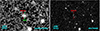 |
Fig. 1. Image of the galaxy plus blob in the SHARDS F551W17 filter (left panel) and in the HST/ACS F606W filter (right panel). In the HST/ACS filter the blob is not visible. |
The photometric redshift of SHARDS20018464 is z = 3.49 ± 0.06 (Barro et al. 2019; Arrabal Haro et al. 2020). At this redshift, the Lyα emission (at 1215.67 Å) moves to 5458.36 Å, that is within the SHARDS F551W17 filter range. The fact that SHARDS20018464 has his most-brilliant emission in this filter and that the blob is only visible in the same spectral range and just 3 pixels away from the galaxy position strongly suggests that the blob is linked to the parent galaxy.
3. Flux measurements
We ran SExtractor (Bertin & Arnouts 1996) to characterise the galaxy+blob detection in the SHARDS filter. In the header of the image we found the calibration constant, namely, 33.0785 mag in the AB system.
We used this calibration to estimate the AB magnitudes in the rest of our work and we also computed the surface-brightness (SB) zero point using the formula ZP = 33.0785 + 5 × log(0.254), where  is the pixel scale of the image. This ZP will be used for calibrating the surface brightness profile of the object. We report the values associated with the SExtractor detection in the corresponding section of Table 1. The AB magnitude of the object is 25.35 mag, estimated using the mag_auto parameter. SExtractor is not able to separate the galaxy from the blob, thus, we only used this measurement as a reference.
Properties of SHARDS20018464 and of its two components.
3.1. Galaxy and blob deconvolution
The main method adopted in this work for measuring the luminosity of the galaxy and the blob is to estimate the excess of light after removing a Sérsic profile. Since the blob and the galaxy have their centres apparently aligned on the CCD (same Y pixel coordinate), we used the centre of the galaxy (red circle in Fig. 2) as the starting point to analyse the four directions parallels to the axes of the image (from the centre to the top, bottom, left, and right). In this way, we have three directions where we can assume that only the galaxy contributes and one where the blob is dominant.
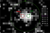 |
Fig. 2. Blob and its host galaxy. The large green circle represents a region of 2 |

The results are shown in Fig. 3. Black dotted lines are the three directions where only the galaxy is dominant and indeed they follow a quite similar profile. In blue, we overplotted the mean of these three lines (with the relative error bars, given by the dispersion of the data) and the green solid line is a Sérsic profile with Sérsic index n = 1, effective radius re = 0.38, and effective intensity Ie = 7.8. We note that this profile is not a fit, since the number of available points is too small. However, it follows quite well the blue line and it remains within the errors, so we can consider it as a reasonable representation of the profile of the galaxy.
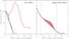 |
Fig. 3. Results from our main method (subtraction of a Sérsic profile to the SB profile of the galaxy, left panel) and from the ellipse-fitting method (right panel). Left panel: radial profiles of the galaxy in the three directions where the blob is not present (black dotted lines). The mean profile is represented with the blue dashed line (with corresponding uncertainties) and the Sérsic profile that we choose to represent the profile is shown with the green solid line. The red solid line represents the profile of the blob. Right panel: radial dependency of the intensity of the ellipses fitted with the IRAF task ellipse. The peak centred at about sma = 4 corresponds to the region of the blob. The red dashed line is connecting two points of the profile: the internal one is where there is an abrupt change in the slope of the profile, whereas the external point is the last point above the zero level. These two points are indicated by the two vertical lines. The coral area represent the difference between the profile and the red dashed line. |
The red solid line represents the profile in the direction of the blob. It can be seen that in this kind of decomposition, the blob starts dominating already in the second pixel and its flux peaks at about the third pixel ( or ∼5.7 kpc).
We then estimated the luminosity of the blob computing the difference between the area under the red solid line and the area of the green solid line that we adopted as the model of the galaxy in this approximation. This is an upper limit to our estimates, since we assume that the blob is the strongest contributor to the emission. However, it is probably the most precise description of what we are observing, since the model of the galaxy is coherent in three out of four directions and we can thus expect that in the fourth direction its contribution remains the same.
The luminosity of the blob is 1.04 × 1043, that of the galaxy is 2.87 × 1042, and the total flux is 1.33 × 1043. All the results are reported in Table 1. We can also estimate the flux with other two methods to confirm the robustness of the results and to give a lower limit to the Lyα emission from the blob. In the first comparison method, we identified the two peaks with the maximum emission in the F551W17 filter. These peaks correspond, in our interpretation, to the centre of the galaxy and the blob, respectively (as in the main method). In Fig. 2, both centres are visible along the same row, with the blob being on the right and highlighted with a small green circle, whereas the galaxy is on the left, highlighted with the small red circle.
We then focus our attention on a tiny region of nine rows around the position where the peaks of the blob and its host galaxy are found (indicated with arrows in the right side of Fig. 2). Each of these rows is represented with the corresponding intensity plot in Fig. 4. The intensity of these nine lines are shown individually, with the violet one representing the row that includes the two peaks (line 4). Moreover, we show in red the intensity profile of the collapsed lines (e.g. the pixel-to-pixel sum of the nine lines). We then fit a double Gaussian’s function to this red row (galaxy+blob), in order to estimate the contribution of each component. Using this method, we estimated a total magnitude of 25.59 AB and a total luminosity of 3.34 × 1042 erg s−1. To do so, we computed the flux in ADUs for the sum of all the pixels of the nine lines and then applied the calibration constant to get the AB magnitude and the flux.
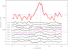 |
Fig. 4. Intensity plots of the nine rows around the peaks of the blob and its host galaxy. The pixels row containing the emission peaks of the blob and the galaxy companion is highlighted in violet, whereas in red we show the combination of all the nine lines fitted with a double Gaussian function (blue dotted line). The vertical axis is in arbitrary unit since, for sake of clarity, we add a vertical offset of 40 ADU to every individual row. Moreover, we also added 450 ADUs to the counts of the red solid line. |
We can also estimate the flux in ADUs (and magnitudes) for the Gaussian of the blob and the galaxy separately in the following way. First, we fit a single Gaussian to the position of the blob (thus forcing the peak in a specific position; see the top panel of Fig. 5). We then removed this Gaussian from the profile and we fit another one to the residuals, which (in this case) represents the underlying galaxy (bottom panel of Fig. 5). For both Gaussians, we can estimate the ADU fluxes and the AB magnitudes of the two components as in the previous paragraph. The results are reported in Table 1.
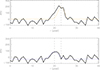 |
Fig. 5. Intensity plot of the combination of the 9 lines around the galaxy and blob. In the top panel, the black line is the same as the red line of Fig. 4) and the peak corresponding to the blob is fitted with a single Gaussian function. In the bottom panel, such Gaussian is removed from the profile and a different Gaussian function is fitted to the remaining signal, corresponding to the flux of the host galaxy. The vertical dashed lines are the same as in Fig. 4 and represent the peaks of the emission of the galaxy and the blob. |
The Lyα luminosities of the blob and the galaxy, according to this method and assuming that all the light in the F551W17 filter is due to the Lyα emission, are 2.34 × 1042 and 2.40 × 1042 erg s−1, respectively. The total luminosity is 3.34 × 1042 erg s−1, since in this approximation the object is slightly fainter than when compared to SExtractor results. This can be due to the different estimation of the sky level, since for the Gaussian fitted to the blob, it is assumed that the sky starts at zero ADUs, whereas it is probably fainter.
Another comparison method is based on the isophotes fitting of the galaxy using the IRAF1 task ellipse. The centre of the fit is the peak of the galaxy (e.g. the pixel highlighted with the small red circle in Fig. 2) and the ellipse fitting was performed using fixed semi-major axis progression, with step of 0.2 pixels. We did not mask the image, since there is no visible contamination from external sources and we needed to maximise the number of pixels available for the analysis. From ellipse, we obtained the intensity profile (shown in the right panel of Fig. 3) with the black thick solid line.
We then tried to perform the photometric decomposition of the galaxy using GASP2D (Méndez-Abreu et al. 2008), but we were not able to find a good fit; this is probably due to the fact that the code was written to work with large galaxies (more than 100 pixel in radius) and, in this case, the number of available pixels was too small ( < 10). For this reason, we constructed the line connecting two peculiar points of the profile, shown as a dashed-red line in the right panel of Fig. 3. The inner one is the point (at 1.3 pixel) at which the slope of the profile changes abruptly (e.g. as if the galaxy was dominated by a bulge in the inner part and a disc in the external regions). The external point is the last point of the ellipse fitting where the ellipse is fitted and not just a copy of the previous one (6.3 pixel). It is worth noting that this is just an approximation, with the goal being to establish a lower limit to the luminosity of the blob. Specifically, we are assuming that the larger fraction of the light has to be associated with the galaxy. As a consequence, the peak of the blob is diluted. Moreover, since the ellipse procedure is providing the radial profile of the entire ellipse, each point of the blob is also diluted in all the other points of the isophote, mostly dominated by the companion galaxy.
We estimated the flux of the blob as the difference between the area under the black thick curve and the one under the red dashed line in the selected region (e.g. included within the two vertical lines at 1.3 and 6.3 pixels in Fig. 3). In the same figure, we show this area in coral. The red dashed line represents our model of the galaxy in that region. The total magnitude of the galaxy (without the contribution of the blob) is obtained by adding the area under the red dashed line in the range 1.3 − 6.3 pixels to the area of the central region (e.g. the area under the black curve with radius smaller than 1.3 pixels). The result is a magnitude estimated between 0 and 6.3 pixels.
From the area of the blob, we estimated a magnitude of 26.35 mag, fainter than the previous estimation of 25.97 that we got with our main method. The flux of the blob is 1.65 × 1042 erg s−1 and, indeed, we stress that, with this method, we are giving a lower limit to the luminosity of the blob, assuming that most of the light is due to the companion galaxy. As a consequence, the magnitude of the galaxy is 24.90 mag with this method and the total one is 24.61 mag. The latter estimation is thus brighter than the SExtractor one.
3.2. Morphology and sizes
It is worth noticing that in the SHARDS filters the object has a very small angular size, so that its apparent size on the SHARDS image is dominated by the seeing. In our specific image, the seeing was computed with IRAF task imexam as 1 0, corresponding to 3.9 pixels. As shown in Fig. 3, the separation of the galaxy and blob peaks is only ∼3 pixels, just resolved under the seeing conditions. The pixel scale of our observations is 0
 254 per pixel, so that the separation is 0
 76. Since the object is found at z = 3.49, the physical scale is 7.478 kpc/″. Therefore, the physical separation between the galaxy and the blob is only 5.7 kpc.
3.3. Continuum
To properly estimate the continuum luminosity, we used the HST image available from the CANDELS program (Koekemoer et al. 2011). We used the HST/ACS F606W broadband filter, since its range is 4700–7000 Å, and, thus, it includes the F551W17 SHARDS filter. We ran SExtractor on the image (as we did for the SHARDS one) and repeated the same steps in order to estimate the luminosity of the galaxy in this band. The results are reported in Table 1. We also include the value of the continuum per unit wavelength at the filters centre (5809.26 Å, corresponding to 1293 Å rest-frame for the redshift of the object), in erg s−1 Å−1.
SExtractor also estimates the Kron radius of the galaxy, that is 5.79 pixels. The scale of the ACS camera is 0 05, thus the Kron radius of the galaxy in the ACS F606W broadband filter is 2.2 kpc. This size is about 50% of the size of the galaxy in the SHARDS filter, thus confirming that seeing is a dominant effect in those images. However, the blob is only visible in the narrower SHARDS filter, which reinforces the idea of it being a blob of emission produced by the Lyα photons in a very narrow wavelength range.
3.4. Lyα equivalent width
We measure the Lyα equivalent width (EW) associated with the different deconvolutions of the galaxy (continuum) and the blob (mostly Lyα emission), as well as directly combining the SHARDS F551W17 luminosity with the continuum level estimated from the HST/ACS F606W broadband filter. We considered the latter value (EW(Lyα) = 104 Å rest-frame) as the most reliable one, since it is independent of the model. We want to stress that the equivalent width so derived is completely consistent with the results of the deconvolution by the Sérsic profiles (EW(Lyα) = 111 Å rest-frame). These values are also consistent with the Lyα EW estimated for this source in Arrabal Haro et al. (2018), solely based on the SHARDS observations (126 Å). The derived EW(Lyα) and L(Lyα) values for all the methods are listed in Table 1.
4. Discussion and conclusions
We find the scenario that best describes the blob is the one that we present as our main method in this work, namely, the excess of light in the SB profile after removing a Sérsic model of the galaxy. In this section, we focus on a discussion of this result. However, we stress that it is compatible with the other two methods, which remain useful to assess the quality of the result and to provide a lower limit to the blob’s emission.
The morphology of this LAB is similar to several LAB encountered by Matsuda et al. (2011) in their survey of blobs at z ∼ 3. However, our blob is smaller in size, being at most 5 − 8 kpc versus the more than 100 kpc of all the blobs in their sample.
The host galaxy was modelled with a Sérsic profile with n = 1, meaning that this is a disc galaxy. This is in agreement with expectations from Kartaltepe et al. (2023), who found that 60% of galaxies at z = 3 are disc galaxies. The size of the galaxy is small, with a Kron radius of 2.2 kpc in the HST image. These values are in agreement with Lumbreras-Calle et al. (2019). In particular, these authors found that star-forming galaxies can be split into two classes, one with small Sérsic indexes and small effective radii and the other with large Sérsic indexes and large effective radii. The former are expected to be blue, whereas the latter are red. In a forthcoming work we will analyse the colour of the host galaxy for this object and for a larger sample of Lyα blob candidates; however, according to the size and n index, we expect that SHARDS20018464 should be a blue galaxy.
As shown in Fig. 2, the Lyα blob is clearly associated with a strong source of UV continuum, although each component peaks at a different location, not being co-spatial. We will first analyse whether the cluster of massive, potentially young stars that originates the UV continuum could also emit enough photo-ionising photons to produce the observed Lyα emission. As shown in Table 1, the global Lyα equivalent width of the system should be 111 Å (rest-frame). This value is perfectly consistent with the predictions for strong episodes of massive star formation, as shown by Rodríguez Espinosa et al. (2021). Synthesis models predict intrinsic values of EW(Lyα) around 100 Å for coeval starbursts at an age around 3 Myr, but they would be also consistent with an extended episode of star formation already in its equilibrium phase (after around 30 Myr) when the number of massive stars that are born balances the ones that finish their lifetime.
We want to stress that the observed values of EW(Lyα) should be considered just as a lower limit, since the Lyα photons are strongly affected by scattering and associated destruction by dust, so that their escape fraction is usually well below fesc, Lyα = 1.0. We have applied the semi-empirical calibration by Sobral & Matthee (2019) (fesc, Lyα = 0.0048 × EW(Lyα)±0.05) to derive an estimate of the Lyα escape fraction, resulting in fesc, Lyα ∼ 0.53 ± 0.05. This is a relatively high result for a Lyα emitting galaxy (Hayes et al. 2011). Correcting the observed Lyα emission by this escape fraction, we would get values of the intrinsic EW(Lyα) around 208 ± 20 Å, which would bring the age of the starbursts to ∼2.5 Myr for a coeval burst and around 4 Myr for a more extended episode. Such a large value of the intrinsic EW(Lyα) would be incompatible with the formation of massive stars for longer than around 5 Myr. Indeed, any value of fesc, Lyα ≲ 0.9 would lead to an intrinsic EW(Lyα) ≳ 125 Å, too large for a long-lasting star formation episode (Rodríguez Espinosa et al. 2021).
Synthesis models also allow us to estimate the strength of the star formation process that has originated this Lyα blob. Using the calibrations carried out by Otí-Floranes & Mas-Hesse (2010), we find that enough ionising photons would be emitted to yield the observed Lyα by a coeval star formation episode having transformed 1.2 × 10⁷ M⊙ of gas into stars, as well as by an extended episode at an average star formation rate of 2 M⊙/yr. We note that in both cases, this result would be normalised to a Salpeter initial mass function in the mass range of 2 − 120 M⊙. Assuming fesc, Lyα ∼ 0.5, these values would be 1.7 × 10⁷ M⊙ and 4.6 M⊙/yr, respectively.
Therefore, we conclude that a massive (1 − 2 × 10⁷ M⊙) super-cluster formed by young (around 2 − 4 Myr old) stars would be able to simultaneously produce the observed (rest-frame) UV continuum and produce enough ionising photons, as required to feed the observed Lyα luminosity.
IRAF is distributed by the National Optical Astronomy Observatories, which are operated by the Association of Universities for Research in Astronomy, Inc., under cooperative agreement with the National Science Foundation.
Acknowledgments
The authors thanks the anonymous referee for its useful comments that help clarifying the results of this paper. The authors also thanks Dr. Rosa Calvi for useful comments and discussion. This work is part of the collaboration ESTALLIDOS, supported by Spanish MICIU/AEI/10.13039/501100011033 grants PID2019-107408GB-C43 and PID2022-136598NB-C31, and by the Government of the Canary Islands through EU FEDER funding project PID2021010077. SZ and JMMH are also supported by the Spanish MICIU/AEI/10.13039/501100011033 grants PID2020119342GB-I00 and PID2023-147338NB-C21, respectively. Based on observations made with the Gran Telescopio Canarias (GTC), installed at the Spanish Observatorio del Roque de los Muchachos of the Instituto de Astrofísica de Canarias, on the island of La Palma. This work is based on data obtained with the SHARDS filter set, procured by Universidad Complutense de Madrid (UCM) through grant AYA2012-31277, and on observations made with the NASA/ESA Hubble Space Telescope obtained from the Space Telescope Science Institute, which is operated by the Association of Universities for Research in Astronomy, Inc., under NASA contract NAS 5–26555.
References
- Arrabal Haro, P., Rodríguez Espinosa, J. M., Muñoz-Tuñón, C., et al. 2018, MNRAS, 478, 3740 [NASA ADS] [CrossRef] [Google Scholar]
- Arrabal Haro, P., Rodríguez Espinosa, J. M., Muñoz-Tuñón, C., et al. 2020, MNRAS, 495, 1807 [NASA ADS] [CrossRef] [Google Scholar]
- Barro, G., Pérez-González, P. G., Cava, A., et al. 2019, ApJS, 243, 22 [NASA ADS] [CrossRef] [Google Scholar]
- Bennett, C. L., Larson, D., Weiland, J. L., & Hinshaw, G. 2014, ApJ, 794, 135 [Google Scholar]
- Bertin, E., & Arnouts, S. 1996, A&AS, 117, 393 [NASA ADS] [CrossRef] [EDP Sciences] [Google Scholar]
- Borisova, E., Cantalupo, S., Lilly, S. J., et al. 2016, ApJ, 831, 39 [Google Scholar]
- Brammer, G. B., van Dokkum, P. G., & Coppi, P. 2008, ApJ, 686, 1503 [Google Scholar]
- Bunker, A., Smith, J., Spinrad, H., Stern, D., & Warren, S. 2003, Ap&SS, 284, 357 [NASA ADS] [CrossRef] [Google Scholar]
- Caminha, G. B., Karman, W., Rosati, P., et al. 2016, A&A, 595, A100 [NASA ADS] [CrossRef] [EDP Sciences] [Google Scholar]
- Chapman, S. C., Lewis, G. F., Scott, D., et al. 2001, ApJ, 548, L17 [NASA ADS] [CrossRef] [Google Scholar]
- Christensen, L., Jahnke, K., Wisotzki, L., & Sánchez, S. F. 2006, A&A, 459, 717 [NASA ADS] [CrossRef] [EDP Sciences] [Google Scholar]
- Francis, P. J., & McDonnell, S. 2006, MNRAS, 370, 1372 [NASA ADS] [CrossRef] [Google Scholar]
- Fynbo, J. U., Møller, P., & Warren, S. J. 1999, MNRAS, 305, 849 [NASA ADS] [CrossRef] [Google Scholar]
- Geach, J. E., Alexander, D. M., Lehmer, B. D., et al. 2009, ApJ, 700, 1 [Google Scholar]
- Hayes, M., Schaerer, D., Östlin, G., et al. 2011, ApJ, 730, 8 [NASA ADS] [CrossRef] [Google Scholar]
- Heckman, T. M., Lehnert, M. D., Miley, G. K., & van Breugel, W. 1991, ApJ, 381, 373 [NASA ADS] [CrossRef] [Google Scholar]
- Herenz, E. C., Wisotzki, L., Roth, M., & Anders, F. 2015, A&A, 576, A115 [NASA ADS] [CrossRef] [EDP Sciences] [Google Scholar]
- Hu, E. M., & Cowie, L. L. 1987, ApJ, 317, L7 [NASA ADS] [CrossRef] [Google Scholar]
- Kartaltepe, J. S., Rose, C., Vanderhoof, B. N., et al. 2023, ApJ, 946, L15 [NASA ADS] [CrossRef] [Google Scholar]
- Kim, E., Yang, Y., Zabludoff, A., et al. 2020, ApJ, 894, 33 [CrossRef] [Google Scholar]
- Kimock, B., Narayanan, D., Smith, A., et al. 2021, ApJ, 909, 119 [NASA ADS] [CrossRef] [Google Scholar]
- Koekemoer, A. M., Faber, S. M., Ferguson, H. C., et al. 2011, ApJS, 197, 36 [NASA ADS] [CrossRef] [Google Scholar]
- Lehnert, M. D., & Becker, R. H. 1998, A&A, 332, 514 [NASA ADS] [Google Scholar]
- Lumbreras-Calle, A., Méndez-Abreu, J., & Muñoz-Tuñón, C. 2019, A&A, 632, A15 [NASA ADS] [CrossRef] [EDP Sciences] [Google Scholar]
- Matsuda, Y., Yamada, T., Hayashino, T., et al. 2004, AJ, 128, 569 [NASA ADS] [CrossRef] [Google Scholar]
- Matsuda, Y., Yamada, T., Hayashino, T., et al. 2011, MNRAS, 410, L13 [NASA ADS] [CrossRef] [Google Scholar]
- Méndez-Abreu, J., Aguerri, J. A. L., Corsini, E. M., & Simonneau, E. 2008, A&A, 478, 353 [NASA ADS] [CrossRef] [EDP Sciences] [Google Scholar]
- Miley, G., & De Breuck, C. 2008, A&ARv, 15, 67 [Google Scholar]
- Nilsson, K. K., Fynbo, J. P. U., Møller, P., Sommer-Larsen, J., & Ledoux, C. 2006, A&A, 452, L23 [NASA ADS] [CrossRef] [EDP Sciences] [Google Scholar]
- North, P. L., Courbin, F., Eigenbrod, A., & Chelouche, D. 2012, A&A, 542, A91 [NASA ADS] [CrossRef] [EDP Sciences] [Google Scholar]
- Ohyama, Y., Taniguchi, Y., Kawabata, K. S., et al. 2003, ApJ, 591, L9 [NASA ADS] [CrossRef] [Google Scholar]
- Otí-Floranes, H., & Mas-Hesse, J. M. 2010, A&A, 511, A61 [NASA ADS] [CrossRef] [EDP Sciences] [Google Scholar]
- Overzier, R. A., Nesvadba, N. P. H., Dijkstra, M., et al. 2013, ApJ, 771, 89 [NASA ADS] [CrossRef] [Google Scholar]
- Pérez-González, P. G., Cava, A., Barro, G., et al. 2013, ApJ, 762, 46 [Google Scholar]
- Prescott, M. K. M., Martin, C. L., & Dey, A. 2015, ApJ, 799, 62 [NASA ADS] [CrossRef] [Google Scholar]
- Ramakrishnan, V., Moon, B., Im, S. H., et al. 2023, ApJ, 951, 119 [NASA ADS] [CrossRef] [Google Scholar]
- Rodríguez Espinosa, J. M., Mas-Hesse, J. M., & Calvi, R. 2021, MNRAS, 503, 4242 [CrossRef] [Google Scholar]
- Scarlata, C., Colbert, J., Teplitz, H. I., et al. 2009, ApJ, 706, 1241 [NASA ADS] [CrossRef] [Google Scholar]
- Smith, D. J. B., & Jarvis, M. J. 2007, MNRAS, 378, L49 [NASA ADS] [Google Scholar]
- Sobral, D., & Matthee, J. 2019, A&A, 623, A157 [NASA ADS] [CrossRef] [EDP Sciences] [Google Scholar]
- Steidel, C. C., Adelberger, K. L., Shapley, A. E., et al. 2000, ApJ, 532, 170 [NASA ADS] [CrossRef] [Google Scholar]
- van Breugel, W., de Vries, W., Croft, S., et al. 2006, Astron. Nachr., 327, 175 [NASA ADS] [CrossRef] [Google Scholar]
- Villar-Martín, M., Vernet, J., di Serego Alighieri, S., et al. 2003, MNRAS, 346, 273 [CrossRef] [Google Scholar]
- Willott, C. J., Chet, S., Bergeron, J., & Hutchings, J. B. 2011, AJ, 142, 186 [CrossRef] [Google Scholar]
- Wilman, R. J., Gerssen, J., Bower, R. G., et al. 2005, Nature, 436, 227 [NASA ADS] [CrossRef] [Google Scholar]
- Yang, H., Wang, J., Zheng, Z.-Y., et al. 2014, ApJ, 784, 35 [NASA ADS] [CrossRef] [Google Scholar]
- Yang, Y., Zabludoff, A., Jahnke, K., et al. 2011, ApJ, 735, 87 [NASA ADS] [CrossRef] [Google Scholar]
All Tables
All Figures
|
Fig. 1. Image of the galaxy plus blob in the SHARDS F551W17 filter (left panel) and in the HST/ACS F606W filter (right panel). In the HST/ACS filter the blob is not visible. |
| In the text | |
|
Fig. 2. Blob and its host galaxy. The large green circle represents a region of 2 |
| In the text | |
|
Fig. 3. Results from our main method (subtraction of a Sérsic profile to the SB profile of the galaxy, left panel) and from the ellipse-fitting method (right panel). Left panel: radial profiles of the galaxy in the three directions where the blob is not present (black dotted lines). The mean profile is represented with the blue dashed line (with corresponding uncertainties) and the Sérsic profile that we choose to represent the profile is shown with the green solid line. The red solid line represents the profile of the blob. Right panel: radial dependency of the intensity of the ellipses fitted with the IRAF task ellipse. The peak centred at about sma = 4 corresponds to the region of the blob. The red dashed line is connecting two points of the profile: the internal one is where there is an abrupt change in the slope of the profile, whereas the external point is the last point above the zero level. These two points are indicated by the two vertical lines. The coral area represent the difference between the profile and the red dashed line. |
| In the text | |
|
Fig. 4. Intensity plots of the nine rows around the peaks of the blob and its host galaxy. The pixels row containing the emission peaks of the blob and the galaxy companion is highlighted in violet, whereas in red we show the combination of all the nine lines fitted with a double Gaussian function (blue dotted line). The vertical axis is in arbitrary unit since, for sake of clarity, we add a vertical offset of 40 ADU to every individual row. Moreover, we also added 450 ADUs to the counts of the red solid line. |
| In the text | |
|
Fig. 5. Intensity plot of the combination of the 9 lines around the galaxy and blob. In the top panel, the black line is the same as the red line of Fig. 4) and the peak corresponding to the blob is fitted with a single Gaussian function. In the bottom panel, such Gaussian is removed from the profile and a different Gaussian function is fitted to the remaining signal, corresponding to the flux of the host galaxy. The vertical dashed lines are the same as in Fig. 4 and represent the peaks of the emission of the galaxy and the blob. |
| In the text | |
Current usage metrics show cumulative count of Article Views (full-text article views including HTML views, PDF and ePub downloads, according to the available data) and Abstracts Views on Vision4Press platform.
Data correspond to usage on the plateform after 2015. The current usage metrics is available 48-96 hours after online publication and is updated daily on week days.
Initial download of the metrics may take a while.