| Issue |
A&A
Volume 683, March 2024
|
|
|---|---|---|
| Article Number | A241 | |
| Number of page(s) | 34 | |
| Section | Stellar atmospheres | |
| DOI | https://doi.org/10.1051/0004-6361/202346718 | |
| Published online | 28 March 2024 | |
Light curve and spectral modelling of the type IIb SN 2020acat
Evidence for a strong Ni bubble effect on the diffusion time
1
The Oskar Klein Centre, Department of Astronomy, AlbaNova, Stockholm University,
106 91
Stockholm, Sweden
e-mail: This email address is being protected from spambots. You need JavaScript enabled to view it.
2
Tuorla Observatory, Department of Physics and Astronomy,
20014
University of Turku, Finland
3
Finnish Centre for Astronomy with ESO (FINCA),
20014
University of Turku,
Finland
4
Cahill Center for Astrophysics, California Institute of Technology, MC 249-17,
1200 E California Boulevard,
Pasadena, CA
91125, USA
5
MIT-Kavli Institute for Astrophysics and Space Research,
77 Massachusetts Ave.,
Cambridge, MA
02139, USA
6
Facultad de Ciencias Astronómicas y Geofísicas, Universidad Nacional de La Plata,
Paseo del Bosque s/n,
B1900FWA
La Plata, Argentina
7
Instituto de Astrofísica de La Plata (IALP), CONICET,
B1900FWA,
La Plata, Argentina
8
Division of Physics, Mathematics, and Astronomy, California Institute of Technology,
Pasadena, CA
91125, USA
9
Astrophysical Research Institute Liverpool John Moores University,
Liverpool
L3 5RF, UK
10
Department of Astronomy, Kyoto University, Kitashirakawa-Oiwake-cho,
Sakyo-ku, Kyoto
606-8502, Japan
11
INAF – Osservatorio Astronomico di Padova,
Vicolo dell'Osservatorio 5,
35122
Padova, Italy
12
Department of Physics and Astronomy, Aarhus University,
Ny Munkegade 120,
8000
Aarhus C, Denmark
Received:
20
April
2023
Accepted:
3
August
2023
Abstract
We use the light-curve and spectral synthesis code JEKYLL to calculate a set of macroscopically mixed type IIb supernova (SN) models, which are compared to both previously published and new late-phase observations of SN 2020acat. The models differ in the initial mass, in the radial mixing and expansion of the radioactive material, and in the properties of the hydrogen envelope. The best match to the photospheric and nebular spectra and light curves of SN 2020acat is found for a model with an initial mass of 17 M⊙, strong radial mixing and expansion of the radioactive material, and a 0.1 M⊙ hydrogen envelope with a low hydrogen mass fraction of 0.27. The most interesting result is that strong expansion of the clumps containing radioactive material seems to be required to fit the observations of SN 2020acat both in the diffusion phase and in the nebular phase. These Ni bubbles are expected to expand due to heating from radioactive decays, but the degree of expansion is poorly constrained. Without strong expansion, there is a tension between the diffusion phase and the subsequent evolution, and models that fit the nebular phase produce a diffusion peak that is too broad. The diffusion-phase light curve is sensitive to the expansion of the Ni bubbles because the resulting Swiss-cheese-like geometry decreases the effective opacity and therefore the diffusion time. This effect has not been taken into account in previous light-curve modelling of stripped-envelope SNe, which may lead to a systematic underestimate of their ejecta masses. In addition to strong expansion, strong mixing of the radioactive material also seems to be required to fit the diffusion peak. It should be emphasized, however, that JEKYLL is limited to a geometry that is spherically symmetric on average, and large-scale asymmetries may also play a role. The relatively high initial mass found for the progenitor of SN 2020acat places it at the upper end of the mass distribution of type IIb SN progenitors, and a single-star origin cannot be excluded.
Key words: supernovae: individual: SN 2020acat / supernovae: general / radiative transfer
© The Authors 2024
 Open Access article, published by EDP Sciences, under the terms of the Creative Commons Attribution License (https://creativecommons.org/licenses/by/4.0), which permits unrestricted use, distribution, and reproduction in any medium, provided the original work is properly cited.
This article is published in open access under the Subscribe to Open model. This email address is being protected from spambots. You need JavaScript enabled to view it. to support open access publication.
1 Introduction
Ergon et al. (2018, hereafter E18,) and Ergon & Fransson (2022, herafter E22) presented and tested the light-curve and spectral synthesis code JEKYLL, and demonstrated its capability of modelling both the photospheric and nebular phase of supernovae (SNe). In particular, we demonstrated that both non-local thermodynamic equilibrium (NLTE) and the macroscopic mixing of the ejecta that occurs in the explosion need to be taken into account for the models to be realistic. As discussed in E22, the macroscopic mixing of the ejecta influences the SN in several ways: by preventing compositional mixing of the nuclear burning zones, which affects the strength of important lines in the nebular phase, and by expansion, of clumps containing radioactive material, which tends to decrease the effective opacity and therefore the diffusion time in the photospheric phase. The latter effect, which can be dramatic, has also been discussed by Dessart & Audit (2019) with respect to type IIP SNe, although in their case, the clumping was not directly linked to the expansion of the radioactive material. The magnitude of the effect depends on uncertain properties of the small-scale three-dimensional (3D) ejecta structure, such as the typical scale at which the fragmentation occurs in the explosion, and to which extent clumps containing radioactive material subsequently expand due to heating from radioactive decays. It is therefore of great interest to further constrain these properties. We note, however, that JEKYLL does not simulate the hydrodynamics giving rise to the macroscopically mixed ejecta, but uses a parametrised representation of these ejecta consisting of clumps of different composition, density, filling factor, and size (see Jerkstrand et al. 2011 and E22).
E22 applied JEKYLL to the type IIb SN 2011dh and showed that a macroscopically mixed SN model based on a progenitor with an initial mass of ~12 M⊙ reproduces the observed spectra and light curves of SN 2011dh well in both the photospheric and nebular phase. This is in line with previous work on this SN (see Maund et al. 2011; Bersten et al. 2011; Ergon et al. 2015; Jerkstrand et al. 2015) and underpins the emerging consensus that type IIb SNe mainly originate from relatively low-mass progenitors, which in turn suggests a binary origin. However, this conclusion is mainly based on approximate modelling, although for a few type IIb SNe (e.g. SNe 2011dh and 1993J), constraints were derived from both detailed NLTE modelling in the nebular phase (Jerkstrand et al. 2015) and progenitor detections (Aldering et al. 1994; Maund et al. 2011). It is therefore interesting to apply JEKYLL to another nearby well-observed type IIb SN to explore the constraints that can be obtained on the SN and progenitor parameters.
SN 2020acat was discovered on December 9, 2020 (Srivastav et al. 2020) and was classified as a type IIb by Pessi et al. (2020). Medler et al. (2022, hereafter M22) presented an extensive photometric and spectroscopic dataset, observational analysis, and approximate modelling of the SN. A complementing set of near-infrared (NIR) spectra was presented by Medler et al. (2023, hereafter M23). Here we present further late-time optical spectroscopy and photometry. Altogether, the data set for SN 2020acat is one of the best that have been obtained for type IIb SNe so far. Using the highly approximate (but classical) model of Arnett (1982) for the diffusion-phase light curve, M22 found an ejecta mass similar to that of SN 2011dh, whose origin from a relatively low-mass progenitor is well constrained. On the other hand, using a one-zone NLTE model for the nebular spectra, they found an oxygen mass of ~1 M⊙, indicating a progenitor of considerably higher initial mass than that of SN 2011dh. This tension1 motivates more detailed modelling, and it is interesting to determine whether the tension can be resolved by using JEKYLL, which self-consistently models both the photospheric and nebular phase using more elaborate physics.
The paper is organised as follows. In Sect. 2, we describe the observations of SN 2020acat and compare them to the observations of SN 2011dh, which provides a starting point for the modelling with JEKYLL. In Sect. 3, we briefly summarise the methods used by JEKYLL and describe our grid of type IIb SN models. In Sect. 4, we compare these models to the observations of SN 2020acat in order to constrain the SN and progenitor parameters. Finally, in Sect. 5 we summarise the paper.
New photometric observations of SN 2020acat.
2 Observations
2.1 Photometry
The bulk of the photometry for SN 2020acat was adopted from M22, and was obtained in the B, V, r, i, and z bands with the Nordic Optical Telescope (NOT), the Liverpool Telescope, the Asiago Copernico Telescope, the Palomar Samuel Oschin Telescope, the Mount Ekar Schmidt Telescope, and several telescopes that are part of the Las Cumbres Observatory Global Telescope (LCOGT; Brown et al. 2013), in the U and UVM2 bands with the Swift Observatory, and in the J, H, and K bands with the NOT and the New Technology Telescope (NTT). The reduction and calibration of these data are described in M22. In addition to this, we present new late-time optical photometry obtained at ~400 days with the Gemini South Telescope and the Faulkes Telescope North (part of the LCOGT). Complementary K-band photometry was also performed on the acquisition images for the NIR spectra obtained with the Keck Telescope (see Sect. 2.2). These additional photometric observations of SN 2020acat are listed in Table 1.
The Gemini South observations were obtained in the g and r bands at an epoch of 387 days using the Gemini Multi-Object Spectrograph (GMOS-S) instrument. The observations were reduced using the Gemini package included in IRAF, and point-spread function (PSF) photometry was performed with the DAOPHOT package. Instrumental magnitudes were calibrated to the standard AB system using 12 stars in the SN field to compute zero-point corrections relative to the Panoramic Survey Telescope and Rapid Response System (PanSTARRS) 1 catalogue.
The Faulkes Telescope North observations were obtained in the r band at an epoch of 404 days using the Spectral Camera as part of program NOAO2020B-012 (PI: De). The individual reduced images were retrieved from the on-line LCOGT archive, followed by stacking and photometric calibration against the PanSTARRS 1 catalogue. We subtracted the host galaxy light using archival PanSTARRS 1 images as templates, following the method described in De et al. (2020). The flux of the source was estimated by performing forced PSF photometry on the difference images.
The Keck K-band observations were obtained at epochs of 16, 77, 135, and 167 days using the NIRES instrument as part of the spectroscopic observations. The images were reduced and the photometry was performed and calibrated to the 2 Micron All Sky Survey (2MASS) system using the IRAF-based SNE pipeline (Ergon et al. 2014). For the calibration, a two-step procedure was used, where the magnitudes of the stars visible in the Keck images were first measured and calibrated to the 2MASS system using NIR images with a wider field of view obtained with the NOT.
Finally, in addition to what was done in M22, we also applied spectral corrections (S-corrections; see Stritzinger et al. 2002) to the photometry. In the nebular phase, these corrections can be substantial (for a discussion of this with respect SN 2011dh and details about the procedure, see Ergon et al. (2018) and references therein). Instrumental filter-response functions were constructed from filter and CCD data provided by the observatory or the manufacturer and extinction data for the site. S-corrections were then calculated based on the these instrumental response functions, the filter-response functions for the Johnson-Cousins (JC), Sloan Digital Sky Survey (SDSS), and 2MASS standard systems and the spectral evolution of SN 2020acat.
New spectral observations of SN 2020acat.
2.2 Spectra
The bulk of the spectra for SN 2020acat were adopted from M22 and M23, and were obtained with the NOT using the ALFOSC instrument, the Asiago Copernico Telescope, and the Keck Telescope using the NIRES instruments. In addition to this, we present new late-time spectra obtained with the Very Large Telescope (VLT) using the FORS2 and X-shooter instruments, the Gemini South Telescope using the GMOS-S instrument, and the Keck Telescope using the LRIS instrument. These additional spectral observations of SN 2020acat are listed in Table 2.
The VLT observations were obtained at an epoch of 106 days using the X-shooter instrument, and at an epoch of 204 days using the FORS2 instrument with grism 300 V. The X-shooter and FORS2 spectra were reduced and calibrated using ESOReflex (Freudling et al. 2013) following standard procedures, which include bias subtraction, flat-fielding, wavelength calibration, and flux calibration with a spectrophotometric standard star.
The Gemini South observations were obtained at an epoch of 387 days using the GMOS-S instrument with the R400 grating. The wavelength calibration was done using Cu-Ar lamps, and the flux calibration was done with a spectrophotometric standard star. The VLT FORS2 observations were obtained as part of the FORS+ Survey of Supernovae in Late Times program (FOSSIL; Kuncarayakti et al. in prep; see Kuncarayakti et al. 2022).
The Keck/LRIS observations were obtained at an epoch of 422 days. The data were reduced using the fully automated data-reduction pipeline LPipe (Perley 2019). An observation of G191-B2B taken on the same night was used for flux calibration.
Unfortunately, simultaneous NIR photometry to flux-calibrate the Keck NIR spectra was not originally obtained. Therefore, as mentioned in the previous section, we measured additional K-band photometry from the acquisition images, and otherwise relied on interpolations from the J- and H-band photometry obtained with NOT and NTT. However, after 115 days, no J- and H-band photometry is available, so in this case, we decided to extrapolate the J-band evolution using our optimal model for SN 2020acat and linearly interpolated between this and the measured K-band magnitudes. This should be kept in mind while examining the J- and H-band regions of the NIR spectra obtained after 115 days.
2.3 Distance, extinction, and explosion epoch
According to the NASA/IPAC Extragalactic Databse (NED), the host galaxy PGC037027 has a redshift of z = 0.00793, which, using a cosmology with H0 = 73.0 ± 5 km s−1 Mpc−1, Ωm = 0.27, and ΩΛ = 0.73, corresponds to a Hubble flow distance of 35.3 ± 4 Mpc (see M22 for a discussion of the error bar), corrected for the influence of the Virgo cluster, the Great Attractor, and the Shapley supercluster. This in turn corresponds to a distance modulus m – M = 32.74 ± 0.27 mag.
As in M22, we assumed that the extinction within the host galaxy is negligible, which is supported by the absence of host galaxy Na I D lines and the position of SN within the host galaxy. Based on this assumption, the total extinction is the same as the extinction within the Milky Way along the line of sight, which is E(B – V) = 0.021 mag, according to NED.
The constraints on the explosion epoch are good, and only two days lie between the last non-detection at MJD = 59190.61 and the first detection at MJD = 59192.65. In contrast to M22, who used a fit to the pseudo-bolometric light curve to determine the explosion epoch, we simply adopted the midpoint between the last non-detection and the first detection (MJD = 59191.63) as the explosion epoch.
2.4 Comparison to SN 2011 dh
Because SN 2011dh was modelled by JEKYLL in E22 and has both excellent data and well-constrained SN and progenitor parameters, it is of particular interest to compare the observations of SN 2020acat to this SN. The main purpose is to provide a starting point for the modelling of SN 2020acat with JEKYLL, but we also discuss some other topics.
2.4.1 Light curves
Figure 1 shows the optical, NIR, and pseudo-bolometric uBVriz light curves of SN 2020acat compared to SN 2011dh. In the figure, we also show cubic spline fits to the data, and for sparsely sampled bands, interpolations in colour. In general, the light curves are quite similar and show a rise to a bell-shaped maximum followed by a tail with a roughly linear decline that is characteristic for type IIb and other stripped-envelope (SE) SNe. The maximum is less pronounced and occurs later for redder bands, and the decline rate on the tail is initially lower for bluer bands, but increases subsequently. The maximum is shaped by diffusion of the energy deposited by the radioactive 56Ni synthe-sised in the SN explosion, and the tail, where the SN becomes optically thin, is shaped by the instant release of this energy. For SN 2011dh, an initial decline phase was also observed by PTF (Arcavi et al. 2011). This is seen in many type IIb SNe and is caused by the cooling of their low-mass hydrogen envelopes.
This phase is not observed in SN 2020acat, and because the first observation is from approximately one day, it has to be short. For a more detailed discussion of the light curves of SN 2011dh and type IIb SNe in general, see Ergon et al. (2014, Ergon et al. 2015) and E22.
However, there are also differences. SN 2020acat is more luminous than SN 2011dh, peaks earlier, and declines more slowly on the tail. This is further illustrated by Table 3, where we list the times and magnitudes of the peak as well as the tail decline rates for the pseudo-bolometric uBVriz light curves. We note that the tail decline rate is roughly similar in the beginning, and then increases for SN 2011dh at ~100 days and for SN 2020acat at ~150 days, after which it becomes roughly similar again. This is consistent with SN 2020acat becoming optically thin to the γ-rays later than SN 2011dh. In addition, Fig. 1 shows that on the rise to peak luminosity, SN 2020acat is significantly bluer than SN 2011dh, at least when we focus on the optical bands. The evolution in the ultraviolet (UV) is also quite different: It shows a continues decline in SN 2011dh, but a pronounced diffusion peak in SN 2020acat. This could be related to the much shorter cooling phase for SN 2020acat. Another clear difference is the evolution of the r band in the nebular phase, which is directly related to the evolution of the [O I] 6300, 6364 Å lines.
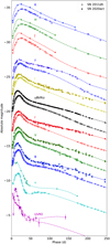 |
Fig. 1 Broadband and bolometric light curves until 250 days for SN 2020acat (filled circles) compared to SN 2011dh (empty squares). From bottom to top, we show the UVM2 (magenta), u (cyan), B (blue), V (green), r (red), ugBVriz pseudo-bolometric (black), i (yellow), z (blue), J (red), H (green), and K (blue) light curves. They are shifted for clarity by 6.0, 4.3, 2.0, 0.0, −2.3, −5.7, −7.7, −10.0, −13.0, −15.0, and −17.0 mags, respectively. |
2.4.2 Spectra
Figure 2 shows the optical and NIR spectral evolution of SN 2020acat compared to SN 2011dh. In this and all following figures, the spectra are time-interpolated as described in Ergon et al. (2014). If not otherwise stated, we only show interpolated spectra that have observed counterparts close in time. In general, the spectra are quite similar, showing the transition from a hydrogen-dominated to a helium-dominated spectrum, as is characteristic of type IIb SNe. Hα is initially the strongest line, but gradually disappears on the rise to the peak, whereas absorption in Hα and Hβ lines remains for a longer time. The helium lines appear on the rise to the peak and grow strong during the decline to the tail. The spectra also show lines from heavier elements, in particular, the Ca II 3934,3968 Å and Ca II 8498,8542,8662 Å lines (hereafter Ca II HK and Ca II NIR triplet), which are present throughout most of the evolution, and the forbidden [Ca II] 7291, 7323 Å and [O I] 6300, 6364 Å lines, which become the strongest lines during the nebular phase. For a more detailed discussion of the spectra of SN 2011dh and type IIb SNe in general, see Ergon et al. (2014, 2015), Jerkstrand et al. (2015), and E22.
However, there are also differences, and the lines of SN 2020acat are broader and the velocities are higher. This is further illustrated by Fig. 3, where we show the velocity evolution of the absorption minimum for the Hα and He I 7065 Å lines and the half-width at half-maximum (HWHM) velocity for the [O I] 6300,6364 Å lines for SNe 2020acat and 2011dh. The asymptotic Hα velocity, which likely corresponds to the interface between the helium core and hydrogen envelope (see Ergon et al. 2014, 2018) is ~ 12 000 km s−1 for SN 2020acat compared to ~11000 km s−1 for SN 2011dh. The He I 7065 Å velocity, which may be thought of as a representative for the helium envelope, is 38% higher (on average) for SN 2020acat, and the HWHM velocity of the [O I] 6300, 6364 Å line, which may be thought of as a representative for the carbon-oxygen core, is 20% higher (on average) for SN 2020acat. We also measured the velocity of the absorption minimum for the O I 7774 Å line and the HWHM velocity of the [Ca II] 7291, 7323 Å line, which are 30% and 33% higher (on average), respectively, for SN 2020acat.
In Fig. 4, we provide a closeup of the Hα and Hβ lines for SN 2020acat and SN 2011dh. Similar to the Ha line, the velocity of the Hβ line is higher in SN 2020acat, and the asymptotic velocity of the absorption minimum approaches 12 000 km s−1 for both lines. It also appears that the hydrogen signature is slightly stronger. In particular, these lines remain in absorption for a longer time in SN 2020acat. Whereas the Hα line disappears in absorption at ~80 days in SN2011dh, it remains in absorption at 100 days in SN 2020acat.
In Fig. 5, we provide a close-up of the He I 5876 Å and He I 1.083 μm lines between 10 and 150 days for SN 2020acat and SN 2011dh. Similar to the He I 7065 Å line, the velocities of these lines are higher in SN 2020acat, in particular at early times, and in particular for the He I 1.083 μm line. This line is also much stronger in SN 2020acat at early times. As discussed by M23, at late times, the He I 1.083 μm line (as well as the He I 2.058 μm line) attain a very distinct flat-topped shape for SN 2020acat, which is not seen in SN 2011dh.
It is also clear that the [O I] 6300, 6364 Å line, which is a tracer of the initial mass of the progenitor (see e.g Jerkstrand et al. 2015), is stronger in SN 2020acat. This is further illustrated in Fig. 6, where we show the [O I] 6300,6364 Å luminosity normalised with the pseudo-bolometric uBVriz luminosity and the luminosity of the 56Ni decay-chain for SN 2020acat and SN 2011dh. The line luminosity was measured with the same method as in Jerkstrand et al. (2015) to allow a comparison with Fig. 15 in that paper. Compared to the pseudo-bolometric uBVriz luminosity, the [O I] 6300, 6364 Å luminosity is 2.0 times higher (on average, after 150 days) for SN 2020acat, and compared to the 56Ni decay-chain luminosity, it is 3.8 times higher (on average, after 150 days) for SN 2020acat.
Finally, some other differences are also worth mentioning. First, the evolution of the Ca II HK and NIR triplet lines differ. Early on, these lines are absent in SN 2020acat, and later on, they are much weaker in absorption in SN 2020acat. Second, the quite strong [N II] 6548, 6583 Å lines emerging on the red shoulder of the [O I] 6300, 6364 Å lines towards ~300 days in SN 2011dh (see Jerkstrand et al. 2015) seem to be absent or at least much weaker in SN 2020acat.
Light-curve characteristics for the pseudo-bolometric uBVriz light curves of SN 2020acat and SN 2011dh measured from cubic spline fits.
2.5 Estimates of the SN parameters
We may attempt to use the comparison for an educated guess of how the SN parameters scale between SN 2011dh and SN 2020acat. Ergon (2015) fitted scaling relations for the SN parameters as a function of the observed quantities to a large grid of hydrodynamical SN models (see also Ergon et al. 2015). These were as follows:
 (1)
(1)
 (2)
(2)
 (3)
(3)
where tm, Lm, and vm are the time, luminosity, and photospheric velocity at the maximum. Measurements of tm and Lm for SN 2020acat and SN 2011dh are listed in Table 3. Measuring vm from Fig. 3 using the He I 7065 Å line as a proxy for the photosphere, Eqs. (1)–(3) give scale factors of 1.0, 2.1, and 1.7 for Μej, Eej and MNi, respectively, compared to SN 2011dh. Applying these scaling factors to the optimal model for SN 2011dh from E22, we obtain Mej=1.7 M⊙, Eej=1.4 B, and MNi=0.13 M⊙. This is qualitatively similar to the results in M22 using the Arnett model; as compared to SN 2011dh, the ejecta mass of SN 2020acat seems to be similar, whereas the kinetic energy of the ejecta and the mass of 56Ni seem to be much higher.
However, as is evident from Fig. 6, the strength of the [O I] 6300, 6364 Å lines points in another direction, suggesting a considerably higher oxygen mass in SN 2020acat, corresponding to a considerably higher ejecta mass (when we assume the progenitor to be an almost bare helium core). Assuming everything else to be equal, the [O I] 6300, 6364 Å luminosity normalised with the pseudo-bolometric luminosity would just scale with the fractional oxygen mass, which would then be 2.0 times higher. This corresponds to an ejecta mass that is about twice higher and an initial mass of ~17 M⊙ in the Woosley & Heger (2007) models. This is again qualitatively in line with the results by M22, who used one-zone NLTE modelling to find an oxygen mass of ~1 M⊙, corresponding to an initial mass of 16-17 M⊙.
Our educated guess for the SN parameters provides a starting point for the modelling with JEKYLL and a guideline for the SN models. Because of the inconclusive results for the initial mass, we treat this as a free parameter, whereas the velocities of the interfaces between the compositional layers and the mass of 56Ni were kept fixed based on the comparison. Instead, we took the opportunity to explore the parameters of the macroscopic mixing (which are not well constrained) and the properties of the hydrogen envelope.
3 Methods and models
The SN models presented in this work were calculated with the JEKYLL code, which is described in detail in E18, and E22. Here, we briefly repeat the general methods used in JEKYLL. The configuration of JEKYLL and the atomic data used are described in Appendices A and B, respectively.
Like in E22, the ejecta models are phenomenological models based on results from hydrodynamical modelling and the observed velocities of the ejecta. For the comparison with SN 2020acat, we present a set of models that differ in initial mass, radial mixing and expansion of the radioactive material, and in the mass and mass fraction of hydrogen in the hydrogen envelope.
3.1 JEKYLL
JEKYLL is a light-curve and spectral-synthesis code based on a Monte Carlo (MC) method for the time-dependent 3D radiative transfer developed by Lucy (2002, 2003, 2005), which was extended as described in E18,. To calculate the radiation field and the state of matter2, an iterative procedure is used, which is similar to an accelerated Λ-iteration (see the discussion in E18,). The statistical and thermal equilibrium equations are solved taking all relevant processes into account. In particular, this includes heating, excitation, and ionisation by non-thermal electrons calculated using the method by Kozma & Fransson (1992). In the inner region, where the matter and radiation field are assumed to be coupled, we use a diffusion solver to calculate the temperature.
JEKYLL also takes the macroscopic mixing of the ejecta into account by use of the virtual grid method (Jerkstrand et al. 2011), in which the fragmentation of the ejecta due to hydrodynamical instabilities is represented by spherical clumps characterized by their composition, density, size, and filling factor. The clumps are drawn based on their filling factor and geometrical cross section as the MC packets propagate through the ejecta, and they are virtual in the sense that they only exist as long as a MC packet propagates through them.
The main limitations in JEKYLL are the assumptions of homologous expansion, thermal and statistical equilibrium, and a spherically symmetric distribution of the matter. The latter is only assumed on large scales and on average, however, and small-scale asymmetries are taken into account through the virtual grid method. Another important limitation is the lack of a treatment of the ejecta chemistry (i.e. molecules and dust).
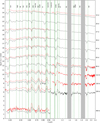 |
Fig. 2 Spectral evolution of SN 2020acat (red) compared to SN 2011dh (black). Spectra from ten logarithmically spaced epochs between 15 and 200 days and a single epoch at 400 days are shown. In addition, the rest wavelengths of the most important lines are shown as dashed green lines. |
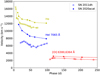 |
Fig. 3 Comparison of the evolution of the absorption minimum for the Hα (yellow) and He I 7065 Å (blue) lines and the HWHM of the [O I] 6300, 6364Å doublet for SN 2020acat (filled circles) and SN 2011dh (empty squares). |
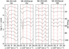 |
Fig. 4 Comparison of the evolution of the Hα and Hβ lines in SN 2020acat and SN 2011dh. Spectra from ten equally spaced epochs between 10 and 100 days are shown. Interpolated spectra that have no observed counterpart close in time are shown in grey. The inferred helium-hydrogen interface velocities of SNe 2011dh (11 000 km s−1) and 2020acat (12 000 km s−1) are shown as dashed red lines. |
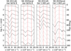 |
Fig. 5 Comparison of the evolution of the He I 5876 Å and He I 10 830 Å lines in SN 2020acat and SN 2011dh. Spectra from ten equally spaced epochs between 10 and 150 days are shown. Otherwise, this is the same as in Fig. 4. |
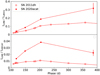 |
Fig. 6 Comparison of the evolution of the [O I] 6300, 6364 Å luminosity normalised with the pseudo-bolometric uBVriz luminosity (upper panel) and the 56Ni decay-chain luminosity (lower panel) for SN 2020acat (filled circles) and SN 2011dh (empty squares). |
3.2 Ejecta models
The ejecta models are based on SN models by Woosley & Heger (2007) for non-rotating single stars at solar metallicity with initial masses of 13, 15, 17, 19, and 21 M⊙, from which the helium core was carved out and the masses and abundances for the compositional layers were adopted. The stellar models were evolved to the verge of core-collapse and exploded with an energy of 1.2 B by Woosley & Heger (2007) using the 1D code Kepler. We note that the evolution depends on the assumed stellar parameters (no rotation and solar metallicity) as well as on the assumed progenitor system (single star). Moreover, the explosive nucleosynthesis and the amount of fallback onto the remnant depends on the assumed explosion energy (1.2 B) and on the simplified 1D explosion treatment in Kepler.
Following the approach in Jerkstrand et al. (2015), the carbon-oxygen core was assumed to have a constant (average) density, and the helium envelope to have the same (average) density profile as the best-fit model for SN 2011dh by Bersten et al. (2012). In addition, a low-mass hydrogen envelope based on models by Woosley et al. (1994) was attached. Based on the comparison with SN 2011dh (Sect. 2.4) and our previous successful model of this SN, the velocities of the interfaces between the carbon-oxygen core, the helium envelope, and the hydrogen envelope were set to 4200 and 12 000 km s−1, respectively, and the explosive nucleosynthesis was adjusted to match a 56Ni mass of 0.13 M⊙ (see below). We emphasise that the models are not self-consistent hydrodynamical models, but rather phenomenological models based on results from hydrodynamical simulations and the observed velocities and luminosity of SN 2020acat.
Based on the original onion-like compositional structure, we identify five compositional zones (O/C, O/Ne/Mg, O/Si/S, Si/S, and Ni/He) in the carbon-oxygen core and two compositional zones (He/N and He/C) in the helium envelope. The explosive nucleosynthesis was adjusted by scaling the mass of the Ni/He zone, whereas the Si/S and O/Si/S zones (which are also affected by the explosive nucleosynthesis) were left untouched. To mimic the mixing of the compositional zones in the explosion, three scenarios with different degrees of mixing of the radioactive material (weak, medium, and strong) were explored. In the weak-mixing scenario, the core is homogeneously mixed, but no core material is mixed into the envelope. In the medium-mixing scenario, 50% of the radioactive Ni/He material is mixed into the inner helium envelope, and in the strong-mixing scenario, 20% of this is mixed further into the outer helium envelope. The other material in the core is not mixed into the helium envelope in any of these scenarios, which is a simplification.
Given the mass-fractions of the compositional zones, the clumping geometry in our paramterisation is determined by the sizes (or masses) of the clumps and their filling factors (see E22). As discussed in Sect. 3.3, the constraints on the clumping geometry in type IIb SNe are rather weak, in particular with respect to the helium envelope. We assumed a clump mass of 2.8 × 10⁻⁵ M⊙ and explored three scenarios with different amounts of expansion (none, medium, and strong) of the radioactive material. In the medium-expansion scenario, we assumed a density contrast factor between the expanded and compressed material of 10 in the core and 5 in the helium envelope, and in the strong-expansion scenario, we assumed a density contrast factor of 60 in the core and 30 in the helium envelope. The main reason for keeping the clump mass fixed was to limit the computational cost (which is considerable). However, we note that the clump mass mainly affects the effective opacity because the decrease of this in a clumpy medium disappears when the clumps become optically thin (see E22). It is therefore somewhat degenerate with the expansion of the radioactive material, which further motivates our choice to keep one of these parameters fixed.
We also investigated the effect of the mass and mass fraction of hydrogen in the hydrogen envelope (which together determine the total mass of the hydrogen envelope), and explored three different masses (low, medium, and high), and two different mass fractions (low and medium). The medium scenario corresponds to a hydrogen mass of 0.027 M⊙ and XH=0.54. The low and high hydrogen-mass scenarios correspond to 0.0135 and 0.054 M⊙ and the low mass-fraction scenario corresponds to XH = 0.27. Our set of models thus differs in initial mass, radial mixing and expansion of the radioactive material, and in the mass and mass fraction of the hydrogen in the hydrogen envelope. All models are listed in Table 4, and a detailed description of each model is given in Appendix C.
In addition to this set of models, which is used to constrain the model parameters in Sect. 4.1, we calculated a few variants on the M17-s-m model for which we varied the metallicity and mass of 56Ni. We also calculated a model with a very strong expansion in the core (a contrast factor of 210). These models are listed in Table 5 and are referred to in Sect. 4.2 where we compare our optimal model with observations of SN 2020acat in detail.
Main set of ejecta models.
Additional set of ejecta models.
3.3 Macroscopic mixing in type IIb SNe
Our knowledge of the macroscopic mixing in type IIb SNe is limited, but there are some constraints, although they are generally weak. Some insights might also be gained from other types of SNe, not the least from SN 1987A.
For SN 1987A, a filling factor of 0.2 was estimated for the Ni/He material in the core by Kozma & Fransson (1998) using mid-IR (MIR) fine-structure Fe lines, and a filling factor of 0.1 was estimated for the oxygen-rich material in the core by Spyromilio & Pinto (1991) using the optical depth of the [O I] 6300, 6364 Å lines. Based on the core model for SN 1987A by Jerkstrand et al. (2011), this corresponds to an expansion factor of ~10 for the Ni/He material, a compression factor of ~5 for the oxygen-rich material, and a contrast factor of ~50. Based on a similar line of arguments, Jerkstrand et al. (2012) found a density contrast of ~30 between the Ni/He material and the oxygen-rich material in the core of the type IIP SN 2004et.
As a result of differences in the progenitor structure, this does not necessarily apply to type IIb SNe. In particular, the hydro-dynamical instabilities near the interface between the helium and hydrogen envelope are expected to be weaker in a type IIb SN. However, a high density contrast in the core is consistent with constraints on the filling factor of the oxygen-rich material (0.02 < Φ < 0.07) derived for SN 2011dh from small-scale variations in the [O I] 6300, 6364 Å and Mg I] 4571 Å line profiles (Ergon et al. 2015) and the optical depth of the [O I] 6300, 6364 Å lines (Jerkstrand et al. 2015). The cavities observed in the type IIb SN remnant Cas A also seem to indicate a considerable expansion of the radioactive material, even at high velocities (Milisavljevic & Fesen 2013, 2015). Overall, however, the constraints on the expansion of the radioactive material in type IIb SNe are weak, in particular with respect to the helium envelope.
For SN 1987A, the number of clumps in the oxygen-rich zones in the core was estimated to be ~2000 by Chugai (1994), who used a statistical model to analyse small-scale variations in the [O I] 6300, 6364 Å line profiles. Based on the core-model for SN 1987A by Jerkstrand et al. (2015), this corresponds to a clumps mass of ~10−3 M⊙. However, as for the contrast factor, this does not necessarily apply to type IIb SNe. Applying the Chugai (1994) model to SN 2011dh, Ergon et al. (2015) found a lower limit on the number of clumps in the O/Ne/Mg zone in the core of ~900 from small-scale variations in the [O I] 6300, 6364 Å and Mg I] 4571 Å line profiles. A similar limit was derived for SN 1993J by Matheson et al. (2000) using the same statistical model. Based on the core-model of SN 2011dh from Jerkstrand et al. (2015), the former limit corresponds to an upper limit on the clump mass of ~1.5 × 10⁻⁴ M⊙. To our best knowledge, there are no constraints on the sizes of the clumps in the helium envelope, and the constraints on the sizes of the clumps in type IIb SNe are weak overall.
The extent of the mixing in type IIb SNe is better constrained, and most light-curve modelling requires mixing of the He/Ni material far out in the helium envelope to reproduce the rise to peak luminosity (e.g. Ergon et al. 2015; Taddia et al. 2018). We note, however, that this modelling typically ignores the opacity increase that mixing of the Ni/He material gives rise to in the envelope. This limitation is absent from our JEKYLL simulations. Extensive mixing is also supported by explosion modelling (e.g. Wongwathanarat et al. 2017) and by the distribution of O-and Si-burning products in Cas A (e.g. Willingale et al. 2002). Finally, the assumption that the mixing is macroscopic is supported by both theoretical arguments (e.g. Fryxell et al. 1991) and by observations of SNe (e.g. Fransson & Chevalier 1989) and SNRs (e.g. Ennis et al. 2006). E22 discussed this issue in more detail and showed that microscopically mixed models of SN 2011dh give a very poor match to the [Ca II] 7291,7323 Å and [O I] 6300, 6364 Å lines in the nebular phase.
3.4 SN models
The ejecta models described in Sect. 3.2 were first (homologously) rescaled to one day. Based on an initial temperature profile, the SN models were then evolved with JEKYLL using 135 logarithmically spaced time steps to 501 days. The SN models were calculated using a frequency grid of 5000 logarithmically spaced intervals between 10 Å and 20,μm, and each model required ~25 000 central processing unit (CPU) hours. With 384 CPUs, this resulted in a computing time of ~3 days. The initial temperature profile was taken from a HYDE (Ergon et al. 2015) SN model for a 5 M⊙ bare helium core exploded with an energy of 1.1 B and ejecting 0.13 M⊙ of 56Ni. As this SN model was based on a bare helium core, the cooling of the thermal explosion energy, lasting for a few days in a model with a hydrogen envelope, was ignored. The subsequent evolution is powered by the continuous injection of radioactive decay energy, and the choice of an initial temperature profile is not critical, although it may have some effect on the early evolution.
We note that there is a switch in the JEKYLL setup at 100 days, when charge transfer and a more extended scheme for non-thermal excitation are turned on (see Appendix A). This can be visible as a slight shift in some of the model light curves. Moreover, some MC noise is present in the models, and in order to reduce this, gentle smoothing has been applied in some figures.
Finally, due to convergence difficulties in some low-density regions, the outer part of the hydrogen envelope was removed after 100 days, and the density was lowered in the expanded Fe/He clumps in the outer helium envelope after 50 days. Due to the extremely low optical depth in these regions at these epochs, this has no effect on the model spectra and light curves.
4 Comparisons to observations
We now proceed by comparing our JEKYLL models to the observations of SN 2020acat. In Sect. 4.1, we use the comparison to constrain the parameters of the model: the initial mass, the mixing and expansion of the radioactive material, and the mass and mass-fraction of hydrogen in the hydrogen-envelope. In Sect. 4.2, we compare the spectra and light curves of SN 2020acat in more detail to our optimal model, and discuss the remaining differences and their possible origin.
4.1 Constraining the model parameters
It is important to point out that because a full scan of parameter space is computationally not feasible, and because several limitations exist even in advanced SN models, we cannot hope for a perfect match. We should rather use a set of well-motivated key measures to search for a model that best fits the observations. To constrain the parameters of our models, we therefore applied five criteria: three criteria for the properties of the helium core, and two for the properties of the hydrogen envelope.
First, to constrain the properties of the helium core, that is, the initial mass and the mixing and expansion of the radioactive material, the optimal model should show the best overall match to the flux in the [O I] 6300, 6364 Å lines in the nebular phase and to the pseudo-bolometric light curve in both the diffusion and tail phase. These are all well-established criteria that have been used in a wide range of cases, and they are also well motivated from a physical point of view. In the nebular phase, the flux of the [O I] 6300, 6364 Å lines provides a measure of the oxygen mass, which is related to the helium core mass in our models. In the diffusion phase, the bolometric light curve provides a measure of the diffusion time for thermal radiation, whereas in the tail phase, it provides a measure of the optical depth to the γ-rays. These measures are both related to the ejecta mass, which in turn is related to the helium core mass in our models. In addition, the diffusion time is related to the expansion of the radioactive material (see E22), whereas the optical depth to the γ-rays is related to the mixing of this material. The capabilities of the JEKYLL code of modelling both the photospheric and nebular phase allow us to apply these three criteria in a self-consistent way based on highly sophisticated physics.
Second, to constrain the properties of the hydrogen envelope, the optimal model should show the best match to the hydrogen and helium lines in the photospheric phase. The strength and shape of these lines are related to the optical depths of these lines in the hydrogen envelope, which in turn are related to the mass of hydrogen and helium in the hydrogen envelope. As the hydrogen envelope in a type IIb has a relatively low mass and soon becomes more or less transparent, it does not have a significant impact on the other key quantities and can be constrained separately.
4.1.1 Helium core
To explore the properties of the helium core, we used the diffusion-phase pseudo-bolometric light curve, the tail phase pseudo-bolometric light curve and the nebular phase [O I] 6300, 6364 Å flux. First, the latter two were used two constrain the initial mass of the progenitor, and then the former was used to constrain the mixing and expansion of the radioactive material.
Figure 7 shows the evolution of the luminosity in the [O I] 6300, 6364 Å lines for SN 2020acat compared to models M13-m-s, M15-m-s, M17-m-s, M19-m-s, and M21-m-s, which all have medium mixing and strong expansion of the radioactive material and only differ in the initial mass. Clearly, in the 13 M⊙ model the luminosity is far too low at all epochs, whereas in the 21M⊙ model the luminosity is too high from ~150 days and onwards, and is far too high at ~400 days. It could be argued that later epochs are more reliable because the SN has then become more nebular and optical depth effects are weaker. In that case, both the 13 and 21 M⊙ model seem to be excluded, and the 17–19 M⊙ models match the observations best. We note that the JEKYLL models evolve more slowly overall than is observed for SN 2020acat. We return to this problem in Sect. 4.2.
In Fig. 8, we show the evolution of the luminosity in the [Ca II] 7291,7323 Å lines for SN 2020acat compared to the same models. Because these lines may overtake the cooling from the [O I] 6300, 6364 Å lines if calcium-rich material is mixed in some way with the oxygen-rich material (see E22), it is important to examine these lines as well. We note, however, that the [Ca II] 7291, 7323 Å lines mainly originate from the Si/S and O/Si/S zones, which are not adjusted to comply with the adopted 56Ni mass (see Sect. 3.2). This comparison therefore has to be taken with a grain of salt. Nevertheless, the 17-19 M⊙ models, which matched the evolution of the flux in the [O I] 6300, 6364 Å line best, also match the evolution of the flux in the [Ca II] 7291, 7323 Å lines reasonably well, which is assuring.
Figure 9 shows the pseudo-bolometric uBVriz light curve for SN 2020acat compared to models M13-m-s, M15-m-s, M17-m-s, M19-m-s, and M21-m-s, which all have medium mixing and strong expansion of the radioactive material, and only differ in the initial mass. During the diffusion phase, the model light curves are fairly similar, but during the tail phase, they diverge progressively. Compared to SN 2020acat, the luminosity of the 13 M⊙ model is too low and declines too fast, whereas the luminosity of the 21 M⊙ model is too high and declines too slowly.
This indicates that the optical depth to the γ-rays in the 13 and 21 M⊙ models is too low and too high, respectively. The best agreement with SN 2020acat in the tail phase is shown by the 15-17 M⊙ models. The similarity of the models in the diffusion phase may be surprising because of the quite large difference in ejecta mass, but in our models, the early evolution is largely determined by the helium envelope, which is not that different in the models. The mass of the helium envelope increases only slowly with initial mass, and the interface velocities are fixed by observations. We note that the tail luminosity and decline rate also depend on the mixing of the radioactive material, and high-mass models with extreme mixing and low-mass models with weak mixing may fit the tail better than the medium-mixing models shown here. The tail-phase comparison is therefore not conclusive in itself. However, in combination with the evolution of the flux in the [O I] 6300, 6364 Å lines, the 13 and 21 M⊙ models seem to be excluded, and the 17 M⊙ model matches best overall. The diffusion phase does not provide any useful constraints on the initial mass, but we used it instead to constrain the mixing and expansion of the radioactive material.
Figure 10 shows the pseudo-bolometric uBVriz light curve for SN 2020acat compared to models M17-m-n, M17-m-m, and M17-m-s, which all have an initial mass of 17 M⊙ and only differ in the expansion of the radioactive material. In contrast to the previous case, the tail-phase light curves are similar, whereas the diffusion phase light curves differ. The diffusion peak is clearly too broad for the models without or with only a mild expansion of the radioactive material, whereas the model with strong expansion of the radioactive material gives a much better fit. The reason for the differences in the diffusion phase light curve is that the expansion of the radioactive material decreases the effective opacity of the ejecta. This small-scale 3D effect is discussed in detail in E22 (see also Dessart & Audit 2019 for a discussion of this effect on type IIP SN light curves).
Figures 11 and 12 show the pseudo-bolometric uBVriz light curve for SN 2020acat compared to models with an initial mass of 17 M⊙ that only differ in the mixing of the radioactive material. In Fig. 11, we show models M17-w-n, M17-m-n, and M17-s-n, which have no expansion of the radioactive material, and in Fig. 12 we show models M17-w-s, M17-m-s, and M17-s-s, which have strong expansion of the radioactive material. Clearly, the diffusion peaks of the models with no expansion of the radioactive material are too broad, regardless of the mixing of this material. If the radioactive material is strongly expanded, the width of the diffusion peak becomes narrower and agrees better with the observations, and the best agreement is achieved with strong mixing of this material. With only weak mixing of the material, the peak becomes far too broad, which means that both strong mixing and strong expansion of the radioactive material seem to be required to fit the diffusion peak of SN 2020acat. We note that the peak luminosity is not fully reproduced by any of the models, and it is 15–20% fainter than for SN 2020acat. We return to this issue in Sect. 4.2. Moreover, the tail luminosity is too bright for the weakly mixed models. Although the match to the tail could be improved for these models by lowering the mass of 56Ni, this would give an even worse fit to the diffusion phase because it roughly corresponds to a scaling of the light curve.
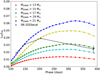 |
Fig. 7 Evolution of the luminosity in the [O I] 6300, 6364 Å lines normalised with the 56Ni decay luminosity for SN 2020acat (black crosses) and the JEKYLL models with strong expansion and medium mixing of the radioactive material and initial masses of 13 M⊙ (red), 15 M⊙ (cyan), 17 M⊙ (green), 19 M⊙ (yellow), and 21 M⊙ (blue). |
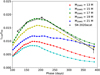 |
Fig. 8 Evolution of the luminosity in the [Ca II] 7291, 7323 Å lines normalised with 56Ni decay luminosity for SN 2020acat (black crosses) and the JEKYLL models with strong expansion and medium mixing of the radioactive material and initial masses of 13 M⊙ (red), 15 M⊙ (cyan), 17 M⊙ (green), 19 M⊙ (yellow), and 21 M⊙ (blue). |
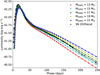 |
Fig. 9 Pseudo-bolometric uBVriz light curves until 250 days for SN 2020acat and JEKYLL models with strong expansion and medium mixing of the radioactive material and initial masses of 13 M⊙ (red), 15 M⊙ (cyan), 17 M⊙ (green), 19 M⊙ (yellow), and 21 M⊙ (blue). |
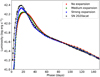 |
Fig. 10 Pseudo-bolometric uBVriz light curves until 150 days for SN 2020acat and JEKYLL models with an initial mass of 17 M⊙, medium mixing, and no, medium, and strong expansion of the radioactive material. |
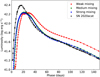 |
Fig. 11 Pseudo-bolometric uBVriz light curves until 150 days for SN 2020acat and JEKYLL models with an initial mass of 17 M⊙, no expansion, and weak, medium, and strong mixing of the radioactive material. |
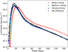 |
Fig. 12 Pseudo-bolometric uBVriz light curves until 150 days for SN 2020acat and JEKYLL models with an initial mass of 17 M⊙, strong expansion, and weak, medium, and strong mixing of the radioactive material. |
4.1.2 Hydrogen envelope
To explore the properties of the hydrogen envelope, we used the hydrogen and helium lines, where we first used the former to constrain the mass of hydrogen, and then the latter to constrain the mass fraction of hydrogen. For a given mass of hydrogen, this is inversely proportional to the total mass of the hydrogen envelope.
Figure 13 shows the evolution of the Ha and Hβ lines for SN 2020acat compared to models M17-s-s-H-low, M17-s-s, and M17-s-s-H-high, which only differ in the mass of hydrogen in the envelope. In the model with a high hydrogen mass (MH = 0.054 M⊙) the Ha and Hβ absorption becomes too strong towards 100 days, and in the model with a low hydrogen mass (MH =0.0135 M⊙) the absorption in these lines is too weak and appears at too low velocities. On the other hand, both the Ha and Hβ lines are reasonably well reproduced in the model with a medium hydrogen mass (MH=0.027 M⊙), and this model gives the best overall fit to the evolution of these lines.
Figure 14 shows the evolution of the He I 5876 Å and He I 1.083 μm lines for SN 2020acat compared to models M17-m-s, M17-s-s, and M17-s-s-XH-low, which all have a medium hydrogen mass and differ in the mass-fraction of hydrogen and the mixing of the radioactive material. Clearly, the match is worse for the models with a high hydrogen mass-fraction (XH = 0.54) than for the model with a low hydrogen mass-fraction (XH = 0.27), although a stronger mixing of the radioactive material improves the match somewhat due to non-thermal excitation and ionisation. In particular, the absorption in the He I 1.083 μm line is too weak at velocities above the interface between the helium and hydrogen envelope. The model with strong mixing and a low hydrogen mass-fraction gives the best match overall to the evolution of the He I 5876 Å and He I 1.083 μm lines.
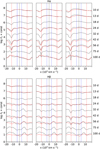 |
Fig. 13 Evolution of the Hα (upper panel) and Hβ (lower panel) lines for SN 2020acat (red) and the JEKYLL models (black) with an initial mass of 17 M⊙, strong mixing and strong expansion of the radioactive material, and a mass of hydrogen in the envelope of 0.0135 (left), 0.027 (middle), and 0.054 (right) M⊙. Spectra from nine logarithmically spaced epochs are shown, and the model C/O-He (blue) and He-H (red) interface velocities are indicated with dashed lines. |
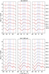 |
Fig. 14 Evolution of the He I 5876 Å (upper panel) and He I 1.083 μm (lower panel) lines for SN 2020acat (red) and the JEKYLL models (black) with an initial mass of 17 M⊙, strong expansion of the radioactive material, medium mixing plus XH =0.54 (left), strong mixing plus XH = 0.54 (middle), and strong mixing plus XH = 0.27 (right). The figure is otherwise the same as Fig. 13. |
4.1.3 Summary and discussion
In summary, the optimal model has an initial mass of 17 M⊙, strong mixing and strong expansion of the radioactive material, and a 0.1 M⊙ hydrogen envelope with XH = 0.27. In Sect. 4.2 we study this model in more detail, compare it with the observations of SN 2020acat, and discuss similarities as well as remaining differences and their possible origin. First, however, we discuss the main properties derived for our optimal model.
The most interesting result is perhaps the strong expansion of the radioactive material that seems to be required, and the accompanying strong effect of that on the diffusion phase light curve. As discussed in detail in E22, the expansion of the Ni/He clumps creates a density contrast between these and other clumps, which affects the radiative transfer and leads to a decrease in the effective opacity. This can be imagined as a Swiss-cheese-like geometry, in which the photons diffuse faster through the low-density Ni bubbles. The effect is strongest in the limit of optically thick clumps, and it disappears in the limit of optically thin clumps. As derived in E22, the decrease in the effective opacity in the limit of optically thick clumps is roughly given by the product of the (volume) expansion and filling factors for the Ni/He clumps.
This is illustrated by Fig. 15, where we show the (average) effective Rosseland mean opacity in the inner helium envelope for the model with strong expansion (M-17-s-m) and the corresponding limits for optically thick and thin clumps. Initially, the effective opacity follows the thick limit, which is a factor of ~5 below the thin limit and then gradually approaches the thin limit towards ~60 days, where the radiative transfer effect disappears. However, we also show in Fig. 15 the model without expansion (M17-n-m). Compared to that model, the effective opacity remains lower even after ~60 days. This is due to a density-driven recombination effect that was discussed in more detail by E22 and by Dessart et al. (2018). The radiative transfer and recombination effects are complementary, but the radiative transfer effect is stronger and dominates during the diffusion phase.
We point out, however, that we cannot rule out that physics outside the limitations of JEKYLL (see Sect. 3.1) may cause a similar effect on the diffusion phase light curve as the expansion of the Ni bubbles. Early-time CSM interaction seems unlikely because there are no signs of this in the spectra and because the mass-loss rate estimated from radio observations (Poonam et al. in prep.) is more similar to SN 2011dh than to interacting type IIb SNe as 1993J. Large-scale asymmetries are harder to rule out, and they may or may not give rise to a similar effect on the diffusion phase light curve. We discuss this issue further below. We note that the degree of expansion of the radioactive material is somewhat degenerate with the assumed clumps size (see Sect. 3.3), and larger clumps would require less expansion of this material to achieve the same effect on the light curve.
If the magnitude of the effect in our model of SN 2020acat were typical for type IIb and other SE SNe, it would have important implications for the entire literature of 1D light-curve modelling of these SNe. This applies to both simple (e.g Cano 2013; Lyman et al. 2016; Prentice et al. 2016) and more advanced (e.g Ergon et al. 2015; Taddia et al. 2018) 1D models because none of them take the effect of the Ni bubbles on the effective opacity into account. Depending somewhat on which weight is given to the diffusion-phase light curve, the ejecta masses derived from this modelling could be systematically and quite strongly underestimated.
Ignoring the effect may give rise to a tension between quantities derived from the diffusion and tail phases, similar to what we find for SN 2020acat. Interestingly, a tension like this has been reported by Wheeler et al. (2015) for a literature sample of SE SNe, although this tension may arise at least partly from other simplifications in their methods (see Nagy 2022). A tension like this has also been reported for several type Ic broad-line (BL) SNe. For SN 1998bw, Dessart et al. (2017) found that the tail phase required much more massive ejecta than the diffusion phase. Maeda et al. (2003) proposed that this could be explained by large-scale asymmetries in a jet-driven explosion and introduced a simple two-component ejecta model (see also Valenti et al. 2008 for a similar model). In this model, the low-density jet component, which is assumed to contain most of the Ni/He material, gives rise to a fast and luminous diffusion peak, whereas the high-density disk component, which is assumed to contain most of the oxygen-rich material, gives rise to the tail. While this ejecta geometry is not entirely far-fetched in the case of a Typ Ic-BL SN, which are thought to originate from a fast-rotating progenitor star, it makes less sense in the case of a type IIb SN.
To explain the early light curve of SN 1998bw, Höflich et al. (1999) proposed an oblate ejecta geometry. Oblate or prolate ejecta geometries depend on the viewing angle and may boost or suppress the luminosity during the diffusion phase due to the projected area of the photosphere (see also Kromer & Sim 2009 for a prolate type Ia toy model). This effect seems more plausible in the case of type IIb SNe, and would give rise to another form of tension between the diffusion and the tail phases that would be more related to the mass of 56Ni than the ejecta mass. Direct observational evidence for large-scale asymmetries in the ejecta of SNe can be searched for using polarimetry. Although no polarimetry was obtained for SN 2020acat, polarimetry have been obtained for several other type IIb SNe. The results show a continuum polarisation of ~0.5% during the helium-dominated phase for most objects (Mauerhan et al. 2015), which might be interpreted as moderately aspherical ejecta. This interpretation is not clear, however, because clumpy ejecta may also contribute to the continuum polarisation. Explosion models (Wongwathanarat et al. 2017) indicate that asymmetries arise on a wide range of scales in type IIb SNe, and although our results does not disprove that large-scale asymmetries affect their light curves, they do prove that small- and medium-scale asymmetries may also have a strong effect.
The strong mixing of the radioactive material required to fit the early light curve is in line with results from hydrodynamical modelling of type IIb SNe (e.g. Bersten et al. 2012; Ergon et al. 2015; Taddia et al. 2018). We note, however, that in our models strong expansion of this material is also required to reduce the effective opacity in the layers into which the material is mixed. This is likely related to the fact that in our models, the mixing of the radioactive material has an opposite effect and increases the opacity, both through the higher line-opacity of this material and through non-thermal ionisation. Strong mixing of the radioactive material is also in line with results from type IIb explosion models (Wongwathanarat et al. 2017) and observations of the type IIb SN remnant Cas A (e.g. Willingale et al. 2002).
The relatively high initial mass of ~17 M⊙ we derived places SN 2020acat at the upper end of the mass distribution for type IIb SNe. Jerkstrand et al. (2015) estimated initial masses well below 17 M⊙ for the progenitors of SNe 2008ax, 2011dh, and 1993J using modelling of their nebular spectra, which for the latter two is supported by stellar evolutionary analysis of pre-explosion imaging of the progenitors (Aldering et al. 1994; Maund et al. 2011). Ergon (2015) found that 56% of the type IIb progenitors have an initial mass lower than 15 M⊙ and 75% have an initial mass lower than 20 M⊙ using hydrodynamical light-curve modelling. The simplified treatment of the opacity and the 1D limitation (preventing the effect of the Ni bubbles on the diffusion time) makes this result uncertain, however. The relatively high initial mass we found for SN 2020acat also makes a singlestar origin more plausible. This is in contrast to SN 2011dh, for which a single-star origin seems to be excluded.
The low mass-fraction of hydrogen in the envelope we derived is more in line with a binary origin, however, because a low mass-fraction may naturally arise in a binary system during mass transfer onto the companion star (Yoon et al. 2010). The low mass-fraction of hydrogen in the envelope is also in line with the short cooling phase that SN 2020acat seems to have experienced (<1 day) because this tends to result in smaller progenitor radii. The extent of the cooling phase depends on several factors, however, and hydrodynamical modelling is needed to shed more light on this issue.
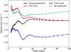 |
Fig. 15 Evolution of the (mass-averaged) effective Rosseland mean opacity in the inner helium envelope for the model with strong expansion (black) and the corresponding effective Rosseland mean opacity in the limits of optically thick (blue) and thin (red) clumps. In addition, we show the evolution of the effective Rosseland mean opacity for the model without expansion (cyan). |
4.2 Detailed comparison to SN 2020acat
In Sect. 4.1, we constrained the model parameters by comparing some key observables for SN 2020acat to our model grid, and we determined an optimal model (M17-s-s-XH-low) with an initial mass of 17 M⊙, strong mixing and expansion of the radioactive material, and a 0.1 M⊙ hydrogen envelope with XH = 0.27. We study this model in more detail here and compare the spectra and light curves in more detail to SN 2020acat. In addition, it is interesting to compare our model to the optimal model for SN 2011dh, which was first presented in Jerkstrand et al. (2015) and was then refined for the photospheric phase and discussed in detail in E22. This model has an initial mass of 12 M⊙, somewhat weaker mixing and expansion of the radioactive material, and a 0.1 M⊙ hydrogen envelope with XH=0.54. The models also differ in the mass of 56Ni and in the interface velocities, reflecting the lower luminosity and line velocities observed in SN 2011dh.
In Fig. 16, we show the evolution of the temperature, electron fraction, and radioactive energy deposition in the carbon-oxygen core, the inner and outer helium envelope, and the hydrogen envelope (averaged over the spatial cells and compositional zones)3, as well as the evolution of the photosphere for the optimal model of SN 2020acat, and in Figs. 17 and 18, we show the spectral evolution in the optical and NIR and the light curves in the UV, optical, and NIR for the optimal model compared to the observed evolution of SN 2020acat. In addition, in Figs. D.1–D.7, we show the contributions to the spectral evolution of the optimal model from the different spatial layers, compositional zones, and radiative processes giving rise to the emission. We note that there might be a slight shift in some quantities at 100 days when charge-transfer is turned on (see Appendix A).
The evolution of the model for SN 2020acat is qualitatively similar to that of the model for SN 2011dh (see E22, Figs. 2–4). This is expected because they are both type IIb SN models, although with different SN parameters. Initially (5 days), the photosphere is located in the inner part of the hydrogen envelope, which is relatively cool and recombined, whereas the core is hot and highly ionised. The emission mainly originates from the hydrogen envelope, and the hydrogen signature is strong with lines from the Balmer and Paschen series, mainly seen in emission. However, in contrast to the SN 2011dh model, the helium lines are already on the rise due to the stronger mixing of the radioactive material. After ~15 days, the photosphere begins to recede into the helium envelope, the emission from therein increases, and the helium lines continues to grow until they dominate the spectrum at ~40 days. The emission from the hydrogen line fades away on a similar timescale (although Hα and Hβ remain in absorption) and completes the transition from a hydrogen- to a helium-dominated spectrum.
Between ~40 days and ~60 days, the photosphere recedes through the inner parts of the helium envelope and thereafter through the carbon-oxygen core until it disappears at ~120 days, when the SN becomes nebular. During this period, emission from the carbon-oxygen core becomes stronger, and at ~120 days, it dominates redward of the B-band. As a consequence, emission from heavier elements that are abundant in the core increases, in particular after ~120 days, when the characteristic [O I] 6300, 6364 Å and [Ca II] 7291,7323 Å lines appear. During the nebular phase, this trend continues while the temperature, electron fraction, and energy deposition in the core decrease slowly. At 400 days, emission from the carbon-oxygen core dominates the entire optical and NIR spectrum, and the [O I] 6300, 6364 Å and [Ca II] 7291, 7323 Å lines alone contribute about a quarter of the total luminosity.
The agreement between the model and the observations of SN 2020cat is reasonable overall, and the main differences between SNe 2020acat and 2011dh discussed in Sect. 2.4 are reflected in our models. The luminosity is higher, the diffusion peak occurs earlier and is bluer, the line velocities are higher, the tail declines more slowly, and the [O I] 6300, 6364 Å lines are stronger in the SN 2020acat model. However, there are also notable differences between our model and the observations of SN 2020acat. During the diffusion phase, the peak luminosity is not entirely reproduced by the model, and it is too low in all bands. In our models, the peak-to-tail ratio is sensitive to the mixing of the Ni/He material, and a better fit might be achieved by tweaking this parameter. The difference is more pronounced in the NIR than in the optical and even more so in the UV, where the UVM2 light curve is to faint by almost 2 mags. As shown in Fig. 19, the UVM2 light curve is very sensitive to the metallicity, and this is more so during the diffusion peak than on the tail, so that the discrepancy in the UVM2 light curve could indicate subsolar metallicity. However, the UVM2 light curve is also quite sensitive to the mass of the hydrogen envelope and the extinction (which was assumed to be zero in the host galaxy), which means that these factors may contribute as well.
On the tail, we see a growing excess in the NIR, in particular in the K band, which is even more evident in the spectral comparison. This excess is reminiscent of SN 2011dh, where the excess was attributed to dust. However, in the case of SN 2011dh, a strong excess was also seen in the MIR, which underpinned this explanation. After ~100 days, a quite strong discrepancy also develops in the B and V bands, which are too bright in the model. We did not find any satisfying explanation for this by varying the parameters in our models, which indicates that the discrepancy originates from some process that is absent in our models. One such process is the formation of dust in the ejecta, which might absorb more strongly at bluer wavelengths. Another possible explanation is large-scale asymmetries in the ejecta because the SN is still optically thick in this wavelength region at ~200 days. This explanation is consistent with the fact that the agreement again improves towards ~400 days (see Fig. 17). In general, it is important to note that the optical depths due to line scattering and fluorescence are quite high in the early nebular phase, so there is considerable reprocessing of the radiation, in particular in the blue, but also at longer wave lengths. This is illustrated by Fig. 20, which shows the escape probability from the centre of the SN as a function of wavelength at 100, 200, and 400 days. Another aspect is that a large fraction of the emission from the oxygen-rich clumps is reprocessed in the Ni/He clumps, even at 200 days, so that the arrangement of the clumps may also play a role.
With respect to individual lines, the hydrogen and helium lines are relatively well reproduced (see Figs. 13 and 14) throughout the evolution. The agreement with observations is better than for the model of SN 2011dh (compare E18, Figs. 6 and 7) probably because the parameters of the hydrogen envelope were adjusted in Sect. 4.1. However, the model fails to reproduce the flat-topped shape of the He I 1.083 μm and He I 2.058 μm lines discussed in M23. Focusing on the former, improving the agreement is rather difficult because helium, silicon, and sulphur in the Ni/He, Si/S, and O/Si/S clumps in the core contribute quite strongly to the 1.1 μm feature at later times. This is illustrated in Fig. 21, which shows the contributions from the envelope and the different compositional zones in the core to the 1.1 μm feature in our optimal model at 150 days. The small amount of helium envelope material that is mixed into the core in our model does not contribute significantly to the emission, and although it is true that the flat-topped line profiles suggest weak inward mixing of the helium envelope material (see M23), this condition is not sufficient to explain the shape of the line profiles. Instead, emission from the explosive nuclear burning material (i.e. the Ni/He, Si/S and O/Si/S zones) in the core apparently needs to be removed. One possible way to achieve this would be to mix most of this material outside the carbon-oxygen core. Extreme mixing like this seems out of place in a spherically symmetric scenario and might indicate large-scale asymmetries in the ejecta. An alternative explanation is that the explosive nuclear burning occurred in conditions that were quantitatively different from the original models in Woosley & Heger (2007); the helium content under nuclear statistical equilibrium (NSE) can be sensitive for example to the explosion energy.
In Fig. 22, we show a close-up of the calcium, oxygen, and magnesium lines (compare E18,, Fig. 9). Like for SN 2011dh, the calcium and oxygen lines are reasonably well reproduced throughout the evolution by our optimal model. However, the Ca II NIR triplet and HK lines are overproduced by the model in absorption. This discrepancy is absent in the modelling of SN 2011dh, which has distinctly stronger absorption than SN 2020acat in these lines. The reproduction of the magnesium lines is poor, where the Mg 11.504 μm line is too weak in the model, in particular at early times, and the Mg I] 4571 Å line is still absent at 400 days, in contrast to the observations. A similar discrepancy was seen for SN 2011dh (Ergon et al. 2015; Jerkstrand et al. 2015), and as discussed in Jerkstrand et al. (2015), a possible explanation is the sub-solar magnesium abundance in the models of Woosley & Heger (2007).
Moreover, as pointed out in Sect. 4.1 (and as more clearly shown in Figs. 7 and 8), the evolution of the [O I] 6300, 6364 Å lines differs somewhat from our models, and it is faster. The reason for this is not entirely clear, and we were unable to tweak our models to fully reproduce the evolution. A stronger expansion of the radioactive material in the core improves the agreement, however. This is illustrated by Fig. 23, where we show the evolution of the luminosity in the [O I] 6300, 6364 Å lines for models that differ in the expansion of the radioactive material compared to the observations of SN 2020acat. We also show an additional model with very strong expansion of the radioactive material in the core (a contrast factor of 210) in this figure. This model reproduces the evolution in the early nebular phase better, while the models with medium or no expansion match considerably worse. As shown in Fig. 24, this is partly explained by a higher fraction of O I in the models with stronger expansion of the radioactive material, which have a higher density in the compressed oxygen clumps. However, other factors such as the cooling rates also play a role. A lower mass of 56Ni, as might be inferred from the uncertainty in the distance, also improves the evolution in the early nebular phase, likely due to the decreased absorption of the [O I] 6300,6364 Å emission in the Ni/He clumps. This is illustrated by Fig. 25, where we show models with 56Ni masses of 0.1, 0.13, and 0.15 M⊙, which are all consistent with the uncertainty on the distance (see Sect. 2.3).
The models that differ in expansion of the radioactive material and the models that differ in 56Ni mass all tend to converge towards ~400 days, which speaks in favour of using later epochs when trying to estimate the initial mass. This is likely due to a combination of increasing O I fraction, increasing importance of the [O I] 6300, 6364 Å cooling, and decreasing absorption of the [O I] 6300, 6364 Å emission. We note, however, that at later epochs molecule cooling (which is not accounted for by JEKYLL) might decrease the [O I] 6300, 6300 Å emission from the O/Si/S and O/C clumps (see e.g. Jerkstrand et al. 2015). This is mainly a problem for models with a relatively low initial mass because the O/Ne/Mg zone dominates in more massive models such as our optimal 17 M⊙ model (see Appendix C). Moreover, as previously discussed, the optical depths are still relatively high in the early nebular phase. Only about 40–45% of the [O I] 6300, 6300 Å emission escapes at 150–200 days, whereas 90% escapes at 400 days. This means that like the emission in the B and V bands, the [O I] 6300,6364 Å emission in the early nebular phase can be affected by large-scale asymmetries in the ejecta, which might provide an alternative explanation to the evolution of the [O I] 6300, 6364 Å lines.
It is interesting to note that the quite strong [N II] lines at 6548, 6583 Å emerging on the red shoulder of the [O I] 6300, 6364 Å lines towards ~300 days in SN 2011dh (see Jerkstrand et al. 2015) seem to be much weaker for SN 2020acat. This difference is well reproduced by our optimal models for SNe 2011dh and 2020acat. Because the [N II] 6548, 6583 Å lines originate in the He/N zone, this is explained by the much lower fraction of this material in models with a higher initial mass (see Jerkstrand et al. 2015 for further discussion of this). The observed ratio of the [O I] 6300, 6364 Å and [N II] 6548, 6583 Å lines further supports our conclusion that SN 2020acat originates from a progenitor with a considerably higher initial mass than SN 2011dh. This is illustrated by Fig. 26, where we show the [O I] 6300, 6364 Å and [N II] 6548, 6583 Å lines at 400 days normalised by the peak flux of the former for our models that differ in initial mass compared to the observations of SN 2020acat. The 17 M⊙ model clearly agrees best with the observations of SN 2020acat, whereas the 13 M⊙ model seems to be excluded.
Finally, we reiterate that some of the discrepancies between our optimal model and the observations of SN 2020acat might be related to large-scale asymmetries in the ejecta. For example, a jet-disk-like geometry as was proposed for SN 1998bw by Maeda et al. (2003), where most of the Ni/He material is in the jet-like component and most of the oxygen material is in the disklike component, cannot be excluded. This geometry might also provide an alternative explanation for the tension between the diffusion and the tail phases. However, because JEKYLL currently assumes spherical asymmetry on average, this hypothesis, as well as the effect of any other possible large-scale asymmetry, cannot be tested, and we leave this investigation for future work.
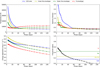 |
Fig. 16 Evolution of the temperature (upper left panel), electron fraction (upper right panel), and radioactive energy deposition (lower left panel) in the oxygen core (blue), in the inner and outer (yellow and green) helium envelope, and in the hydrogen envelope (red) for the optimal model (M17-s-s-XH-low). In the lower right panel, we show the evolution of the (Rosseland mean) continuum photosphere (black) and the outer borders of the carbon-oxygen core (blue) and the inner and outer (green and yellow) helium envelope. |
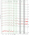 |
Fig. 17 Spectral evolution for the optimal model (M17-s-s-XH-low; black) compared to the observations of SN 2020acat (red). Spectra from ten logarithmically spaced epochs between 15 and 200 days and a single epoch at 400 days are shown. In addition, the rest wavelengths of the most important lines are shown as dashed green lines. |
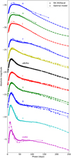 |
Fig. 18 Broad-band and bolometric light curves until 250 days for the optimal model (M17-s-s-XH-low; solid lines and circles) compared to the observations of SN 2020acat (dashed lines and crosses). From bottom to top, we show the UVM2 (magenta), u (cyan), B (blue), V (green), r (red), ugBVriz pseudo-bolometric (black), i (yellow), z (blue), J (red), H (green), and K (blue) light curves. They are shifted for clarity by 6.0, 4.3, 2.0, 0.0, −2.3, −5.7, −7.7, −10.0, −13.0, −15.0, and −17.0 mags, respectively. |
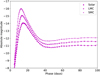 |
Fig. 19 UVM2 light curves for JEKYLL models with solar (circles), LMC (crosses), and SMC (pluses) metallicity. |
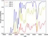 |
Fig. 20 Escape probability for photons emitted from the centre of the SN as a function of wavelength at 100 (red), 200 (yellow), and 400 (blue) days for the optimal model. We binned the resolution (λ/Δλ) to 62 for clarity. |
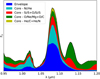 |
Fig. 21 Contributions (last emission or scattering event, excluding electron scattering) to the emission in the 1.1 μm feature from the envelope (blue) and the Ni/He (cyan), Si/S+O/Si/S (red), O/Ne/Mg+O/C (green), and He/C+He/N (yellow) zones in the core for the optimal model of SN 2020acat at 150 days. |
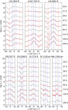 |
Fig. 22 Evolution of calcium, oxygen, and magnesium lines for the optimal model (M17-s-s-XH-low; black) compared to the observations of SN 2020acat (red). Spectra from nine logarithmically spaced epochs between 20 and 200 days are shown. The figure is otherwise the same as Fig. 13. |
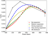 |
Fig. 23 Evolution of the luminosity in the [O I] 6300, 6364 Å lines normalised with the 56Ni decay luminosity for the JEKYLL models that differ in the expansion of the radioactive material compared to the observations of SN 2020acat (black crosses). We also show a model with very strong (a contrast factor of 210) expansion of the radioactive material in the core. |
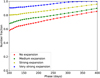 |
Fig. 24 Evolution of the fraction of O I in the oxygen-rich clumps for the JEKYLL models that differ in the expansion of the radioactive material. We also show a model with very strong (a contrast factor of 210) expansion of the radioactive material in the core. |
5 Conclusions
We presented a set of type IIb SN models calculated with the NLTE light-curve and spectral synthesis code JEKYLL and compare them to observations of the type IIb SN 2020acat. The bulk of the observations were adopted from M22 and M23, but we also presented new late-time optical observations and refined the photometry by applying S-corrections. To constrain the SN parameters for SN 2020acat, we explored a parameter space in initial mass, mixing, and expansion of the radioactive material and the mass of the hydrogen envelope and the mass-fraction of hydrogen therein. In our phenomenological models, which are based on results from hydrodynamical models, the kinetic energy is fixed by the observed velocities.
The comparisons show that a model with an initial mass of 17 M⊙, strong mixing and expansion of the radioactive material, and an 0.1 M⊙ hydrogen envelope with a low hydrogen mass-fraction (XH = 0.027) agrees best overall with the observations of SN 2020acat. Models with initial masses below 15 M⊙ and above 19 M⊙ seem to be excluded, as are models without strong expansion and at least medium mixing of the radioactive material. To be more precise, in our model grid, the strong-expansion scenario corresponds to a contrast factor of 60 in the core and 30 in the envelope, and the medium-mixing scenario corresponds to 50% of the radioactive material mixed into the inner half of the helium envelope. We note, however, that the required degree of expansion depends on the assumed clump size, and larger clumps would require weaker expansion.
Nevertheless, the strong expansion of the clumps containing radioactive material is a particularly interesting result. Without strong expansion of the Ni bubbles, there is a tension between the diffusion phase and the subsequent evolution, and models that fit the nebular phase give rise to diffusion peaks that are too broad. This is in line with the results for SN 2011dh in E22, where models without strong expansion resulted in broader diffusion peaks than observed. As discussed in detail in E22, the expansion of the Ni bubbles decreases the effective opacity and the diffusion time, and the width of the diffusion peak is therefore sensitive to this. The effect of the expansion of the Ni bubbles on the diffusion phase light curves has not been taken into account in previous light-curve modelling of type IIb and other SE SNe, and their ejecta masses might therefore have been systematically underestimated. We caution that the magnitude of the effect is uncertain, depends on weakly constrained properties of the 3D ejecta structure, and might vary in different SNe, however, so that further work is needed.
A tension between the diffusion phase and the tail phase as we found for SN 2020acat has been reported for other SE SNe (e.g. Wheeler et al. 2015; Nagy 2022), and in particular, for type Ic-BL SNe (e.g. Maeda et al. 2003; Dessart et al. 2017). Typically, large-scale asymmetries have been proposed to explain this. Because JEKYLL currently assumes a geometry that is spherically symmetric on average, we cannot rule out that large-scale asymmetries play a role in the case of SN 2020acat, and some evidence may also point in this direction. However, we showed that small-scale asymmetries caused by expansion of the radioactive material may naturally resolve the tension and provide an alternative explanation. To fully understand the role played by small- and large-scale asymmetries in the ejecta and to disentangle their effects on the observed light curves and spectra of SE SNe, full-fledged 3D NLTE simulations, preferably based on 3D explosion models, are needed.
A detailed comparison of our optimal model with the observations of SN 2020acat was presented. The overall agreement is reasonably good, although distinct differences also exist. For example, our models do not fully reproduce the evolution of the flux in the [O I] 6300, 6364 Å lines, which is faster in SN 2020acat. A quite strong discrepancy between the optimal model and the observations of SN 2020acat also emerges in the Band V-band light curves towards ~200 days, although the agreement improves again towards ~400 days. In addition, a growing excess emerges in the K band after ~100 days. This excess is reminiscent of SN 2011dh, where an IR excess attributed to dust developed at a similar timescale (see Ergon et al. 2015; Jerkstrand et al. 2015). Finally, our models are unable to reproduce the flat-topped line-profile of He I 1.083 μm that emerges after ~100 days, as discussed in M23. This might be interpreted as evidence of extreme mixing of the explosive nuclear burning material out of the carbon-oxygen core, but explosive nuclear burning in conditions different from those in the Woosley & Heger (2007) models could also help to reduce helium emission from the core.
The relatively high initial mass of ~17 M⊙ estimated for the progenitor of SN 2020acat places it at the upper end of the mass distribution of type IIb SN progenitors. Jerkstrand et al. (2015) estimated initial masses well below 17 M0 for the progenitors of SNe 2008ax, 2011dh, and 1993J using modelling of their nebular spectra, which for the latter two is supported by stellar evolutionary analysis of pre-explosion imaging of the progenitors. At the relatively high initial mass estimated for the progenitor of SN 2020acat, a single-star origin cannot be excluded. The low estimated mass fraction of hydrogen in the hydrogen envelope may be more in line with a binary origin, however. The modelling presented in this paper further demonstrates the capabilities of the JEKYLL code of self-consistently modelling the evolution of SNe from early to late times, and how this can be used to constrain the properties of SNe and their progenitor stars.
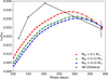 |
Fig. 25 Evolution of the luminosity in the [O I] 6300, 6364 Å lines normalised with the 56Ni decay luminosity for JEKYLL models with 56Ni masses of 0.1, 0.13, and 0.15 M⊙ compared to the observations of SN 2020acat (black crosses). |
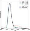 |
Fig. 26 – [O I] 6300, 6364 Å and [N II] 6548, 6583 lines at 400 days normalised to the peak flux of the former for the JEKYLL models that differ in initial mass compared to the observations of SN 2020acat. |
Acknowledgements
This work has been supported by grants from the Swedish Research Council and the Swedish National Space Board, and the computations were performed with resources provided by the Swedish National Infrastructure for Computing (SNIC) at Parallelldator-centrum (PDC). H.K was funded by the Academy of Finland projects 324504 and 328898. K.M. acknowledges support from the Japan Society for the Promotion of Science (JSPS) KAKENHI grant JP18H05223, JP20H00174, and JP20H04737. K.M. and H.K. acknowledge support by the JSPS Open Partnership Bilateral Joint Research Projects between Japan and Finland (JPJSBP120229923). A.P. acknowledges support from PRIN-INAF 2022 project "Exploring new frontiers of the transient universe in the era of synoptic surveys". M.S. is funded by the Independent Research Fund Denmark (IRFD), grant number 10.46540/2032-00022B). We also thank Luc Dessart for fruitful and always interesting discussions on the effect of clumping on the light curves and spectra of SNe, and Anders Jerkstrand for providing the base for the 13 and 17 M⊙ models as well as parts of the atomic data used in the simulations.
Appendix A Configuration
JEKYLL was configured to run in time-dependent mode (with respect to the radiative transfer), and to use a full NLTE solution including radiative bound-bound, bound-free, and free-free processes, collisional bound-bound and bound-free processes, non-thermal excitation, ionisation, and heating, as well as two-photon processes and charge transfer. Before 100 days, charge-transfer was not included, however, and non-thermal excitation was only included for He. The diffusion solver was used above an optical depth of 50, and a recombination correction based on the total recombination rates was used while still enforcing detailed balance. In addition, packet control (E18,) was turned on to ensure good sampling of the radiation field in all frequency regions. The number of Λ-iterations per time step was set to 4. As discussed in E18, this gives a well-converged solution that was also verified for the models used in this paper.
Appendix B Atomic data
The atomic dataset we used is the default choice described in E18, but was extended with more levels and a full NLTE solution for ionisation stages V and VI. This makes only a small difference for the observed light curves and spectra, and tests show that the simulations are not sensitive to further changes in the number of levels and ionisation stages. Using online data provided by NIST4 (National Institute of Standards and Technology) and R. Kurucz5, these ions were updated to include 100 levels (or as many as were available) for elements lighter than scandium and 300 levels (or as many as were available) for heavier elements. The total recombination rates for these ions were adopted from the online table provided by S. Nahar6 whenever available, and from Shull & van Steenberg (1982) otherwise.
Appendix C Ejecta models
In Table C.1 we list the mass and in Tables C.2–C.6 the composition for each zone in our models with initial masses of 13, 15, 17, 19, and 21 M⊙. The ejecta mass and (kinetic) energy of these models are also listed in Table C.1. We note that expect for the interface velocities and the mass of the Ni/He zone, the 13 and 17 M⊙ models are adopted from Jerkstrand et al. (2015).
Ejecta mass (M⊙), (kinetic) ejecta energy (B), and zone masses (M⊙) for models with initial masses of 13, 15, 17, 19, and 21 M⊙.
Zone composition for models with an initial mass of 13 M⊙.
Zone composition for models with an initial mass of 15 M⊙.
Zone composition for models with an initial mass of 17 M⊙.
Zone composition for models with an initial mass of 19 M⊙.
Zone composition for models with an initial mass of 21 M⊙.
Appendix D Additional spectral figures
For convenience, we provide a set of additional spectral figures for the optimal model of SN 2020acat. First, we show in Fig. D.1 the contribution (last scattering or emission event, excluding electron scattering) from the carbon-oxygen core, the inner and outer helium envelope, and the hydrogen envelope to the spectral evolution.
Second, we show in Fig. D.2–D.7 the bound-bound contribution (last scattering or emission event, excluding electron scattering) from ionisation stages I, II, III, and higher of hydrogen, helium, carbon, nitrogen, oxygen, sodium, magnesium, silicon, sulphur, calcium, scandium, titanium, chromium, manganese, iron, cobalt, nickel, and other elements to the spectral evolution.
Finally, in Fig. D.8 we show the bound-bound contribution (last scattering or emission event excluding electron scattering) from the nickel-rich (Ni/He, Si/S), oxygen-rich (O/Si/S, O/Ne/Mg, O/C), and hydrogen- and helium-rich (He/C, He/N, H) compositional zones to the spectral evolution.
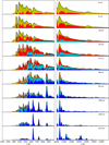 |
Fig. D.1 Spectral evolution in the optical (left panel) and NIR (right panel) for the optimal model, where the NIR flux has been scaled as indicated in blue. In the spectra, we show the contributions (last scattering or emission event, excluding electron scattering) to the flux from the carbon-oxygen core (blue), the inner (cyan) and outer (red) helium envelope, and the hydrogen (yellow) envelopes. |
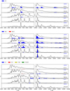 |
Fig. D.2 Bound-bound contribution from ionisation stages I (blue), II (red), III (yellow), and higher (green) of hydrogen (upper panel), helium (middle panel), and carbon (lower panel) to the spectral evolution of the optimal model. |
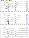 |
Fig. D.3 Bound-bound contribution from ionisation stages I (blue), II (red), III (yellow), and higher (green) of nitrogen (upper panel), oxygen (middle panel), and sodium (lower panel) to the spectral evolution of the optimal model. |
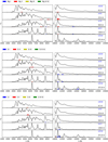 |
Fig. D.4 Bound-bound contribution from ionisation stages I (blue), II (red), III (yellow), and higher (green) of magnesium (upper panel), silicon (middle panel), and sulphur (lower panel) to the spectral evolution of the optimal model. |
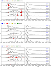 |
Fig. D.5 Bound-bound contribution from ionisation stages I (blue), II (red), III (yellow), and higher (green) of calcium (upper panel), scandium (middle panel), and titanium (lower panel) to the spectral evolution of the optimal model. |
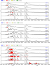 |
Fig. D.6 Bound-bound contribution from ionisation stages I (blue), II (red), III (yellow), and higher (green) of chromium (upper panel), manganese (middle panel), and iron (lower panel) to the spectral evolution of the optimal model. |
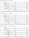 |
Fig. D.7 Bound-bound contribution from ionisation stages I (blue), II (red), III (yellow), and higher (green) of cobalt (upper panel), nickel (middle panel), and other elements (lower panel) to the spectral evolution of the optimal model. |
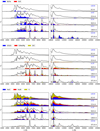 |
Fig. D.8 Bound-bound contribution from the nickel-rich zones (Ni/He: blue, Si/S: red), the oxygen-rich zones (O/Si/S: blue, O/Ne/Mg: red, O/C: yellow), and the hydrogen- and helium-rich zones (H/C: blue, He/N: red, H: yellow) to the spectral evolution of the optimal model. |
References
- Aldering, G., Humphreys, R. M., & Richmond, M. 1994, AJ, 107, 662 [Google Scholar]
- Arcavi, I., Gal-Yam, A., Yaron, O., et al. 2011, ApJ, 742, L18 [Google Scholar]
- Arnett, W. D. 1982, ApJ, 253, 785 [Google Scholar]
- Bersten, M. C., Benvenuto, O., & Hamuy, M. 2011, ApJ, 729, 61 [NASA ADS] [CrossRef] [Google Scholar]
- Bersten, M. C., Benvenuto, O. G., Nomoto, K., et al. 2012, ApJ, 757, 31 [Google Scholar]
- Brown, T. M., Baliber, N., Bianco, F. B., et al. 2013, PASP, 125, 1031 [Google Scholar]
- Cano, Z. 2013, MNRAS, 434, 1098 [Google Scholar]
- Chugai, N. N. 1994, ApJ, 428, L17 [NASA ADS] [CrossRef] [Google Scholar]
- De, K., Kasliwal, M. M., Tzanidakis, A., et al. 2020, ApJ, 905, 58 [NASA ADS] [CrossRef] [Google Scholar]
- Dessart, L., & Audit, E. 2019, A&A, 629, A17 [NASA ADS] [CrossRef] [EDP Sciences] [Google Scholar]
- Dessart, L., Hillier, D. J., Yoon, S.-C., Waldman, R., & Livne, E. 2017, A&A, 603, A51 [NASA ADS] [CrossRef] [EDP Sciences] [Google Scholar]
- Dessart, L., Hillier, D. J., & Wilk, K. D. 2018, A&A, 619, A30 [NASA ADS] [CrossRef] [EDP Sciences] [Google Scholar]
- Ennis, J. A., Rudnick, L., Reach, W. T., et al. 2006, ApJ, 652, 376 [NASA ADS] [CrossRef] [Google Scholar]
- Ergon, M. 2015, PhD thesis, Stockholm University, Sweden [Google Scholar]
- Ergon, M., & Fransson, C. 2022, A&A, 666, A104 [NASA ADS] [CrossRef] [EDP Sciences] [Google Scholar]
- Ergon, M., Sollerman, J., Fraser, M., et al. 2014, A&A, 562, A17 [NASA ADS] [CrossRef] [EDP Sciences] [Google Scholar]
- Ergon, M., Jerkstrand, A., Sollerman, J., et al. 2015, A&A, 580, A142 [NASA ADS] [CrossRef] [EDP Sciences] [Google Scholar]
- Ergon, M., Fransson, C., Jerkstrand, A., et al. 2018, A&A, 620, A156 [NASA ADS] [CrossRef] [EDP Sciences] [Google Scholar]
- Fransson, C., & Chevalier, R. A. 1989, ApJ, 343, 323 [NASA ADS] [CrossRef] [Google Scholar]
- Freudling, W., Romaniello, M., Bramich, D. M., et al. 2013, A&A, 559, A96 [NASA ADS] [CrossRef] [EDP Sciences] [Google Scholar]
- Fryxell, B., Mueller, E., & Arnett, D. 1991, ApJ, 367, 619 [NASA ADS] [CrossRef] [Google Scholar]
- Höflich, P., Wheeler, J. C., & Wang, L. 1999, ApJ, 521, 179 [CrossRef] [Google Scholar]
- Jerkstrand, A., Fransson, C., & Kozma, C. 2011, A&A, 530, A45 [NASA ADS] [CrossRef] [EDP Sciences] [Google Scholar]
- Jerkstrand, A., Fransson, C., Maguire, K., et al. 2012, A&A, 546, A28 [NASA ADS] [CrossRef] [EDP Sciences] [Google Scholar]
- Jerkstrand, A., Ergon, M., Smartt, S. J., et al. 2015, A&A, 573, A12 [NASA ADS] [CrossRef] [EDP Sciences] [Google Scholar]
- Kozma, C., & Fransson, C. 1992, ApJ, 390, 602 [NASA ADS] [CrossRef] [Google Scholar]
- Kozma, C., & Fransson, C. 1998, ApJ, 497, 431 [NASA ADS] [CrossRef] [Google Scholar]
- Kromer, M., & Sim, S. A. 2009, MNRAS, 398, 1809 [Google Scholar]
- Kuncarayakti, H., Maeda, K., Dessart, L., et al. 2022, ApJ, 941, L32 [NASA ADS] [CrossRef] [Google Scholar]
- Lucy, L. B. 2002, A&A, 384, 725 [NASA ADS] [CrossRef] [EDP Sciences] [Google Scholar]
- Lucy, L. B. 2003, A&A, 403, 261 [NASA ADS] [CrossRef] [EDP Sciences] [Google Scholar]
- Lucy, L. B. 2005, A&A, 429, 19 [NASA ADS] [CrossRef] [EDP Sciences] [Google Scholar]
- Lyman, J. D., Bersier, D., James, P. A., et al. 2016, MNRAS, 457, 328 [Google Scholar]
- Maeda, K., Mazzali, P. A., Deng, J., et al. 2003, ApJ, 593, 931 [NASA ADS] [CrossRef] [Google Scholar]
- Matheson, T., Filippenko, A. V., Ho, L. C., Barth, A. J., & Leonard, D. C. 2000, AJ, 120, 1499 [NASA ADS] [CrossRef] [Google Scholar]
- Mauerhan, J. C., Williams, G. G., Leonard, D. C., et al. 2015, MNRAS, 453, 4467 [CrossRef] [Google Scholar]
- Maund, J. R., Fraser, M., Ergon, M., et al. 2011, ApJ, 739, L37 [Google Scholar]
- Medler, K., Mazzali, P. A., Teffs, J., et al. 2022, MNRAS, 513, 5540 [NASA ADS] [CrossRef] [Google Scholar]
- Medler, K., Mazzali, P. A., Ashall, C., et al. 2023, MNRAS, 518, L40 [Google Scholar]
- Milisavljevic, D., & Fesen, R. A. 2013, ApJ, 772, 134 [Google Scholar]
- Milisavljevic, D., & Fesen, R. A. 2015, Science, 347, 526 [NASA ADS] [CrossRef] [Google Scholar]
- Nagy, A. P. 2022, MNRAS, submitted. [arXiv:2218.18458] [Google Scholar]
- Perley, D. A. 2019, PASP, 131, 084503 [Google Scholar]
- Pessi, P., Anderson, J. P., Galbany, L., & Irani, I. 2020, Transient Name Server Classification Report, 2020-3741, 1 [Google Scholar]
- Prentice, S. J., Mazzali, P. A., Pian, E., et al. 2016, MNRAS, 458, 2973 [NASA ADS] [CrossRef] [Google Scholar]
- Shull, J. M., & van Steenberg, M. 1982, ApJS, 48, 95 [NASA ADS] [CrossRef] [Google Scholar]
- Spyromilio, J., & Pinto, P. A. 1991, European Southern Observatory Conference and Workshop Proceedings, 37, 423 [NASA ADS] [Google Scholar]
- Srivastav, S., Smith, K. W., McBrien, O., et al. 2020, Transient Name Server AstroNote, 249, 1 [NASA ADS] [Google Scholar]
- Stritzinger, M., Hamuy, M., Suntzeff, N. B., et al. 2002, AJ, 124, 2100 [NASA ADS] [CrossRef] [Google Scholar]
- Taddia, F., Stritzinger, M. D., Bersten, M., et al. 2018, A&A, 609, A136 [NASA ADS] [CrossRef] [EDP Sciences] [Google Scholar]
- Valenti, S., Benetti, S., Cappellaro, E., et al. 2008, MNRAS, 383, 1485 [Google Scholar]
- Wheeler, J. C., Johnson, V., & Clocchiatti, A. 2015, MNRAS, 450, 1295 [Google Scholar]
- Willingale, R., Bleeker, J. A. M., van der Heyden, K. J., Kaastra, J. S., & Vink, J. 2002, A&A, 381, 1039 [NASA ADS] [CrossRef] [EDP Sciences] [Google Scholar]
- Wongwathanarat, A., Janka, H.-T., Müller, E., Pllumbi, E., & Wanajo, S. 2017, ApJ, 842, 13 [Google Scholar]
- Woosley, S. E., & Heger, A. 2007, Phys. Rep., 442, 269 [Google Scholar]
- Woosley, S. E., Eastman, R. G., Weaver, T. A., & Pinto, P. A. 1994, ApJ, 429, 300 [NASA ADS] [CrossRef] [Google Scholar]
- Yoon, S. C., Woosley, S. E., & Langer, N. 2010, ApJ, 725, 940 [NASA ADS] [CrossRef] [Google Scholar]
Here and in the following, tension refers to a difference in results derived from fitting the early and late phase, that is, some shortcomings in the models that prevent a simultaneous fitting of these two phases.
With 'state of matter' we refer to the temperature and the populations of ionised and excited states.
Because the outer part of the hydrogen envelope was removed after 100 days (see Sect. 3.4), it was not included in the average.
All Tables
Light-curve characteristics for the pseudo-bolometric uBVriz light curves of SN 2020acat and SN 2011dh measured from cubic spline fits.
Ejecta mass (M⊙), (kinetic) ejecta energy (B), and zone masses (M⊙) for models with initial masses of 13, 15, 17, 19, and 21 M⊙.
All Figures
|
Fig. 1 Broadband and bolometric light curves until 250 days for SN 2020acat (filled circles) compared to SN 2011dh (empty squares). From bottom to top, we show the UVM2 (magenta), u (cyan), B (blue), V (green), r (red), ugBVriz pseudo-bolometric (black), i (yellow), z (blue), J (red), H (green), and K (blue) light curves. They are shifted for clarity by 6.0, 4.3, 2.0, 0.0, −2.3, −5.7, −7.7, −10.0, −13.0, −15.0, and −17.0 mags, respectively. |
| In the text | |
|
Fig. 2 Spectral evolution of SN 2020acat (red) compared to SN 2011dh (black). Spectra from ten logarithmically spaced epochs between 15 and 200 days and a single epoch at 400 days are shown. In addition, the rest wavelengths of the most important lines are shown as dashed green lines. |
| In the text | |
|
Fig. 3 Comparison of the evolution of the absorption minimum for the Hα (yellow) and He I 7065 Å (blue) lines and the HWHM of the [O I] 6300, 6364Å doublet for SN 2020acat (filled circles) and SN 2011dh (empty squares). |
| In the text | |
|
Fig. 4 Comparison of the evolution of the Hα and Hβ lines in SN 2020acat and SN 2011dh. Spectra from ten equally spaced epochs between 10 and 100 days are shown. Interpolated spectra that have no observed counterpart close in time are shown in grey. The inferred helium-hydrogen interface velocities of SNe 2011dh (11 000 km s−1) and 2020acat (12 000 km s−1) are shown as dashed red lines. |
| In the text | |
|
Fig. 5 Comparison of the evolution of the He I 5876 Å and He I 10 830 Å lines in SN 2020acat and SN 2011dh. Spectra from ten equally spaced epochs between 10 and 150 days are shown. Otherwise, this is the same as in Fig. 4. |
| In the text | |
|
Fig. 6 Comparison of the evolution of the [O I] 6300, 6364 Å luminosity normalised with the pseudo-bolometric uBVriz luminosity (upper panel) and the 56Ni decay-chain luminosity (lower panel) for SN 2020acat (filled circles) and SN 2011dh (empty squares). |
| In the text | |
|
Fig. 7 Evolution of the luminosity in the [O I] 6300, 6364 Å lines normalised with the 56Ni decay luminosity for SN 2020acat (black crosses) and the JEKYLL models with strong expansion and medium mixing of the radioactive material and initial masses of 13 M⊙ (red), 15 M⊙ (cyan), 17 M⊙ (green), 19 M⊙ (yellow), and 21 M⊙ (blue). |
| In the text | |
|
Fig. 8 Evolution of the luminosity in the [Ca II] 7291, 7323 Å lines normalised with 56Ni decay luminosity for SN 2020acat (black crosses) and the JEKYLL models with strong expansion and medium mixing of the radioactive material and initial masses of 13 M⊙ (red), 15 M⊙ (cyan), 17 M⊙ (green), 19 M⊙ (yellow), and 21 M⊙ (blue). |
| In the text | |
|
Fig. 9 Pseudo-bolometric uBVriz light curves until 250 days for SN 2020acat and JEKYLL models with strong expansion and medium mixing of the radioactive material and initial masses of 13 M⊙ (red), 15 M⊙ (cyan), 17 M⊙ (green), 19 M⊙ (yellow), and 21 M⊙ (blue). |
| In the text | |
|
Fig. 10 Pseudo-bolometric uBVriz light curves until 150 days for SN 2020acat and JEKYLL models with an initial mass of 17 M⊙, medium mixing, and no, medium, and strong expansion of the radioactive material. |
| In the text | |
|
Fig. 11 Pseudo-bolometric uBVriz light curves until 150 days for SN 2020acat and JEKYLL models with an initial mass of 17 M⊙, no expansion, and weak, medium, and strong mixing of the radioactive material. |
| In the text | |
|
Fig. 12 Pseudo-bolometric uBVriz light curves until 150 days for SN 2020acat and JEKYLL models with an initial mass of 17 M⊙, strong expansion, and weak, medium, and strong mixing of the radioactive material. |
| In the text | |
|
Fig. 13 Evolution of the Hα (upper panel) and Hβ (lower panel) lines for SN 2020acat (red) and the JEKYLL models (black) with an initial mass of 17 M⊙, strong mixing and strong expansion of the radioactive material, and a mass of hydrogen in the envelope of 0.0135 (left), 0.027 (middle), and 0.054 (right) M⊙. Spectra from nine logarithmically spaced epochs are shown, and the model C/O-He (blue) and He-H (red) interface velocities are indicated with dashed lines. |
| In the text | |
|
Fig. 14 Evolution of the He I 5876 Å (upper panel) and He I 1.083 μm (lower panel) lines for SN 2020acat (red) and the JEKYLL models (black) with an initial mass of 17 M⊙, strong expansion of the radioactive material, medium mixing plus XH =0.54 (left), strong mixing plus XH = 0.54 (middle), and strong mixing plus XH = 0.27 (right). The figure is otherwise the same as Fig. 13. |
| In the text | |
|
Fig. 15 Evolution of the (mass-averaged) effective Rosseland mean opacity in the inner helium envelope for the model with strong expansion (black) and the corresponding effective Rosseland mean opacity in the limits of optically thick (blue) and thin (red) clumps. In addition, we show the evolution of the effective Rosseland mean opacity for the model without expansion (cyan). |
| In the text | |
|
Fig. 16 Evolution of the temperature (upper left panel), electron fraction (upper right panel), and radioactive energy deposition (lower left panel) in the oxygen core (blue), in the inner and outer (yellow and green) helium envelope, and in the hydrogen envelope (red) for the optimal model (M17-s-s-XH-low). In the lower right panel, we show the evolution of the (Rosseland mean) continuum photosphere (black) and the outer borders of the carbon-oxygen core (blue) and the inner and outer (green and yellow) helium envelope. |
| In the text | |
|
Fig. 17 Spectral evolution for the optimal model (M17-s-s-XH-low; black) compared to the observations of SN 2020acat (red). Spectra from ten logarithmically spaced epochs between 15 and 200 days and a single epoch at 400 days are shown. In addition, the rest wavelengths of the most important lines are shown as dashed green lines. |
| In the text | |
|
Fig. 18 Broad-band and bolometric light curves until 250 days for the optimal model (M17-s-s-XH-low; solid lines and circles) compared to the observations of SN 2020acat (dashed lines and crosses). From bottom to top, we show the UVM2 (magenta), u (cyan), B (blue), V (green), r (red), ugBVriz pseudo-bolometric (black), i (yellow), z (blue), J (red), H (green), and K (blue) light curves. They are shifted for clarity by 6.0, 4.3, 2.0, 0.0, −2.3, −5.7, −7.7, −10.0, −13.0, −15.0, and −17.0 mags, respectively. |
| In the text | |
|
Fig. 19 UVM2 light curves for JEKYLL models with solar (circles), LMC (crosses), and SMC (pluses) metallicity. |
| In the text | |
|
Fig. 20 Escape probability for photons emitted from the centre of the SN as a function of wavelength at 100 (red), 200 (yellow), and 400 (blue) days for the optimal model. We binned the resolution (λ/Δλ) to 62 for clarity. |
| In the text | |
|
Fig. 21 Contributions (last emission or scattering event, excluding electron scattering) to the emission in the 1.1 μm feature from the envelope (blue) and the Ni/He (cyan), Si/S+O/Si/S (red), O/Ne/Mg+O/C (green), and He/C+He/N (yellow) zones in the core for the optimal model of SN 2020acat at 150 days. |
| In the text | |
|
Fig. 22 Evolution of calcium, oxygen, and magnesium lines for the optimal model (M17-s-s-XH-low; black) compared to the observations of SN 2020acat (red). Spectra from nine logarithmically spaced epochs between 20 and 200 days are shown. The figure is otherwise the same as Fig. 13. |
| In the text | |
|
Fig. 23 Evolution of the luminosity in the [O I] 6300, 6364 Å lines normalised with the 56Ni decay luminosity for the JEKYLL models that differ in the expansion of the radioactive material compared to the observations of SN 2020acat (black crosses). We also show a model with very strong (a contrast factor of 210) expansion of the radioactive material in the core. |
| In the text | |
|
Fig. 24 Evolution of the fraction of O I in the oxygen-rich clumps for the JEKYLL models that differ in the expansion of the radioactive material. We also show a model with very strong (a contrast factor of 210) expansion of the radioactive material in the core. |
| In the text | |
|
Fig. 25 Evolution of the luminosity in the [O I] 6300, 6364 Å lines normalised with the 56Ni decay luminosity for JEKYLL models with 56Ni masses of 0.1, 0.13, and 0.15 M⊙ compared to the observations of SN 2020acat (black crosses). |
| In the text | |
|
Fig. 26 – [O I] 6300, 6364 Å and [N II] 6548, 6583 lines at 400 days normalised to the peak flux of the former for the JEKYLL models that differ in initial mass compared to the observations of SN 2020acat. |
| In the text | |
|
Fig. D.1 Spectral evolution in the optical (left panel) and NIR (right panel) for the optimal model, where the NIR flux has been scaled as indicated in blue. In the spectra, we show the contributions (last scattering or emission event, excluding electron scattering) to the flux from the carbon-oxygen core (blue), the inner (cyan) and outer (red) helium envelope, and the hydrogen (yellow) envelopes. |
| In the text | |
|
Fig. D.2 Bound-bound contribution from ionisation stages I (blue), II (red), III (yellow), and higher (green) of hydrogen (upper panel), helium (middle panel), and carbon (lower panel) to the spectral evolution of the optimal model. |
| In the text | |
|
Fig. D.3 Bound-bound contribution from ionisation stages I (blue), II (red), III (yellow), and higher (green) of nitrogen (upper panel), oxygen (middle panel), and sodium (lower panel) to the spectral evolution of the optimal model. |
| In the text | |
|
Fig. D.4 Bound-bound contribution from ionisation stages I (blue), II (red), III (yellow), and higher (green) of magnesium (upper panel), silicon (middle panel), and sulphur (lower panel) to the spectral evolution of the optimal model. |
| In the text | |
|
Fig. D.5 Bound-bound contribution from ionisation stages I (blue), II (red), III (yellow), and higher (green) of calcium (upper panel), scandium (middle panel), and titanium (lower panel) to the spectral evolution of the optimal model. |
| In the text | |
|
Fig. D.6 Bound-bound contribution from ionisation stages I (blue), II (red), III (yellow), and higher (green) of chromium (upper panel), manganese (middle panel), and iron (lower panel) to the spectral evolution of the optimal model. |
| In the text | |
|
Fig. D.7 Bound-bound contribution from ionisation stages I (blue), II (red), III (yellow), and higher (green) of cobalt (upper panel), nickel (middle panel), and other elements (lower panel) to the spectral evolution of the optimal model. |
| In the text | |
|
Fig. D.8 Bound-bound contribution from the nickel-rich zones (Ni/He: blue, Si/S: red), the oxygen-rich zones (O/Si/S: blue, O/Ne/Mg: red, O/C: yellow), and the hydrogen- and helium-rich zones (H/C: blue, He/N: red, H: yellow) to the spectral evolution of the optimal model. |
| In the text | |
Current usage metrics show cumulative count of Article Views (full-text article views including HTML views, PDF and ePub downloads, according to the available data) and Abstracts Views on Vision4Press platform.
Data correspond to usage on the plateform after 2015. The current usage metrics is available 48-96 hours after online publication and is updated daily on week days.
Initial download of the metrics may take a while.