| Issue |
A&A
Volume 675, July 2023
|
|
|---|---|---|
| Article Number | A206 | |
| Number of page(s) | 18 | |
| Section | Interstellar and circumstellar matter | |
| DOI | https://doi.org/10.1051/0004-6361/202346241 | |
| Published online | 24 July 2023 | |
A panoptic view of the Taurus molecular cloud
I. The cloud dynamics revealed by gas emission and 3D dust
1
Istituto di Astrofisica e Planetologia Spaziali (IAPS), INAF,
Via Fosso del Cavaliere 100,
00133
Roma, Italy
e-mail: soler@mpia.de
2
Space Telescope Science Institute,
3700 San Martin Drive,
Baltimore, MD
21218, USA
3
Astronomy Department, University of Massachusetts,
Amherst, MA
01003, USA
4
Jet Propulsion Laboratory, California Institute of Technology,
4800 Oak Grove Drive,
Pasadena, CA
91109, USA
5
Universität Heidelberg, Zentrum für Astronomie, Institut für Theoretische Astrophysik,
Albert-Ueberle-Str. 2,
69120
Heidelberg, Germany
6
Universität Heidelberg, Interdiszipliäres Zentrum für Wissenschaftliches Rechnen,
Im Neuenheimer Feld 205,
69120
Heidelberg, Germany
7
Laboratoire AIM, Paris-Saclay, CEA/IRFU/SAp - CNRS - Université Paris-Diderot,
91191
Gif-sur-Yvette Cedex, France
8
Dipartimento di Fisica e Astronomia, Università di Bologna,
Via Gobetti 93/2,
40122
Bologna, Italy
Received:
24
February
2023
Accepted:
22
May
2023
We present a study of the three-dimensional (3D) distribution of interstellar dust derived from stellar extinction observations toward the Taurus molecular cloud (MC) and its relation with the neutral atomic hydrogen (H I) emission at 21 cm wavelength and the carbon monoxide 12CO and 13CO emission in the J = 1 → 0 transition. We used the histogram of oriented gradients (HOG) method to match the morphology in a 3D reconstruction of the dust density (3D dust) and the distribution of the gas tracers’ emission. The result of the HOG analysis is a map of the relationship between the distances and radial velocities. The HOG comparison between the 3D dust and the H I emission indicates a morphological match at the distance of Taurus but an anticorrelation between the dust density and the H I emission, which uncovers a significant amount of cold H I within the Taurus MC. The HOG study between the 3D dust and 12CO reveals a pattern in radial velocities and distances that is consistent with converging motions of the gas in the Taurus MC, with the near side of the cloud moving at higher velocities and the far side moving at lower velocities. This convergence of flows is likely triggered by the large-scale gas compression caused by the interaction of the Local Bubble and the Per-Tau shell, with Taurus lying at the intersection of the two bubble surfaces.
Key words: ISM: clouds / ISM: structure / ISM: molecules / ISM: kinematics and dynamics / stars: formation / dust, extinction
© The Authors 2023
 Open Access article, published by EDP Sciences, under the terms of the Creative Commons Attribution License (https://creativecommons.org/licenses/by/4.0), which permits unrestricted use, distribution, and reproduction in any medium, provided the original work is properly cited.
This article is published in open access under the Subscribe to Open model. Subscribe to A&A to support open access publication.
1 Introduction
Most stars form in a cold, dense, and mostly molecular phase of the interstellar medium (ISM; see, Ferrière 2001; Klessen & Glover 2016, for a review). Although there is a significant amount of diffuse molecular gas in the Milky Way and other galaxies (see, for example, Roman-Duval et al. 2016; Miville-Deschênes et al. 2017; Rosolowsky et al. 2021), most of the star formation appears related to localized dense molecular clouds (MCs; see, Dobbs et al. 2014; Heyer & Dame 2015; Chevance et al. 2022, for a review). Thus, insight into the formation and destruction of MCs is crucial for understanding the star formation process and the evolution of galaxies. For this paper, we combined the atomic and molecular gas emission with the dust three-dimensional (3D) distribution in and around the Taurus MC in search of clues about its formation and current dynamics.
At a distance of around 140 pc (Zucker et al. 2020), Taurus is one of the nearest and best-studied star-forming regions (see Kenyon et al. 2008, for a review). It was first discovered as a series of dark spots and lanes visible against the bright background of stars just south of the Milky Way’s plane (Barnard 1919; Lynds 1962) and is one of the MCs where the relation between dust and gas was first studied (Lilley 1955). This region does not contain luminous O or B stars but has a rich population of less-massive pre-main sequence stars, among them T Tauri variable stars with G, K, or M spectral types (Joy 1945; Kenyon & Hartmann 1995; Rebull et al. 2010).
The first large-scale and high angular resolution study resolution of Taurus in carbon monoxide (CO) emission in the J = 1 → 0 transition revealed a mass of 2.4 × 10⁴ M⊙ in molecular gas, which in combination with the counts of young stars results in a star formation efficiency between 0.3% and 1.2% (Goldsmith et al. 2008). Observations of neutral atomic hydrogen (H I) emission toward dark clouds in Taurus reveal the presence of H I narrow self-absorption (HINSA) features that appear correlated with the hydroxyl radical (OH) and CO emission, which suggests that a significant fraction of the H I is located in the cold, well-shielded portions of MCs and is mixed with the molecular gas (Li & Goldsmith 2003; Goldsmith & Li 2005).
Three-dimensional maps of the local dust distribution in 3D indicate that the Taurus MC sits in the nearest hemisphere of a near-spherical shell with a diameter of around 160 pc that is also connected to the Perseus MC, thus called the Per-Tau shell (Leike et al. 2020; Bialy et al. 2021). The connection between the Taurus and Perseus MCs had been suggested since the first large-scale mapping of the CO emission toward these regions (Ungerechts & Thaddeus 1987). Still, it was only confirmed with the advent of the stellar parallax measurements from ESA’s Gaia satellite, which along with other observations, enable the mapping of dust in 3D (see, for example, Lallement et al. 2018; Green et al. 2019). The Per-Tau shell is most likely the result of stellar and supernova (SN) feedback that swept up the surrounding interstellar medium (ISM), leading to the accumulation of matter that formed the Perseus and Taurus MCs. Using the observations of the soft X-ray continuum and the 26Al line emission, Bialy et al. (2021) estimate that the Per-Tau shell’s age is between 6 and 22 Myr.
Recent studies presented in Zucker et al. (2022) reveal that, in addition to touching the near side of the Per-Tau shell, Taurus lies at the edge of the Local Bubble. The Local Bubble is the cavity of the low-density, high-temperature plasma surrounded by a shell of cold, neutral gas and dust in which the Sun lies (see, for example, Sanders et al. 1977; Cox & Reynolds 1987; Snowden et al. 2015; Pelgrims et al. 2020). Its expansion was most likely powered by 15 to 20 SNe that have exploded over the past 14 Myr (Zucker et al. 2022). Thus, Taurus’s position, nestled at the intersection of two shells, suggests that it may have formed by the material gathered in the collision of these two bubbles.
In this paper, we focus on the current dynamics of the Taurus MC using new data and a new method. We used the new 3D dust maps obtained with a hierarchical Bayesian model based on stellar parallax and extinction observations from Gaia and other observatories (Leike & Enßlin 2019; Leike et al. 2020). We employed the new histogram of oriented gradients (HOG; Soler et al. 2019) method to identify the correlation in the extended emission from the different tracers. We applied the HOG method to connect the distribution of the 3D dust map and the H I and CO emission toward the Taurus MC. The result is a map of the relationship between distances and radial velocities that we used to elucidate the MC dynamics. Radio emission from the ISM and 3D dust have previously been combined to investigate the ISM in four dimensions (three spatial and one velocity; Tchernyshyov & Peek 2017), but never at the level of distance precision we use here, and never before with the HOG.
This manuscript is organized as follows. We present the H I, CO, and 3D dust observations in Sect. 2. In Sect. 3, we summarize the main aspects of the astroHOG method and introduce the circular statistical tools used to quantify the correlation between the observations. Section 4 presents the results of the comparison between the gas tracers and the 3D dust model. We present a discussion of our results and their implication for the understanding of the Taurus region and other MCs in Sect. 5. Finally, we present our conclusions in Sect. 6. We reserve complementary analysis to a set of appendices. Appendix A presents the tests performed to evaluate the significance of the HOG results. Appendix B shows the results of different smoothing procedures and masking procedures in the computation of the HOG. In Appendix C, we present the HOG results obtained when applying column density masks to study the morphological correlation within the extinction-based boundaries assigned to the Taurus MC. We present the HOG results obtained when dividing the region into blocks in Appendix D. Finally, Appendix E presents the results of the HOG correlation between the gas tracers and the 3D extinction maps presented in Green et al. (2019).
2 Data
2.1 Carbon monoxide (CO) emission
We used the 100 deg2 survey of the Taurus MC region in 12CO and 13CO emission in the J = 1 → 0 transition presented in Goldsmith et al. (2008). These data were obtained using the 32-pixel SEQUOIA focal plane array receiver installed in the 13.7-m Quabbin millimeter-wave telescope of the Five College Radio Astronomy Observatory (Erickson et al. 1999). The full width at half maximum (FWHM) beam sizes of the telescope are 45″ and 47″ for the frequencies of 115.271202 and 110.201353 GHz, which correspond to the emission lines 12CO(1 → 0) and 13CO(1 → 0), respectively. Further details of the data taking, data reduction, and calibration procedures are presented in Narayanan et al. (2008).
The final emission cubes of both isotopologues are very close to the Nyquist sampled and are presented in a uniform grid of 20″ spacing, with 2069 pixels in right ascension (RA) and 1529 pixels in declination (DEC). In the spectral axis, the data covers the radial velocity range between −5 and 14.9 km s−1 in 80 spectral channels for 12CO and 76 channels for 13CO, which correspond to channel widths of 0.26 and 0.27 km s−1. For these channel widths, the mean root-mean-square antenna temperatures in this data set are 0.28 K and 0.125 K for 12CO and 13CO, respectively.
2.2 Atomic hydrogen (H I) emission
We used the publicly available observations from the Galactic Arecibo L-Band Feed Array H I survey (GALFA-H I) data release 2 (DR2; Peek et al. 2018). This survey covers the H I emission from −650 to 650 km s−1, with 0.184 km s−1 channel spacing, 4′ angular resolution, and 150 mK root mean square (rms) noise per 1 km s−1 velocity channel. The GALFA-H I DR2 observations cover the entirety of the sky available from the William E. Gordon 305 m antenna at Arecibo, from δ = −1°17′ to +37°57′ across the whole right ascension (α) range. This data set provides the highest-resolution map of extended H I emission toward Taurus available to date.
We obtained the GALFA-H I DR2 distributed in FITS-format cubes in the “narrow” velocity range (υ ≤ 188 km s−1). through the GALFA collaboration website1. We used the Python spectral-cube and reproject2 packages to arrange these cubes into a 20″ grid matching the coverage of the 12CO and13 CO data, but maintaining the native spectral axis with a spectral resolution of 0.184 km s−1. This operation implies over-sampling the 4′ beam, but we accounted for this fact using the statistical weights introduced in Sect. 3.
2.3 Dust
2.3.1 3D dust
We used the 3D dust distribution cube presented in Leike et al. (2020). This model has a higher spatial resolution than other state-of-the-art 3D dust reconstructions (for example, Rezaei Kh. & Kainulainen 2022; Vergely et al. 2022; Dharmawardena et al. 2023). Since the statistical significance of the HOG analysis depends on the number of independent gradients in the compared images, this advantage is crucial for the study presented in this paper.
The Leike et al. (2020) dust cube was derived from stellar distances and integrated extinction estimates from the Starhorse catalog (Anders et al. 2019), which combined observations from ESA’s Gaia satellite second data release (DR2; Gaia Collaboration 2018), NASA’s Wide-field Infrared Survey Explorer (WISE) mission (Wright et al. 2010), the Two Micron All Sky Survey (2MASS; Skrutskie et al. 2006), and the Panoramic Survey Telescope and Rapid Response System (Pan-STARRS; Kaiser et al. 2002). The dust distribution was reconstructed using variational inference and Gaussian process regression (MGVI; Knollmüller & Enßlin 2018; Leike & Enßlin 2019). This method is focused on modeling the dust distribution in the vicinity of the Sun, in contrast with other 3D mapping efforts aimed at reconstructing the distribution of dust in our Galaxy on large scales to study the structure of our Galaxy, such as its spiral arms (Lallement et al. 2018; Chen et al. 2019; Green et al. 2019).
The final data product from Leike et al. (2020) is a reconstruction of the G-band opacity per parsec, sx = (ΔτG)/(ΔL/pc), within 400 pc from the Sun with a resolution of up to 1 pc along the line of sight (LOS). Following the procedure described in Bialy et al. (2021), we converted sx into the total volume density of hydrogen nuclei nH. We assumed a G-band extinction per hydrogen nuclei column density AG/NH = 4 × 10⁻²² mag cm2 (Draine 2011), which leads to
 (1)
(1)
We calculated nH along the LOS by placing an observer in the position of the Sun and tracing radial rays for which we computed sx in 1-pc steps up to 588 pc. We registered the radial nH distribution in 588 HEALPix (Górski et al. 2005) spheres with tessellation Nside = 512, which corresponds to pixel angular sizes θpix = 6.′87. We extracted the observed dust distribution toward Taurus by making Cartesian projections that match the 20″ grid in the 12CO and 13CO data An example of the resulting maps is shown in Fig 1
2.3.2 Dust column density
We also used the dust optical depth at 353 GHz (τ353) as a proxy for the total hydrogen nuclei column density (NH). The τ353 map was derived from the all-sky Planck intensity observations at 353, 545, and 857 GHz, and the IRAS observations at 100 μm, which were fitted using a modified black body spectrum (Planck Collaboration XI 2014). Other parameters obtained from this fit are the temperature and the spectral index of the dust opacity. The angular resolution of the resulting τ353 is 5′ FWHM.
We scaled from τ353 to NH using the Galactic extinction measurements toward quasars (Planck Collaboration XI 2014), which lead to:
 (2)
(2)
Variations in dust opacity are present even in the diffuse ISM and the opacity increases systematically by a factor of two from the diffuse to the denser ISM (see, for example, Planck Collaboration XXIV 2011; Martin et al. 2012). However, our results do not critically depend on this calibration.
3 Methods
Comparing spectral emission and 3D dust cubes with the HOG method
We correlated the H I and CO emission across velocity channels and the 3D dust cube using the histogram of oriented gradients (HOG) method introduced in Soler et al. (2019). This method is based on characterizing the emission distribution using the orientation of its gradients. For a pair of intensity maps  and
and  in the emission position-position-velocity (PPV) cubes A and B and velocity channels l and m (or a distance slice in the 3D density cube), the relative orientation between their gradients is:
 (3)
(3)
where the i and j indexes run over the pixels in the sky coordinates, which in our case are right ascension (RA) and declination (DEC), and ∇ is the differential operator that corresponds to the gradient.
Equation (3) implies that the relative orientation angles are in the range [−π/2, π/2), thus accounting for the orientation of the gradients and not their direction. The values of θij,lm are only meaningful in regions where both  and
and  are greater than zero or above thresholds that are estimated according to the noise properties of the each PPV cube (3D density cube).
We explicitly compute the gradients using Gaussian derivatives by applying the multidimensional Gaussian filter routines in the filters package of Scipy. The Gaussian derivatives result from the image’s convolution with the spatial derivative of a two-dimensional Gaussian function. The width of the Gaussian determines the area of the vicinity over which the gradient is calculated. Varying the width of the Gaussian kernel enables the sampling of different scales and reduces the effect of noise in the pixels (see, Soler et al. 2013, and references therein).
We synthesize the morphological correlation contained in θij,lm by summing over the spatial coordinates, indexes i and j, using the projected Rayleigh statistic (Jow et al. 2018), which is defined as
 (4)
(4)
The projected Rayleigh statistic (V) is a test of non-uniformity in a distribution of angles for the specific orientation of interest θ0 = 0° and 90°, such that V > 0 or V < 0 correspond to clustering around those two particular angles (Durand & Greenwood 1958). Values of V > 0, which imply that the gradients are mostly parallel, quantify the significance of the morphological similarity between the two maps  and
and  . Values of V < 0, which imply that the gradients are mostly perpendicular, are relevant in magnetic field studies (see, for example, Heyer et al. 2020).
The null hypothesis implied in V is that the angle distribution is uniform. In the particular case of independent and uniformly distributed angles and for a large number of samples, values of V ≈ 1.64 and 2.57 correspond to the rejection of the null hypothesis with a probability of 5% and 0.5%, respectively (Batschelet 1972). Thus, a value of V ≈ 2.87 is roughly equivalent to a 3σ confidence interval. Similarly to the chi-square test probabilities, V and its corresponding null hypothesis rejection probability are reported in the classical circular statistics literature as tables of critical values, for example, Table 1 in Batschelet (1972), or computed in the circular statistics packages, such as circstats in astropy (Astropy Collaboration 2018).
We accounted for the spatial correlations introduced by the scale of the derivative kernel by choosing the statistical weights wij,lm = (δx/Δ)2, where δx is the pixel size and Δ is the derivative kernel’s FWHM. For pixels where the norm of the gradient is negligible or can be confused with the signal produced by noise, we set wij,lm = 0. If all the gradients in an image pair are negligible, Eq. (4) has an indeterminate form that is treated numerically as Not a Number (NaN).
The size of the derivative kernel sets a common spatial scale for comparing two maps. Thus, we did not smooth the input data to the same angular resolution for the HOG computation with derivative kernels larger than the angular resolution of the beam. However, smoothing the input data to a coarser angular resolution increases the signal-to-noise ratio (S/N), thus increasing the number of gradients in the HOG computation. In the main body of this paper, we report the results obtained using the input data in their native angular resolution and show the results of pres-moothing in Appendix B. This selection does not significantly change the conclusions of our study.
We compared the morphological correlation evaluated by V with the correlation in the amount of emission or density by calculating the Pearson correlation coefficient, which is defined as
 (5)
(5)
where  and
and  are the weighted mean values of the maps introduced in Eq. ((3)). The Pearson correlation coefficient is a normalized measurement of the covariance and is a measure of linear correlation between the two tracers. In contrast to V, it is sensitive to the amount of emission rather than the spatial distribution of the tracers across the map.
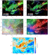 |
Fig. 1 Taurus MC as seen in carbon monoxide, 12CO(J = 1 → 0) and 13CO(J = 1 → 0) emission from Goldsmith et al. (2008), neutral atomic hydrogen (H I) emission from GALFA-H I DR2 (Peek et al. 2018), volume density of hydrogen nuclei (nH) across distances derived from the 3D dust reconstruction in Leike et al. (2020), and hydrogen nuclei column density (NH) derived from the dust optical depth at 353 GHz (τ353) obtained with the Planck observations (Planck Collaboration XI 2014). The contours correspond to NH = 5 × 10²¹, 8 × 10²¹, and 1.25 × 1022 cm−2. The labels in the bottom panel indicate the reference positions for the most prominent objects in Lynds’ catalog of dark nebulae (Lynds 1962) and Barnard’s catalog of dark objects in the sky (Barnard 1927). |
4 Results
4.1 Dust in 2D and 3D
We applied the HOG method to the integrated dust column density derived from the Planck observations (NH) and the nH distribution across distance bins using a Δ = 30′ FWHM derivative kernel, which corresponds to a scale of approximately 1.2 pc at the mean distance to Taurus. To evaluate the impact of random correlation, we also present the results obtained when flipping the NH map vertically and horizontally. The resulting V and rPearson are presented in Fig. 2.
The morphological correlation between these two data sets, as quantified by V, presents maximum values around the distances usually assigned to the Taurus MC. Most of the dust distribution roughly beyond 200 pc shows very small V values. The flipped NH maps produce relatively low values of V with respect to the peak of the values in the original maps, thus suggesting that the effect of chance correlation is negligible.
The concentration of high V around the distance of the MC indicates that most of the integrated NH distribution results from the contributions from the dust in the Taurus MC with negligible input from the material in the background, beyond 200 pc. The V distribution across distances suggests that the morphological matching obtained with the HOG method provides an alternative definition of MC distance. This "morphological distance," understood as the range of line of sight distances that contribute the most to the observed morphology, is complementary to the distance defined using reddening and distances to stars (see, for example, Green et al. 2014; Schlafly et al. 2014; Zucker et al. 2020).
The Pearson correlation coefficient (rPearson) also shows maximum values for the distances around the MC. However, the results of flipping the NH map indicate that rPearson presents large values produced by chance correlation. We interpret these results as indicating that V is less sensitive to chance correlation than the linear correlation quantified by rPearson.
The increase in the values of rPearson roughly matches with the increase in the mean density along the line of sight. In contrast, V appears to be dominated by the density peak around the distance of Taurus. This indicates that the Taurus MC is the dominant feature in the NH map, although it is not the only density structure found along the line of sight.
Figure 3 shows the nH distribution in the slice with the highest V and the V distribution in 5 × 4 blocks, each with an area of roughly 4Δ × 4Δ, for that distance channel. We found a significant correlation between nH and NH toward the regions around the dark clouds B220/L1527 and B211/B213/L1495. There is also significant V toward mostly diffuse regions, for example, in the southeast portion of the map. The highest V is found toward the shell-like feature in the southwest portion of the map, which is not prominent in the near-infrared extinction maps of Taurus (see, for example, Lombardi et al. 2010).
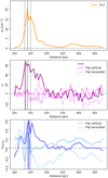 |
Fig. 2 Properties derived from the 3D dust mapping toward the Taurus molecular cloud. Top: Mean volume density of hydrogen nuclei (nH) calculated using Eq. (1). Middle: Projected Rayleigh statistic (V, Eq. (4)) for the integrated dust column density derived from the Planck observations (NH) and the distribution of dust across distance slices in the 3D dust reconstruction. Values of V ≈ 0 correspond to a random orientation between the gradients of the two tracers, thus indicating low morphological correlation. Values of V > 2.87 correspond to the mostly parallel gradient, thus indicating a significant morphological correlation. Bottom: Pearson correlation coefficient (rPearson) between NH and the distribution of dust across distance slices. The solid colored vertical line indicates the distance channel with the maximum V. The faint lines correspond to the chance correlation tests performed by flipping the maps with respect to each other in the vertical and horizontal directions. The black vertical lines indicate the average distance to the Taurus MC and its corresponding confidence interval, as reported in Zucker et al. (2020). |
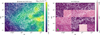 |
Fig. 3 Left: Distribution of the hydrogen volume density (nH), derived from the Leike et al. (2020) 3D dust reconstruction, for the distance channel that shows the highest correlation with the gas column density (NH) derived from the Planck observations, shown by the contours. The white contours correspond to NH = 1, 2, 3, 4, 5, 8, and 12.5 × 1021 cm−2. Right: Distribution of the projected Rayleigh statistic (V, Eq. (4)) in 5 × 4 blocks across the map. The minimum of the color bar is set to 2.87, which is roughly equivalent to a 3σ significance for this indicator of the correlation between the two images. The green disk indicates the derivative kernel size Δ = 30′. |
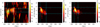 |
Fig. 4 Correlation between the distribution of hydrogen volume density (nH) derived from the Leike et al. (2020) 3D dust reconstruction and the H I, 12CO, and 13CO emission across distances and radial velocities as quantified by the projected Rayleigh statistic (V), as indicated in the color bars to the right of each panel. The lower limit of each color scale is set to the standard deviation of V across the whole distance and velocity range, ςv. The dashed vertical and horizontal lines indicate the minimum and maximum d and υLSR where V is larger than 3ςv. The circle indicates the distance-radial velocity pair with the highest V. The red and blue crosses in the center and left panels indicate the highest radial velocity and nearest distance and the lowest radial velocity and farthest distances with significant V, respectively. |
4.2 Gas and 3D dust
We also applied the HOG method to the H I, 12CO, and 13CO emission and the dust distribution across distance bins using a Δ = 30′ FWHM derivative kernel. The distribution of V across distance slices and radial velocity channels is presented in Fig. 4. The maximum values of V indicate a large correlation in the distribution of the dust and gas tracers. However, there are clear differences between the results obtained for the H I and the two CO isotopologues.
4.2.1 H I and 3D dust
The distribution of V for the H I emission and the 3D dust, shown in the left-hand side panel of Fig. 4, indicates a large spread of relatively high values for a broad range of velocity channels and distances. The highest V values are found in the range 130 ≲ d ≲ 160 pc and 3 ≲ υLSR ≲ 7 km s−1. Yet, we also found high V for a few velocity channels around 5.7 km s−1 at d ≈ 200 pc.
The multiplicity of distances with high V for a particular υLSR implies that the H I emission in a velocity channel results from contributions of gas parcels separated by tens of parsecs. This result is not surprising given the ubiquity of H I and the relatively broad linewidths; around 2 km s−1 and 10 km s−1 for the cold and warm H I phases (see, for example, Kalberla & Kerp 2009). The overlap is particularly acute for υLSR ≈ 5.7 km s−1, where there are high V values at d ≈ 125, 140, and 200 pc.
The top panel in Fig. 5 shows the nH distribution and H I emission for the pair of distance and radial velocity channels with the highest V, indicated by the green circle in the corresponding panel of Fig. 4. The distance with the highest V is found around υLSR ≈ 5.8 km s−1 and d ≈ 145 pc, which indicates that there is a significant correlation between dust in and around the MC and the H I emission. We found, however, that the highest similarity between the tracers comes from regions within Taurus where the increase in nH is associated with a decrease in the H I. Such anticorrelation is expected if we consider that the H I associated with the MC is in the cold phase that is seen as a shadow against the warm phase background, which is known in the literature as H I self-absorption (HISA; Heeschen 1955; Gibson et al. 2000; Wang et al. 2020).
We also found significantly high V for υLSR ≈ 5.8 km s−1 and d ≈ 200 pc. The distribution of dust around that distance, shown in the bottom panel of Fig. 5, corresponds to the H I bright region toward the left-hand side of the map, which most likely corresponds to the background against which the HISA around the B220/L1527 region in Taurus is visible. However, the bright H I filament seen over the more extended emission toward the lower left portion of the map does not have a counterpart in the dust distribution at that distance.
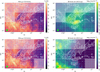 |
Fig. 5 Atomic hydrogen (H I) emission and distribution of the hydrogen volume density (nH) derived from the Leike et al. (2020) 3D dust reconstruction for two radial velocity and distance channels with the highest V, as indicated in Fig. 4. The pseudovectors indicate the orientation of the Tb and nH gradients, shown in white and cyan colors respectively. The translucent mask marks the blocks where V < 2.87, thus indicating areas of negligible morphological correlation. |
4.2.2 CO and 3D dust
The distribution of V for the 12CO and 13CO emission and the 3D dust, shown on the center and right panels of Fig. 4, indicates a concentration of high values in the range 130 ≲ d ≲ 160 pc and 4 ≲ υ ≲ 7 km s−1. In the case of 13CO, the highest V appear closely concentrated around d ≈ 140 pc and υLSR ≈ 6.2 km s−1. In the case of 12CO, the highest V values appear more spread out in velocity and distance. They also show a negative slope distribution in the distance-radial velocity plane that links the highest distances to the lowest velocities and the lowest distances to the highest velocities.
Figure 6 shows the nH distribution and 12CO emission for the distance and radial-velocity channels with the highest V. The similarity in the distribution of both tracers confirms the results of the HOG. Most of the correlation comes from the material within the 5 × 1021 cm−2 (AV ≈ 5) contour, which is around the extinction level usually used to define the Taurus MC in extinction and dust emission observations (see, for example, Cambrésy 1999; Planck Collaboration Int. XXXV 2016). There are, however, small portions of the cloud for which the nH distribution has no counterpart in the 12CO emission in the studied velocity range, particularly toward the lower right corner of the map.
We further explored the negative-slope feature in the center panel of Fig. 4 by dividing the area of the Taurus MC in 4 × 3 blocks and calculating the V distribution across distances and radial velocities. The results toward each block, presented in Fig. 7, indicate that the signal in Fig. 4 is also found in the upper right areas of the Taurus MC, with the largest significance found toward the center of the region. The block with the highest column density, second from left to right in the central row of Fig. 7, shows a discontinuity most likely related to the high extinction limiting the 3D dust reconstruction toward that portion of the cloud. Insofar as the division in blocks does not elucidate the dynamical behavior of each portion of the cloud and is limited by the limited number of independent gradients in each block, we focus on the global trend rather than look for an explanation of the trend for each MC portion.
The global HOG results presented in Fig. 4 indicate that the material at the highest distances is related to the lowest velocities and that material at lower distances is linked to the highest velocities, but it is not limited to these two extremes. This high correlation identified with the HOG method is distributed across the distances and radial velocities between roughly 125 and 175 pc and 4 to 7 km s−1. This distribution implies that the MC’s most distant and closest portions are converging along the line of sight.
The distinctive pattern in V linking the near side of Taurus to its highest 12CO radial velocities and vice versa is slightly distinguishable in the results obtained with 13CO, shown in the right panel of Fig. 4. However, its lower significance limits additional interpretation, as further illustrated in Appendix D.
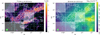 |
Fig. 6 Carbon monoxide (12CO) emission and distribution of the hydrogen volume density (nH) derived from the Leike et al. (2020) 3D dust reconstruction for the radial velocity and distance channels with the highest V, as indicated in Fig. 4. The pseudovectors indicate the orientation of the Tb and nH gradients, shown in white and cyan colors respectively. The translucent mask marks the blocks where V < 2.87, thus indicating areas of negligible morphological correlation. |
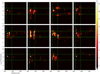 |
Fig. 7 Correlation between the distribution of the hydrogen volume density (nH) derived from the Leike et al. (2020) 3D dust reconstruction and 12CO emission across distances and radial velocities as quantified by the projected Rayleigh statistic (V) for the 4 × 3 regions shown in Fig. 6. The vertical and horizontal dashed lines correspond to the distances and radial velocity ranges defined in Fig. 4. The circle marks the pair of distance and velocity channels with the highest global V, which are presented in Fig. 6. |
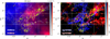 |
Fig. 8 Distribution of the hydrogen volume density (nH) derived from the Leike et al. (2020) 3D dust reconstruction (left) and 12CO emission (right) for the minimum and maximum distance and radial velocity channels with significant correlation, identified by the red and blue crosses in Fig. 4. The maps shown in a blue colormap correspond to the farthest distance and the lowest velocity channels with V > 3ςv, where ςv is the standard deviation of V across the whole distance and velocity range. The maps shown in a red colormap correspond to the nearest distance and the highest velocity channels with V > 3ςv. The yellow and green stars indicate the positions of the young (age < 10 Myr) stellar objects presented in Galli et al. (2019) and young stellar clusters in Luhman (2023), respectively. |
5 Discussion
5.1 Morphology as an indicator of distance
Figure 2 illustrates the agreement between the estimated distance to the Taurus MC and the distances at which the HOG produced the highest correlation, quantified by V. The HOG produces high V when the gradients of two images are mostly parallel. Thus, the finding of high V at the distance of the MC indicates that the dust parcel at d =ĺ40 pc not only has most of the dust along the line of sight, but it is also responsible for most of the features observed in the integrated dust map. This observation is essential for the comparison between the 2D MCs in the literature, which are traditionally in the integrated dust maps, and the novel reconstructions of 3D dust distribution (see, for example, Zucker et al. 2021; Rezaei Kh. & Kainulainen 2022).
The tests of our method applied to the 3D maps of dust reddening from Green et al. (2019) emphasize the importance of the 3D dust reconstruction for the HOG studies, as detailed in Appendix E. The 3D dust maps have the advantage of accounting for the spatial correlations between independent lines of sight, producing a smoother distribution. Moreover, the 3D maps of dust reddening tend to overestimate the cloud distance obtained with the HOG and saturate for distances beyond the dominant feature in the map, as discussed in Appendix E.
We found no significant signal in V at d ≈ 300 pc, corresponding to the backside of the Per-Tau shell identified in Bialy et al. (2021). This lack of correlation indicates that this potential background does not significantly contribute to the integrated dust emission and emphasizes the importance of the 3D dust maps to elucidate this kind of structure surrounding MCs. Being at a relatively high Galactic latitude (b ≈ −14° 5), the integrated dust emission toward Taurus is unlikely to be affected by background contamination. However, this may be critical for clouds at lower b, where the morphological correlation quantified by the HOG can identify what parcel of dust along the LOS is responsible for the integrated emission and what portions of an MC are dominated by different dust parcels along the LOS.
5.2 Dust revealing the presence of cold H I
The anticorrelation between H I emission and nH illustrated in Fig. 5 marks the potential location of HISA in Taurus. Observations of H I in dark clouds in Taurus have previously revealed the presence of H I narrow self-absorption (HINSA) features, suggesting that a significant fraction of the H I in Taurus is located in the cold, well-shielded portions of MCs and is mixed with the molecular gas (Li & Goldsmith 2003; Goldsmith & Li 2005).
Heiner & Vázquez-Semadeni (2013) used the H I spectra to identify HISA and estimate hydrogen volume densities of up to 430 cm−3 within Taurus. This value is at least a factor of two larger than the maximum nH derived from the 3D dust across the MC. This discrepancy can be explained by the limitation of the 3D dust to reconstruct the density toward regions of high extinction.
Given the lack of existing observations of H I absorption around Taurus, just one within 5 of the center of the region (Nguyen et al. 2019), the correlation between the dust and the HISA is a promising path to disentangle the amount of cold H I in and around MCs. We will focus on this topic in the subsequent paper in this series.
5.3 Dynamics of the Taurus MC
The negative slope feature found in the correlation between nH and 12CO emission, shown in the central panel of Fig. 4, indicates that nearby material in Taurus is moving toward the central velocity of the cloud and more distant material is also moving toward it. This motion is consistent with two scenarios. One possibility is rotation on MC scales. The other possibility is the MC is contracting, either by external compression or global collapse.
Taking the cloud as a whole, our results are consistent with a 2.5 km s−1 radial velocity difference more or less aligned with the Galactic plane across roughly 25 pc, that is, a velocity gradient of roughly 0.1 km s−1 pc−1. Meidt et al. (2018) have shown that the gas kinematics on the scale of individual molecular clouds are not entirely dominated by self-gravity but also track a component that originates from orbital motion in the potential of the host galaxy. Pascucci et al. (2015) presents observations of the narrow Na and K absorption lines toward 40 T Tauri stars in the Taurus and found a velocity gradient along the length of the MCs, which the authors suggest is consistent with differential galactic rotation (Imara & Blitz 2011).
Galli et al. (2019) studied the parallax distances and proper motions from Gaia’s Data Release 2 (DR2) and the astrometry obtained with long baseline interferometry (VLBI) for 415 stars toward the Taurus MC. Using the divergence and rotational of stellar proper motions, the authors concluded that the expansion or contraction motions traced by this sample are negligible. They also reported a global rotational velocity of around 1.5 km s−1. However, the results of the HOG indicate a different scenario for the dust and the gas.
Figure 8 shows the nH distribution and the 12CO emission for the extremes of the negative-slope feature identified in Fig. 4 The colors indicate what can be interpreted as a large-scale velocity gradient between υLSR = 4.25 km s−1 and 7.05 km s−1 across Taurus. However, the 12CO emission toward the portion of the MC that shows the HOG signature of compression, as identified in Fig. 7, shows a less clear left-right symmetry. The nH for the two distances associated with the radial velocities shows a mixture of two components, and it is mainly dominated by the nearby one at d = 125 pc.
The comparison between the HOG results and the stellar distances and radial velocities in the Galli et al. (2019) sample, shown on the top panel of Fig. 9, suggest that the stars follow the trend in the gas and dust, albeit with a large scatter. The scatter in the stellar data is explained by the 2.7 km s−1 three-dimensional velocity dispersion reported in Galli et al. (2019), which is close to twice the rotational speed estimated with the proper motions of the stars. The large velocity dispersion with respect to the potential rotational motions suggests that the latter is not dominant in this system.
We also looked for additional indications of converging motions in the Taurus young cluster dynamics identified with Gaia (Esplin & Luhman 2019; Luhman 2023). The bottom panel of Fig. 9 shows in detail the negative-slope pattern identified with the HOG in nH and 12CO emission along with the radial velocities and distances to the young clusters. The roughly 3 km s−1 velocity difference across approximately 80 pc along the LOS identified in the dust and 12CO is not followed by the young stellar clusters. This discrepancy may be related to the current gas dynamics not dominating the young cluster dynamics. Thus, it may indicate the different time scales that coexist within the MC, but does not contradict the compressive motions in the dust and gas.
The Taurus region with the most evident signature of converging motions identified with the HOG method corresponds to the southern portion of the B211/B213 region, which has been identified as an archetypical example of a star-forming filament (Schmalzl et al. 2010; Palmeirim et al. 2013). The Herschel dust emission observations reveal the presence of striations perpendicular to the filament, generally oriented along the magnetic field direction as traced by optical polarization vectors and dust thermal emission (Chapman et al. 2011; Soler 2019; Eswaraiah et al. 2021). These observations have led some authors to suggest that the material may be accreting along the striations onto the main filament (see, for example, Pineda et al. 2022, and references therein). The typical velocities expected for the infalling material in this picture are around 1 km s−1, which is roughly compatible with our estimates, assuming that the dynamics that Palmeirim et al. (2013) study on the plane of the sky are also those that we identified along the LOS.
In a follow-up to Palmeirim et al. (2013), Shimajiri et al. (2019) studied the velocity pattern in the CO emission around the B211/B213 filament and identified the gas motions as the signature of "mass accretion" into that structure. The authors conclusions are based in the emission at υLSR ≈ 6 to 7 km s−1 toward the northeastern edge of the filament and at υLSR ≈ 4–5 km s−1 toward the southern-west edge. These velocities match the results of our analysis, but our analysis suggests that they are produced by the convergence of gas components along the line of sight rather than by gravitational collapse into the filament.
The fact that we found different dynamics in the stars and the combination of dust and gas is most likely related to the origin of the global contraction or compression of Taurus suggested by the HOG results. If the stars, dust, and gas dynamics were dominated by the monolithic collapse toward the bottom of a gravitational potential well, we would expect coherent motion in all the tracers toward a particular location. However, this is not what is obtained by the 3D motions of the stars in Galli et al. (2019) or the results of the HOG. Instead, we found compressive motions in the gas and dust in Taurus but not in the stars, as illustrated in Fig. 9.
Our analysis suggests the convergence of gas components across the whole area of the MC, not continuous convergence in parts of the cloud. This implies that the gas is brought together, rather than collapsing toward the local centers of gravitational collapse. Thus, it is more likely that the convergence is being driven from the exterior of the MC, as with the injection of momentum from supernovae, rather than from the matter in its interior, as would be the case in gravitational collapse. The former scenario gathers the gas while only marginally contributing to the motions of the stars. The latter influences the stars and the gas. Both scenarios can coexist in an MC. Our results indicate that external compression is dominant in the Taurus MC.
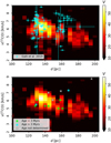 |
Fig. 9 Same as the middle panel of Fig. 4, but for a more limited range of distances and radial velocities and including the radial velocities and distances for the young (age < 10 Myr) stellar objects identified as cluster members in Galli et al. (2019) and young stellar clusters in Luhman (2023). |
5.4 Potential origin of the Taurus MC
The 3D dust maps used in this paper also enable precise constraints on the morphology of feedback-driven shells and super-bubbles. These structures appear as cavities in the interstellar medium and have been identified in the Taurus vicinity and other locations of the solar neighborhood (Pelgrims et al. 2020; Bialy et al. 2021; Marchal & Martin 2023; Foley et al. 2023).
Figure 10 shows the relationship between the 3D position of the Taurus MC and the 3D morphology of the Per-Tau shell (Bialy et al. 2021) and the Local Bubble, whose boundary has been mapped out in Pelgrims et al. (2020) using the 3D dust map of Lallement et al. (2019). Taurus lies at the intersection of these two surfaces, where the Per-Tau shell seems to produce an indentation in the Local Bubble. The near side of the cloud, which is touching the Local Bubble’s surface, travels at higher radial velocities. The far side of the cloud, which is touching the Per-Tau shell, travels at lower radial velocities. Both of these observations strongly suggest that the relation between the radial velocity and distance revealed by the HOG in Fig. 9 is consistent with the formation of the Taurus MC as a result of large-scale gas compression via a "snowplow" effect produced by the SN-driven expansion of two superbubbles (see, for example, Inutsuka et al. 2015; Dawson 2013).
The colliding shells scenario is consistent with the sheetlike morphology of Taurus in 3D dust at lower densities, as identified in Zucker et al. (2021). The shock-compressed layers are possibly the origin of the network of filamentary structures embedded within the cloud at higher densities (Arzoumanian et al. 2013). These structures appear to evolve independently, as suggested by the proper motions of the stellar associations in Taurus (Roccatagliata et al. 2020), and give rise to the young (a few megayears old) stellar population (Luhman 2018). Although the young stellar population does not rule out an MC origin by gravitational contraction, it matches what is expected if the MC had only formed recently due to the bubble collision, whereas the presence of an older population, for example, clusters with ages around 10 Myr, would have been inconsistent with this scenario.
6 Conclusions
We used the machine vision method HOG (Soler et al. 2019) to study the relation between the 3D dust reconstruction presented in Leike et al. (2020) and the H I, 12CO, and 13CO emission toward the Taurus MC. We showed that the morphological correlation quantified by the HOG provides a robust estimate of the distance to the MC by determining the dust parcel along the LOS that contributes the most to the observed distribution in integrated dust extinction or emission maps. Thus, the HOG provides a powerful tool to determine distances to the features identified in 2D maps and disentangle the contributions of different dust parcels to the integrated maps.
We identified the anticorrelation between the mass traced by the 3D dust reconstruction and the H I emission toward the Taurus MC. We interpreted this result as the effect of the cold H I associated with the MC. We devote a follow-up paper to a detailed study of the H I within Taurus.
We also found the potential signature of the converging motions in the HOG correlation between the 3D dust and 12CO. The imprint of these motions is strongest toward the region around the star-forming filament B211/3.
The converging motion signature in the 3D dust and 12CO differs from the potential rotation signatures found in the proper motions of the stars in Taurus (Galli et al. 2019). However, this discrepancy is not in tension with our results for two main reasons. First, the velocity of the potential rotational motion reported in Galli et al. (2019) is below the 3D velocity dispersion of the stars, thus indicating that the rotation is not dominant in this system. Second, the dynamics of the dust and gas are not necessarily the same as those of the stars. The fact that we are finding converging motions in the gas and not in the stars can be interpreted as an indication that these are not dominated by a monolithic gravitational collapse, which would affect both the stars and the ISM, but rather by a large-scale shock that pushes and gathers the lower-density ISM.
The results of the HOG are consistent with the potential origin of the Taurus MC as the result of material compression by the expansion of the Local Bubble and the Per-Tau shell. This dynamic imprint is a concrete observable that can be targeted in the analysis of numerical simulations and their associated synthetic observations to study the prevalence of this MC formation scenario. Also, as more superbubbles are mapped out in 3D across the solar neighborhood, the HOG technique presented here provides an opportunity to test MC formation mechanisms over a larger statistical sample.
We used the HOG method to map the distances revealed by dust into the radial velocity sampled by the gas tracers, revealing various aspects of one of the most studied MCs. However, the correlation between gas tracers and 3D dust is just one of the MC characteristics that can be studied using the HOG and other novel statistical tools. We devote two forthcoming papers to studying the cold atomic hydrogen in and around the Taurus and its relation with the interstellar magnetic field.
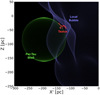 |
Fig. 10 Locations of the Taurus MC, Local Bubble, and the Per-Tau shell in an X-Z projection in heliocentric Galactic Cartesian coordinates. The X-axis (X′) has been rotated counterclockwise by θ = 33° to show the best view of the intersection of the two shells. The red points correspond to the 3D model of the dense gas in Taurus presented in Zucker et al. (2021), based on the 3D dust reconstruction presented in Leike et al. (2020). The Local Bubble surface, shown in purple, corresponds to the structure identified in Pelgrims et al. (2020), based on the 3D dust reconstruction presented in Lallement et al. (2019). The Per-Tau shell surface, shown in green, corresponds to the structure identified in Bialy et al. (2021), based on the 3D dust reconstruction presented in Leike et al. (2020). Taurus lies at the intersection of the two surfaces. |
Acknowledgements
The European Research Council funds J.D.S. via the ERC Synergy Grant "ECOGAL - Understanding our Galactic ecosystem: From the disk of the Milky Way to the formation sites of stars and planets" (project ID 855130). C.Z. acknowledges support for this work through the National Aeronautics and Space Administration (NASA) Hubble Fellowship grant #HST-HF2-51498.001 awarded by the Space Telescope Science Institute (STScl), operated by the Association of Universities for Research in Astronomy, Inc., for NASA, under contract NAS5-26555. P.F.G. acknowledges this research was conducted partly at the Jet Propulsion Laboratory, which the California Institute of Technology operates under NASA contract 80NM0018D0004. R.S.K. and S.C.O.G. acknowledge funding from the Deutsche Forschungsgemeinschaft (DFG) via the Collaborative Research Center (SFB 881, Project-ID 138713538) "The Milky Way System" (subprojects A1, B1, B2, and B8) and from the Heidelberg cluster of excellence (EXC 2181 - 390900948) "STRUCTURES: a unifying approach to emergent phenomena in the physical world, mathematics, and complex data", funded by the German Excellence Strategy. We thank the anonymous referee for the thorough review and appreciate the suggestions that helped us improve this manuscript. Part of the crucial discussions that led to this work took part under the program Milky-Way-Gaia of the PSI2 project funded by the IDEX Paris-Saclay, ANR-11-IDEX-0003-02. JDS thanks the following people who helped with their encouragement and conversation: Henrik Beuther, Jonas Syed, Robert Benjamin, Daniel Seifried, Rosine Lallement, Sara Rezaei Kh., and Sharon Meidt. This research has made use of the SIMBAD database, operated at CDS, Strasbourg, France. The computations for this work were made at the Max-Planck Institute for Astronomy (MPIA) astro-node servers. Software: astropy (Astropy Collaboration 2018), SciPy (Virtanen et al. 2020), astroHOG (Soler 2020).
Appendix A Statistical significance of the HOG results
The results of the HOG analysis are presented in terms of the projected Rayleigh statistic (V), presented in Eq. (4) (Jow et al. 2018). In the following sections, we evaluate the effect of the uncertainties in the 3D dust and emission maps and the impact of chance correlations.
A.1 Error propagation
The H I and CO emission maps have uncertainties associated with the sensitivity of the instrument used to obtain them. The 3D dust reconstruction has uncertainties related to reconstructing a continuous distribution based on discrete sampling. We evaluated the effect of both uncertainties in the values of V using Monte Carlo sampling.
For each velocity channel map and nH slice, we generated ten Monte Carlo realizations with an amplitude equal to the 1-σ uncertainty in each data set. The results are 100 values of V per distance and radial-velocity pair. We computed the mean value  , which we reported in the main body of this paper, and the standard deviation around this value, σv, which we report in Fig. A.1.
We found that the values of σv are comparable to the 1-σ absolute significance estimates for V introduced in Sect. 3. The maximum values of σv are around V ≈ 1.64, which correspond to the rejection of a uniform distribution of orientations between the gradients with a probability of 5% (Batschelet 1972). Thus, we conclude that the uncertainties in the emission PPV cubes and nH are not systematically biasing the results of our analysis.
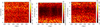 |
Fig. A.1 Dispersion in the projected Rayleigh statistic (V) between the nH and the H I, 12CO, 13CO emission across distances and velocity channels estimated using Monte Carlo simulations of the input data. |
A.2 impact of chance correlation
Two independent 2D scalar fields, like the dust slices or gas emission velocity channels compared in this paper, can show some correlation due to the random alignment between their features, or chance correlation (see, appendix B in Soler et al. 2019). We tested the impact of chance correlation in the values of V using the same atomic and molecular emission PPV cubes but flipping the nH cube.
The results obtained for H I and 3D dust, presented in Fig. A.2, indicate a relatively high chance correlation between these two tracers. The difference between the V maximum values obtained with the original data and the two flipping tests are within 20% of each other, thus setting tight constraints on the significance of the H I to 3D dust correlation over the whole radial velocity and distance range. However, the flipping tests confirm that the high V values obtained around the distance of the Taurus MC are not the product of chance correlation.
The results obtained for the two CO isotopologues and 3D dust, presented in Fig. A.3 and Fig. A.4, show a lower chance correlation than in the H I study. This is expected given the more limited coverage of CO in the maps in relation to the almost ubiquitous H I. The maximum V values in the original data are almost double those obtained in the flipping tests. The V distribution across distances and radial velocities is also very different in the flipping test. It demonstrates that the patterns interpreted in the main body of this paper are not the product of chance correlation.
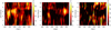 |
Fig. A.2 Tests of change correlation between the H I emission and the 3D dust reconstruction for a Δ = 30′ FWHM derivative kernel and a I >σI mask. Left. Original maps. Center. Flipping the 3D dust cube in the horizontal direction. Right. Flipping the 3D dust cube in the vertical and the horizontal directions. |
Appendix B Angular resolution tests
Throughout this paper, we have presented the results of the HOG analysis using the input observations at their native resolution. This choice is justified because the computation of the gradients employing the Gaussian derivatives convolves the images to the common scale set by the size of the derivative kernel. There is, however, an increase in the S/N if the input data are convolved to a common angular resolution larger than the beam size before computing the HOG. This change in S/N potentially produces different results of the HOG analysis, either by modifying the low-signal regions that are masked or by setting a different mean in the Monte Carlo realizations. In this appendix, we present the results obtained when smoothing the maps to a common angular resolution before computing the HOG.
Figure B.1 presents the results of the HOG analysis for the 12CO emission and the 3D dust using three different combinations of the input maps: one in which both have their native angular resolution, one in which the 12CO is smoothed with a 24.′6 FWHM kernel, and one in which both maps are smoothed with this kernel. The 24.′6 kernel width corresponds to 1pc at the mean distance to Taurus In the HOG computation, we employed a 30.′0 FWHM derivative kernel and a S/N> 3 mask The smoothing of the 12CO input data produces higher maximum values of V and high V in distance and velocity channel pairs that are not statistically significant with the raw input data This is most likely due to the reduction of the masked regions in the smoothed maps due to the increase in S/N for the lower-resolution data. The 3ςv distance and velocity ranges are identical in the three cases. The changes in the distribution of V across distance and velocity channels do not significantly affect the main trend reported in the paper.
Figure B.2 presents the results of the HOG analysis for the 12CO emission and the 3D dust using the same three different combinations of the input map smoothing, but with the HOG computed using the Monte Carlo realizations introduced in App. A instead of masking. The results of this test indicate an increase in V of around 10%, but the same global distribution of V across distance and velocity channels in the three cases. This confirms that the differences found between the three combinations of input maps in Fig. B.1 are produced by the masking. The 3σv distance and velocity ranges are essentially identical in the three cases, just with a slight change in the furthest distance channel due to the general increase in the V. However, the global trend within the 3σv range is unchanged. These results indicate that the initial smoothing does not significantly affect the results of our analysis and supports our choice of Monte Carlo realizations instead of masking.
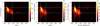 |
Fig. B.1 Correlation between the distribution of hydrogen volume density (nH) derived from the Leike et al. (2020) 3D dust reconstruction and 12CO emission across distances and radial velocities as quantified by the projected Rayleigh statistic (V) using a 30.′0 FWHM derivative kernel. The three panels correspond to three different input data as follows. Left. 3D dust and 12CO at their native angular resolution, 6.′87 and 45", respectively. Center. 3D dust at its native angular resolution and 12CO smoothed to a 24.′6 FWHM resolution. Right. 3D dust and 12CO smoothed to a 24.′6 FWHM resolution. In all three cases, regions with S/N < 3 are excluded from the analysis. |
Appendix C Masking tests
Traditionally, the Taurus MC was defined through the visual extinction AV (see, for example, Cambrésy 1999). Here, we discuss the results obtained when applying the HOG only to the portions of the Taurus MC within the regions defined by cuts in AV. Fig. C.1 shows that the optically thick regions in the V band, AV > 1.0, maintain the trends described in the main body of this paper, which are the high correlation between H I and 3D dust at the distance of Taurus and the high correlation between 12CO and 3D implying that the near side of the cloud is moving at higher velocities and the far side is moving at lower velocities. The same patterns are lost with a higher extinction cut, AV > 3.0, as shown in Fig. C.2. The main reason for this loss in signal is the lack of independent gradient vectors, which is reflected in the lower V values. At this relatively high extinction, the 3D dust reconstruction also saturates its density values, and the gradients used to trace its correlation with the gas emission are less meaningful.
Appendix D Block averaging
For the sake of completeness, we report the results of the HOG comparison between 3D dust and H I and 13CO in 4 × 3 blocks across the Taurus MCs in Fig. D.1 and Fig. D.2, respectively. In the case of 13CO and 3D dust, the panel corresponding to the vicinity of the B211/B213 region displays the pattern linking the near side of the MC moving at higher velocities and the far side moving at lower velocities that was reported for 12CO and 3D dust in the main body of the paper. However, the levels of significance are low and limit any further interpretation.
Appendix E Test using 3D extinction maps
To contrast the results obtained with the nH reconstructions, we also applied the HOG analysis to the 3D maps of dust reddening, E(B – V), based on Gaia parallaxes and stellar photometry from Pan-STARRS 1 and 2MASS (Green et al. 2019). The main difference between the 3D extinction maps and the 3D dust reconstructions is that the former corresponds to a cumulative quantity, which saturates to a maximum value. They also do not account for the spatial correlations between contiguous lines of sight. Still, we highlight the importance of the 3D density reconstruction for our results by computing the HOG with the 3D extinction maps toward Taurus.
Figure E.1 shows the results of the correlation between the H I, 12CO, and 13CO emission and the dust reddening along the line of sight toward the Taurus MC. The HOG method consistently recovers the spatial correlation between the gas emission and the extinction, but the distance where the increase in V indicates the presence of the MC is larger than that of Taurus. This fact is related to the lack of spatial correlation for contiguous pixels in the extinction maps and the cumulative nature of extinction: a meaningful gradient only appears when enough contiguous pixels are correlated by the increase in the number of background stars. The cumulative nature of the 3D extinction maps also implies that they are not sensitive to the structure behind the dominant dust feature in the map, which can only be recovered as a differential quantity between extinction slabs around the line of sight. Thus, the results reported in the main body of this paper are only possible thanks to the reconstruction of a smooth distribution both in the plane of the sky and along the line of sight in the 3D density maps.
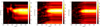 |
Fig. E.1 Correlation between the dust extinction across distances (Green et al. 2019) and H I emission across distances and velocity channels as quantified by the projected Rayleigh statistic (V) and the Pearson correlation coefficient (rPearson). |
References
- Anders, F., Khalatyan, A., Chiappini, C., et al. 2019, A&A, 628, A94 [NASA ADS] [CrossRef] [EDP Sciences] [Google Scholar]
- Arzoumanian, D., André, P., Peretto, N., & Könyves, V. 2013, A&A, 553, A119 [NASA ADS] [CrossRef] [EDP Sciences] [Google Scholar]
- Astropy Collaboration (Price-Whelan, A. M., et al.) 2018, AJ, 156, 123 [Google Scholar]
- Barnard, E. E. 1919, ApJ, 49, 1 [NASA ADS] [CrossRef] [Google Scholar]
- Barnard, E. E. 1927, Catalogue of 349 dark objects in the sky (Chicago: University of Chicago Press) [Google Scholar]
- Batschelet, E. 1972, Recent Statistical Methods for Orientation Data, 262, 61 [Google Scholar]
- Bialy, S., Zucker, C., Goodman, A., et al. 2021, ApJ, 919, L5 [NASA ADS] [CrossRef] [Google Scholar]
- Cambrésy, L. 1999, A&A, 345, 965 [NASA ADS] [Google Scholar]
- Chapman, N. L., Goldsmith, P. F., Pineda, J. L., et al. 2011, ApJ, 741, 21 [NASA ADS] [CrossRef] [Google Scholar]
- Chen, B. Q., Huang, Y., Yuan, H. B., et al. 2019, MNRAS, 483, 4277 [Google Scholar]
- Chevance, M., Krumholz, M. R., McLeod, A. F., et al. 2022, arXiv e-prints [arXiv:2203.09570] [Google Scholar]
- Cox, D. P., & Reynolds, R. J. 1987, ARA&A, 25, 303 [NASA ADS] [CrossRef] [Google Scholar]
- Dawson, J. R. 2013, PASA, 30, e025 [NASA ADS] [CrossRef] [Google Scholar]
- Dharmawardena, T. E., Bailer-Jones, C. A. L., Fouesneau, M., et al. 2023, MNRAS, 519, 228 [Google Scholar]
- Dobbs, C. L., Krumholz, M. R., Ballesteros-Paredes, J., et al. 2014, in Protostars and Planets VI, eds. H. Beuther, R. S. Klessen, C. P. Dullemond, & T. Henning (Tucson: University of Arizona Press), 3 [Google Scholar]
- Draine, B. T. 2011, Physics of the Interstellar and Intergalactic Medium (Princeton University Press) [Google Scholar]
- Durand, D., & Greenwood, J. A. 1958, J. Geol., 66, 229 [Google Scholar]
- Erickson, N. R., Grosslein, R. M., Erickson, R. B., & Weinreb, S. 1999, IEEE Trans. Microwave Theory Tech., 47, 2212 [Google Scholar]
- Esplin, T. L., & Luhman, K. L. 2019, AJ, 158, 54 [Google Scholar]
- Eswaraiah, C., Li, D., Furuya, R. S., et al. 2021, ApJ, 912, L27 [NASA ADS] [CrossRef] [Google Scholar]
- Ferrière, K. M. 2001, Rev. Modern Phys., 73, 1031 [CrossRef] [Google Scholar]
- Foley, M. M., Goodman, A., Zucker, C., et al. 2023, ApJ, 947, 66 [NASA ADS] [CrossRef] [Google Scholar]
- Gaia Collaboration (Brown, A. G. A., et al.) 2018, A&A, 616, A1 [NASA ADS] [CrossRef] [EDP Sciences] [Google Scholar]
- Galli, P. A. B., Loinard, L., Bouy, H., et al. 2019, A&A, 630, A137 [NASA ADS] [CrossRef] [EDP Sciences] [Google Scholar]
- Gibson, S. J., Taylor, A. R., Higgs, L. A., & Dewdney, P. E. 2000, ApJ, 540, 851 [NASA ADS] [CrossRef] [Google Scholar]
- Goldsmith, P. F., & Li, D. 2005, ApJ, 622, 938 [NASA ADS] [CrossRef] [Google Scholar]
- Goldsmith, P. F., Heyer, M., Narayanan, G., et al. 2008, ApJ, 680, 428 [Google Scholar]
- Górski, K. M., Hivon, E., Banday, A. J., et al. 2005, ApJ, 622, 759 [Google Scholar]
- Green, G. M., Schlafly, E. F., Finkbeiner, D. P., et al. 2014, ApJ, 783, 114 [NASA ADS] [CrossRef] [Google Scholar]
- Green, G. M., Schlafly, E., Zucker, C., Speagle, J. S., & Finkbeiner, D. 2019, ApJ, 887, 93 [NASA ADS] [CrossRef] [Google Scholar]
- Heeschen, D. S. 1955, ApJ, 121, 569 [NASA ADS] [CrossRef] [Google Scholar]
- Heiner, J. S., & Vázquez-Semadeni, E. 2013, MNRAS, 429, 3584 [CrossRef] [Google Scholar]
- Heyer, M., & Dame, T. M. 2015, ARA&A, 53, 583 [Google Scholar]
- Heyer, M., Soler, J. D., & Burkhart, B. 2020, MNRAS, 496, 4546 [NASA ADS] [CrossRef] [Google Scholar]
- Imara, N., & Blitz, L. 2011, ApJ, 732, 78 [NASA ADS] [CrossRef] [Google Scholar]
- Inutsuka, S.-I., Inoue, T., Iwasaki, K., & Hosokawa, T. 2015, A&A, 580, A49 [NASA ADS] [CrossRef] [EDP Sciences] [Google Scholar]
- Jow, D. L., Hill, R., Scott, D., et al. 2018, MNRAS, 474, 1018 [NASA ADS] [CrossRef] [Google Scholar]
- Joy, A. H. 1945, ApJ, 102, 168 [Google Scholar]
- Kaiser, N., Aussel, H., Burke, B. E., et al. 2002, SPIE Conf. Ser., 4836, 154 [Google Scholar]
- Kalberla, P. M. W., & Kerp, J. 2009, ARA&A, 47, 27 [NASA ADS] [CrossRef] [Google Scholar]
- Kenyon, S. J., & Hartmann, L. 1995, ApJS, 101, 117 [Google Scholar]
- Kenyon, S. J., Gómez, M., & Whitney, B. A. 2008, Low Mass Star Formation in the Taurus-Auriga Clouds, ed. B. Reipurth, 405 [Google Scholar]
- Klessen, R. S., & Glover, S. C. O. 2016, Star Formation in Galaxy Evolution: Connecting Numerical Models to Reality, Saas-Fee Advanced Course (Springer-Verlag), 43, 85 [NASA ADS] [CrossRef] [Google Scholar]
- Knollmüller, J., & Enßlin, T. A. 2018, arXiv e-prints [arXiv:1812.04403] [Google Scholar]
- Lallement, R., Capitanio, L., Ruiz-Dern, L., et al. 2018, A&A, 616, A132 [NASA ADS] [CrossRef] [EDP Sciences] [Google Scholar]
- Lallement, R., Babusiaux, C., Vergely, J. L., et al. 2019, A&A, 625, A135 [NASA ADS] [CrossRef] [EDP Sciences] [Google Scholar]
- Leike, R. H., & Enßlin, T. A. 2019, A&A, 631, A32 [NASA ADS] [CrossRef] [EDP Sciences] [Google Scholar]
- Leike, R. H., Glatzle, M., & Enßlin, T. A. 2020, A&A, 639, A138 [NASA ADS] [CrossRef] [EDP Sciences] [Google Scholar]
- Li, D., & Goldsmith, P. F. 2003, ApJ, 585, 823 [NASA ADS] [CrossRef] [Google Scholar]
- Lilley, A. E. 1955, ApJ, 121, 559 [NASA ADS] [CrossRef] [Google Scholar]
- Lombardi, M., Lada, C. J., & Alves, J. 2010, A&A, 512, A67 [NASA ADS] [CrossRef] [EDP Sciences] [Google Scholar]
- Luhman, K. L. 2018, AJ, 156, 271 [Google Scholar]
- Luhman, K. L. 2023, AJ, 165, 37 [NASA ADS] [CrossRef] [Google Scholar]
- Lynds, B. T. 1962, ApJS, 7, 1 [NASA ADS] [CrossRef] [Google Scholar]
- Marchal, A., & Martin, P. G. 2023, ApJ, 942, 70 [NASA ADS] [CrossRef] [Google Scholar]
- Martin, P. G., Roy, A., Bontemps, S., et al. 2012, ApJ, 751, 28 [NASA ADS] [CrossRef] [Google Scholar]
- Meidt, S. E., Leroy, A. K., Rosolowsky, E., et al. 2018, ApJ, 854, 100 [NASA ADS] [CrossRef] [Google Scholar]
- Miville-Deschênes, M.-A., Murray, N., & Lee, E. J. 2017, ApJ, 834, 57 [Google Scholar]
- Narayanan, G., Heyer, M. H., Brunt, C., et al. 2008, ApJS, 177, 341 [NASA ADS] [CrossRef] [Google Scholar]
- Nguyen, H., Dawson, J. R., Lee, M.-Y., et al. 2019, ApJ, 880, 141 [NASA ADS] [CrossRef] [Google Scholar]
- Palmeirim, P., André, P., Kirk, J., et al. 2013, A&A, 550, A38 [NASA ADS] [CrossRef] [EDP Sciences] [Google Scholar]
- Pascucci, I., Edwards, S., Heyer, M., et al. 2015, ApJ, 814, 14 [Google Scholar]
- Peek, J. E. G., Babler, B. L., Zheng, Y., et al. 2018, ApJS, 234, 2 [Google Scholar]
- Pelgrims, V., Ferrière, K., Boulanger, F., Lallement, R., & Montier, L. 2020, A&A, 636, A17 [EDP Sciences] [Google Scholar]
- Pineda, J. E., Arzoumanian, D., André, P., et al. 2022, arXiv e-prints [arXiv:2205.03935] [Google Scholar]
- Planck Collaboration XXIV. 2011, A&A, 536, A24 [NASA ADS] [CrossRef] [EDP Sciences] [Google Scholar]
- Planck Collaboration XI. 2014, A&A, 571, A11 [NASA ADS] [CrossRef] [EDP Sciences] [Google Scholar]
- Planck Collaboration Int. XXXV. 2016, A&A, 586, A138 [NASA ADS] [CrossRef] [EDP Sciences] [Google Scholar]
- Rebull, L. M., Padgett, D. L., McCabe, C. E., et al. 2010, ApJS, 186, 259 [NASA ADS] [CrossRef] [Google Scholar]
- Rezaei Kh. S., & Kainulainen, J. 2022, ApJ, 930, L22 [NASA ADS] [CrossRef] [Google Scholar]
- Roccatagliata, V., Franciosini, E., Sacco, G. G., Randich, S., & Sicilia-Aguilar, A. 2020, A&A, 638, A85 [NASA ADS] [CrossRef] [EDP Sciences] [Google Scholar]
- Roman-Duval, J., Heyer, M., Brunt, C. M., et al. 2016, ApJ, 818, 144 [NASA ADS] [CrossRef] [Google Scholar]
- Rosolowsky, E., Hughes, A., Leroy, A. K., et al. 2021, MNRAS, 502, 1218 [NASA ADS] [CrossRef] [Google Scholar]
- Sanders, W. T., Kraushaar, W. L., Nousek, J. A., & Fried, P. M. 1977, ApJ, 217, L87 [Google Scholar]
- Schlafly, E. F., Green, G., Finkbeiner, D. P., et al. 2014, ApJ, 786, 29 [NASA ADS] [CrossRef] [Google Scholar]
- Schmalzl, M., Kainulainen, J., Quanz, S. P., et al. 2010, ApJ, 725, 1327 [NASA ADS] [CrossRef] [Google Scholar]
- Shimajiri, Y., André, P., Palmeirim, P., et al. 2019, A&A, 623, A16 [NASA ADS] [CrossRef] [EDP Sciences] [Google Scholar]
- Skrutskie, M. F., Cutri, R. M., Stiening, R., et al. 2006, AJ, 131, 1163 [NASA ADS] [CrossRef] [Google Scholar]
- Snowden, S. L., Koutroumpa, D., Kuntz, K. D., Lallement, R., & Puspitarini, L. 2015, ApJ, 806, 120 [NASA ADS] [CrossRef] [Google Scholar]
- Soler, J. D. 2019, A&A, 629, A96 [NASA ADS] [CrossRef] [EDP Sciences] [Google Scholar]
- Soler, J. D. 2020, Astrophysics Source Code Library [record ascl:2003.013] [Google Scholar]
- Soler, J. D., Hennebelle, P., Martin, P. G., et al. 2013, ApJ, 774, 128 [Google Scholar]
- Soler, J. D., Beuther, H., Rugel, M., et al. 2019, A&A, 622, A166 [NASA ADS] [CrossRef] [EDP Sciences] [Google Scholar]
- Tchernyshyov, K., & Peek, J. E. G. 2017, AJ, 153, 8 [Google Scholar]
- Ungerechts, H., & Thaddeus, P. 1987, ApJS, 63, 645 [Google Scholar]
- Vergely, J. L., Lallement, R., & Cox, N. L. J. 2022, A&A, 664, A174 [NASA ADS] [CrossRef] [EDP Sciences] [Google Scholar]
- Virtanen, P., Gommers, R., Oliphant, T. E., et al. 2020, Nat. Methods, 17, 261 [Google Scholar]
- Wang, Y., Bihr, S., Beuther, H., et al. 2020, A&A, 634, A139 [NASA ADS] [CrossRef] [EDP Sciences] [Google Scholar]
- Wright, E. L., Eisenhardt, P. R. M., Mainzer, A. K., et al. 2010, AJ, 140, 1868 [Google Scholar]
- Zucker, C., Speagle, J. S., Schlafly, E. F., et al. 2020, A&A, 633, A51 [NASA ADS] [CrossRef] [EDP Sciences] [Google Scholar]
- Zucker, C., Goodman, A., Alves, J., et al. 2021, ApJ, 919, 35 [NASA ADS] [CrossRef] [Google Scholar]
- Zucker, C., Goodman, A. A., Alves, J., et al. 2022, Nature, 601, 334 [NASA ADS] [CrossRef] [Google Scholar]
All Figures
|
Fig. 1 Taurus MC as seen in carbon monoxide, 12CO(J = 1 → 0) and 13CO(J = 1 → 0) emission from Goldsmith et al. (2008), neutral atomic hydrogen (H I) emission from GALFA-H I DR2 (Peek et al. 2018), volume density of hydrogen nuclei (nH) across distances derived from the 3D dust reconstruction in Leike et al. (2020), and hydrogen nuclei column density (NH) derived from the dust optical depth at 353 GHz (τ353) obtained with the Planck observations (Planck Collaboration XI 2014). The contours correspond to NH = 5 × 10²¹, 8 × 10²¹, and 1.25 × 1022 cm−2. The labels in the bottom panel indicate the reference positions for the most prominent objects in Lynds’ catalog of dark nebulae (Lynds 1962) and Barnard’s catalog of dark objects in the sky (Barnard 1927). |
| In the text | |
|
Fig. 2 Properties derived from the 3D dust mapping toward the Taurus molecular cloud. Top: Mean volume density of hydrogen nuclei (nH) calculated using Eq. (1). Middle: Projected Rayleigh statistic (V, Eq. (4)) for the integrated dust column density derived from the Planck observations (NH) and the distribution of dust across distance slices in the 3D dust reconstruction. Values of V ≈ 0 correspond to a random orientation between the gradients of the two tracers, thus indicating low morphological correlation. Values of V > 2.87 correspond to the mostly parallel gradient, thus indicating a significant morphological correlation. Bottom: Pearson correlation coefficient (rPearson) between NH and the distribution of dust across distance slices. The solid colored vertical line indicates the distance channel with the maximum V. The faint lines correspond to the chance correlation tests performed by flipping the maps with respect to each other in the vertical and horizontal directions. The black vertical lines indicate the average distance to the Taurus MC and its corresponding confidence interval, as reported in Zucker et al. (2020). |
| In the text | |
|
Fig. 3 Left: Distribution of the hydrogen volume density (nH), derived from the Leike et al. (2020) 3D dust reconstruction, for the distance channel that shows the highest correlation with the gas column density (NH) derived from the Planck observations, shown by the contours. The white contours correspond to NH = 1, 2, 3, 4, 5, 8, and 12.5 × 1021 cm−2. Right: Distribution of the projected Rayleigh statistic (V, Eq. (4)) in 5 × 4 blocks across the map. The minimum of the color bar is set to 2.87, which is roughly equivalent to a 3σ significance for this indicator of the correlation between the two images. The green disk indicates the derivative kernel size Δ = 30′. |
| In the text | |
|
Fig. 4 Correlation between the distribution of hydrogen volume density (nH) derived from the Leike et al. (2020) 3D dust reconstruction and the H I, 12CO, and 13CO emission across distances and radial velocities as quantified by the projected Rayleigh statistic (V), as indicated in the color bars to the right of each panel. The lower limit of each color scale is set to the standard deviation of V across the whole distance and velocity range, ςv. The dashed vertical and horizontal lines indicate the minimum and maximum d and υLSR where V is larger than 3ςv. The circle indicates the distance-radial velocity pair with the highest V. The red and blue crosses in the center and left panels indicate the highest radial velocity and nearest distance and the lowest radial velocity and farthest distances with significant V, respectively. |
| In the text | |
|
Fig. 5 Atomic hydrogen (H I) emission and distribution of the hydrogen volume density (nH) derived from the Leike et al. (2020) 3D dust reconstruction for two radial velocity and distance channels with the highest V, as indicated in Fig. 4. The pseudovectors indicate the orientation of the Tb and nH gradients, shown in white and cyan colors respectively. The translucent mask marks the blocks where V < 2.87, thus indicating areas of negligible morphological correlation. |
| In the text | |
|
Fig. 6 Carbon monoxide (12CO) emission and distribution of the hydrogen volume density (nH) derived from the Leike et al. (2020) 3D dust reconstruction for the radial velocity and distance channels with the highest V, as indicated in Fig. 4. The pseudovectors indicate the orientation of the Tb and nH gradients, shown in white and cyan colors respectively. The translucent mask marks the blocks where V < 2.87, thus indicating areas of negligible morphological correlation. |
| In the text | |
|
Fig. 7 Correlation between the distribution of the hydrogen volume density (nH) derived from the Leike et al. (2020) 3D dust reconstruction and 12CO emission across distances and radial velocities as quantified by the projected Rayleigh statistic (V) for the 4 × 3 regions shown in Fig. 6. The vertical and horizontal dashed lines correspond to the distances and radial velocity ranges defined in Fig. 4. The circle marks the pair of distance and velocity channels with the highest global V, which are presented in Fig. 6. |
| In the text | |
|
Fig. 8 Distribution of the hydrogen volume density (nH) derived from the Leike et al. (2020) 3D dust reconstruction (left) and 12CO emission (right) for the minimum and maximum distance and radial velocity channels with significant correlation, identified by the red and blue crosses in Fig. 4. The maps shown in a blue colormap correspond to the farthest distance and the lowest velocity channels with V > 3ςv, where ςv is the standard deviation of V across the whole distance and velocity range. The maps shown in a red colormap correspond to the nearest distance and the highest velocity channels with V > 3ςv. The yellow and green stars indicate the positions of the young (age < 10 Myr) stellar objects presented in Galli et al. (2019) and young stellar clusters in Luhman (2023), respectively. |
| In the text | |
|
Fig. 9 Same as the middle panel of Fig. 4, but for a more limited range of distances and radial velocities and including the radial velocities and distances for the young (age < 10 Myr) stellar objects identified as cluster members in Galli et al. (2019) and young stellar clusters in Luhman (2023). |
| In the text | |
|
Fig. 10 Locations of the Taurus MC, Local Bubble, and the Per-Tau shell in an X-Z projection in heliocentric Galactic Cartesian coordinates. The X-axis (X′) has been rotated counterclockwise by θ = 33° to show the best view of the intersection of the two shells. The red points correspond to the 3D model of the dense gas in Taurus presented in Zucker et al. (2021), based on the 3D dust reconstruction presented in Leike et al. (2020). The Local Bubble surface, shown in purple, corresponds to the structure identified in Pelgrims et al. (2020), based on the 3D dust reconstruction presented in Lallement et al. (2019). The Per-Tau shell surface, shown in green, corresponds to the structure identified in Bialy et al. (2021), based on the 3D dust reconstruction presented in Leike et al. (2020). Taurus lies at the intersection of the two surfaces. |
| In the text | |
|
Fig. A.1 Dispersion in the projected Rayleigh statistic (V) between the nH and the H I, 12CO, 13CO emission across distances and velocity channels estimated using Monte Carlo simulations of the input data. |
| In the text | |
|
Fig. A.2 Tests of change correlation between the H I emission and the 3D dust reconstruction for a Δ = 30′ FWHM derivative kernel and a I >σI mask. Left. Original maps. Center. Flipping the 3D dust cube in the horizontal direction. Right. Flipping the 3D dust cube in the vertical and the horizontal directions. |
| In the text | |
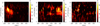 |
Fig. A.3 Same as Fig. A.2, but for 12CO. |
| In the text | |
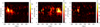 |
Fig. A.4 Same as Fig. A.2, but for 13CO. |
| In the text | |
|
Fig. B.1 Correlation between the distribution of hydrogen volume density (nH) derived from the Leike et al. (2020) 3D dust reconstruction and 12CO emission across distances and radial velocities as quantified by the projected Rayleigh statistic (V) using a 30.′0 FWHM derivative kernel. The three panels correspond to three different input data as follows. Left. 3D dust and 12CO at their native angular resolution, 6.′87 and 45", respectively. Center. 3D dust at its native angular resolution and 12CO smoothed to a 24.′6 FWHM resolution. Right. 3D dust and 12CO smoothed to a 24.′6 FWHM resolution. In all three cases, regions with S/N < 3 are excluded from the analysis. |
| In the text | |
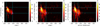 |
Fig. B.2 Same as Fig. 4, but for Monte Carlo realizations of input maps instead of masking. |
| In the text | |
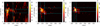 |
Fig. C.1 Same as Fig. 4, but masking regions where AV > 1.0. |
| In the text | |
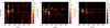 |
Fig. C.2 Same as Fig. 4, but masking regions where AV > 3.0. |
| In the text | |
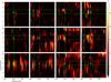 |
Fig. D.1 Same as Fig. 7, but for H I. |
| In the text | |
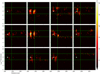 |
Fig. D.2 Same as Fig. 7, but for 13CO. |
| In the text | |
|
Fig. E.1 Correlation between the dust extinction across distances (Green et al. 2019) and H I emission across distances and velocity channels as quantified by the projected Rayleigh statistic (V) and the Pearson correlation coefficient (rPearson). |
| In the text | |
Current usage metrics show cumulative count of Article Views (full-text article views including HTML views, PDF and ePub downloads, according to the available data) and Abstracts Views on Vision4Press platform.
Data correspond to usage on the plateform after 2015. The current usage metrics is available 48-96 hours after online publication and is updated daily on week days.
Initial download of the metrics may take a while.