| Issue |
A&A
Volume 673, May 2023
|
|
|---|---|---|
| Article Number | A11 | |
| Number of page(s) | 12 | |
| Section | The Sun and the Heliosphere | |
| DOI | https://doi.org/10.1051/0004-6361/202345933 | |
| Published online | 24 April 2023 | |
Ultra-high-resolution observations of plasmoid-mediated magnetic reconnection in the deep solar atmosphere⋆
1
Institute of Theoretical Astrophysics, University of Oslo, PO Box 1029 Blindern, 0315 Oslo, Norway
e-mail: This email address is being protected from spambots. You need JavaScript enabled to view it.
2
Rosseland Centre for Solar Physics, University of Oslo, PO Box 1029 Blindern, 0315 Oslo, Norway
3
Max-Planck-Institut für Sonnensystemforschung, Justus-von-Liebig-Weg 3, 37077 Göttingen, Germany
4
Institute for Solar Physics, Dept. of Astronomy, Stockholm University, AlbaNova University Centre, 10691 Stockholm, Sweden
Received:
18
January
2023
Accepted:
22
February
2023
Abstract
Context. Magnetic reconnection in the deep solar atmosphere can give rise to enhanced emission in the Balmer hydrogen lines, a phenomenon referred to as Ellerman bombs.
Aims. To effectively trace magnetic reconnection below the canopy of chromospheric fibrils, we analyzed unique spectroscopic observations of Ellerman bombs in the Hα line.
Methods. We analyzed a 10 min data set of a young emerging active region observed with the prototype of the Microlensed Hyperspectral Imager (MiHI) at the Swedish 1-m Solar Telescope (SST). The MiHI instrument is an integral field spectrograph that is capable of achieving simultaneous ultra-high resolution in the spatial, temporal, and spectral domains. With the combination of the SST adaptive optics system and image restoration techniques, MiHI can deliver diffraction-limited observations if the atmospheric seeing conditions allow. The data set samples the Hα line over 4.5 Å with 10 mÅ pix−1, with 0.″065 pix−1 over a field of view of 8.″6 × 7.″7, and at a temporal cadence of 1.33 s. This constitutes a hyperspectral data cube that measures 132 × 118 spatial pixels, 456 spectral pixels, and 455 time steps.
Results. There were multiple sites with Ellerman bomb activity associated with strong magnetic flux emergence. The Ellerman bomb activity is very dynamic, showing rapid variability and a small-scale substructure. We found a number of plasmoid-like blobs with full-width-half-maximum sizes between 0.″1 and 0.″4 and moving with apparent velocities between 14 and 77 km s−1. Some of these blobs have Ellerman bomb spectral profiles with a single peak at a Doppler offset between 47 and 57 km s−1.
Conclusions. Our observations support the idea that fast magnetic reconnection in Ellerman bombs is mediated by the formation of plasmoids. These MiHI observations demonstrate that a microlens-based integral field spectrograph is capable of probing fundamental physical processes in the solar atmosphere.
Key words: Sun: activity / Sun: atmosphere / Sun: magnetic fields / magnetic reconnection
Movies associated to Figs. 2–6 and A.1 are available at https://www.aanda.org
© The Authors 2023
 Open Access article, published by EDP Sciences, under the terms of the Creative Commons Attribution License (https://creativecommons.org/licenses/by/4.0), which permits unrestricted use, distribution, and reproduction in any medium, provided the original work is properly cited.
This article is published in open access under the Subscribe to Open model. This email address is being protected from spambots. You need JavaScript enabled to view it. to support open access publication.
1. Introduction
Magnetic reconnection is a process that changes magnetic topologies and releases magnetic energy. It is a physical process that is fundamental for a whole range of dynamical phenomena in magnetized plasmas in environments ranging from laboratories on Earth to the heliosphere and astrophysical bodies. In the Sun, magnetic reconnection drives, for example, solar flares and coronal mass ejections and is invoked in theories that address the heating of the outer atmosphere (see, e.g., Priest 2014). In the deeper parts of the solar atmosphere, magnetic reconnection occurs in UV bursts (Young et al. 2018) and Ellerman bombs (EBs; Rutten et al. 2013). In photospheric sites where opposite magnetic polarities are in close proximity, EBs can form and exhibit remarkable enhancements of the spectral wings of the Hα line (Ellerman 1917); they appear as subarcsecond-sized brightenings with a fine structure and rapid variability in Hα wing images (see, e.g. Georgoulis et al. 2002; Pariat et al. 2007; Watanabe et al. 2008, 2011; Vissers et al. 2013; Nelson et al. 2015; Rouppe van der Voort et al. 2016).
While the macroscopic effects of magnetic reconnection are often clearly detectable in the form of, for example, morphological and structural changes, or in the form of (fast) outflows, details of the microscopic physics remain mostly elusive. Of particular interest regarding the mode of reconnection is the formation of plasmoids: small-scale magnetic structures that form when reconnection current sheets break up under the tearing instability into smaller pieces (Furth et al. 1963; Biskamp 1986). This process allows reconnection to happen faster and may explain the observed timescales of reconnection events in the solar atmosphere, which are shorter than classical reconnection theory predicts (Bhattacharjee et al. 2009; Ni et al. 2015). Plasmoid formation is in principle a small-scale process that occurs at spatial scales that are beyond the reach of present-day instrumentation. However, there have been a number of reports that provide evidence for plasmoids in the solar atmosphere. They are often observations of moving bright blobs at spatial scales near the resolution limit of imaging instruments. For example, plasmoid-like blobs have been reported in observations of coronal mass ejections (Lin et al. 2005; Gou et al. 2019), flares (Nishizuka et al. 2010; Takasao et al. 2012; Yan et al. 2022), jets (Singh et al. 2012), and rapidly evolving coronal loops (Antolin et al. 2021). Additional evidence for plasmoid formation is based on the evolution and shape of transition-region spectral lines associated with UV bursts (Innes et al. 2015; Guo et al. 2020).
The smallest reported plasmoid-like blobs have sizes below 150 km and were observed near EBs associated with UV bursts (Rouppe van der Voort et al. 2017). These EBs occurred in connection with episodes of strong magnetic flux emergence in an active region. The observed blobs and spectral line profiles were found to be in agreement with numerical simulations of flux emergence where the emerging magnetic field reconnects with the overlying canopy fields. A number of recent numerical simulations have shown that plasmoids are formed in reconnection events that produce EBs and UV bursts (Hansteen et al. 2019; Peter et al. 2019; Ni et al. 2021; Nóbrega-Siverio & Moreno-Insertis 2022).
Ellerman bombs offer a unique window on reconnection in the solar atmosphere: spectral lines in the optical can be employed to resolve the smallest possible scales and get the best possible view of the details of the reconnection process. This has been recognized as one of the prime science cases (Rast et al. 2021; Schlichenmaier et al. 2019) for the new DKIST (Rimmele et al. 2020) and EST (Quintero Noda et al. 2022) 4 m class solar telescopes. This highly dynamical process poses a formidable observational challenge: structures evolve on a timescale of a few seconds or less and move with velocities of few tens of km s−1 or more. Typical tunable filtergram instruments that have sufficient spatial and temporal resolution have limited spectral resolution and cannot cover the required spectral range within the dynamical timescale. Typical slit spectrographs that have the required resolution and spectral coverage cannot follow fast moving structures over an extended area. Integral field spectrographs can alleviate these problems. We analyzed observations from a prototype of the Microlensed Hyperspectral Imager (MiHI; van Noort et al. 2022), a microlens-based integral field spectrograph that is capable of acquiring spatially, spectrally, and temporally resolved data over an extended field of view (FOV). The data set samples the Hα line over a Doppler range of about ±100 km s−1 with 0.5 km s−1 pix−1, over a FOV of about 8.6″ × 7.7″ with  pix−1, during a period of 10 min at a temporal cadence of 1.33 s. This unique data set provides an unprecedented view of the complex dynamics of EBs in an active region with vigorous magnetic flux emergence.
2. Observations
2.1. The MiHI prototype
The observations were acquired with the Swedish 1-m Solar Telescope (SST; Scharmer et al. 2003a), where the MiHI prototype was installed as a plug-in for the TRIPPEL spectrograph (Kiselman et al. 2011). The MiHI prototype and the methods used to calibrate it and convert the raw data frames into three-dimensional form are described in some detail in a series of three publications: van Noort et al. (2022), which covers its motivation and design, van Noort & Chanumolu (2022), which outlines the modeling and characterization, and van Noort & Doerr (2022), which details the data reduction and image restoration. For convenience, we refer to the prototype simply as “MiHI” in the remainder of this paper.
MiHI has a double-sided microlens array that samples the image plane and de-magnifies each sample such that a two-dimensional array of point-like sources is passed through the spectrograph. Each bright source is then dispersed, generating a spectrum that is separated sufficiently from the spectra of neighboring sources to avoid significant spatial overlap. Spectral overlap between neighboring spectra is avoided by placing a prefilter in the beam in front of the microlens array, which limits the wavelength range.
The design of MiHI was optimized for spectropolarimetry in the Fe I line pair at 6302 Å with a spectral resolution of R = 315 000. During the 2018 observing campaign, however, spectropolarimetry was also performed in the nearby Na D1 and Hα lines (see van Noort & Doerr 2022). In this paper we concentrate on the Hα Stokes I data that were recorded on 24 August 2018.
Whenever the seeing conditions allow, the combination of two key factors, the SST adaptive optics system (Scharmer et al. 2003b, 2019) and image restoration, is able to deliver near-diffraction-limited spatial resolution in the MiHI data. The method used for the image restoration is briefly described in van Noort & Doerr (2022) and is based on an image restoration technique developed for slit spectrograph data (van Noort 2017), which restores the image information by considering that the observed data are the sum of numerous contributions from un-degraded object pixels, which are smeared out spatially according to a known point spread function (PSF). The resulting linear system connecting the data to the un-degraded object pixels was solved using a technique akin to Lucy-Richardson deconvolution. The PSF, required to be known for this technique to work, was determined from the high-cadence phase-diversity images from the context imager using the multi-frame blind deconvolution (MFBD; Löfdahl & Scharmer 1994; van Noort et al. 2005) wavefront sensing technique. The context imager was pointed at the MiHI entrance window, which consists of a 2 × 2 mm transparent area of an otherwise black-chromium-coated plano-concave lens. The reflectivities of the transparent entrance window and the surrounding coated area were designed to be comparable so that the context imager receives a comparable amount of the signal from both the MiHI FOV and its surroundings. Through the reflection off the MiHI entrance window, the context imager is capable of effectively determining the wavefront over the full MiHI FOV, a prerequisite for the restoration of the spectral data. The context imager consisted of two cameras, set up as a phase diversity pair, and operated at a frame rate of 600 Hz and with a 1.5 ms exposure time. This was considerably faster than the MiHI camera, which operated at 30 Hz and with a 30 ms exposure time. The PSF used to deconvolve the MiHI data was obtained by averaging over the PSFs of the multiple context exposures with temporal overlap with the longer MiHI exposure, thus satisfying the frozen-seeing condition that is implicitly assumed by the MFBD wavefront sensing method. In this way it is possible to accurately describe the PSF for the 30 ms exposure window of the spectral cameras, while simultaneously maximizing the amount of signal available for the wavefront sensing. The context imager acquired 20 exposures during each MiHI exposure.
Since MiHI, unlike a slit spectrograph, does not need to scan an extended region, the data can be restored with an arbitrary cadence, in principle up to the frame rate of the camera. The cadence can thus be chosen based on the expected rapid time evolution of the solar atmosphere at the heights sampled by the Hα line; it was selected to be 1.33 s (covered by 40 MiHI exposures, 10 per liquid crystal state). At such a high cadence, another implicit assumption of the MFBD wavefront sensing method, that the tip and tilt components of the wavefronts vanish when averaged over the period over which the wavefront samples were collected, is no longer satisfied accurately. As a result, the frame of reference of the restored images is still subject to significant residual differential seeing, which manifests itself as a time-dependent warping of the image.
The most obvious way to avoid this problem is to extend the time period over which the context images are collected and restore the time series at a lower cadence. The spectral data can then be restored using subsets of wavefronts, at the selected cadence of 1.33 s. Unfortunately, the filter used for the context image of MiHI is the same as that used for the spectral camera and covers only the core and inner wings of Hα. Consequently, the image is a relatively even blend of structures from a large range of heights in the solar atmosphere. This is close to ideal from the perspective of providing context for the small instrumental FOV because it contains an imprint of most structures that are visible in the spectra. From the perspective of image restoration, however, this blend of structures is less than ideal, since their mixing reduces the image contrast, which in turn reduces the reliability of the wavefront sensing. More importantly, however, due to their height in the solar atmosphere, many of these structures evolve on the same short timescale as that expected for the spectra, and restoring these data at a lower cadence does not result in a reliable estimate of the wavefronts.
To remedy this problem, the technique used by van Noort (2017) to compensate for the scanning motion of the slit in their restoration of scanning slit spectra was employed here as well. To this end, the context data for the entire time series were first reduced at the desired high cadence, but also with a significant overlap in time, so that the wavefront coefficients for the same patch of the same frame were determined in the context of different temporal acquisition windows. Since on logical grounds the tip and tilt coefficients of the same patch from the same frame must clearly always have the same value, the difference between the recovered values from two different restorations covering different time periods must be proportional to the displacement between their respective frames of reference. Since many frames were used for each restoration, many such differences can be obtained, the average value of which yields an accurate estimate for the displacements between the patches for each pair of temporally overlapping restorations.
Integration of these displacements over time yields an accurate estimate of the position of each restored patch, relative to the average position of that patch over the whole time series. This position is subsequently added to each PSF prior to executing the spectral restoration, resulting in a common frame of reference for all restored frames within the time series. With data obtained under good and stable seeing conditions, as was the case for the time series presented in this paper, results of very high stability can be obtained in this way, which need no additional compensation for residual image motion induced by atmospheric seeing or telescope rotation.
An added benefit of using the spectral restoration method is that it can make use of the PSF information to also recover information about object pixels that are located outside the instrumental FOV, giving it the ability to observe “outside the box”. This ability is a function of the width and variability of the atmospheric PSF in the specific temporal window of the restoration, but it is usually possible to extend the FOV of the instrument by approximately 2 pixels in all directions, depending somewhat on the required S/N of the restored data. With the 128 × 114 microlens array elements that were fully sampled by the spectral camera for the present time series, a restored FOV of 132 × 118 px2 could be obtained.
After restoration, the time series comprises 455 time steps, each represented by a hyperspectral cube of 132 × 118 × 456 spectral pixels (spaxels). With a spatial sampling of  px−1 and a spectral sampling of 10 mÅ px−1, this corresponds to a FOV of
  ×
×  × 4.5 Å. The wavelength range runs from 6560.5546 to 6565.0545 Å, corresponding to a Doppler offset range of about ±102 km s−1 around the nominal Hα line center and a Doppler sampling of 0.45 km s−1 px−1. There are a few weak spectral line blends in this spectral range. Most have been identified as telluric H2O lines (Moore et al. 1966) at about −78, +32, +57, and +64 km s−1. Further, there is a weak Si I line at −103 km s−1, with an effective Landé factor of approximately 1, and a very weak Co I line at +28 km s−1.
The temporal duration was 10 min and 6 s, starting at 08:03:44 UT on 24 August 2018, with a temporal cadence of 1.33 s. The seeing quality was measured by the SST adaptive optics wavefront sensor (see Scharmer et al. 2019). The Fried’s parameter, r0, for the ground-layer seeing varied between 9 and 34 cm, with the average for the first 6 min above 20 cm. The r0 for a combination of ground- and high-altitude seeing varied between 7 and 10 cm. The pointing was centered on heliocentric coordinates (x, y) = (255″, 5″), observing angle θ = 16°, and μ = cos θ = 0.96, targeting the emerging active region AR12720. We made much use of CRISPEX (Vissers & Rouppe van der Voort 2012), a graphical user interface for effective exploration of multi-dimensional data sets that is available in SolarSoft.
The spatial sampling of the context imager was  px−1, and the FOV
  ×
×  . A duplicate of the MiHI prefilter was used as a filter for the context imager. This filter has a bandwidth of about 4 Å and is centered on the Hα line so that the context images show a complex mix of both photospheric and chromospheric structures. The context images were put together in a time series with 915 time steps, at a cadence that is twice as fast as the MiHI spectral data (0.67 s). Figure 1 shows the observed FOV in the context of observations from the Solar Dynamics Observatory (SDO) and the Interface Region Imaging Spectrograph (IRIS). Figure 2 shows examples of MiHI spectral images in relation to the context image.
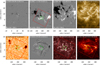 |
Fig. 1. Extended context for the MiHI observations of 24 August 2018. Panels a–c show the emergence of AR12720 in HMI BLOS magnetic field maps over a period of 48 h. Panel b has the approximate locations of the FOVs of MiHI marked in green and of the context imager in red. Panel d shows an IRIS raster map at the nominal wavelength of Mg II k observed 24 h after the MiHI observations. In the bottom row, the MiHI Hα wideband context image in panel f is accompanied by the closest available SDO images: HMI continuum (e), AIA 1700 Å (g), and AIA 304 Å (h). |
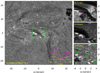 |
Fig. 2. Overview of the MiHI observations of AR12720 on 24 August 2018. The left panel shows an image from the Hα wideband context imager; the green box outlines the MiHI FOV. The column to the right shows MiHI images in the Hα core and two positions in the blue wing. Notable features are marked in the bottom-right panel: micro-pores (P1, P2, and P3), clusters with EBs (EB1 – 5), and elongated granules characteristic of strong flux emergence (G1 and G2). The pink cross marks the location in EB1 of the spectral profile shown in pink in the lower-right corner of the large context image. The yellow profile is a reference spectrum averaged over the full MiHI FOV. An animation of this figure is available online. |
2.2. Reference observations
To put the MiHI observations into an extended context, we studied observations from SDO (Pesnell et al. 2012), from both the AIA (Lemen et al. 2012) and HMI (Scherrer et al. 2012) instruments. Unfortunately, there were no strictly co-temporal SDO observations since the operations were affected due to an Earth eclipse. The earliest available SDO observations of sufficient quality were taken about 20 min after the end of the MiHI observations (see Figs. 1b,e,g,h). We made extensive use of the JHelioviewer (Müller et al. 2017) tool to explore the SDO data.
We also used IRIS (De Pontieu et al. 2014) observations of the active region taken the day after the MiHI observations. Figure 1d shows a Mg II k spectroheliogram constructed from a very large dense 320-step raster (observation identifier 20180825_064806_3620108077). This IRIS observation was taken with all four science slit-jaw channels: SJI 1330, 1400, 2796, and 2832 Å.
We further used a different SST data set that contains a similar episode of strong flux emergence with anomalously elongated granules as we find in the MiHI observations. This episode of flux emergence and associated EBs was part of a 29 min time series of AR12770 observed with the CRISP (Scharmer et al. 2008) and CHROMIS (Scharmer 2017) instruments on 11 August 2020. From CRISP we used maps of the magnetic field strength along the line of sight (BLOS) derived from Milne-Eddington inversions of the Fe I 6173 Å line. We used the inversion code developed by de la Cruz Rodríguez (2019). From CHROMIS we used observations in the Hβ line, which was sampled at 27 line positions between ±2.1 Å, and the associated wideband data (filter width 6.5 Å, centered at 4846 Å). The temporal cadence of the Hβ data was 17 s. The data were processed using the SSTRED reduction pipeline (de la Cruz Rodríguez et al. 2015; Löfdahl et al. 2021). The active region was located at (x, y) = (321″, 296″) and observed under an observing angle of θ = 27° (μ = 0.89).
3. Results
3.1. Magnetic flux emergence in AR12720
The MiHI instrument was targeting the central area of a young emerging active region that was in a state of massive flux emergence. As shown in the HMI BLOS map in Fig. 1a, 24 h earlier, the active region had only just started to emerge to the surface, while 24 h later (Fig. 1c), the active region had grown so much that it had received its NOAA active region number: AR12720. The emergence of the active region over this period was accompanied with enhanced activity in all the AIA channels, for example as bursts of compact brightenings in the AIA 1600 and 1700 Å channels. The AIA 1700 Å image in Fig. 1g shows one such brightening inside and one just outside the area that was covered by MiHI about 25 min earlier. These compact UV continuum brightenings are associated with EBs (Vissers et al. 2019b).
The AIA 304 Å channel, dominated by the He II resonance line, showed high levels of enhanced emission in and around the emerging region, as well as long dark fibrils that obscure some of the emission from the deeper parts of the atmosphere. Some of these dark fibrils are visible in Fig. 1h. Long dark chromospheric fibrils are clearly visible in the IRIS Mg II k raster map in Fig. 1d. These fibrils form a chromospheric canopy of preexisting magnetic fields that the newly emerging magnetic flux encounters from below as it rises through the lower atmosphere. These encounters lead to the magnetic reconnection and dissipation of currents, which is associated with impulsive heating and flaring loops, as can be seen, for example, in the IRIS transition-region slit-jaw channels SJI 1330 and 1400 Å.
The densest chromospheric fibrils were also visible in the MiHI context images (Fig. 1f and large panel in Fig. 2). These fibrils had sufficient opacity over the filter passband to effectively block radiation from the deeper atmosphere below.
From the context SDO and IRIS observations, we conclude that MiHI was targeting the heart of a region in the middle of an extended period of strong magnetic flux emergence. Earlier emerged flux had already established an overlying chromospheric canopy of dense fibrils. New magnetic flux that freshly appeared at the surface just prior to or during the short, 10 min, duration of the MiHI observation was caught in the process of interacting with the preexisting ambient magnetic field. While there are no detailed measurements of the magnetic field and the magnetic field topology is therefore unknown, such a region with strong flux emergence is known to have a high occurrence of EBs (see, e.g., Georgoulis et al. 2002).
3.2. Ellerman bombs
Figure 2 shows example MiHI images at three different spectral positions and the associated wideband context image. The wideband channel integrates over the full Hα prefilter passband and shows a mix of both chromospheric and photospheric structures. A large system of chromospheric fibrils was crossing the MiHI FOV; the accompanying animation shows that they consist of long and narrow threads. Some chromospheric structures have strong Doppler shifts and are visible in the Hα wing images. The far blue wing MiHI image shows the clearest view at the underlying photosphere. Here we can identify three micro-pores, marked as P1, P2, and P3. Micro-pore P1, in the lower-left corner, is the largest; P2 and P3 are smaller and less dark in their central areas. All micro-pores are surrounded by bright rims with bright points and have a similar morphology as the small micro-pores and ribbons that were described by Berger et al. (2004) and Rouppe van der Voort et al. (2005).
Throughout the 10 min duration of the observation, there are a number of EBs at different locations in the FOV. In the far blue wing MiHI image of Fig. 2, five different sites with clusters of EBs are marked as EB1 – 5. Cluster EB5 is not very bright in Fig. 2, but it can be seen with clear enhanced brightness earlier and later in the accompanying movie. The three MiHI panels are a nice illustration that EBs reside below the chromosphere: there are no clear EB signatures in the line core image, while the far wing image shows an unobstructed view of the EB sites (this was earlier shown by Watanabe et al. 2011). In the intermediate wing position (middle panel), EBs are partly covered by overlying chromospheric structures. This is best seen in the movie.
Example EB profiles from three different EB clusters are shown in Fig. 3. They show the characteristic EB profile with a central absorption core, a peak intensity in the wings at around a ±1 Å offset from line center, and a decreasing intensity towards larger wavelength offsets. These are very strong EBs: the peak intensity reaches up to three or more times the reference intensity from the average profile. This is more than double the typical threshold value that is used for automatic EB detection methods (see Vissers et al. 2019b). The enhanced wing emission extends over a wide wavelength range, probably far beyond the ±2.2 Å wavelength range of the MiHI observations, as one can infer from a naive visual extrapolation of the far wing profile trends. The animation of the spectral line scan that accompanies Fig. 3 is another vivid illustration that EBs are situated below the chromosphere as they become increasingly covered by chromospheric structures for smaller offsets from line center. The other animation accompanying Fig. 3 shows the temporal evolution at a −70 km s−1 Doppler offset and detailed spectral evolution for a location in the EB1 cluster. The movie clearly shows the bursty character and rapid evolution of this EB cluster. A large number of small and faint blobs can be seen to be ejected. These blobs will be discussed in more detail further below.
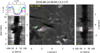 |
Fig. 3. Example EB profiles. The middle panel shows a MiHI Hα blue wing image. Colored crosses mark the locations of the spectral profiles shown in the top-left panel. Profiles are shown from EB clusters (see Fig. 1) EB1 (pink), EB2 (green), and EB4 (blue). The gray profile is averaged over the whole FOV and serves as a reference. All profiles are normalized to the far blue wing intensity of the reference profile. The lower-left panel shows the spectral evolution for the location marked with the pink cross as a λt diagram. The right panel shows the spectra along the dotted yellow line in the Hα wing image as a λy diagram. Horizontal dotted pink lines in the two diagrams mark the pink profile. Small vertical yellow markers indicate the spectral position of the Hα wing image. Two animations of this figure are available online, one showing the full temporal evolution and one showing a spectral line scan stepping through the full spectral range. |
3.3. Anomalously elongated granules
The EBs in the EB1 and EB2 clusters are at the ends of what appear to be abnormally long and elongated granules, marked as G1 and G2 in the far wing panel of Fig. 2. The evolution of these elongated granules is shown in the summed Hα far wing images in Fig. 4 and the associated animation. Anomalously elongated granules can be regarded as a characteristic sign of the emergence of strong magnetic flux (Cheung et al. 2008; Guglielmino et al. 2010; Ortiz et al. 2014; Cheung & Isobe 2014). The small and crowded FOV of MiHI and the relatively low granulation contrast of the Hα prefilter make it difficult to recognize the elongated granules. As a reference, Fig. 5 shows CRISP BLOS magnetograms and CHROMIS observations of a similar episode of strong magnetic flux emergence in an active region. The accompanying movie shows the emergence of magnetic flux with two opposite polarity patches moving apart. These two opposite polarity patches reside at the end points of an anomalously elongated granule. The WB 4846 Å image in Fig. 5 shows that this granule is divided in the middle along its major axis by a darker lane. Cheung & Isobe (2014) remarked that flux emergence simulations show that such dark lanes are coincident with upflows. The Hβ wing image shows clear EBs when the negative polarity patch collides with the preexisting positive polarity patches. These EBs show similar rapid and bursty evolution as in the MiHI data but at a much slower temporal sampling (17 s). Some of the time steps show the ejection of small faint blobs.
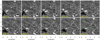 |
Fig. 4. Evolution of anomalously elongated granules in a series of MiHI Hα far wing images. The images are summed over ten spectral positions in both the blue and red wings. The labels G1 and G2 in the lower-right panel mark the two prominent elongated granules (also see Fig. 2). An animation of this figure is available online. |
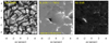 |
Fig. 5. Episode of strong flux emergence with characteristic elongated granules in 11 August 2020 CHROMIS and CRISP observations. The left panel shows a wideband (FWHM 6.5 Å) image centered on 4846 Å. The middle panel shows a map of the magnetic field BLOS derived from inversions of the Fe I 6173 Å line. The right panel shows an Hβ blue wing image at the wavelength offset of the peak of the typical EB profile. This image is scaled linearly between the minimum and maximum. An animation of this figure is available online. |
3.4. Plasmoid-like blobs
Figure 6 shows light curves from locations where bright blobs can be seen crossing. These locations are at quite a distance from the EB cluster from which the blobs appear to be originating. For the light curve in the upper left (marked L1), at time t = 5.53 min, an elongated blob can be seen to pass under the location marked with the pink cross in the Hα wing image. Its full-width-half-maximum (FWHM) size along the longest dimension is  and along the shortest dimension
  . As can be seen in the accompanying movie, it appears to be connected to the EB1 cluster, which has its root at a distance of about 2″. For a period of about 17 s, the light curve at a −73 km s−1 Doppler offset shows a clear enhancement, peaking at about 1.5 times the reference intensity. The spectral profile (shown as the pink profile in the λt diagram) shows a clear EB-like wing enhancement.
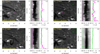 |
Fig. 6. Examples of rapid temporal variability in light curves close to EB clusters. The top row shows two examples in the vicinity of cluster EB1, and the bottom-left panel shows an example close to EB4. In the Hα wing images (left column), a pink cross marks the location of the λt diagram and the light curve (pink) in the right column. The Hα wing image is shown for a time when a blob can be seen at this location. Line profiles from this time are overplotted on the λt diagram. The light curve is at the wavelength marked with a vertical pink line in the λt diagram and noted in the top left of the MiHI wing image. The wavelength is selected to avoid excursions of the Hα line core as much as possible so that the light curve variations can be mostly attributed to EB variability. The green light curve serves as a reference and is drawn from the location marked with the green cross. The light curves are normalized by a reference light curve that is constructed by spatial averaging over the rectangular area in the top-right corner of the FOV that is marked in dark green in the bottom right. This spatially averaged spatial light curve is shown in dark green in the bottom-right light curve panel (L4) and is normalized to its temporally averaged value. A background gray line serves as a guide to I/Iref = 1.0. Animations of the figures for L1, L2, and L3 are available online. |
The light curve in the upper right (L2) is from a location closer to EB1 and shows more bursty behavior with short episodes of enhancements than L1. The accompanying movie shows that these enhancements come from many small blobs passing under the pink cross. At t = 0.33 min, the blob that is crossing has FWHM sizes  by
by  . The line profile shows a peak EB wing enhancement of more than a factor of 2.
The light curve L3 close to EB4 near the edge of the FOV shows bursty intensity peaks only in the first 2 min. The blob that passed at t = 0.51 min was round with a FWHM of  and made the Hα −57 km s−1 light curve peak for about 12 s. The blob has an EB-like spectral profile with peak intensity larger than 1.5. The EB activity in the EB4 cluster continued for a few more minutes, and the light curve remained slightly enhanced until about t = 5 min. For the last 3 min, all EB activity is gone and the light curve is very similar to the quiet reference light curve. The L4 light curve shows the reference light curve that is shown in the other panels in comparison with a light curve averaged over an area of
  .
.
Two additional light curves are shown in Fig. A.1. Light curve L5 is close to EB1, and bright blobs pass for about 50 s. At t = 1.02 min, the shortest FWHM of the passing blob is  , and the longest is
  . Light curve L6 is close to EB5 near the edge of the FOV.
The blobs are small, faint, and dynamic. We managed to make an estimate of the apparent speed for a few blobs by tracing their trajectories and constructing space-time diagrams. In Fig. 7 the curved trajectory of an elongated blob ( by
by  ) is shown in the large Hα wing image. The st diagram in the lower right shows the motion of the blobs as a bright inclined streak. The inclination of this streak is equivalent to an apparent speed of about 55 km s−1. The st diagram shows more inclined streaks caused by other blobs passing the trajectory at other times. Their inclination is similar, but it should be noted that this particular trajectory may not optimally trace the path of blobs other than the one centered at t = 0. The column of small Hα wing images shows the position of the blob at three instances of time. The blob’s spectral profiles are shown in the profile panel. The profiles are EB-like and have peak wing enhancement at about 1.7 times the reference intensity.
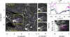 |
Fig. 7. Apparent motion of plasmoid-like blobs. The pink line in the large Hα wing image to the left traces the trajectory of some bright blobs. The st diagram for this trajectory is shown in the bottom right. The column of smaller images shows three different time steps; colored crosses mark the moving blob for which the respective spectral profiles are shown in the top-right panel. This blob has an apparent speed of about 55 km s−1, a speed that is indicated by a straight pink line in the st diagram. The pink profile in the top-right panel is a reference EB profile that is marked with the large pink cross in the large image to the left. The cross is near the origin of the trajectory for the st diagram. The gray profile is a reference profile that was constructed by averaging over the full FOV. |
The blob that is traced in Fig. 8 is associated with EB4 and is moving at an apparent speed of about 17 km s−1. The profiles of this blob have a stronger peak intensity than the blob in Fig. 7, with a maximum well above 2. These two blobs appear to be moving away from their respective EB sites. The blob traced in Fig. 9 is associated with EB3 and appears to be moving towards the EB site with an apparent speed of 14 km s−1. The profiles of this blob are very strong EB profiles. The st diagram in Fig. A.2 traces very fast blobs that appear to move at a speed of about 77 km s−1.
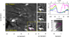 |
Fig. 8. Another example of the apparent motion of plasmoid-like blobs. The format is the same as in Fig. 7. |
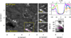 |
Fig. 9. Another example of the apparent motion of plasmoid-like blobs. The format is the same as in Fig. 7. |
Ellerman bombs occur in the deep atmosphere below the chromospheric canopy, and it seems unlikely that one can observe a complete Hα profile from the EB site itself, which is not affected by opacity from unrelated plasma in the overlying chromospheric fibrils. A “naked” EB profile from a site without an overlying chromosphere would presumably have a single emission peak without the strong central absorption around the nominal Hα line center that effectively produces the characteristic pair of peaks in the canonical EB profile. Flares can produce pure emission lines in Hα, and the peak wavelength position is a rather straightforward Doppler diagnostic in flare ribbons. The positions of the EB peaks in profiles, as in the examples shown in Fig. 3, are meaningless as a Doppler diagnostic and are clearly affected by the Doppler shift and width of the overlying chromospheric structures. However, for a few blobs, we find highly asymmetric profiles with a single emission peak in one of the wings and a seemingly unaffected wing shape at the opposite side of the line core.
Figure 10 shows four examples. The top-left example has a spectral profile with an emission peak with I/Iref > 1.7 at a Doppler offset of about −56 km s−1. The red wing does not show significantly enhanced emission. The Hα line core absorption seems to be blueshifted with the line minimum at about −20 km s−1. The line core absorption profile is slightly wider than the rather quiet profiles near the bottom of the λy diagram below y = −3″, but the red wing of the blob profile is certainly not as affected by absorption as the wide Hα profiles for  to
to  . The red wing profiles in this part of the λy diagram are totally dominated by the downflow of a surge-like event. The spectral profile for this example seems to not have a red wing EB peak, and it is therefore suggestive that the EB emission comes from strongly blueshifted plasma. The −56 km s−1 offset of the peak intensity is probably an upper limit since it seems likely that the position of the emission peak is affected by the blueshifted Hα absorption core.
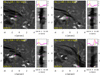 |
Fig. 10. Four examples of highly asymmetric spectral profiles that are suggestive of Doppler-shifted emission peaks. The pink cross in the Hα wing images (to the left) marks the location of the full spectral profile shown in the top right (pink profile). The gray profile is a reference profile averaged over the full MiHI FOV. The spectral profiles are normalized to the intensity at the shortest wavelength of the reference profile. The vertical dashed yellow line marks the location of the λy diagram shown to the right. |
The upper-right example is from a different time in the same region and shows peak intensity at about −52 km s−1. The line core absorption has a similar width as the reference profile and does not appear to be Doppler-shifted. The red wing shows no sign of EB emission and closely follows the reference profile. The red wing of the lower-left example is also not affected, and this profile has a rather weak line core absorption that has a higher intensity than the reference profile. The peak intensity is at about −57 km s−1.
The fourth example, in the lower right, is from a different region and is associated with the EB3 site, where blobs can be seen moving towards the EB root site (see Fig. 9). The spectral profile shows a very strong emission peak of nearly 3 at a Doppler offset of +47 km s−1. There is very strong Hα line core absorption that is blueshifted, with the line minimum at about −30 km s−1. This can be attributed to a chromospheric upflow above the blob and affects the inner wing only. The far blue wing, however, does not show any enhanced emission. The redshift of this emission peak is suggestive of a downflow, which is consistent with the apparent inflow that can be seen in this region. The blueshifts of the emission peaks of the other three examples indicate outflows that are consistent with the apparent motion of blobs away from the EB1 site.
4. Discussion and conclusion
We analyzed ultra-high-resolution Hα observations from a prototype of the MiHI microlens-based integral field spectrograph targeting the heart of a young emerging active region. The data set combines unprecedented simultaneous high resolution in three domains: spatial resolution better than  , spectral resolution of R ≈ 315 000 (about 20 mÅ at 6563 Å), and a temporal cadence of 1.33 s. Context SDO and IRIS observations show that there was a high level of magnetic flux emergence and activity related to interactions between newly emerged and preexisting ambient flux. At the photospheric level, the MiHI observations show the evolution of at least two anomalously elongated granules that are characteristic of strong magnetic flux emergence. A high level of EB activity was found to be associated with these elongated granules, and in total five sites with more or less continuous and strong EB activity were found over the 10 min time series and
  MiHI FOV. These EB sites were clearly situated below the chromosphere as they were mostly visible in the far Hα wings and completely covered in spectral images around the line core. The EB activity displayed high variability on a timescale of seconds, both in terms of wing intensity and in terms of spatial morphology and extent of the area covered in the FOV. The EB areas had a clear substructure, and there were multiple episodes where small blobs could be observed to detach from the EB sites and move away at high speeds. These blobs were found to have sizes below
  down to the diffraction limit; we measured FWHM sizes between
  and
and  . From st diagrams, the apparent speeds of four blobs were measured, and we found approximate speeds between 14 and 77 km s−1. The blobs had EB-like spectral profiles with peak wing enhancement often well above 1.5 times the reference wing intensity, surpassing common enhancement thresholds that are used for the automatic detection of EBs (Vissers et al. 2019b). We found a few examples where the blob spectral profiles have only one emission peak and the opposite spectral wing appears to be unaffected by overlying chromospheric absorption. For these examples, the Doppler offset of the peak intensity could serve as a velocity diagnostic of the EB-emitting plasma. The Doppler offsets range between 47 and 57 km s−1. These values should be regarded as upper limits since the peak profile and position is most likely affected by the overlying chromosphere. Still, these single peak profiles are a cleaner Doppler diagnostic than the canonical double peaked EB profiles. These Doppler velocities have values that are consistent with the apparent speeds. Moreover, we find blueshifts for blobs that appear to move away from their EB root sites and a redshift for a blob that is part of a group of blobs that is moving towards the EB site.
High temporal variability in EBs was earlier found in 1 s cadence wideband Hα observations (Watanabe et al. 2011; Rouppe van der Voort et al. 2016). Since these observations were filtergram data, they lacked the extensive spectral coverage of the MiHI data we analyzed here. The active region EBs analyzed in Watanabe et al. (2011) were found to have substructure features moving up with apparent speeds between 11 and 60 km s−1 and down with speeds between 7 and 18 km s−1. Our measurements for apparent speed and inferred Doppler velocities are consistent with these values.
Rouppe van der Voort et al. (2017) observed a fine structure and rapid variability in CHROMIS Ca II K observations of EBs associated with magnetic flux emergence. Bright blobs with FWHM sizes smaller than  were found in spectral images at Doppler offsets of about 40 km s−1. The temporal cadence was longer than 10 s, and no reliable measurements of the apparent velocity could be made. The EBs were associated with UV bursts, and the IRIS Si IV profiles that were co-spatial and co-temporal with the Ca II K blobs were of non-Gaussian and triangular shape. These types of profiles have been linked to magnetic reconnection driven by the plasmoid instability (Innes et al. 2015). Guo et al. (2020) simulated the onset of fast reconnection in a thinning current sheet that breaks up into multiple plasmoids. As the plasmoids grow and coalesce, they adopt a broad range of velocities that collectively produce wide and non-Gaussian Si IV profiles. The dynamic evolution of the simulated Si IV profiles matched well with high cadence IRIS observations of UV bursts. Rouppe van der Voort et al. (2017) compared the Ca II K and Si IV observations with synthetic observables computed from a two-dimensional Bifrost simulation of magnetic flux emergence (Nóbrega-Siverio et al. 2017). In this simulation, plasmoids occur in the current sheet that forms during the coalescence of the newly emerging field with the preexisting canopy. The favorable similarity between the synthetic and observed spectral line profiles supports the idea that the small-scale and highly dynamic blobs in the SST observations are in fact plasmoids that are produced in reconnection in the deep solar atmosphere. A similar SST observation was reported by Díaz Baso et al. (2021), who tracked a number of
  sized blobs in the blue wing of the Ca II K line being ejected from a region with strong reconnection, also associated with magnetic flux emergence. The blobs were identified at a Doppler offset of −100 km s−1, and their apparent speed in the ∼9 s cadence time sequence was estimated to range between 70 and 100 km s−1.
The similarities with these earlier high-resolution observations support the interpretation that the blobs in the Hα MiHI observations are plasmoids. A strong advantage of MiHI is that it removes the classic limitations of either tunable filtergraphs, such as CHROMIS, or scanning spectrographs, such as IRIS, and delivers simultaneous high resolution in many domains. These Hα observations illustrate that this allows the fundamental process of magnetic reconnection in the deep solar atmosphere to be better characterized. While the interpretation of the Hα line is challenging due to its complex spectral line formation, it is possible to get a clearer view of EB sites in the shorter wavelength Balmer lines (Joshi et al. 2020). Not only does the shorter wavelength allow for higher spatial resolution and higher intensity contrast, the higher order Balmer lines are also less affected by opacity in the overlying chromosphere. The CHROMIS observations of the EB in Fig. 5 show that plasmoid-like blobs can also be detected in Hβ. This is an exciting prospect that the next generation of 4 m class telescopes should be capable of zooming in on even smaller spatial scales. Among many other elementary questions, this may resolve the question of whether these  blobs really are single plasmoids or rather conglomerates of multiple, smaller plasmoids. Our observations make a strong case that a MiHI-like integral field spectrograph at a 4 m class telescope is a powerful combination, which, aided with modern non-LTE inversions (e.g., Vissers et al. 2019a) and advanced numerical simulations (e.g., Nóbrega-Siverio & Moreno-Insertis 2022), is ideally suited to make fundamental progress in the understanding of the physics of the solar atmosphere.
Movies
Movie 1 associated with Fig. 2 (rouppe_mihi_fig02) Access Supplementary Material
Movie 2 associated with Fig. 3 (rouppe_mihi_fig03_linescan) Access Supplementary Material
Movie 3 associated with Fig. 3 (rouppe_mihi_fig03_tevolution) Access Supplementary Material
Movie 4 associated with Fig. 4 (rouppe_mihi_fig04) Access Supplementary Material
Movie 5 associated with Fig. 5 (rouppe_mihi_fig05) Access Supplementary Material
Movie 6 associated with Fig. 6 (rouppe_mihi_fig06_L1) Access Supplementary Material
Movie 7 associated with Fig. 6 (rouppe_mihi_fig06_L2) Access Supplementary Material
Movie 8 associated with Fig. 6 (rouppe_mihi_fig06_L3) Access Supplementary Material
Movie 9 associated with Fig. A.1 (rouppe_mihi_figA1_L5) Access Supplementary Material
Movie 10 associated with Fig. A.1 (rouppe_mihi_figA1_L6) Access Supplementary Material
Acknowledgments
The Swedish 1-m Solar Telescope is operated on the island of La Palma by the Institute for Solar Physics of Stockholm University in the Spanish Observatorio del Roque de los Muchachos of the Instituto de Astrofísica de Canarias. The Institute for Solar Physics is supported by a grant for research infrastructures of national importance from the Swedish Research Council (registration number 2021-00169). IRIS is a NASA small explorer mission developed and operated by LMSAL with mission operations executed at NASA Ames Research center and major contributions to downlink communications funded by ESA and the Norwegian Space Centre. This research is supported by the Research Council of Norway, project numbers 250810, 325491, and through its Centres of Excellence scheme, project number 262622. This project was supported by the European Commission’s FP7 Capacities Program under the Grant Agreements Nos. 212482 and 312495. It was also supported by the European Union’s Horizon 2020 research and innovation program under the Grant Agreements Nos. 653982 and 824135. This project has received funding from the European Research Council (ERC) under the European Union’s Horizon 2020 research and innovation program: grant agreement No. 695075 (MvN) and SUNMAG, grant agreement 759548 (JdlCR). This work benefited from discussions during the workshop “Studying magnetic-field-regulated heating in the solar chromosphere” (team 399) at the International Space Science Institute (ISSI) in Switzerland. We thank Dr. D. Nóbrega Siverio for illuminating discussions. We made much use of NASA’s Astrophysics Data System Bibliographic Services.
References
- Antolin, P., Pagano, P., Testa, P., et al. 2021, Nat. Astron., 5, 54 [NASA ADS] [CrossRef] [Google Scholar]
- Berger, T. E., Rouppe van der Voort, L. H. M., Löfdahl, M. G., et al. 2004, A&A, 428, 613 [NASA ADS] [CrossRef] [EDP Sciences] [Google Scholar]
- Bhattacharjee, A., Huang, Y.-M., Yang, H., & Rogers, B. 2009, Phys. Plasmas, 16, 112102 [Google Scholar]
- Biskamp, D. 1986, Phys. Fluids, 29, 1520 [Google Scholar]
- Cheung, M. C. M., & Isobe, H. 2014, Liv. Rev. Sol. Phys., 11, 3 [Google Scholar]
- Cheung, M. C. M., Schüssler, M., Tarbell, T. D., & Title, A. M. 2008, ApJ, 687, 1373 [Google Scholar]
- de la Cruz Rodríguez, J. 2019, A&A, 631, A153 [NASA ADS] [CrossRef] [EDP Sciences] [Google Scholar]
- de la Cruz Rodríguez, J., Löfdahl, M. G., Sütterlin, P., Hillberg, T., & Rouppe van der Voort, L. 2015, A&A, 573, A40 [NASA ADS] [CrossRef] [EDP Sciences] [Google Scholar]
- De Pontieu, B., Title, A. M., Lemen, J. R., et al. 2014, Sol. Phys., 289, 2733 [Google Scholar]
- Díaz Baso, C. J., de la Cruz Rodríguez, J., & Leenaarts, J. 2021, A&A, 647, A188 [NASA ADS] [CrossRef] [EDP Sciences] [Google Scholar]
- Ellerman, F. 1917, ApJ, 46, 298 [NASA ADS] [CrossRef] [Google Scholar]
- Furth, H. P., Killeen, J., & Rosenbluth, M. N. 1963, Phys. Fluids, 6, 459 [Google Scholar]
- Georgoulis, M. K., Rust, D. M., Bernasconi, P. N., & Schmieder, B. 2002, ApJ, 575, 506 [Google Scholar]
- Gou, T., Liu, R., Kliem, B., Wang, Y., & Veronig, A. M. 2019, Sci. Adv., 5, 7004 [Google Scholar]
- Guglielmino, S. L., Bellot Rubio, L. R., Zuccarello, F., et al. 2010, ApJ, 724, 1083 [Google Scholar]
- Guo, L. J., De Pontieu, B., Huang, Y. M., Peter, H., & Bhattacharjee, A. 2020, ApJ, 901, 148 [NASA ADS] [CrossRef] [Google Scholar]
- Hansteen, V., Ortiz, A., Archontis, V., et al. 2019, A&A, 626, A33 [NASA ADS] [CrossRef] [EDP Sciences] [Google Scholar]
- Innes, D. E., Guo, L. J., Huang, Y. M., & Bhattacharjee, A. 2015, ApJ, 813, 86 [Google Scholar]
- Joshi, J., Rouppe van der Voort, L. H. M., & de la Cruz Rodríguez, J. 2020, A&A, 641, L5 [EDP Sciences] [Google Scholar]
- Kiselman, D., Pereira, T. M. D., Gustafsson, B., et al. 2011, A&A, 535, A14 [NASA ADS] [CrossRef] [EDP Sciences] [Google Scholar]
- Lemen, J. R., Title, A. M., Akin, D. J., et al. 2012, Sol. Phys., 275, 17 [Google Scholar]
- Lin, J., Ko, Y. K., Sui, L., et al. 2005, ApJ, 622, 1251 [NASA ADS] [CrossRef] [Google Scholar]
- Löfdahl, M. G., & Scharmer, G. B. 1994, A&AS, 107, 243 [NASA ADS] [Google Scholar]
- Löfdahl, M. G., Hillberg, T., de la Cruz Rodríguez, J., et al. 2021, A&A, 653, A68 [Google Scholar]
- Moore, C. E., Minnaert, M. G. J., & Houtgast, J. 1966, The Solar Spectrum 2935 A to 8770 A (Washington: US Government Printing Office (USGPO)) [Google Scholar]
- Müller, D., Nicula, B., Felix, S., et al. 2017, A&A, 606, A10 [Google Scholar]
- Nelson, C. J., Scullion, E. M., Doyle, J. G., et al. 2015, ApJ, 798, 19 [Google Scholar]
- Ni, L., Kliem, B., Lin, J., & Wu, N. 2015, ApJ, 799, 79 [Google Scholar]
- Ni, L., Chen, Y., Peter, H., Tian, H., & Lin, J. 2021, A&A, 646, A88 [NASA ADS] [CrossRef] [EDP Sciences] [Google Scholar]
- Nishizuka, N., Takasaki, H., Asai, A., & Shibata, K. 2010, ApJ, 711, 1062 [NASA ADS] [CrossRef] [Google Scholar]
- Nóbrega-Siverio, D., & Moreno-Insertis, F. 2022, ApJ, 935, L21 [CrossRef] [Google Scholar]
- Nóbrega-Siverio, D., Martínez-Sykora, J., Moreno-Insertis, F., & Rouppe van der Voort, L. 2017, ApJ, 850, 153 [CrossRef] [Google Scholar]
- Ortiz, A., Bellot Rubio, L. R., Hansteen, V. H., et al. 2014, ApJ, 781, 126 [NASA ADS] [CrossRef] [Google Scholar]
- Pariat, E., Schmieder, B., Berlicki, A., et al. 2007, A&A, 473, 279 [NASA ADS] [CrossRef] [EDP Sciences] [Google Scholar]
- Pesnell, W. D., Thompson, B. J., & Chamberlin, P. C. 2012, Sol. Phys., 275, 3 [Google Scholar]
- Peter, H., Huang, Y. M., Chitta, L. P., & Young, P. R. 2019, A&A, 628, A8 [NASA ADS] [CrossRef] [EDP Sciences] [Google Scholar]
- Priest, E. 2014, Magnetohydrodynamics of the Sun (Cambridge: Cambridge University Press) [Google Scholar]
- Quintero Noda, C., Schlichenmaier, R., Bellot Rubio, L. R., et al. 2022, A&A, 666, A21 [NASA ADS] [CrossRef] [EDP Sciences] [Google Scholar]
- Rast, M. P., Bello González, N., Bellot Rubio, L., et al. 2021, Sol. Phys., 296, 70 [NASA ADS] [CrossRef] [Google Scholar]
- Rimmele, T. R., Warner, M., Keil, S. L., et al. 2020, Sol. Phys., 295, 172 [Google Scholar]
- Rouppe van der Voort, L. H. M., Hansteen, V. H., Carlsson, M., et al. 2005, A&A, 435, 327 [NASA ADS] [CrossRef] [EDP Sciences] [Google Scholar]
- Rouppe van der Voort, L. H. M., Rutten, R. J., & Vissers, G. J. M. 2016, A&A, 592, A100 [NASA ADS] [CrossRef] [EDP Sciences] [Google Scholar]
- Rouppe van der Voort, L., De Pontieu, B., Scharmer, G. B., et al. 2017, ApJ, 851, L6 [Google Scholar]
- Rutten, R. J., Vissers, G. J. M., Rouppe van der Voort, L. H. M., Sütterlin, P., & Vitas, N. 2013, J. Phys. Conf. Ser., 440, 012007 [Google Scholar]
- Scharmer, G. 2017, SOLARNET IV: The Physics of the Sun from the Interior to the Outer Atmosphere, 85 [Google Scholar]
- Scharmer, G. B., Bjelksjö, K., Korhonen, T. K., et al. 2003a, Proc. SPIE, 4853, 341 [NASA ADS] [CrossRef] [Google Scholar]
- Scharmer, G. B., Dettori, P. M., Löfdahl, M. G., & Shand, M. 2003b, Proc. SPIE, 4853, 370 [NASA ADS] [CrossRef] [Google Scholar]
- Scharmer, G. B., Narayan, G., Hillberg, T., et al. 2008, ApJ, 689, L69 [Google Scholar]
- Scharmer, G. B., Löfdahl, M. G., Sliepen, G., & de la Cruz Rodríguez, J. 2019, A&A, 626, A55 [NASA ADS] [CrossRef] [EDP Sciences] [Google Scholar]
- Scherrer, P. H., Schou, J., Bush, R. I., et al. 2012, Sol. Phys., 275, 207 [Google Scholar]
- Schlichenmaier, R., Bellot Rubio, L. R., Collados, M., et al. 2019, ArXiv e-prints [arXiv:1912.08650] [Google Scholar]
- Singh, K. A. P., Isobe, H., Nishizuka, N., Nishida, K., & Shibata, K. 2012, ApJ, 759, 33 [NASA ADS] [CrossRef] [Google Scholar]
- Takasao, S., Asai, A., Isobe, H., & Shibata, K. 2012, ApJ, 745, L6 [Google Scholar]
- van Noort, M. 2017, A&A, 608, A76 [NASA ADS] [CrossRef] [EDP Sciences] [Google Scholar]
- van Noort, M., & Chanumolu, A. 2022, A&A, 668, A150 [NASA ADS] [CrossRef] [EDP Sciences] [Google Scholar]
- van Noort, M., & Doerr, H. P. 2022, A&A, 668, A151 [NASA ADS] [CrossRef] [EDP Sciences] [Google Scholar]
- van Noort, M., Rouppe van der Voort, L., & Löfdahl, M. G. 2005, Sol. Phys., 228, 191 [Google Scholar]
- van Noort, M., Bischoff, J., Kramer, A., Solanki, S. K., & Kiselman, D. 2022, A&A, 668, A149 [NASA ADS] [CrossRef] [EDP Sciences] [Google Scholar]
- Vissers, G., & Rouppe van der Voort, L. 2012, ApJ, 750, 22 [Google Scholar]
- Vissers, G. J. M., Rouppe van der Voort, L. H. M., & Rutten, R. J. 2013, ApJ, 774, 32 [NASA ADS] [CrossRef] [Google Scholar]
- Vissers, G. J. M., de la Cruz Rodríguez, J., Libbrecht, T., et al. 2019a, A&A, 627, A101 [NASA ADS] [CrossRef] [EDP Sciences] [Google Scholar]
- Vissers, G. J. M., Rouppe van der Voort, L. H. M., & Rutten, R. J. 2019b, A&A, 626, A4 [NASA ADS] [CrossRef] [EDP Sciences] [Google Scholar]
- Watanabe, H., Kitai, R., Okamoto, K., et al. 2008, ApJ, 684, 736 [Google Scholar]
- Watanabe, H., Vissers, G., Kitai, R., et al. 2011, ApJ, 736, 71 [NASA ADS] [CrossRef] [Google Scholar]
- Yan, X., Xue, Z., Jiang, C., et al. 2022, Nat. Commun., 13, 640 [NASA ADS] [CrossRef] [Google Scholar]
- Young, P. R., Tian, H., Peter, H., et al. 2018, Space Sci. Rev., 214, 120 [Google Scholar]
Appendix A: More examples
Two more light curves are shown in Fig. A.1, one close to EB cluster EB1 and one close to EB5. One additional example of the apparent motion of plasmoid-like blobs is shown in Fig. A.2.
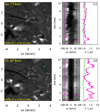 |
Fig. A.1. Two additional light curves (see Fig. 6). Light curve L5 is close to EB cluster EB1, L6 close to EB5 (see Fig. 2). Animations of this figure are available online. |
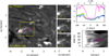 |
Fig. A.2. Another example of the apparent motion of plasmoid-like blobs. The format is the same as in Fig. 7. |
All Figures
|
Fig. 1. Extended context for the MiHI observations of 24 August 2018. Panels a–c show the emergence of AR12720 in HMI BLOS magnetic field maps over a period of 48 h. Panel b has the approximate locations of the FOVs of MiHI marked in green and of the context imager in red. Panel d shows an IRIS raster map at the nominal wavelength of Mg II k observed 24 h after the MiHI observations. In the bottom row, the MiHI Hα wideband context image in panel f is accompanied by the closest available SDO images: HMI continuum (e), AIA 1700 Å (g), and AIA 304 Å (h). |
| In the text | |
|
Fig. 2. Overview of the MiHI observations of AR12720 on 24 August 2018. The left panel shows an image from the Hα wideband context imager; the green box outlines the MiHI FOV. The column to the right shows MiHI images in the Hα core and two positions in the blue wing. Notable features are marked in the bottom-right panel: micro-pores (P1, P2, and P3), clusters with EBs (EB1 – 5), and elongated granules characteristic of strong flux emergence (G1 and G2). The pink cross marks the location in EB1 of the spectral profile shown in pink in the lower-right corner of the large context image. The yellow profile is a reference spectrum averaged over the full MiHI FOV. An animation of this figure is available online. |
| In the text | |
|
Fig. 3. Example EB profiles. The middle panel shows a MiHI Hα blue wing image. Colored crosses mark the locations of the spectral profiles shown in the top-left panel. Profiles are shown from EB clusters (see Fig. 1) EB1 (pink), EB2 (green), and EB4 (blue). The gray profile is averaged over the whole FOV and serves as a reference. All profiles are normalized to the far blue wing intensity of the reference profile. The lower-left panel shows the spectral evolution for the location marked with the pink cross as a λt diagram. The right panel shows the spectra along the dotted yellow line in the Hα wing image as a λy diagram. Horizontal dotted pink lines in the two diagrams mark the pink profile. Small vertical yellow markers indicate the spectral position of the Hα wing image. Two animations of this figure are available online, one showing the full temporal evolution and one showing a spectral line scan stepping through the full spectral range. |
| In the text | |
|
Fig. 4. Evolution of anomalously elongated granules in a series of MiHI Hα far wing images. The images are summed over ten spectral positions in both the blue and red wings. The labels G1 and G2 in the lower-right panel mark the two prominent elongated granules (also see Fig. 2). An animation of this figure is available online. |
| In the text | |
|
Fig. 5. Episode of strong flux emergence with characteristic elongated granules in 11 August 2020 CHROMIS and CRISP observations. The left panel shows a wideband (FWHM 6.5 Å) image centered on 4846 Å. The middle panel shows a map of the magnetic field BLOS derived from inversions of the Fe I 6173 Å line. The right panel shows an Hβ blue wing image at the wavelength offset of the peak of the typical EB profile. This image is scaled linearly between the minimum and maximum. An animation of this figure is available online. |
| In the text | |
|
Fig. 6. Examples of rapid temporal variability in light curves close to EB clusters. The top row shows two examples in the vicinity of cluster EB1, and the bottom-left panel shows an example close to EB4. In the Hα wing images (left column), a pink cross marks the location of the λt diagram and the light curve (pink) in the right column. The Hα wing image is shown for a time when a blob can be seen at this location. Line profiles from this time are overplotted on the λt diagram. The light curve is at the wavelength marked with a vertical pink line in the λt diagram and noted in the top left of the MiHI wing image. The wavelength is selected to avoid excursions of the Hα line core as much as possible so that the light curve variations can be mostly attributed to EB variability. The green light curve serves as a reference and is drawn from the location marked with the green cross. The light curves are normalized by a reference light curve that is constructed by spatial averaging over the rectangular area in the top-right corner of the FOV that is marked in dark green in the bottom right. This spatially averaged spatial light curve is shown in dark green in the bottom-right light curve panel (L4) and is normalized to its temporally averaged value. A background gray line serves as a guide to I/Iref = 1.0. Animations of the figures for L1, L2, and L3 are available online. |
| In the text | |
|
Fig. 7. Apparent motion of plasmoid-like blobs. The pink line in the large Hα wing image to the left traces the trajectory of some bright blobs. The st diagram for this trajectory is shown in the bottom right. The column of smaller images shows three different time steps; colored crosses mark the moving blob for which the respective spectral profiles are shown in the top-right panel. This blob has an apparent speed of about 55 km s−1, a speed that is indicated by a straight pink line in the st diagram. The pink profile in the top-right panel is a reference EB profile that is marked with the large pink cross in the large image to the left. The cross is near the origin of the trajectory for the st diagram. The gray profile is a reference profile that was constructed by averaging over the full FOV. |
| In the text | |
|
Fig. 8. Another example of the apparent motion of plasmoid-like blobs. The format is the same as in Fig. 7. |
| In the text | |
|
Fig. 9. Another example of the apparent motion of plasmoid-like blobs. The format is the same as in Fig. 7. |
| In the text | |
|
Fig. 10. Four examples of highly asymmetric spectral profiles that are suggestive of Doppler-shifted emission peaks. The pink cross in the Hα wing images (to the left) marks the location of the full spectral profile shown in the top right (pink profile). The gray profile is a reference profile averaged over the full MiHI FOV. The spectral profiles are normalized to the intensity at the shortest wavelength of the reference profile. The vertical dashed yellow line marks the location of the λy diagram shown to the right. |
| In the text | |
|
Fig. A.1. Two additional light curves (see Fig. 6). Light curve L5 is close to EB cluster EB1, L6 close to EB5 (see Fig. 2). Animations of this figure are available online. |
| In the text | |
|
Fig. A.2. Another example of the apparent motion of plasmoid-like blobs. The format is the same as in Fig. 7. |
| In the text | |
Current usage metrics show cumulative count of Article Views (full-text article views including HTML views, PDF and ePub downloads, according to the available data) and Abstracts Views on Vision4Press platform.
Data correspond to usage on the plateform after 2015. The current usage metrics is available 48-96 hours after online publication and is updated daily on week days.
Initial download of the metrics may take a while.