| Issue |
A&A
Volume 669, January 2023
|
|
|---|---|---|
| Article Number | A131 | |
| Number of page(s) | 16 | |
| Section | Cosmology (including clusters of galaxies) | |
| DOI | https://doi.org/10.1051/0004-6361/202245268 | |
| Published online | 23 January 2023 | |
Galaxy populations in the most distant SPT-SZ clusters
II. Galaxy structural properties in massive clusters at 1.4 ≲ z ≲ 1.7
1
INAF – Osservatorio Astronomico di Trieste, Via Tiepolo 11, 34131 Trieste, Italy
e-mail: This email address is being protected from spambots. You need JavaScript enabled to view it.
2
Astronomy Unit, Department of Physics, University of Trieste, Via Tiepolo 11, 34131 Trieste, Italy
3
IFPU – Institute for Fundamental Physics of the Universe, Via Beirut 2, 34014 Trieste, Italy
4
Faculty of Physics, Ludwig-Maximilians-Universität, Scheinerstr. 1, 81679 Munich, Germany
5
Max Planck Institute for Extraterrestrial Physics, Giessenbachstr. 1, 85748 Garching, Germany
6
Excellence Cluster Universe, Boltzmannstr. 2, 85748 Garching, Germany
7
INFN – National Institute for Nuclear Physics, Via Valerio 2, 34127 Trieste, Italy
8
Center for Astrophysics, Harvard & Smithsonian, 60 Garden St, Cambridge, MA 02138, USA
9
Department of Physics, University of Cincinnati, Cincinnati, OH 45221, USA
10
Institute of Cosmology and Gravitation, University of Portsmouth, Burnaby Road, Portsmouth PO1 3FX, UK
11
Department of Physics and Astronomy, University of Missouri, Kansas City, MO 64110, USA
12
Department of Astronomy, University of Florida, Gainesville, FL 32611, USA
13
Department of Physics and Astronomy and PITT PACC, University of Pittsburgh, Pittsburgh, PA 15260, USA
14
Kavli Institute for Astrophysics and Space Research, Massachusetts Institute of Technology, 77 Massachusetts Avenue, Cambridge, MA 02139, USA
15
School of Physics, University of Melbourne, Parkville, VIC 3010, Australia
16
Department of Physics, University of Michigan, 450 Church Street, Ann Arbor, MI 48109, USA
17
Kavli Institute for Particle Astrophysics & Cosmology, Stanford University, PO Box 2450 Stanford, CA 94305, USA
Received:
22
October
2022
Accepted:
5
December
2022
Abstract
We investigate structural properties of massive galaxy populations in the central regions (< 0.7 r500) of five very massive (M200 > 4 × 10¹⁴ M⊙), high-redshift (1.4 ≲ z ≲ 1.7) galaxy clusters from the 2500 deg2 South Pole Telescope Sunyaev Zel’dovich effect (SPT-SZ) survey. We probe the connection between galaxy structure and broad stellar population properties at stellar masses of log(M/M⊙) > 10.85. We find that quiescent and star-forming cluster galaxy populations are largely dominated by bulge- and disk-dominated sources, respectively, with relative contributions being fully consistent with those of field counterparts. At the same time, the enhanced quiescent galaxy fraction observed in these clusters with respect to the coeval field is reflected in a significant morphology-density relation, with bulge-dominated galaxies already clearly dominating the massive galaxy population in these clusters at z ∼ 1.5. At face value, these observations show no significant environmental signatures in the correlation between broad structural and stellar population properties. In particular, the Sersic index and axis ratio distribution of massive, quiescent sources are consistent with field counterparts, in spite of the enhanced quiescent galaxy fraction in clusters. This consistency suggests a tight connection between quenching and structural evolution towards a bulge-dominated morphology, at least in the probed cluster regions and galaxy stellar mass range, irrespective of environment-related processes affecting star formation in cluster galaxies. We also probe the stellar mass–size relation of cluster galaxies, and find that star-forming and quiescent sources populate the mass–size plane in a manner largely similar to their field counterparts, with no evidence of a significant size difference for any probed sub-population. In particular, both quiescent and bulge-dominated cluster galaxies have average sizes at fixed stellar mass consistent with their counterparts in the field.
Key words: galaxies: clusters: general / galaxies: structure / galaxies: evolution / galaxies: high-redshift
© The Authors 2023
 Open Access article, published by EDP Sciences, under the terms of the Creative Commons Attribution License (https://creativecommons.org/licenses/by/4.0), which permits unrestricted use, distribution, and reproduction in any medium, provided the original work is properly cited.
This article is published in open access under the Subscribe-to-Open model. This email address is being protected from spambots. You need JavaScript enabled to view it. to support open access publication.
1. Introduction
Quiescent, early-type galaxies dominating the massive galaxy population are considered to be a defining signature of cluster environments up to z ∼ 1, marking the extremes in the long-known relations between environment and galaxy properties both in terms of galaxy morphology (morphology-density relation, e.g. Dressler 1980; Goto et al. 2003; van der Wel et al. 2008; Cappellari et al. 2011) and of star formation (colour-density and star formation rate–density relations, e.g. Carlberg et al. 2001; Gómez et al. 2003; Balogh et al. 2004; Kauffmann et al. 2004; Baldry et al. 2006; Peng et al. 2010; Boselli et al. 2016). Fossil record results up to z ∼ 1 (e.g. Gobat et al. 2008; Mei et al. 2009; Mancone et al. 2010; Jørgensen et al. 2017; Webb et al. 2020; Khullar et al. 2022) and the direct observation of proto-clusters at z > 2 (e.g. Wang et al. 2016; Oteo et al. 2018; Miller et al. 2018) point towards these sources being formed in massive star formation events at high redshift, followed by efficient suppression of star formation leading to the emergence of the red sequence by z ∼ 2 (e.g. Kodama et al. 2007; Zirm et al. 2008; Strazzullo et al. 2016; Willis et al. 2020; Trudeau et al. 2022).
A tight correlation between suppressed star formation and an early-type morphology has long been observed in the nearby Universe (e.g. Humason 1936; Morgan & Mayall 1957; de Vaucouleurs 1961; Fioc & Rocca-Volmerange 1999; Strateva et al. 2001). The evolution of this correlation at higher redshifts is necessarily intertwined with the nature and timescales of the most relevant processes in galaxy evolution, and it has thus been extensively investigated. Many studies have found that galaxy morphology and stellar population properties are already tightly coupled at high redshift up to at least z ∼ 2, with quiescent sources typically being characterised by a centrally denser, more bulge-dominated structure (e.g. Wuyts et al. 2011; Bell et al. 2012; Lee et al. 2013; Lang et al. 2014; Kawinwanichakij et al. 2017; Kim et al. 2018; Mowla et al. 2019; Matharu et al. 2019; Osborne et al. 2020; Suess et al. 2021; Lustig et al. 2021) – though this conclusion is not necessarily uniform across the literature (e.g. Stockton et al. 2008; van der Wel et al. 2011; McLure et al. 2013; Hill et al. 2019; Stockmann et al. 2020). Probing the environmental dependence of this correlation constrains the physical link between suppression of star formation and structural evolution in different environments.
Constraining such a link is especially relevant at 1.5 ≲ z ≲ 2, which is often considered as the epoch when massive galaxies in the central regions of cluster progenitor environments transition from highly star-forming z ≳ 2 proto-clusters, to established z ≲ 1 clusters where star formation is already efficiently suppressed. Indeed, a wealth of literature over the last decade has discussed this critical phase, revealing significant star formation activity even in massive galaxies in clusters at z > 1.3, and sometimes even in cluster core regions (e.g. Tran et al. 2010, 2015; Hayashi et al. 2010; Brodwin et al. 2013; Santos et al. 2015; Alberts et al. 2016, 2021; Nantais et al. 2017). At the same time, other studies have highlighted that environmental quenching is already active at this redshift with massive, quiescent galaxies already characterising (proto-)cluster cores even up to z ∼ 2 (e.g. Papovich et al. 2010; Strazzullo et al. 2010, 2018, 2019; Spitler et al. 2012; Tanaka et al. 2013; Andreon et al. 2014; Cooke et al. 2016; Lemaux et al. 2019; Zavala et al. 2019; Willis et al. 2020, and rare examples even beyond, e.g. McConachie et al. 2022), although with a likely significant cluster-to-cluster variation.
In this context, the evolution of the morphology-density relation together with the star formation rate–density relation has been an important subject of study. Indeed, the environmental dependence of structural properties of galaxies at high redshift, and particularly in cluster environments, may provide fundamental insight into the environment-related processes affecting the evolution of galaxies in the critical proto-cluster to cluster transition phase.
Several investigations have shown that, at least for massive galaxies, the morphology-density relation is already in place by z ∼ 1, possibly with some evolution with cosmic time at lower masses and depending on the sample selection (e.g. Postman et al. 2005; Capak et al. 2007; van der Wel et al. 2007; Holden et al. 2007; Mei et al. 2012; Paulino-Afonso et al. 2019). We focus here on the comparison between galaxies in the ‘average field’ (i.e. a representative galaxy population averaging environments across large volumes) and in the most extreme, massive cluster environments at 1.5 ≲ z ≲ 2. Very massive clusters in this transition epoch are possibly affected by the strongest star formation suppression. Therefore, an environmental dependence of structural properties (e.g. galaxy size, surface brightness profile, and radial gradients in stellar population properties), in particular for quiescent galaxies, would reflect different evolutionary paths in cluster versus field environments, especially in connection with their quenching. More specifically, at this redshift one might expect that a putative widespread quenching event across the (massive) cluster galaxy population might leave a signature on the galaxy structure, and notably an excess of quiescent galaxies with structural properties differing from those of reference field analogues.
Studies investigating such aspects in clusters at this redshift have highlighted the presence of a morphology-density relation, at least in some systems up to z ∼ 2, with an excess of early-type galaxies with respect to field environments, albeit with a potentially significant cluster-to-cluster variation possibly also partly depending on cluster properties and the local galaxy density (e.g. Newman et al. 2014; Sazonova et al. 2020; Mei et al. 2022). A variety of findings have been presented on the environmental dependence of quiescent galaxy sizes, as well as of morphology proxies such as the Sersic (1968) index, axis ratio, and concentration. Lower Sersic indices and axis ratios in cluster versus field environments, at least in some range of stellar mass and/or cluster-centric distance (e.g. Papovich et al. 2012; Bassett et al. 2013; Chan et al. 2021), are suggestive of a signature of environmental quenching mechanisms affecting the galaxy structure in a different way with respect to dominant quenching processes in the field. Conversely, other studies suggested a higher fraction of bulge-dominated quiescent galaxies in cluster versus field environments (e.g. Newman et al. 2014; Noordeh et al. 2021), or yet a negligible environmental dependence of quiescent galaxy structural properties (e.g. Saracco et al. 2017; Kawinwanichakij et al. 2017) in line with results in the same stellar mass range at lower redshift (e.g. Wijesinghe et al. 2012; Carollo et al. 2016; Paulino-Afonso et al. 2019) highlighting the tight connection between the morphology-density relation and the high quiescent fraction in dense environments.
Similarly, a potential environmental dependence of galaxy sizes has been widely investigated in the last decade and is still debated, with different studies finding quiescent cluster galaxies to be larger (e.g. Papovich et al. 2012; Lani et al. 2013; Strazzullo et al. 2013; Delaye et al. 2014; Chan et al. 2018; Andreon 2018; Noordeh et al. 2021; Afanasiev et al. 2022, and references therein), similarly sized (e.g. Newman et al. 2014; Saracco et al. 2017), or smaller (Raichoor et al. 2012; Matharu et al. 2019) than field analogues. Each of these different results suggests a different evolutionary path – and thus more specifically different environment-related mechanisms affecting such a path – for the quiescent population (e.g. see discussion in Andreon 2018; Matharu et al. 2019, and references therein). Such potentially conflicting results – at least at face value – are likely at least partly driven by the considerable measurement uncertainties, often small sample sizes, a different galaxy sample selection, and intrinsic differences in the analysis approach.
In this work, we investigate structural properties of galaxies in a sample of five very massive galaxy clusters at 1.4 ≲ z ≲ 1.7 selected through the detection of the Sunyaev Zel’dovich effect (SZE, Sunyaev & Zeldovich 1972) signature, as detailed in Sect. 2.1. As discussed more specifically in Sect. 2, this sample is particularly well suited for cluster galaxy evolution studies at this redshift, because of two important aspects: (1) the cluster selection does not rely on galaxy population properties, and thus does not bias the investigation of cluster galaxies; and (2) the high cluster masses imply a likely significant impact of environmental effects, as well as large numbers of cluster members, improving the statistics of galaxy studies. We have already investigated galaxy populations in these clusters with respect to environmental quenching and broad stellar population properties in Strazzullo et al. (2019, hereafter S19), suggesting that the suppression of star formation is already efficient in the cores of these systems. In this work, we combine these results with the related investigation of structural properties of the same populations of cluster galaxies, by comparison with coeval field counterparts, to investigate environmental signatures.
In the following we adopt a flat ΛCDM cosmological model with ΩM = 0.3 and H0 = 70 km s−1 Mpc−1. Magnitudes are quoted in the AB system and a Salpeter (1955) initial mass function is assumed throughout.
2. Data and measurements
2.1. Cluster sample
The cluster sample studied in this work was selected from the Bleem et al. (2015) catalogue of galaxy clusters identified through Sunyaev-Zel’dovich effect in the 2500 deg2 South Pole Telescope (SPT, Carlstrom et al. 2011) SPT-SZ survey. From the whole SPT-SZ sample of confirmed clusters associated with SZE detections with a signal-to-noise ratio S/N > 5 as presented in Bleem et al. (2015), we selected all systems with photometric or spectroscopic redshift z > 1.4 for a dedicated follow-up with the Hubble Space Telescope (HST) and Spitzer Space Telescope (see Sect. 2.2). These are five clusters at 1.4 ≲ z ≲ 1.7 with estimated virial masses M200 ∼ 5 × 10¹⁴ M⊙ (see Table 1 and S19; cluster names are shortened to SPT-CLJxxxx hereafter). Irrespective of selection, the clusters in this sample are among the few known examples of the first, rarest massive clusters emerging at this redshift (see Mullis et al. 2005; Rosati et al. 2009; Andreon et al. 2009, 2014; Stanford et al. 2012; Brodwin et al. 2012; Bayliss et al. 2014; Newman et al. 2014; Tozzi et al. 2015; Finner et al. 2020; Dicker et al. 2020; Di Mascolo et al. 2020).
Cluster sample.
The spectroscopic follow-up of the high-redshift tail of the SPT-SZ sample, carried out in large part after the selection of the sample studied here (see S19), confirms that this sample includes five of the six most distant SZE detections with S/N > 5 in the SPT-SZ survey at z ≳ 1.4 (e.g. Khullar et al. 2019; Strazzullo et al. 2019; Mantz et al. 2020). Indeed, as discussed in S19, because of photometric redshift uncertainties one cluster with photo-z < 1.4 in the Bleem et al. (2015) catalogue used for our cluster sample selection, turned out to be at z > 1.4 from later spectroscopic follow-up. On the other hand, based on such follow-up (Stalder et al. 2013; Khullar et al. 2019) the possibility that we are missing further z > 1.4 clusters due to photo-z uncertainties is rather small, and we thus consider the sample studied here as representative of the SPT-SZ cluster population above z ∼ 1.4.
As discussed in detail in Andersson et al. (2011), Bocquet et al. (2015, 2019) and de Haan et al. (2016), the S/N of a cluster SZE detection is a proxy of cluster mass that is largely redshift independent and has a relatively low scatter (∼20%). As described in S19, even after accounting for potentially significant contamination of the SZE measurement by mm-wave emission from star-forming cluster galaxies, this sample is deemed to be representative of the cluster population in the probed mass and redshift range, independent of the properties of cluster galaxies. This cluster sample is therefore especially advantageous for investigations of galaxy evolution in early massive cluster environments.
S19 investigated broad galaxy population properties in this sample with respect to environmental quenching, finding already established red-sequence populations and typically enhanced quiescent galaxy fractions among massive galaxies in the inner cluster region (< r5001) with respect to coeval field analogues (see Table 1 and S19). This supports an efficient suppression of star formation in massive cluster environments already at this redshift, at least in the probed cluster central regions (r/r500 < 0.7) and stellar mass range (log(M/M⊙) > 10.85), with environmental quenching efficiencies typically in the range ∼0.5−0.8 (or possibly higher, see S19 for full details).
2.2. HST and Spitzer observations of cluster fields: photometric measurements and derived properties
All five clusters were observed with HST with the Advanced Camera for Surveys (ACS) in the F814W band (∼4800 s per cluster), and with the Wide Field Camera 3 (WFC3) in the F140W band (∼2400 s per cluster; all data from GO-14252, PI: Strazzullo, with the exception of F140W band imaging of cluster SPT-CLJ2040, for which we used ∼9200 s archival observations from the “See Change” program GO-14327, PI: Perlmutter). Data reduction and first analysis of these observations are described in S19. For the surface brightness modelling discussed in Sect. 2.4, we exploit the 6 dithers available in F140W band for each cluster field to produce mosaics with a pixel scale of 0.03″.
Similarly, all five clusters were observed to homogeneous depth with the Infrared Array Camera (IRAC) on board the Spitzer Space Telescope (PID 12030; PI: Strazzullo), with each cluster observed for 5500 s in both the 3.6 and 4.5 μm bands, with the exception of SPT-CLJ2040 that, lying in a region of higher background, was observed for 7500 s in each band to ensure similar point-source sensitivity. We again refer the reader to S19 for full details on data reduction and characteristics.
2.2.1. Definition of candidate cluster member samples
The available spectroscopic coverage in these clusters is not sufficient for a galaxy population study based on spectroscopically confirmed members. This work thus relies (as for S19) on photometrically-selected candidate cluster member samples. More specifically, this analysis is based on the same samples of candidate cluster members used in S19. We refer the reader to Sects. 2 and 3 of S19 for a detailed description of the definition and characterisation of these samples, and only briefly summarise here the most important aspects relevant to this work.
Candidate cluster member samples are selected purely based on photometry in the HST F814W and F140W and Spitzer 3.6 μm and 4.5 μm bands (in the following, magnitudes in these bands are denoted by m814, m140, [3.6], [4.5], respectively). We focus on the central cluster regions where homogeneous HST imaging is available, limiting the analysis to cluster-centric distances2r < 0.7 r500. We further focus on the m140-selected galaxy3 population down to m140 ∼ 23.2−23.5 mag, depending on the cluster redshift, as reported in Table 1. The F140W imaging used for source detection is much deeper than this limit, with F140W-band source catalogues estimated to be > 95% complete at m140 < 24 mag for all clusters. The adopted m140 limits are driven by: (1) the F814W imaging depth, in order to secure a S/N > 5 on the colour measurements used in the following also for red sources (see Sect. 3 in S19 for full details); and (2) specifically relevant to this work, the S/N in the F140W band imaging required to carry out the surface brightness analysis (see Sect. 2.4).
Within the m140-selected galaxy sample, candidate cluster members are colour-selected mainly based on their [3.6]−[4.5] colour, with the addition of optical/NIR colour constraints to remove low-redshift interlopers. The obtained cluster candidate member sample is deemed to be highly complete (Sect. 3.3 in S19) but affected by residual contamination from interlopers. Although such contamination is estimated to be rather small (∼10%) for red galaxies in the cluster region of interest, it may increase up to even > 50% as a function of galaxy colour for the blue population (Fig. 1 in S19). This residual foreground and background contamination is thus dealt with statistically, by means of a suitable control field sample (full details in Sect. 3.2 in S19). As a brief summary, we assign to each galaxy a weight, which is based on the excess number density of colour-selected (as mentioned above) galaxies in the cluster versus control field at the given galaxy location in the m140 – (m814−m140) – (m140−[3.6]) magnitude-colour-colour space. Such weight thus corresponds, for each galaxy, to the statistical excess of the candidate member sample over the control field density at the magnitude and colours of the given galaxy. We then use these weights in the analysis to account for the interloper contamination of the candidate cluster member sample.
2.2.2. Estimation of cluster galaxy properties
Exactly as in S19, candidate cluster members are classified as star-forming or quiescent with a photometric criterion similar to the routinely used UVJ selection (Labbé et al. 2005; Williams et al. 2009). In the probed redshift range z ∼ 1.4 − 1.7, the F814W, F140W and 3.6 μm bands probe, respectively, the rest-frame ranges ∼2900−3400 Å, ∼5000−6000 Å and ∼13 000–15 000 Å. Indeed, these passbands were explicitly selected to approximate the restframe UVJ colour diagram when designing the imaging follow-up of these clusters. As explained in full detail in S19 (their Sect. 5.2 and Fig. 6) we thus use the m814−m140 vs. m140−[3.6] colour diagram to disentangle quiescent galaxies from star-forming (including dusty) sources with the colour selection4 shown in Fig. 1, which was determined based on Bruzual & Charlot (2003) stellar population models and empirically confirmed to be analogous to the standard UVJ classification by comparison with UVJ-selected galaxies at the clusters’ redshifts from the GOODS-S field (see Sect. 5.2 in S19). To limit the impact of the boundary region in the colour diagram along the dividing line between quiescent and star-forming populations, some results in the following are also quoted excluding from the analysis a band of ±0.1 mag around the dividing line.
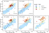 |
Fig. 1. Observed m814−m140 vs. m140−[3.6] colour-colour diagram of candidate cluster members at r/r500 < 0.7 for all clusters, down to the m140 limit indicated in each panel, coded by best-fit Sersic index as indicated in the legend (dark red, green and blue symbols). Filled and empty symbols show, respectively, galaxies above and below the stellar mass completeness limit for the individual cluster (Table 1). Symbol size scales with the statistical background-subtraction weight (Sect. 2.2.1; smaller symbols are overall more likely to be interlopers). In each panel, the black line marks the adopted separation between quiescent and star-forming galaxies, following S19. The background colour scale traces the median Sersic index (see legend) across the colour diagram (within a colour distance of 0.1 mag) of galaxies in the reference field sample with photo-zs within ±0.1 from the cluster’s redshift, and same m140 magnitude limit (only colour bins with at least five galaxies are shown). |
Finally, for these galaxy samples we use the same empirical stellar mass estimates as in S19. These are derived by scaling the 3.6 μm flux5 to stellar mass with a mass-to-light ratio (M/L) based on the m814−m140 colour, as calibrated on stellar masses derived by parametric SED modelling for a reference sample of galaxies at each cluster redshift from the GOODS-S field (full details in Sect. 2.3.1 in S19). The estimated uncertainty on the individual stellar mass estimates deriving from the scatter in this empirical calibration is of order 20−30% – as stressed in S19 this relies on the assumptions adopted to estimate stellar masses for the reference sample, and thus this uncertainty does not correspond to the stellar mass uncertainty on an absolute scale.
In contrast with stellar mass estimates adopted in S19 that were scaled to a “total flux” as estimated by SExtractor (Bertin & Arnouts 1996) FLUX_AUTO, mass estimates used in the following are scaled to total fluxes as measured by T_PHOT in the attempt to more closely recover the whole source flux as also done for the field sample (see Sect. 2.3). Differences on the total flux are ∼10%, implying that stellar mass estimates used in the following are larger than those in S19 by the same amount.
In this respect, we further note that for several aspects of the analyses presented here we compare the cluster galaxy samples with reference field samples in four fields from the CANDELS survey, as discussed in Sect. 2.3. We stress that the stellar masses measured for the cluster galaxy sample as discussed above are not derived in the same way as those for the field reference sample (see Sect. 2.3). While this was also the case for our analysis in S19, the S19 mass estimates were directly calibrated on galaxies from the very same galaxy catalogue in GOODS-S that was also adopted as a control field sample, where we could very closely match the photometry in the relevant bands between cluster and field samples. Instead, in this work we use independent stellar mass and photometric redshift catalogues for the four adopted reference fields from Skelton et al. (2014), as detailed in Sect. 2.3.
The proper comparison of results for cluster galaxies and reference field counterparts relies on the proper comparison of their stellar mass estimates. As there is no overlap between the cluster and field sky areas, we cannot directly compare mass estimates for individual sources. We thus attempt a quantification of the impact of potential systematics in the mass estimates of cluster versus field samples coming from their different measurement procedure (i.e. Skelton et al. 2014 SED-fitting based masses versus empirical estimates adopted for cluster galaxies) and possible systematic offsets in photometric measurements driving stellar mass estimates. We evaluate the impact of the former by computing empirical stellar mass estimates for the Skelton et al. (2014) sources with the same procedure adopted for cluster galaxies, separately for quiescent and star-forming sources and as a function of redshift across the range of interest 1.3 < z < 1.8. This evaluation suggests stellar mass offsets of order ≲10% for galaxies at z < 1.6, and of order ∼10−15% at z > 1.6. In the following, we correct by default the stellar masses of cluster galaxies by the estimated systematics6 to bring them on the same scale of the reference field catalogue, and minimise the impact on the cluster versus field galaxy comparison.
Concerning systematics in the photometry driving stellar mass estimates, although galaxies in both cluster and field samples used in the following analyses are all observed with sufficiently high S/N to limit concerns on the uncertainty of photometric measurements, some differences may occur due to the definition of the adopted total fluxes and/or their actual measurement (also depending on specific characteristics of the images). In the S/N range of interest, we consider such potential systematics very unlikely to exceed a factor ∼10%, and given our adopted empirical estimation of stellar masses discussed above we thus consider the impact of a 0.1 mag systematic on the 3.6 μm flux and/or on the m814−m140 colour, which result in systematics on the estimated stellar mass of about 10% and < 5%, respectively.
The sources of systematics on stellar mass estimates discussed above are largely independent from each other, and we thus estimate that any residual potential systematics affecting stellar masses in the cluster versus field comparisons carried out in the following will stay below the < 20% level overall. We comment in the following on the impact of such potential systematics on our results, as relevant.
For the analyses presented in the following, we consider cluster galaxy samples complete down to a stellar mass limit defined as in S19. A mass completeness limit is computed, for each cluster, as the stellar mass of an unattenuated Bruzual & Charlot (2003) simple stellar population (SSP) of solar metallicity, formed at zf ∼ 8, having at the cluster redshift a F140W-band magnitude equal to the m140 limit adopted for the given cluster (see Table 1). These mass completeness limits for the individual clusters range between log(M/M⊙) = 10.54 − 10.85 across the probed cluster redshift range (see Table 1). The bulk of the analyses presented here refer to the combined cluster galaxy sample across all five clusters, down to a mass completeness limit of log(M/M⊙) = 10.85.
2.3. Field reference
In this work we use a field reference sample from the CANDELS/3D-HST survey fields in GOODS-S, AEGIS, COSMOS, and UDS (Grogin et al. 2011; Koekemoer et al. 2011; Brammer et al. 2012)7. We use specifically multiwavelength photometry and derived photometric redshifts (photo-zs), stellar masses and restframe colours from Skelton et al. (2014), together with parametric morphology measurements from van der Wel et al. (2014), analogous to those performed in the cluster fields as described in Sect. 2.4. Following van der Wel et al. (2014), stellar masses are corrected based on the ratio of the flux in the photometric catalogue used for stellar mass estimation to the total flux as measured by GALFIT in the van der Wel et al. (2014) morphological analysis. For the galaxy sample relevant to this work (that is, within the photo-z and stellar mass range of interest, and within morphological analysis flag constraints as described below) this results in a median correction of stellar masses by ∼6%, with < 1% of galaxies having correction factors larger than 2.
In the following analyses we focus on (various sub-samples of) galaxies with photo-zs in the 1.3−1.8 range and stellar mass above the relevant mass completeness limit for the corresponding cluster galaxy samples, with uniform quality photometry (i.e. use_phot > 0 as defined in Skelton et al. 2014). With this selection, we start from ∼900 galaxies in the combined GOODS-S, AEGIS, COSMOS and UDS sample from the Skelton et al. (2014) catalogues. We then remove sources flagged as bad fits (with bad fits identified by morphology flag f ≥ 2 as defined in van der Wel et al. 2012) in the van der Wel et al. (2014) morphology measurements, which leaves ∼770 galaxies. We further remove from this sample ∼1% of sources with estimated uncertainties on Sersic index or effective radius larger than 20%. The resulting sample with available morphological measurements thus contains 84% of the photo-z and stellar-mass selected sample at log(M/M⊙ > 10.85). Finally, this sample still contains potentially suspicious morphological measurements (morphology flag f = 1, see definition details in van der Wel et al. 2012, 2014), which if removed reduce the field reference sample with morphological measurements to ∼570 galaxies, or 63% of the photo-z and mass selected sample. Apart from lowering as discussed the statistics of the control field sample, we verify that removing these suspicious measurements does not affect the results presented in the following (very few, marginal exceptions are mentioned where relevant). Results and figures in the following are thus presented by default for the clean sample (excluding suspicious measurements).
We classify galaxies from the field reference sample as quiescent vs. star-forming based on restframe UVJ colours from Skelton et al. (2014). We use in particular the Williams et al. (2009) UVJ classification criterion. To limit the impact of the boundary region between the quiescent and star-forming populations in the UVJ colour plane, some results are also quoted excluding from the analysis a band of ±0.1 mag around the dividing line.
Finally, for the analyses below we need in some cases the F140W band magnitude of the reference field galaxies. The depth of the CANDELS F140W-band imaging is shallower than the depth of the F140W data on the cluster fields (∼800 s vs. ≳2400 s per pointing), however in the magnitude range relevant to this work (m140 ≤ 23.5) the S/N of sources is still sufficiently high (> 10 at the faintest end) for all our purposes. However, as the CANDELS fields are only partially covered with F140W imaging (Brammer et al. 2012), for some sources there is no F140W band magnitude available. In such cases (∼40% of the used field galaxy sample at 1.3 < z < 1.8 and log(M/M⊙) > 10.85 or m140 < 23.5), we substitute a m140 proxy based on the (deeper) F160W band magnitude. We calibrate this proxy on sources in the magnitude and redshift range of interest from the F140W-imaged part of the survey, for quiescent and star-forming galaxies separately, which yields a m140−m160 colour term of ∼0.21 mag independent of magnitude for quiescent sources, and between ∼0.2 mag and ∼0.1 mag across the magnitude range of interest for star-forming galaxies. By comparison with sources in the F140W-imaged part of the survey we estimate that, in the magnitude (or mass) and redshift range relevant to this work, our estimated m140 magnitudes have negligible systematic offsets with respect to actually measured ones (within 0.02 mag at most), and a scatter of at most 0.1 mag across the full magnitude range of interest. Over such magnitude range, this scatter is dominated by scatter in the colour term (rather than by F160W band magnitude uncertainty), and it is indeed larger than the estimated uncertainty of the actually measured F140W magnitude for sources where it is available. We thus use actually measured (rather than estimated from F160W) F140W band magnitudes where they are available.
2.4. Morphological analysis of cluster galaxies
We use GALFIT (Peng et al. 2002, 2010) to fit PSF-convolved, single-component Sersic profiles to the galaxy surface brightness distribution in the HST/WFC3 F140W band images, for all sources detected in the cluster fields down to m140 = 24 mag. At the clusters’ redshift, the F140W band images approximately probe the restframe V band.
GALFIT is run on the F140W images in counts units, with a non-zero background (see e.g. Peng et al. 2002), and with pixel scale of 0.03″. An independent PSF model for each of the five cluster fields is created from non-saturated, high-S/N point-like sources selected from the F140W-band source catalogues described in S19. We assess the impact of the adopted PSF model by comparing results obtained with PSF models of the other clusters, or derived from other surveys, or produced from our data but with different procedures. From these comparisons we estimate at most a systematic offset of 5% and 1% for Sersic indices and effective radii, respectively. This level of systematics has negligible impact on the results presented in this work – including concerning Sersic indices, which are only used for a rather broad morphological classification, given the intrinsic scatter and uncertainties in the relation between Sersic index and detailed structural properties. Indeed, in the following we mostly consider three broad morphology classes with Sersic index n < 1.5 (disk-dominated galaxies), n > 2.5 (bulge-dominated galaxies), and the remaining intermediate sources with 1.5 < n < 2.5.
The surface brightness profile of galaxies in the cluster fields is modelled by means of an unsupervised fitting, to limit the introduction of arbitrariness in the procedure. For each source in the F140W-band catalogue satisfying the m140 < 24 mag limit, we model an image area centred on the target and with size depending on the projected dimensions of the target itself (10 times the size estimated from the SExtractor detection, in both x and y directions). The background level is assumed to be constant over the cutout area and is modelled as a free parameter. All objects falling in the cutout area, and down to a limit of 3 magnitudes fainter than the given target, are simultaneously modelled, as well as bright objects outside of the selected region but close and bright enough that their light could produce asymmetric background features. A proper treatment of neighbouring sources is indeed necessary also to allow GALFIT to derive a robust background level, a critical point even for single-Sersic profile fitting, especially for high Sersic index sources having faint extended emission.
To quantify uncertainties on our estimates of morphological parameters, both for individual sources and overall for the galaxy (sub-)populations of interest in this work, we use simulations (injecting artificial sources in the image, with known profile parameters spanning the range of interest) as well as multiple fitting results deriving from objects falling in more than one modelled cutout area. Over the magnitude range relevant to this work (m140 < 23.5), we estimate that typical statistical uncertainties on the measured Sersic index and effective radius are within ∼10% and 5%, respectively, with systematics of < 2% at most at all magnitudes of interest.
With this surface brightness modelling, we obtain measurements of structural parameters (and in particular of the effective radius along the major axis of the galaxy, the Sersic index, and the axis ratio) for 94% (97%) of the magnitude (stellar mass, respectively) limited samples above the magnitude (mass completeness) limit adopted for the individual clusters. For the overall mass-complete sample above log(M/M⊙) > 10.85 used for the bulk of the analyses presented here, structural measurements are available for 96 out of 99 galaxies. For consistency with the constraints applied for the measurements in the reference field sample (van der Wel et al. 2014, see below and Sect. 2.3) we also exclude from the analysis a further four sources with n > 8 (specifically, 8 < n < 13) above the log(M/M⊙) > 10.85 limit8. This has no relevant impact on the results presented here, which would remain well within the quoted uncertainties if these four sources were included.
In many analyses presented in the following, we rely on the comparison of structural properties of cluster galaxies to those of field counterparts from a control field. As described in Sect. 2.3, for this purpose we use morphological measurements published in van der Wel et al. (2014). Although the adopted parametric modelling in this work and in van der Wel et al. (2014) is similar, a number of details in the adopted procedures, as well as in the reduction and analysis of the imaging data, may potentially introduce biases in the measurements used in the following, especially in the more sensitive parameter estimates, namely Sersic indices and effective radii. As there is no overlap between the cluster and control fields, in an attempt to quantify such potential biases and assess their impact on our results, we reduce and analyse a limited portion of the control field imaging data, and carry out the morphological analysis with exactly the same procedures that we adopted for the cluster fields. We then compare our results with the van der Wel et al. (2014) measurements we use in the following, as detailed in Appendix A. Based on that comparison, our estimated effective radii for the overall galaxy population in the magnitude range considered here, as well as split by star-forming and quiescent sources, might be at face value slightly biased towards lower values with respect to van der Wel et al. (2014), by < 5% for the overall population in the probed magnitude range. As it could be expected, such a bias might depend on the Sersic index of the source (at face value, increasing from ∼3% up to ∼8% for low- to high-Sersic index galaxies, see Appendix A). We specifically consider the impact of this potential bias on our results on the environmental dependence of galaxy sizes in Sect. 3.2.
Concerning Sersic indices, based on this comparison our estimates for the whole population in the considered magnitude range might be biased by ∼4% towards lower values with respect to van der Wel et al. (2014). Also here there might be potential – but of marginal significance with the estimated uncertainties – dependence of the bias on the Sersic index (anyway at the < 7% level for all sub-populations, see Appendix A). The impact of such bias on the results presented in the following is always well within the estimated statistical uncertainties, and it is in fact in most cases unnoticeable. Therefore, we consider it negligible for the purposes of this work, and all results presented in the following are shown for our estimated Sersic indices with no corrections.
Based on the comparison discussed above, we estimate that any residual systematics between cluster and field galaxy samples on both effective radii and Sersic indices will not exceed the ∼5% level. We comment where relevant in the following on the impact of potential systematics at such level on the presented results.
In the following, galaxy sizes are intended as effective radii, and we adopt specifically the semi-major axis of the ellipse containing half of the total flux of the best-fitting Sersic model. The average restframe wavelength across the probed redshift range, corresponding to the F140W band imaging where cluster galaxy sizes are determined, is 5500 Å. For the field galaxy sample, we adopt sizes from van der Wel et al. (2014) measured in the F160W band, for which the average restframe wavelength across the probed redshift range is 6270 Å. To account for the wavelength dependence of galaxy sizes, all sizes discussed in the following for both cluster and field samples are scaled to a restframe wavelength of 5500 Å. For this purpose, we proceed more specifically as follows: to scale the measured size to 5500 Å restframe, we adopt the relevant scalings of size as a function of wavelength as given in van der Wel et al. (2014) for both quiescent and star-forming galaxies. In general, we use the quiescent or star-forming scaling for galaxies that are classified as quiescent or star-forming, respectively. For galaxies within ±0.1 mag from the colour separation between quiescent and star-forming sources, we adopt the scaling for quiescent (star-forming) galaxies based on their Sersic index being larger (smaller, respectively) than 2. For a minority of sources (∼10% and 20% of the log(M/M⊙) > 10.85 field and cluster galaxy samples, respectively) we adopt instead the alternative scaling with respect to that determined with these criteria, based on their measured sizes. More specifically: we first determine the “reference size” of each source, as the size corresponding to its stellar mass and photo-z according to the van der Wel et al. (2014) mass-size relation for quiescent and star-forming galaxies, scaled to the observed wavelength (F140W for cluster galaxies, F160W for field galaxies). Then, for sources where the quiescent galaxy scaling should be adopted based on the aforementioned criteria, but whose sizes are larger than a factor 2x their supposed reference size and closer to the star-forming mass-size relation, we use the scaling for star-forming galaxies – and conversely for star-forming sources smaller than 2x their reference size. We stress that, as also described in van der Wel et al. (2014), we apply these corrections with the aim of limiting the introduction of systematic biases, but given the small redshift range of interest and the chosen 5500 Å reference wavelength being close to the observed wavelength, corrections are small. For the cluster galaxy sample, all corrections for individual galaxies are within 3%, and average corrections across the five clusters go from ∼0.2% to ∼1.5% depending on the cluster redshift. For field galaxies in the relevant mass and redshift range, corrections range from ∼1% to ∼10% with an average correction of 4% and > 90% of the galaxies having corrections < 8%.
3. Structural properties of cluster galaxies
In the following we combine the S19 measurements summarised in Sect. 2 with the morphological analysis described in Sect. 2.4. We focus in particular on the relation between broad structural and stellar population properties, and environmental dependence of galaxy morphologies, in Sect. 3.1, and on the stellar mass–size relation and environmental dependence of galaxy sizes in Sect. 3.2.
In the analyses described in this Section we often mark or exclude as it is customary the cluster brightest central galaxies (BCGs), because of their intrinsically peculiar nature that may be reflected in their structural properties. As detailed in S19, BCGs are identified in each cluster as the brightest red galaxy9 within a distance of 100 kpc (proper) from the projected number density peak of candidate members (Fig. 4 in S19). The adopted BCG is thus the brightest red – and most massive, with stellar masses in the range 2 × 10¹¹–1012 M⊙ – galaxy at the centre of the red galaxy concentration associated with the cluster (see S19 for more details). All BCGs in this cluster sample are classified as quiescent galaxies. Their median Sersic index is ∼5 (with individual estimates in the range n ∼ 3 − 6). Estimated BCG sizes range from ∼3 to ∼15 kpc, with an average size of ∼9 kpc. We note that, as discussed in S19, the adopted BCG is also the most massive galaxy of the whole candidate member sample in all clusters except SPT-CLJ0459 (where six formally more massive – by factors 5% to 70% – sources are spread along the galaxy overdensity). Furthermore, in SPT-CLJ0446 and SPT-CLJ0459 a similarly massive, bulge-dominated, quiescent galaxy identified as a very likely cluster member is found within a distance of < 7 kpc. In such cases of “double BCG” the BCG definition is arbitrary to this extent, but this does not affect any of the results presented here.
We further note that, for what is relevant to the purposes of this analysis, we cannot identify significant deviations between the cluster and field galaxy stellar mass distributions in the probed mass range. Although there could be a mild overabundance of the most massive galaxies in clusters with respect to the field population (largely due to BCGs), its significance with the uncertainties and sample statistics available in this work is marginal.
3.1. Morphological properties of cluster galaxy populations
Figure 1 shows the m814−m140 vs. m140−[3.6] colour-colour diagram (as a proxy of the restframe UVJ diagram, as discussed in Sect. 2.2.2) of candidate cluster members. Colours of cluster members in this diagram, as well as the separation between star-forming and quiescent galaxies, follow S19 (their Fig. 6, see Sect. 2.2.2). In Fig. 1, candidate members are coded according to their best-fit Sersic index, dividing the overall population into low, intermediate and high-Sersic index sources. The background colour shading shows the median Sersic index of field counterparts across the diagram10.
The distribution of galaxies in Fig. 1 reflects the known correlation between broad stellar population and structural properties, with quiescence and active star formation preferentially occurring in high-Sersic index (“bulge-dominated”) and disk-dominated structures, respectively. As shown in Fig. 1, in general terms this correlation occurs similarly in both cluster and field galaxy samples.
We quantify this correlation by investigating the morphology mix of different galaxy sub-populations in the cluster and reference fields. For this purpose, we combine all five clusters and only consider galaxies above the common mass completeness limit of log(M/M⊙) = 10.85. We then select a field comparison sample at 1.3 < z < 1.8 and with the same stellar mass limit. Figure 2 (left) shows the fraction of galaxies with Sersic index n ≤ 1.5, 1.5 < n < 2.5 and n ≥ 2.5 among the full population of log(M/M⊙) > 10.85 cluster galaxies, as compared to the analogous fractions in the field reference sample.
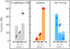 |
Fig. 2. Morphology mix of massive galaxies in the probed cluster regions and in the reference field at 1.3 < z < 1.8. Left panel: fraction of log(M/M⊙) > 10.85 cluster galaxies with Sersic indices n ≤ 1.5, 1.5 < n < 2.5 and n ≥ 2.5 (dark grey symbols), and the corresponding fractions for the field reference sample (grey bars). For clarity, error bars (binomial, Cameron 2011) are only shown for cluster samples. Right panel: analogous fractions for the quiescent and star-forming populations, as indicated. Solid (empty) symbols refer to cluster galaxy samples excluding (including) sources within ±0.1 mag around the quiescent vs. star-forming classification border. Solid (hatched) bars analogously refer to the corresponding field reference samples. |
Figure 2 (left) shows that the morphology mix of the massive galaxy population in the probed cluster regions is skewed towards bulge-dominated systems with respect to the field, showing that a morphology-density relation is already in place in these environments.
On the other hand, the right-hand panel of Fig. 2 shows that the morphology mix of the separate quiescent and star-forming populations in cluster versus field environments is in fact fully consistent. Therefore, the morphology-density relation in the left-hand panel is largely connected to the higher quiescent fraction in the cluster galaxy population with respect to the field.
Figure 2 (right) also quantifies more specifically the correlation between broad structural and stellar population properties in the probed stellar mass range, with ∼80% of quiescent galaxies being bulge-dominated (n > 2.5) sources, whereas ∼60% of star-forming galaxies are disk-dominated (n < 1.5), in both cluster and field environments. Likewise, the vast majority of bulge-dominated galaxies is quiescent ( % and 77 ± 3% in the cluster and field samples, respectively11), while disk-dominated sources are predominantly (∼80−90%) star-forming.
Fractions for cluster galaxy samples in Fig. 2 are based on all candidate members weighted as described in Sect. 2.2.1 to account for residual background contamination. Such contamination amounts to ≲-pagination10% for all quiescent samples (including Sersic index selected sub-samples), to typically 40−50% for star-forming samples, and to almost 20% for the overall full population, going from 13% for n > 2.5 sources to 35% for n < 1.5. As also shown in Fig. 2, the impact of excluding a region of ±0.1 mag around the star-forming vs. quiescent classification border is typically marginal (and largely within the estimated uncertainties) for both cluster and field samples. The impact of matching the redshift distribution of the field sample to that of the cluster galaxy sample (which is made of three spikes at z ∼ 1.4, 1.5 and 1.7) is also marginal (< -pagination10% differences) and in any case within the statistical uncertainties. The impact of residual systematics on the Sersic index at the level described in Sect. 2.4, and of potential residual systematics on stellar masses as discussed in Sect. 2.2.2, is largely negligible and remains anyway well within the uncertainties shown in Fig. 2.
We note that with these observations our classification of quiescent vs. star-forming galaxies is necessarily broad in nature, and cannot identify recently quenched, transition sources in any reliable nor statistically meaningful way. Furthermore, focusing on the relatively central cluster regions implies that our cluster galaxy samples are dominated by sources accreted onto the cluster at earlier epochs. For these reasons, a potential environmental signature more noticeable only on recently quenched galaxies might involve a minority population in our samples, with no clear identification, and might thus go undetected in our analysis. Furthermore, our analysis focusses on massive galaxies, while more significant signatures might be visible at lower masses (e.g. Chan et al. 2021), possibly in relation to a potential mass dependence of environmental quenching mechanisms in clusters at this redshift, as discussed in e.g. van der Burg et al. (2020), Baxter et al. (2022). However, according to these studies the environmental quenching efficiency is higher for more massive galaxies; therefore, the stellar mass regime probed here should, in that respect, facilitate the detection of signatures related to environmental quenching. We further note that the Sersic index classification adopted here to separate bulge- vs. disk-dominated galaxies has known limitations and might also possibly affect the detection of specific signatures. Nonetheless, these observations show no obvious environmental signatures in the correlation between broad structural and stellar population properties as probed here, suggesting a connection between environmental quenching and structural evolution on timescales smaller than we can disentangle with this analysis.
The average Sersic indices for quiescent versus star-forming cluster galaxies above the log(M/M⊙) > 10.85 stellar mass limit, all clusters combined and accounting for background contamination, are n = 3.8 ± 0.2 and n = 1.3 ± 0.2, respectively (uncertainties are determined by bootstrap, BCGs are excluded). Corresponding values for the field reference sample above the same mass limit are n = 3.49 ± 0.09 and 1.50 ± 0.07 at 1.3 < z < 1.8, with no significant variation across this redshift range. We note though that including suspicious sources (see Sect. 2.3) gives average Sersic indices of, respectively, n = 3.76 ± 0.09 and 1.66 ± 0.07. Although there might be small differences in the average Sersic indices of quiescent and star-forming cluster galaxies versus field counterparts, they are minor and cannot be considered significant given the estimated measurement uncertainties.
As a further probe of potential environmental signatures on the morphology of the quiescent galaxy population related to environmental quenching, we compare in Fig. 3 the axis ratio distribution of massive (log(M/M⊙) > 10.85) quiescent galaxies in the cluster and field (1.3 < z < 1.8) samples. As in Fig. 2, all candidate cluster members are shown, weighted as described in Sect. 2.2.1 to account for residual background contamination. Excluding sources within ±0.1 mag around the quiescent vs. star-forming classification border does not affect the result, as shown. Figure 3 does not show any significant difference between the axis ratio distributions of quiescent galaxies in the cluster versus field samples (as also confirmed by K-S test, both including and excluding sources around the classification border). As mentioned in Sect. 1, different studies found seemingly contrasting results on this aspect. In particular at redshifts bracketing the range of clusters studied here, Newman et al. (2014, at stellar masses log(M/M⊙) > 10.8, in the massive cluster JKCS 041 at z = 1.8) highlighted a lack of flattened, oblate quiescent galaxies in cluster versus field samples, whereas Chan et al. (2021, 11 clusters at 1 < z < 1.4 from the GOGREEN survey) found an excess (but most remarkably at lower masses, 10.4 < log(M/M⊙ < 10.8). We show in Fig. 3 a rendition of the Chan et al. (2021)12 axis ratio distribution of massive, quiescent cluster galaxies (hatched region, corresponding to the 1σ range around the weighted average13). Although this rendition suggests that Chan et al. (2021) results are largely consistent with our determination in this stellar mass range, our axis ratio distribution might be somewhat less skewed towards very high axis ratios, albeit the significance of this difference is marginal given the estimated uncertainties. We note though that Chan et al. (2021) find that the most noticeable environmental signatures on the axis ratio distribution of quiescent galaxies is found at lower stellar masses than those probed here.
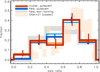 |
Fig. 3. Distribution of axis ratios of log(M/M⊙) > 10.85 quiescent cluster galaxies in the probed cluster regions across the whole cluster sample (red shades) and in the reference field at 1.3 < z < 1.8 (blue shades, as indicated). For both cluster and field samples, darker (lighter) lines correspond to excluding (including) sources within ±0.1 mag around the quiescent vs. star-forming classification border. Error bars on the fractions over the whole population (binomial, Cameron 2011) are slightly offset for clarity. For comparison, the axis ratio distribution of star-forming field galaxies in the same mass and redshift range (grey line, errors within line width), and for 1 < z < 1.4 cluster galaxies in the same stellar mass range from Chan et al. (2021, hatched region, see text for details) are also shown. |
3.2. The stellar mass-size relation
As discussed in Sect. 2.4, we find a (small) bias between size measurements in the cluster and control field samples. Given the direct impact of such bias on results presented here, in the following we apply a correction to the measured sizes of cluster galaxies to bring them on the same scale as the reference field measurements. We specifically comment as needed on the impact of this correction on the results.
Figure 4 shows the stellar mass – size relation of selected galaxy populations in both the combined cluster and field samples. To combine all sources into one figure limiting the impact of redshift-dependent effects, all galaxy sizes are scaled to a common redshift of z = 1.5 for the purpose of this figure, using the redshift evolution14 of the mass-size relation for star-forming and quiescent galaxies as determined in van der Wel et al. (2014). Cluster and field samples are split based on Sersic index into disk-dominated (n ≤ 1.5), intermediate (1.5 < n < 2.5) and bulge-dominated (n ≥ 2.5) sources, and coded according to their quiescent vs. star-forming classification.
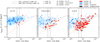 |
Fig. 4. Stellar mass – size relation of candidate cluster members and field counterparts, split by Sersic index as indicated. All candidate members in the m140-limited samples across the five clusters are shown, with symbol size scaling with residual statistical background subtraction weights (Sect. 2.2.1). All sizes for both candidate members and field counterparts are scaled to a common redshift z = 1.5 for the purpose of this figure (see text). Candidate cluster members are shown with darker symbols, colour-coded by quiescent (red) vs. star-forming (blue) classification (purple and black symbols show, respectively, galaxies within ±0.1 mag from the classification border, and with no reliable classification). Large grey open squares indicate cluster BCGs (right hand panel). Light blue and light red squares in the background show counterparts from the control field sample at 1.35 < z < 1.75. The red and blue lines show the best-fit mass-size relations for quiescent and star-forming galaxies from van der Wel et al. (2014, also scaled to z = 1.5). Vertical grey lines mark the minimum and maximum stellar mass completeness limits across the five clusters. |
Figure 4 shows a substantial similarity in the mass-size relation of cluster and field galaxies, and highlights again the clear correlation between broad structural and stellar population properties discussed in Sect. 3.1. We note in particular that star-forming and quiescent cluster galaxy populations largely follow the respective van der Wel et al. (2014) mass-size relations determined for field galaxies. Estimating a best-fit mass-size relation for quiescent cluster galaxies from the data in Fig. 4, assuming a linear form in log(size) vs. log(mass) in the probed mass range log(M/M⊙) > 10.85, would give a best-fit relation within 5% of the adopted determination based on van der Wel et al. (2014), and fully consistent within the estimated uncertainties15. In the following we thus use the van der Wel et al. (2014) relations as a reference, in quantifying size differences between cluster galaxies and field counterparts.
The distribution of the selected subpopulations in the mass-size plane is remarkably similar in the cluster and field environments, the most noticeable difference occurring for intermediate Sersic index sources, for which larger, typically star-forming galaxies are underrepresented in clusters with respect to the field. Although this would be potentially very interesting in relation to the investigation of the correlation and timescales of star formation quenching and structural evolution in cluster versus field environments, we note that at least part of this effect might be due to the combination of uncertainties in the estimated Sersic indices and the higher quiescent fraction in the cluster versus field samples. This combination results in a larger number of star-forming (thus largely disk-dominated, and larger in size) galaxies being scattered into the intermediate-n sub-sample for the field, whereas a larger number of quiescent (thus largely bulge-dominated, and smaller in size) galaxies are scattered into the intermediate-n sub-sample for the clusters. Indeed, as noticeable in Fig. 4, the quiescent galaxy fraction in the intermediate-n sample is tendentially higher in clusters than in the field, though with marginal significance with the given uncertainties (∼60 ± 15% vs. 40 ± 10%). Although for the reason just discussed we refrain from elaborating on this further, we note that this is qualitatively similar (quantitative comparison is affected by the different stellar mass range probed) to what observed in z ∼ 1 clusters by Matharu et al. (2019, see also references therein).
In Fig. 5 we show the median size difference16 of cluster and field galaxies more massive than log(M/M⊙) = 10.85, adopting as a reference the van der Wel et al. (2014) best-fit mass-size relations for star-forming (left panel) and quiescent (right panel) galaxies. For each galaxy in the combined cluster and in the control field samples, we estimate the log difference of the measured size with respect to the expected size from the van der Wel et al. (2014) relations17 for a galaxy of the given stellar mass and redshift (for cluster galaxies, the cluster redshift is assumed).
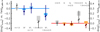 |
Fig. 5. Median log size difference of log(M/M⊙) > 10.85 cluster galaxies (darker symbols with error bars, corrected for residual background subtraction, see text) and of field counterparts at 1.3 < z < 1.8 (shaded rectangles showing the 16th–84th percentile range, see text) with respect to the expected size from the van der Wel et al. (2014) star-forming (left panel) and quiescent (right panel) relations. Median differences are shown for different sub-samples based on Sersic index (symbols as in Fig. 4, or squares for no Sersic index selection) and star-forming (blue colour shades) vs. quiescent (red colour shades) classification (grey symbols show samples selected by Sersic index only, regardless of star-forming vs. quiescent classification; see text). |
Given the intrinsic variety within, and overlap between, colour – and morphology – selected galaxy populations, in order to probe the potential effect of galaxy sample selection on the identification of environmental signatures on galaxy sizes, we consider for both cluster and field samples several galaxy sub-samples (always excluding BCGs). As shown in Fig. 5, we divide the population according to Sersic index (n < 1.5, 1.5 < n < 2.5, n > 2.5) and star-forming vs. quiescent classification (to limit differential contamination issues between the quiescent and star-forming populations along the border of the UVJ-like classification in cluster versus field samples, Fig. 5 shows results excluding the ±0.1 mag around the star-forming vs. quiescent classification border, but the impact of this removal remains well within the 1σ uncertainties for all measurements shown, and has no impact on the results). For each sub-sample, we compute for both cluster and field populations the median log difference of the measured galaxy size with respect to the expected size. To account for background contamination of the cluster candidate member sample, for each sub-sample we estimate the expected number of contaminants based on the statistical weights described in Sect. 2.2.1, and randomly remove the estimated number of interlopers according to the size distribution of the corresponding field sub-sample. The uncertainties shown in Fig. 5 for both cluster and field median size offsets with respect to the van der Wel et al. (2014) mass-size relations are estimated from the 16th–84th percentile range of the distribution of median size offsets obtained by bootstrapping 10 000 times for each sub-sample. The quoted uncertainties thus reflect Poisson noise given the sample size, and background contamination removal for cluster galaxy samples. We note that, given the lack of evidence for a redshift dependence of the median size offset of the control field sample (see Fig. A.4) we do not match the redshift distribution of field galaxies to that of the cluster galaxy sample, but use instead the whole selected field sample in the 1.3 < z < 1.8 range.
Figure 5 shows that for all considered sub-samples the median size offsets of cluster and field galaxies with respect to the reference relations are generally consistent18 according to the statistical uncertainties estimated as above. Cluster versus field galaxy size median differences are within ∼10% (see Fig. 6) for all considered subpopulations with the exception of intermediate Sersic index sources, where cluster galaxies might be at face value smaller than field counterparts, but average sizes are still consistent given the significant uncertainties. Figures 4 (middle) and 5 show that this effect, if real, would largely be due to the different composition of the cluster and field intermediate-n samples (see earlier discussion on Fig. 4), with a larger fraction of star-forming – and thus typically larger – sources in the field sample increasing the average size of intermediate-n field galaxies with respect to cluster analogues. However, as discussed above in relation to Fig. 4, this is at least partly due to the higher quiescent fraction in the cluster versus field populations, producing a differential contamination of the intermediate-n samples. Also in consideration of the significant statistical uncertainty that anyway affects this estimated size difference, we thus do not comment further on this potential difference in the following.
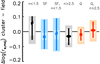 |
Fig. 6. Median log size difference between cluster and field galaxies as derived from Fig. 5, for different population sub-samples (see text). Symbols and colour coding follow Fig. 5. Error bars show statistical uncertainties (including statistical background subtraction). Light shaded rectangles show the maximum impact on the median difference from potential residual uncorrected systematics. Dark shaded rectangles show the combined error including both statistical and systematic uncertainties (see text). |
The general similarity of sizes of cluster and field galaxies in Fig. 5 is reflected in Fig. 6 that quantifies more explicitly the median size difference of cluster versus field galaxies, as derived from the results in Fig. 5. We focus here on six most relevant sub-samples, concerning the bulk of star-forming (disk-dominated galaxies, star-forming galaxies, and star-forming disk galaxies) and quiescent populations (bulge-dominated galaxies, quiescent galaxies, and quiescent bulge-dominated galaxies). Thin error bars show statistical errors (as derived from bootstrap as discussed above for Fig. 5). We estimate the possible impact of potential residual systematics on stellar masses, effective radii and Sersic indices (as discussed in Sects. 2.2.2 and 2.4, respectively) by applying random combinations of such systematics up to the estimated maximum level discussed in the relevant Sections, and evaluating the impact on the estimated median size difference between cluster and field galaxies, which is shown as the lighter thick error bar in Fig. 6. The darker thick error bar shows the estimated overall uncertainties (adding in quadrature the statistical and systematic error contributions).
From Fig. 6 we conclude that we see no evidence of a size difference between massive cluster and field galaxies with these observations in the probed redshift and cluster mass range, and in the probed cluster regions. On the other hand, we note that potential differences of up to ∼15% remain within our 1σ uncertainties even for our better-constrained quiescent samples (and up to 20−25% if including our estimate of potential unaccounted systematics; for star-forming galaxies our measurements are even less constraining, as shown in Fig. 6).
4. Summary and conclusions
We investigate structural properties of galaxy populations in the central regions of five of the most massive known clusters at 1.4 ≲ z ≲ 1.7. This cluster sample is homogeneously selected from the wide-area SPT-SZ Sunyaev Zel’dovich effect survey, and it is deemed to be representative of the general population of very massive (M200 > 4 × 10¹⁴ M⊙) clusters at this cosmic time.
With a dedicated, homogeneous imaging follow-up from HST and Spitzer, we probe the connection between broad structural and stellar population properties. We find that a clear relation between the two is already in place at this epoch in these cluster environments, which is in line with several studies in the field up to a similar redshift (e.g. Wuyts et al. 2011; Bell et al. 2012; Kawinwanichakij et al. 2017; Suess et al. 2021, see discussion in Sect. 1). In the probed stellar mass range (log(M/M⊙) > 10.85), quiescent galaxies in both cluster and field environments are largely (∼80%) dominated by bulge-dominated sources, while star-forming galaxies are typically (∼60%) disk-dominated.
Although the morphology mix of both the quiescent and the star-forming populations is largely the same in clusters and in the field, the larger quiescent galaxy fraction observed in these clusters (S19) is reflected in a significant morphology-density relation, with bulge-dominated galaxies already clearly dominating the massive galaxy population in these clusters at z ∼ 1.5.
On the other hand, in the probed stellar mass range, we do not detect any significant environmental dependence of the broad structural properties of quiescent galaxies, which overall show a similar fraction of bulge- versus disk-dominated sources, similar average Sersic indices, as well as a similar axis ratio distribution in the probed cluster and field environments. As discussed in Sect. 3, the analysis presented here is affected by intrinsic limitations that might impact the detection of potential environmental signatures. Indeed, the adopted photometric classification of quiescent versus star-forming galaxies is rather broad in nature, and totally lacks the ability of robustly identifying recently quenched galaxies transitioning towards the quiescent population. Similarly, the classification of bulge- versus disk-dominated systems based on the Sersic index is also inherently broad. Furthermore, this work focusses on the cluster central regions, which are dominated by sources that are accreted onto the cluster at earlier epochs. These limitations may thus affect our ability to detect signatures that might be mostly visible in more recently accreted, recently quenched populations. Nonetheless, the results from this analysis show no significant environmental signatures in the correlation between broad structural and stellar population properties, thus suggesting that a tight connection between star formation quenching and structural evolution towards a bulge-dominated morphology also holds in central cluster regions at this redshift. Any differences in timescales between these two processes in cluster versus field environments are smaller than we can disentangle with this analysis and these observations.
We further probe the stellar mass–size relation of cluster galaxies, finding that star-forming and quiescent cluster galaxy populations largely follow the same relations as their field counterparts. When dividing the population according to the estimated Sersic index, we find that cluster galaxies populate the mass-size plane similarly to field counterparts. A possible exception might be sources with intermediate Sersic index, for which cluster galaxies might tend to be smaller on average due to a larger contribution of quiescent – and thus smaller – sources; see discussion in Sect. 3.2. We estimate the size difference at fixed stellar mass between analogously selected cluster and field galaxies for different sub-populations. With our measurements, we do not find any significant size difference for any of the probed populations. On the other hand, in relation to the results from previous studies (e.g. Andreon 2018; Matharu et al. 2019, see more references and a discussion in Sect. 1), we note that potential differences of ≲-pagination15% are within our estimated statistical uncertainties (1σ; and up to 20−25% if including potential systematics, as discussed in Sect. 3.2), even for the best constrained sub-populations.
This work benefits from a large sample of candidate cluster members, which is unusual for studies of cluster galaxies at this redshift, and it was made possible in this case by the small yet sizeable sample of clusters and by their high mass, implying high richness. These improved statistics result in a better constrained cluster versus field comparison with respect to previous studies at a similar redshift that rely on single and/or lower mass clusters.
Nonetheless, some of our results remain affected by limitations, as discussed above, including – in particular – the relatively coarse characterisation of both structural and stellar population properties, the limited field of view of the observations probing only relatively central cluster regions, and residual uncertainties related to cluster membership especially for some of the probed sub-populations, as discussed. We strive to obtain additional follow-up observations to improve on these specific aspects, thus better exploiting the characteristics of this cluster sample to investigate the interplay between star formation quenching and structural evolution in connection with environmental effects, which is a crucial aspect of galaxy evolution within the most massive structures.
Overdensity radii r500 and r200 quoted in the following are the cluster-centric radii within which the mean density is 500 and 200 times, respectively, the critical density of the Universe at the cluster redshift. The cluster masses M500 and M200 refer to the mass enclosed within these radii.
Following S19, the adopted definition of cluster centre is the position of the brightest red galaxy within 100 kpc (proper) of the projected number density peak of candidate cluster members. The adopted cluster centre thus corresponds to the most massive galaxy lying at the centre of the red galaxy concentration associated with the cluster. See Sect. 3.4 in S19 for full details.
To remove stars from our samples, point-like sources were identified based on the SExtractor’s MAG_AUTO (“total magnitude”) vs. FLUX_RADIUS sequence, down to a F140W band magnitude m140 = 22 mag. This is a purely morphological criterion and thus unresolved non-stellar sources might be misclassified, but as discussed in Sect. 2.1 of S19, the contamination from non-stellar objects of our sample of 120 removed point-like sources across all five clusters is at most at the few percent level.
The colour selection in the m814−m140 vs. m140−[3.6] diagram is different from cluster to cluster because, being based on observed colours, it is redshift dependent. The actual selection adopted for each cluster is shown in Fig. 1.
In a minority of cases where a reliable measurement of the 3.6 μm flux is not available, stellar masses were estimated by scaling the F140W band flux with a M/L ratio calibrated on the m814−m140 colour. The uncertainty on such estimates deriving from the empirical calibration is ∼30−40%. These F140W-flux based masses are only used for a very small fraction of sources in the mass complete samples used in the following, and any small related systematic with respect to the 3.6 μm-flux based masses does not appreciably affect our results, as discussed in Sect. 2.3.1 of S19.
The corrections are estimated as a function of redshift, and for quiescent and star-forming sources, separately. The applied corrections turn out to be as follows: at z < 1.45 (i.e. for SPT-CLJ0421 and SPT-CLJ0607), all mass estimates are increased by 0.01 dex; at 1.45 < z < 1.6 (i.e. for SPT-CLJ2040 and SPT-CLJ0446) mass estimates are decreased by 0.04 and 0.06 dex for quiescent and star-forming galaxies, respectively; at z > 1.6 (i.e. for SPT-CLJ0459), mass estimates are decreased by 0.04 dex and increased by 0.07 dex for quiescent and star-forming galaxies, respectively.
The GOODS-N field is not included because of the lack of F814W band imaging. This allows us to keep the photometric coverage for the field reference sample as close as possible to the one used for the cluster galaxy sample.
A total of 17 sources with n > 8, out of 321 with available structural measurements in the combined magnitude-limited samples across all clusters, are excluded from the analysis.
In fact, the BCG identification is not affected by the specific choice of red colour selection (we formally considered m814−m140 > 1.5), because the adopted BCG is the brightest candidate member – irrespective of colour – in the considered < 100 kpc region. The colour-magnitude diagrams in the whole field probed in these clusters, shown in Fig. 1 of S19, indeed show no blue candidate members brighter than the brightest red galaxies.
In Fig. 1 we show field sources with van der Wel et al. (2014) morphology fit quality flags f = 0 (see Sect. 2.3). Including also sources with f = 1 does not affect the figure appreciably. Furthermore, a small fraction of the overall reference field area is not covered by F814W imaging (and it is thus not included in Fig. 1), corresponding to ∼10% of the total photo-z and m140-selected sample relevant to this figure.
With this analysis and in the probed stellar mass range, we do not find an excess of star-forming early-type galaxies in clusters with respect to the field at this redshift (as found in e.g. Mei et al. 2022), with our estimated star-forming fraction for cluster early-types being if anything somewhat lower than for field counterparts (we note however the differences in stellar mass range, definitions and methodologies between the two studies).
A similar comparison with Newman et al. (2014) results is heavily affected by their small sample size resulting in large statistical uncertainties that prevent the investigation of subtle differences.
Chan et al. (2021) present axis ratio distributions in four stellar mass bins in the range log(M/M⊙)∼9.8 − 12. Their two highest-mass bins overlap with our sample. We show a weighted average of their axis ratio distribution in their two most massive bins, weighting according to the actual contribution of galaxies in these mass ranges in our sample.
For each galaxy, we scale sizes to z = 1.5 based on the van der Wel et al. (2014, their Fig. 6) relations for quiescent or star-forming galaxies, adopting the star-forming or quiescent scaling based on the same criteria described in Sect. 2.4 to scale sizes to 5500 Å restframe.
Although there might be evidence of possible deviations at lower stellar masses, with sizes of quiescent cluster galaxies potentially lying at face value preferentially above the best-fit relation, due to the characteristics of the current observations (Sect. 2) and the possible related biases on the results we do not explore this regime in this work. We leave any related analysis to future investigations with data properly suited to investigate lower-mass populations.
As stated throughout, size measurements of cluster galaxies considered here are corrected by the estimated systematic offset with respect to the adopted control field measurements, as discussed in Sect. 2.4. For the sake of completeness, we show for reference the corresponding measurements of the median size difference of cluster versus field galaxies without this correction in Fig. A.4.
The van der Wel et al. (2014) relations are scaled to sizes at 5500 Å restframe, for consistency with the adopted measurements (see Sect. 2.4).
A K-S test further confirms that the distributions of size offsets of cluster and field galaxies with respect to the reference relations are consistent. A two-sample K-S test is carried out for all sub-populations shown in Fig. 5, with 10 000 realisations for each sub-population to statistically remove background contamination as discussed above. From these tests, the cluster and field samples are consistent with being drawn from the same distribution in 100% of the 10 000 realisations for all sub-populations except the n < 1.5 (90%), star-forming (97%) and 1.5 < n < 2.5 star-forming (83% of the realisations) samples.
Acknowledgments
M.P. and V.S. acknowledge support by the German Space Agency (DLR) through Verbundforschung project ID 50OR1603, and by the German Research Foundation (DFG) through research grant STR 1574/1-1. A.S., M.P. and V.S. acknowledge support by the ERC-StG “ClustersXCosmo” grant agreement 716762. A.S. acknowledges support by the FARE-MIUR grant ‘ClustersXEuclid’ R165SBKTMA, and by the INFN InDark grant. C.L.R. acknowledges support from the Australian Research Council’s Discovery Projects scheme (DP200101068). The South Pole Telescope is supported by the National Science Foundation through grants PLR-1248097, OPP-1852617, and OPP-2147371. Based on observations made with the NASA/ESA Hubble Space Telescope under program GO-14252, obtained from the Data Archive at the Space Telescope Science Institute, which is operated by the Association of Universities for Research in Astronomy, Inc., under NASA contract NAS 5-26555. Based on observations made with the Spitzer Space Telescope (program ID 12030) which is operated by the Jet Propulsion Laboratory, California Institute of Technology under NASA contract.
References
- Afanasiev, A. V., Mei, S., Fu, H., et al. 2022, A&A, in press, https://doi.org/10.1051/0004-6361/202244634 [NASA ADS] [CrossRef] [EDP Sciences] [Google Scholar]
- Alberts, S., Pope, A., Brodwin, M., et al. 2016, ApJ, 825, 72 [NASA ADS] [CrossRef] [Google Scholar]
- Alberts, S., Lee, K.-S., Pope, A., et al. 2021, MNRAS, 501, 1970 [NASA ADS] [CrossRef] [Google Scholar]
- Andersson, K., Benson, B. A., Ade, P. A. R., et al. 2011, ApJ, 738, 48 [NASA ADS] [CrossRef] [Google Scholar]
- Andreon, S. 2018, A&A, 617, A53 [NASA ADS] [CrossRef] [EDP Sciences] [Google Scholar]
- Andreon, S., Maughan, B., Trinchieri, G., & Kurk, J. 2009, A&A, 507, 147 [NASA ADS] [CrossRef] [EDP Sciences] [Google Scholar]
- Andreon, S., Newman, A. B., Trinchieri, G., et al. 2014, A&A, 565, A120 [NASA ADS] [CrossRef] [EDP Sciences] [Google Scholar]
- Baldry, I. K., Balogh, M. L., Bower, R. G., et al. 2006, MNRAS, 373, 469 [Google Scholar]
- Balogh, M. L., Baldry, I. K., Nichol, R., et al. 2004, ApJ, 615, L101 [Google Scholar]
- Bassett, R., Papovich, C., Lotz, J. M., et al. 2013, ApJ, 770, 58 [Google Scholar]
- Baxter, D. C., Cooper, M. C., Balogh, M. L., et al. 2022, MNRAS, 515, 5479 [NASA ADS] [CrossRef] [Google Scholar]
- Bayliss, M. B., Ashby, M. L. N., Ruel, J., et al. 2014, ApJ, 794, 12 [Google Scholar]
- Bell, E. F., van der Wel, A., Papovich, C., et al. 2012, ApJ, 753, 167 [CrossRef] [Google Scholar]
- Bertin, E., & Arnouts, S. 1996, A&AS, 117, 393 [NASA ADS] [CrossRef] [EDP Sciences] [Google Scholar]
- Bleem, L. E., Stalder, B., de Haan, T., et al. 2015, ApJS, 216, 27 [Google Scholar]
- Bocquet, S., Saro, A., Mohr, J. J., et al. 2015, ApJ, 799, 214 [NASA ADS] [CrossRef] [Google Scholar]
- Bocquet, S., Dietrich, J. P., Schrabback, T., et al. 2019, ApJ, 878, 55 [Google Scholar]
- Boselli, A., Roehlly, Y., Fossati, M., et al. 2016, A&A, 596, A11 [NASA ADS] [CrossRef] [EDP Sciences] [Google Scholar]
- Brammer, G. B., van Dokkum, P. G., Franx, M., et al. 2012, ApJS, 200, 13 [Google Scholar]
- Brodwin, M., Gonzalez, A. H., Stanford, S. A., et al. 2012, ApJ, 753, 162 [NASA ADS] [CrossRef] [Google Scholar]
- Brodwin, M., Stanford, S. A., Gonzalez, A. H., et al. 2013, ApJ, 779, 138 [NASA ADS] [CrossRef] [Google Scholar]
- Bruzual, G., & Charlot, S. 2003, MNRAS, 344, 1000 [NASA ADS] [CrossRef] [Google Scholar]
- Cameron, E. 2011, PASA, 28, 128 [Google Scholar]
- Capak, P., Abraham, R. G., Ellis, R. S., et al. 2007, ApJS, 172, 284 [NASA ADS] [CrossRef] [Google Scholar]
- Cappellari, M., Emsellem, E., Krajnović, D., et al. 2011, MNRAS, 416, 1680 [Google Scholar]
- Carlberg, R. G., Yee, H. K. C., Morris, S. L., et al. 2001, ApJ, 563, 736 [NASA ADS] [CrossRef] [Google Scholar]
- Carlstrom, J. E., Ade, P. A. R., Aird, K. A., et al. 2011, PASP, 123, 568 [CrossRef] [Google Scholar]
- Carollo, C. M., Cibinel, A., Lilly, S. J., et al. 2016, ApJ, 818, 180 [NASA ADS] [CrossRef] [Google Scholar]
- Chan, J. C. C., Beifiori, A., Saglia, R. P., et al. 2018, ApJ, 856, 8 [NASA ADS] [CrossRef] [Google Scholar]
- Chan, J. C. C., Wilson, G., Balogh, M., et al. 2021, ApJ, 920, 32 [NASA ADS] [CrossRef] [Google Scholar]
- Cooke, E. A., Hatch, N. A., Stern, D., et al. 2016, ApJ, 816, 83 [NASA ADS] [CrossRef] [Google Scholar]
- de Haan, T., Benson, B., Bleem, L., et al. 2016, ApJ, 832, 95 [NASA ADS] [CrossRef] [Google Scholar]
- de Vaucouleurs, G. 1961, ApJS, 5, 233 [NASA ADS] [CrossRef] [Google Scholar]
- Delaye, L., Huertas-Company, M., Mei, S., et al. 2014, MNRAS, 441, 203 [NASA ADS] [CrossRef] [Google Scholar]
- Di Mascolo, L., Mroczkowski, T., Churazov, E., et al. 2020, A&A, 638, A70 [NASA ADS] [CrossRef] [EDP Sciences] [Google Scholar]
- Dicker, S. R., Romero, C. E., Di Mascolo, L., et al. 2020, ApJ, 902, 144 [NASA ADS] [CrossRef] [Google Scholar]
- Dressler, A. 1980, ApJ, 236, 351 [Google Scholar]
- Finner, K., James Jee, M., Webb, T., et al. 2020, ApJ, 893, 10 [Google Scholar]
- Fioc, M., & Rocca-Volmerange, B. 1999, A&A, 351, 869 [NASA ADS] [Google Scholar]
- Gobat, R., Rosati, P., Strazzullo, V., et al. 2008, A&A, 488, 853 [NASA ADS] [CrossRef] [EDP Sciences] [Google Scholar]
- Gómez, P. L., Nichol, R. C., Miller, C. J., et al. 2003, ApJ, 584, 210 [Google Scholar]
- Goto, T., Yamauchi, C., Fujita, Y., et al. 2003, MNRAS, 346, 601 [NASA ADS] [CrossRef] [Google Scholar]
- Grogin, N. A., Kocevski, D. D., Faber, S. M., et al. 2011, ApJS, 197, 35 [NASA ADS] [CrossRef] [Google Scholar]
- Hayashi, M., Kodama, T., Koyama, Y., et al. 2010, MNRAS, 402, 1980 [NASA ADS] [CrossRef] [Google Scholar]
- Hill, A. R., van der Wel, A., Franx, M., et al. 2019, ApJ, 871, 76 [NASA ADS] [CrossRef] [Google Scholar]
- Holden, B. P., Illingworth, G. D., Franx, M., et al. 2007, ApJ, 670, 190 [NASA ADS] [CrossRef] [Google Scholar]
- Humason, M. L. 1936, ApJ, 83, 10 [NASA ADS] [CrossRef] [Google Scholar]
- Jørgensen, I., Chiboucas, K., Berkson, E., et al. 2017, AJ, 154, 251 [CrossRef] [Google Scholar]
- Kauffmann, G., White, S. D. M., Heckman, T., et al. 2004, MNRAS, 353, 713 [NASA ADS] [CrossRef] [Google Scholar]
- Kawinwanichakij, L., Papovich, C., Quadri, R. F., et al. 2017, ApJ, 847, 134 [NASA ADS] [CrossRef] [Google Scholar]
- Khullar, G., Bleem, L. E., Bayliss, M. B., et al. 2019, ApJ, 870, 7 [Google Scholar]
- Khullar, G., Bayliss, M. B., Gladders, M. D., et al. 2022, ApJ, 934, 177 [NASA ADS] [CrossRef] [Google Scholar]
- Kim, K., Malhotra, S., Rhoads, J. E., et al. 2018, ApJ, 867, 118 [NASA ADS] [CrossRef] [Google Scholar]
- Kodama, T., Tanaka, I., Kajisawa, M., et al. 2007, MNRAS, 377, 1717 [NASA ADS] [CrossRef] [Google Scholar]
- Koekemoer, A. M., Faber, S. M., Ferguson, H. C., et al. 2011, ApJS, 197, 36 [NASA ADS] [CrossRef] [Google Scholar]
- Labbé, I., Huang, J., Franx, M., et al. 2005, ApJ, 624, L81 [Google Scholar]
- Lang, P., Wuyts, S., Somerville, R. S., et al. 2014, ApJ, 788, 11 [NASA ADS] [CrossRef] [Google Scholar]
- Lani, C., Almaini, O., Hartley, W. G., et al. 2013, MNRAS, 435, 207 [NASA ADS] [CrossRef] [Google Scholar]
- Lee, B., Giavalisco, M., Williams, C. C., et al. 2013, ApJ, 774, 47 [NASA ADS] [CrossRef] [Google Scholar]
- Lemaux, B. C., Tomczak, A. R., Lubin, L. M., et al. 2019, MNRAS, 490, 1231 [NASA ADS] [CrossRef] [Google Scholar]
- Lustig, P., Strazzullo, V., D’Eugenio, C., et al. 2021, MNRAS, 501, 2659 [NASA ADS] [CrossRef] [Google Scholar]
- Mancone, C. L., Gonzalez, A. H., Brodwin, M., et al. 2010, ApJ, 720, 284 [NASA ADS] [CrossRef] [Google Scholar]
- Mantz, A. B., Allen, S. W., Morris, R. G., et al. 2020, MNRAS, 496, 1554 [NASA ADS] [CrossRef] [Google Scholar]
- Matharu, J., Muzzin, A., Brammer, G. B., et al. 2019, MNRAS, 484, 595 [Google Scholar]
- McConachie, I., Wilson, G., Forrest, B., et al. 2022, ApJ, 926, 37 [NASA ADS] [CrossRef] [Google Scholar]
- McLure, R. J., Pearce, H. J., Dunlop, J. S., et al. 2013, MNRAS, 428, 1088 [NASA ADS] [CrossRef] [Google Scholar]
- Mei, S., Holden, B. P., Blakeslee, J. P., et al. 2009, ApJ, 690, 42 [NASA ADS] [CrossRef] [Google Scholar]
- Mei, S., Stanford, S. A., Holden, B. P., et al. 2012, ApJ, 754, 141 [Google Scholar]
- Mei, S., Hatch, N. A., Amodeo, S., et al. 2022, A&A, in press, https://doi.org/10.1051/0004-6361/202243551 [Google Scholar]
- Miller, T. B., Chapman, S. C., Aravena, M., et al. 2018, Nature, 556, 469 [CrossRef] [Google Scholar]
- Morgan, W. W., & Mayall, N. U. 1957, PASP, 69, 291 [NASA ADS] [CrossRef] [Google Scholar]
- Mowla, L. A., van Dokkum, P., Brammer, G. B., et al. 2019, ApJ, 880, 57 [NASA ADS] [CrossRef] [Google Scholar]
- Mullis, C. R., Rosati, P., Lamer, G., et al. 2005, ApJ, 623, L85 [Google Scholar]
- Nantais, J. B., Muzzin, A., van der Burg, R. F. J., et al. 2017, MNRAS, 465, L104 [Google Scholar]
- Newman, A. B., Ellis, R. S., Andreon, S., et al. 2014, ApJ, 788, 51 [NASA ADS] [CrossRef] [Google Scholar]
- Noordeh, E., Canning, R. E. A., Willis, J. P., et al. 2021, MNRAS, 507, 5272 [NASA ADS] [CrossRef] [Google Scholar]
- Osborne, C., Salim, S., Damjanov, I., et al. 2020, ApJ, 902, 77 [NASA ADS] [CrossRef] [Google Scholar]
- Oteo, I., Ivison, R. J., Dunne, L., et al. 2018, ApJ, 856, 72 [Google Scholar]
- Papovich, C., Momcheva, I., Willmer, C. N. A., et al. 2010, ApJ, 716, 1503 [NASA ADS] [CrossRef] [Google Scholar]
- Papovich, C., Bassett, R., Lotz, J. M., et al. 2012, ApJ, 750, 93 [NASA ADS] [CrossRef] [Google Scholar]
- Paulino-Afonso, A., Sobral, D., Darvish, B., et al. 2019, A&A, 630, A57 [NASA ADS] [CrossRef] [EDP Sciences] [Google Scholar]
- Peng, C. Y., Ho, L. C., Impey, C. D., & Rix, H. 2002, AJ, 124, 266 [NASA ADS] [CrossRef] [Google Scholar]
- Peng, Y.-J., Lilly, S. J., Kovač, K., et al. 2010, ApJ, 721, 193 [Google Scholar]
- Postman, M., Franx, M., Cross, N. J. G., et al. 2005, ApJ, 623, 721 [Google Scholar]
- Raichoor, A., Mei, S., Stanford, S. A., et al. 2012, ApJ, 745, 130 [NASA ADS] [CrossRef] [Google Scholar]
- Rosati, P., Tozzi, P., Gobat, R., et al. 2009, A&A, 508, 583 [NASA ADS] [CrossRef] [EDP Sciences] [Google Scholar]
- Salpeter, E. E. 1955, ApJ, 121, 161 [Google Scholar]
- Santos, J. S., Altieri, B., Valtchanov, I., et al. 2015, MNRAS, 447, L65 [NASA ADS] [CrossRef] [Google Scholar]
- Saracco, P., Gargiulo, A., Ciocca, F., & Marchesini, D. 2017, A&A, 597, A122 [NASA ADS] [CrossRef] [EDP Sciences] [Google Scholar]
- Sazonova, E., Alatalo, K., Lotz, J., et al. 2020, ApJ, 899, 85 [Google Scholar]
- Sersic, J. L. 1968, Atlas de Galaxias Australes (Cordoba, Argentina: Observatorio Astronomico) [Google Scholar]
- Skelton, R. E., Whitaker, K. E., Momcheva, I. G., et al. 2014, ApJS, 214, 24 [Google Scholar]
- Spitler, L. R., Labbé, I., Glazebrook, K., et al. 2012, ApJ, 748, L21 [NASA ADS] [CrossRef] [Google Scholar]
- Stalder, B., Ruel, J., Šuhada, R., et al. 2013, ApJ, 763, 93 [NASA ADS] [CrossRef] [Google Scholar]
- Stanford, S. A., Brodwin, M., Gonzalez, A. H., et al. 2012, ApJ, 753, 164 [Google Scholar]
- Stockmann, M., Toft, S., Gallazzi, A., et al. 2020, ApJ, 888, 4 [Google Scholar]
- Stockton, A., McGrath, E., Canalizo, G., Iye, M., & Maihara, T. 2008, ApJ, 672, 146 [NASA ADS] [CrossRef] [Google Scholar]
- Strateva, I., Ivezić, Ž., Knapp, G. R., et al. 2001, AJ, 122, 1861 [CrossRef] [Google Scholar]
- Strazzullo, V., Rosati, P., Pannella, M., et al. 2010, A&A, 524, A17 [NASA ADS] [CrossRef] [EDP Sciences] [Google Scholar]
- Strazzullo, V., Gobat, R., Daddi, E., et al. 2013, ApJ, 772, 118 [NASA ADS] [CrossRef] [Google Scholar]
- Strazzullo, V., Daddi, E., Gobat, R., et al. 2016, ApJ, 833, L20 [NASA ADS] [CrossRef] [Google Scholar]
- Strazzullo, V., Coogan, R. T., Daddi, E., et al. 2018, ApJ, 862, 64 [NASA ADS] [CrossRef] [Google Scholar]
- Strazzullo, V., Pannella, M., Mohr, J. J., et al. 2019, A&A, 622, A117 [NASA ADS] [CrossRef] [EDP Sciences] [Google Scholar]
- Suess, K. A., Kriek, M., Price, S. H., & Barro, G. 2021, ApJ, 915, 87 [NASA ADS] [CrossRef] [Google Scholar]
- Sunyaev, R. A., & Zeldovich, Y. B. 1972, Comments Astrophys. Space Phys., 4, 173 [NASA ADS] [EDP Sciences] [Google Scholar]
- Tanaka, M., Toft, S., Marchesini, D., et al. 2013, ApJ, 772, 113 [NASA ADS] [CrossRef] [Google Scholar]
- Tozzi, P., Santos, J. S., Jee, M. J., et al. 2015, ApJ, 799, 93 [Google Scholar]
- Tran, K., Papovich, C., Saintonge, A., et al. 2010, ApJ, 719, L126 [CrossRef] [Google Scholar]
- Tran, K.-V. H., Nanayakkara, T., Yuan, T., et al. 2015, ApJ, 811, 28 [NASA ADS] [CrossRef] [Google Scholar]
- Trudeau, A., Willis, J. P., Rennehan, D., et al. 2022, MNRAS, 515, 2529 [NASA ADS] [CrossRef] [Google Scholar]
- van der Burg, R. F. J., Rudnick, G., Balogh, M. L., et al. 2020, A&A, 638, A112 [NASA ADS] [CrossRef] [EDP Sciences] [Google Scholar]
- van der Wel, A., Holden, B. P., Franx, M., et al. 2007, ApJ, 670, 206 [NASA ADS] [CrossRef] [Google Scholar]
- van der Wel, A., Holden, B. P., Zirm, A. W., et al. 2008, ApJ, 688, 48 [NASA ADS] [CrossRef] [Google Scholar]
- van der Wel, A., Rix, H.-W., Wuyts, S., et al. 2011, ApJ, 730, 38 [NASA ADS] [CrossRef] [Google Scholar]
- van der Wel, A., Bell, E. F., Häussler, B., et al. 2012, ApJS, 203, 24 [NASA ADS] [CrossRef] [Google Scholar]
- van der Wel, A., Franx, M., van Dokkum, P. G., et al. 2014, ApJ, 788, 28 [Google Scholar]
- Wang, T., Elbaz, D., Daddi, E., et al. 2016, ApJ, 828, 56 [NASA ADS] [CrossRef] [Google Scholar]
- Webb, K., Balogh, M. L., Leja, J., et al. 2020, MNRAS, 498, 5317 [NASA ADS] [CrossRef] [Google Scholar]
- Wijesinghe, D. B., Hopkins, A. M., Brough, S., et al. 2012, MNRAS, 423, 3679 [NASA ADS] [CrossRef] [Google Scholar]
- Williams, R. J., Quadri, R. F., Franx, M., et al. 2009, ApJ, 691, 1879 [NASA ADS] [CrossRef] [Google Scholar]
- Willis, J. P., Canning, R. E. A., Noordeh, E. S., et al. 2020, Nature, 577, 39 [NASA ADS] [CrossRef] [Google Scholar]
- Wuyts, S., Förster Schreiber, N. M., van der Wel, A., et al. 2011, ApJ, 742, 96 [NASA ADS] [CrossRef] [Google Scholar]
- Zavala, J. A., Casey, C. M., Scoville, N., et al. 2019, ApJ, 887, 183 [NASA ADS] [CrossRef] [Google Scholar]
- Zirm, A. W., Stanford, S. A., Postman, M., et al. 2008, ApJ, 680, 224 [NASA ADS] [CrossRef] [Google Scholar]
Appendix A: Estimation of potential bias in the measurements of morphological parameters of cluster galaxies vs. the adopted field reference measurements
We describe here the assessment of the potential bias between the measured morphological parameters – in particular Sersic index and effective radius – for cluster galaxies, and the corresponding measurements adopted for the control field sample from van der Wel et al. (2014). As discussed in Sect. 2.4, given the lack of overlap between the cluster and control fields, a small portion of the control field, corresponding to 10 WFC3 fields, is reduced and analysed with the same procedures we adopted for the cluster fields (also including PSF modelling), in order to enable a direct comparison of the measurements for the same sources.
In Figures A.1 and A.2 we compare our measurements of effective radii with those from van der Wel et al. (2014) for galaxies in these testing fields. Our measurements show a systematic offset towards lower values with respect to van der Wel et al. (2014), possibly dependent on Sersic index. At face value, the offset is ∼3% (5%, 8%) for n < 1.5 sources (1.5 < n < 2.5, n > 2.5, respectively), in the magnitude range relevant to this work. Besides the systematic offset, the dispersion (rms) between the two measurements is ∼4% (7%, 15%, respectively) for the same sub-populations. For reference, our expected average uncertainty on effective radii, as estimated from simulations (Sect. 2.4) for sources towards the faint end of our probed range, is within ∼5%. As discussed in Sects. 2.4 and 3.2, we correct our estimates of effective radii to bring them on the same scale as the van der Wel et al. (2014) measurements for the purpose of quantitative comparison with field counterparts.
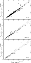 |
Fig. A.1. Comparison of effective radii as measured with this work procedures vs. van der Wel et al. (2014) estimates adopted for the field reference sample. Measurements are compared for a random portion of the control field galaxy sample (see text), split by Sersic index as indicated. The solid lines show the bisector (middle), and the expected average uncertainty (1σ) on effective radii from this work, as estimated with simulations (see Sect. 2.4) for sources at the faint end of the probed magnitude range. |
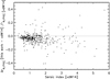 |
Fig. A.2. Comparison of effective radii as measured with this work procedures vs. van der Wel et al. (2014) estimates adopted for the field reference sample. For the same sources as in Fig. A.1, the fractional difference between the two measurements is shown as a function of Sersic index (two sources (< 1%) falling outside of the plotted range are not shown). |
In Fig. A.3, we similarly compare our Sersic index measurements versus van der Wel et al. (2014) for the same sources. We find a systematic offset towards lower values than those in van der Wel et al. (2014), by ∼4% for the overall population in the magnitude range of interest. At face value, the offset for sub-samples split by Sersic index is ∼4% and 7% for n < 1.5 and 1.5 < n < 2.5 sources, respectively, and consistent with no systematic offset for n > 2.5 sources, but possible variation with Sersic index is not significant with the given statistics. Indeed, Fig. A.3 clearly shows the dispersion between the two measurements, of order 15% for disk-dominated galaxies and 20−25% for intermediate and bulge-dominated systems. For reference, the expected average uncertainty on Sersic indices, as estimated from simulations (Sect. 2.4) for sources towards the faint end of our probed range, is ∼10%. Based on this comparison, with respect to the broad Sersic index classes considered in this work, and taking van der Wel et al. (2014) measurements as the reference for the purpose of this assessment, 6% of n < 1.5 sources would be misclassified as n > 1.5, out of which 2% with n > 2.5; at the same time, 20% of n > 2.5 sources would be misclassified as n < 2.5, out of which 2% as n < 1.5. As may be expected, misclassification may be more severe for intermediate Sersic sources, with almost 40% of 1.5 < n < 2.5 sources in van der Wel et al. (2014) being “misclassified” with our measurements, mostly (25%) as disky n < 1.5 systems.
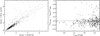 |
Fig. A.3. Comparison of Sersic indices as measured with this work procedures vs. van der Wel et al. (2014) estimates adopted for the field sample, for the same sources as in Fig. A.1 (see text). Left: The direct comparison of the two measurements. The solid lines show the bisector (middle), and the expected average uncertainty (1σ) on Sersic indices from this work, as estimated with simulations (see Sect. 2.4) for sources at the faint end of the probed magnitude range. Right: The fractional difference between the two measurements as a function of m160 magnitude (3% of the sources out of the plotted range are not shown). Symbols are coded by Sersic index, as in Fig. A.1. |
Given the intrinsically broad nature of morphology classes used in the analysis in Sect. 3, the impact of potential systematics at the level discussed here above on the results presented in this work turns out to be very marginal. Correcting Sersic indices of cluster galaxies by the amounts discussed above gives differences on the results and figures presented here that are always well within the quoted uncertainties, and are actually not noticeable in most cases. Therefore, as discussed in Sect. 3, Sersic indices presented throughout and all related results are shown with no corrections applied.
Appendix B: Additional measurements related to size difference of cluster versus field galaxies
Figure A.4 shows additional measurements related to the investigation of size differences between cluster and field galaxies for different sub-populations, as discussed in Sect. 3.2. In particular, Fig. A.4 shows 1) analogous measurements as in Fig. 5, but with average size differences as measured (not corrected for estimated size bias with respect to control field sample, see Sects. 2.4 and 3.2); 2) the impact of residual background contamination correction (see Sects. 2.2.1 and 3.2); 3) the lack of redshift dependence of average size measurements for the reference field sample (see discussion in Sect. 3.2).
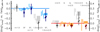 |
Fig. A.4. As Fig. 5, but showing sizes for cluster galaxies as measured (not corrected for estimated size bias with respect to control field sample, see text for details). Empty symbols also show the measurement for the full relevant candidate cluster member samples, not accounting for residual background contamination (solid symbols account instead for residual background contamination as in Fig. 5). The three vertical lines on the left of the control field measurements show the field sample split by redshift (1.3 < z < 1.5, 1.4 < z < 1.6, 1.6 < z < 1.8), showing no redshift dependence in the field measurements across the redshift range of interest. |
All Tables
All Figures
|
Fig. 1. Observed m814−m140 vs. m140−[3.6] colour-colour diagram of candidate cluster members at r/r500 < 0.7 for all clusters, down to the m140 limit indicated in each panel, coded by best-fit Sersic index as indicated in the legend (dark red, green and blue symbols). Filled and empty symbols show, respectively, galaxies above and below the stellar mass completeness limit for the individual cluster (Table 1). Symbol size scales with the statistical background-subtraction weight (Sect. 2.2.1; smaller symbols are overall more likely to be interlopers). In each panel, the black line marks the adopted separation between quiescent and star-forming galaxies, following S19. The background colour scale traces the median Sersic index (see legend) across the colour diagram (within a colour distance of 0.1 mag) of galaxies in the reference field sample with photo-zs within ±0.1 from the cluster’s redshift, and same m140 magnitude limit (only colour bins with at least five galaxies are shown). |
| In the text | |
|
Fig. 2. Morphology mix of massive galaxies in the probed cluster regions and in the reference field at 1.3 < z < 1.8. Left panel: fraction of log(M/M⊙) > 10.85 cluster galaxies with Sersic indices n ≤ 1.5, 1.5 < n < 2.5 and n ≥ 2.5 (dark grey symbols), and the corresponding fractions for the field reference sample (grey bars). For clarity, error bars (binomial, Cameron 2011) are only shown for cluster samples. Right panel: analogous fractions for the quiescent and star-forming populations, as indicated. Solid (empty) symbols refer to cluster galaxy samples excluding (including) sources within ±0.1 mag around the quiescent vs. star-forming classification border. Solid (hatched) bars analogously refer to the corresponding field reference samples. |
| In the text | |
|
Fig. 3. Distribution of axis ratios of log(M/M⊙) > 10.85 quiescent cluster galaxies in the probed cluster regions across the whole cluster sample (red shades) and in the reference field at 1.3 < z < 1.8 (blue shades, as indicated). For both cluster and field samples, darker (lighter) lines correspond to excluding (including) sources within ±0.1 mag around the quiescent vs. star-forming classification border. Error bars on the fractions over the whole population (binomial, Cameron 2011) are slightly offset for clarity. For comparison, the axis ratio distribution of star-forming field galaxies in the same mass and redshift range (grey line, errors within line width), and for 1 < z < 1.4 cluster galaxies in the same stellar mass range from Chan et al. (2021, hatched region, see text for details) are also shown. |
| In the text | |
|
Fig. 4. Stellar mass – size relation of candidate cluster members and field counterparts, split by Sersic index as indicated. All candidate members in the m140-limited samples across the five clusters are shown, with symbol size scaling with residual statistical background subtraction weights (Sect. 2.2.1). All sizes for both candidate members and field counterparts are scaled to a common redshift z = 1.5 for the purpose of this figure (see text). Candidate cluster members are shown with darker symbols, colour-coded by quiescent (red) vs. star-forming (blue) classification (purple and black symbols show, respectively, galaxies within ±0.1 mag from the classification border, and with no reliable classification). Large grey open squares indicate cluster BCGs (right hand panel). Light blue and light red squares in the background show counterparts from the control field sample at 1.35 < z < 1.75. The red and blue lines show the best-fit mass-size relations for quiescent and star-forming galaxies from van der Wel et al. (2014, also scaled to z = 1.5). Vertical grey lines mark the minimum and maximum stellar mass completeness limits across the five clusters. |
| In the text | |
|
Fig. 5. Median log size difference of log(M/M⊙) > 10.85 cluster galaxies (darker symbols with error bars, corrected for residual background subtraction, see text) and of field counterparts at 1.3 < z < 1.8 (shaded rectangles showing the 16th–84th percentile range, see text) with respect to the expected size from the van der Wel et al. (2014) star-forming (left panel) and quiescent (right panel) relations. Median differences are shown for different sub-samples based on Sersic index (symbols as in Fig. 4, or squares for no Sersic index selection) and star-forming (blue colour shades) vs. quiescent (red colour shades) classification (grey symbols show samples selected by Sersic index only, regardless of star-forming vs. quiescent classification; see text). |
| In the text | |
|
Fig. 6. Median log size difference between cluster and field galaxies as derived from Fig. 5, for different population sub-samples (see text). Symbols and colour coding follow Fig. 5. Error bars show statistical uncertainties (including statistical background subtraction). Light shaded rectangles show the maximum impact on the median difference from potential residual uncorrected systematics. Dark shaded rectangles show the combined error including both statistical and systematic uncertainties (see text). |
| In the text | |
|
Fig. A.1. Comparison of effective radii as measured with this work procedures vs. van der Wel et al. (2014) estimates adopted for the field reference sample. Measurements are compared for a random portion of the control field galaxy sample (see text), split by Sersic index as indicated. The solid lines show the bisector (middle), and the expected average uncertainty (1σ) on effective radii from this work, as estimated with simulations (see Sect. 2.4) for sources at the faint end of the probed magnitude range. |
| In the text | |
|
Fig. A.2. Comparison of effective radii as measured with this work procedures vs. van der Wel et al. (2014) estimates adopted for the field reference sample. For the same sources as in Fig. A.1, the fractional difference between the two measurements is shown as a function of Sersic index (two sources (< 1%) falling outside of the plotted range are not shown). |
| In the text | |
|
Fig. A.3. Comparison of Sersic indices as measured with this work procedures vs. van der Wel et al. (2014) estimates adopted for the field sample, for the same sources as in Fig. A.1 (see text). Left: The direct comparison of the two measurements. The solid lines show the bisector (middle), and the expected average uncertainty (1σ) on Sersic indices from this work, as estimated with simulations (see Sect. 2.4) for sources at the faint end of the probed magnitude range. Right: The fractional difference between the two measurements as a function of m160 magnitude (3% of the sources out of the plotted range are not shown). Symbols are coded by Sersic index, as in Fig. A.1. |
| In the text | |
|
Fig. A.4. As Fig. 5, but showing sizes for cluster galaxies as measured (not corrected for estimated size bias with respect to control field sample, see text for details). Empty symbols also show the measurement for the full relevant candidate cluster member samples, not accounting for residual background contamination (solid symbols account instead for residual background contamination as in Fig. 5). The three vertical lines on the left of the control field measurements show the field sample split by redshift (1.3 < z < 1.5, 1.4 < z < 1.6, 1.6 < z < 1.8), showing no redshift dependence in the field measurements across the redshift range of interest. |
| In the text | |
Current usage metrics show cumulative count of Article Views (full-text article views including HTML views, PDF and ePub downloads, according to the available data) and Abstracts Views on Vision4Press platform.
Data correspond to usage on the plateform after 2015. The current usage metrics is available 48-96 hours after online publication and is updated daily on week days.
Initial download of the metrics may take a while.