| Issue |
A&A
Volume 670, February 2023
|
|
|---|---|---|
| Article Number | A96 | |
| Number of page(s) | 10 | |
| Section | Extragalactic astronomy | |
| DOI | https://doi.org/10.1051/0004-6361/202245118 | |
| Published online | 10 February 2023 | |
X-ray analysis of JWST’s first galaxy cluster lens SMACS J0723.3−7327⋆
Max Planck Institute for Extraterrestrial Physics, Giessenbachstrasse 1, 85748 Garching, Germany
e-mail: This email address is being protected from spambots. You need JavaScript enabled to view it.
Received:
1
October
2022
Accepted:
28
November
2022
Abstract
Context. SMACS J0723.3−7327 is the first galaxy cluster lens observed by James Webb Space Telescope (JWST). Based on its early release observation data, several groups have reported the results on strong lensing analysis and mass distribution of this cluster. The new lens model dramatically improves upon previous results, thanks to JWST’s unprecedented sensitivity and angular resolution. However, limited by the angular coverage of the JWST data, the strong lensing models only cover the central region. Conducting an X-ray analysis on the hot intracluster medium (ICM) is necessary to obtain a more complete constraint on the mass distribution in this very massive cluster.
Aims. In this work, we perform a comprehensive X-ray analysis of J0723 with an aim to obtain accurate ICM hydrostatic mass measurements, using the X-ray data from Spectrum Roentgen Gamma (SRG)/eROSITA and Chandra X-ray observatories. By comparing the hydrostatic mass profile with the strong lensing model, we aim to provide the most reliable constraint on the distribution of mass up to R500.
Methods. Thanks to the eROSITA all-sky survey and Chandra, which provide high signal-to-noise ratio (S/N) and high angular resolution data, respectively, we were able to constrain the ICM gas density profile and temperature profile with good accuracy both in the core and to the outskirts. With the density and temperature profiles, we computed the hydrostatic mass profile, which was then projected along the line of sight to compare with the mass distribution obtained from the recent strong lensing analysis based on JWST data. We also deprojected the strong lensing mass distribution using the hydrostatic mass profile obtained in this work.
Results. The X-ray results obtained from eROSITA and Chandra are in very good agreement. The hydrostatic mass profiles we measured in this work, both projected and deprojected, are in good agreement with recent strong lensing results based on JWST data, at all radii. The projected hydrostatic mass within 128 kpc (the estimated Einstein radius) is (8.0 ± 0.7)×1013 M⊙, consistent with the strong lensing mass reported in recent literature. With the hydrostatic mass profile, we measured R2500 = 0.54 ± 0.04 Mpc and M2500 = (3.5 ± 0.8)×1014 M⊙, while the R500 and M500 are 1.32 ± 0.23 Mpc and (9.8 ± 5.1)×1014 M⊙, with a relatively larger error bar due to the rapidly decreasing S/N in the outskirts. We also find that the radial acceleration relation in J0723 is inconsistent with the RAR for spiral galaxies, implying that the latter is not a universal property of gravity across all mass scales.
Key words: galaxies: clusters: intracluster medium / galaxies: clusters: individual: SMACS J0723.3−7327 / X-rays: galaxies: clusters
The images in Fig. 1 are only available at the CDS via anonymous ftp to cdsarc.cds.unistra.fr (130.79.128.5) or via https://cdsarc.cds.unistra.fr/viz-bin/cat/J/A+A/670/A96
© The Authors 2023
 Open Access article, published by EDP Sciences, under the terms of the Creative Commons Attribution License (https://creativecommons.org/licenses/by/4.0), which permits unrestricted use, distribution, and reproduction in any medium, provided the original work is properly cited.
This article is published in open access under the Subscribe-to-Open model.
Open access funding provided by Max Planck Society.
1. Introduction
Mass and mass distribution parameters in massive galaxy clusters are crucial in studying the properties of dark matter halos and the evolution of the large-scale structures in the Universe. There are several independent ways to measure the mass distribution of clusters, such as strong or weak gravitational lensing effects from background sources (see, e.g., Kneib & Natarajan 2011; Umetsu 2020; Chiu et al. 2022; Caminha et al. 2017; Bergamini et al. 2023), velocity dispersion of member galaxies (e.g., Girardi et al. 1993), hydrostatic equilibrium of the X-ray emitting intracluster medium (ICM; e.g., Ettori et al. 2013, 2019; Ghirardini et al. 2018), and CMB lensing (Melin & Bartlett 2015). Among these properties, the X-ray hydrostatic mass has the unique advantage of acquiring the deprojected mass distribution, while the other methods can only measure the line-of-sight (LoS) integrated mass. Another difference in these methods is that they are sensitive in different radial ranges. For example, strong lensing has the most prominent effect near the critical line (close to the core region, usually smaller than 0.3R500), where ICM hydrostatic mass may suffer from bias due to non-gravitational effects such as radiative cooling and AGN feedback particularly when a strong cool core exists and non-thermal pressure due to gas turbulence or bulk motions. Therefore, it is important to have the mass distribution in galaxy clusters measured from multiple independent methods to understand the biases in each of them.
In this work, we focus on a specific target, SMACS J0723.3−7327 (hereafter, J0723), a massive galaxy cluster at a redshift of 0.39 (Ebeling et al. 2001). J0723 (RA = 7:23:19.20, Dec = −73:27:22.5) was identified as a galaxy cluster in the southern extension of the Massive Cluster Survey (MACS; Ebeling et al. 2001). It was also detected in X-ray band in the ROSAT All-Sky Survey (RASS; Voges et al. 1999) and in Sunyaev-Zeldovich survey by Planck (Planck Collaboration XXIX 2014; Planck Collaboration XXVII 2016). J0723 is the first galaxy cluster lens observed by the James Webb Space Telescope (JWST). Based on the Early Release Observation data from JWST, several groups have reported their results from strong lensing analyses and the mass distribution of this cluster (Mahler et al. 2022; Caminha et al. 2022). The new lens model dramatically improves upon previous results, thanks to the unprecedented sensitivity and angular resolution of JWST, which have led to the discovery of significantly more multiple images and lensed sources. However, the JWST observation only covers the core of the cluster, which limits the strong lensing analysis to the central ∼200 kpc (Caminha et al. 2022), despite that Mahler et al. (2022) extrapolated the model to ∼1 Mpc. Since the strong lensing effect is only sensitive to the projected mass, the small coverage of the strong lensing model implies that, with the strong lensing results only, the mass distribution in cluster outskirts is unknown; hence, we cannot get the true and deprojected mass distribution in cluster center. Therefore, to obtain a more complete constraint on the mass distribution in J0723, the strong lensing model needs to be combined with other probes such as ICM hydrostatic analysis, which provides constraints on the mass distribution from the center to the outskirts.
J0723 has been observed in the X-ray band by Chandra and XMM-Newton. Using the archival data of XMM-Newton, Lovisari et al. (2020) measured the hydrostatic mass of J0723, but with only three bins in the temperature profile. Their results show that J0723 is massive ( ) and hot (
 keV). J0723 is also observed by eROSITA during its survey observation phase. In this work, we will perform an X-ray study on J0723 based on the eROSITA all-sky survey data, aimed at providing the projected and deprojected hydrostatic mass profiles, to the largest extent allowed by the data. Due to the relatively low angular resolution of eROSITA (FOV averaged half energy width HEW∼30″–35″ over the soft band), we also leverage the high angular resolution of the archival Chandra data to constrain the temperature profile in cluster center. On the other hand, the archival Chandra data is too shallow to constrain gas properties in cluster outskirts (see Fig. 1). The eROSITA all-sky survey data, thanks to its large effective area in soft energies, is most sensitive to low temperature gas at cluster outskirts (∼1400 cm2 at 1 keV). Therefore, it will play a crucial role to determine the gas density and temperature profiles up to ∼R500, which are key data in the conversion between projected and deprojected mass profiles. The results in this work will also be helpful to further verify the performance of eROSITA, improving our understanding of the calibration systematics in the analysis of eROSITA survey-mode data on very hot clusters (∼10 keV for J0723).
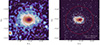 |
Fig. 1. X-ray image of J0723. Left panel: eROSITA exposure-corrected image in the 0.2–2.3 keV band, smoothed with a Gaussian of σ = 10″. Right panel: Chandra exposure-corrected image in the 0.5–7 keV band, smoothed with a Gaussian of σ = 2″. The images are centered at the coordinate (RA = 7:23:19.20, Dec = −73:27:22.5). The large and small red circles show the positions of R500 = 1.32 Mpc and R2500 = 0.54 Mpc, determined from the hydrostatic mass profile (R500/R2500 is the radius within which the average density is 500/2500 times the critical density at cluster’s redshift, see Sect. 3). On the eROSITA image, the emission of the cluster clearly extends to ∼R500. On the Chandra image, the emission only slightly exceeds R2500, but the cluster core is better resolved. The red point sources on the Chandra image (visible as larger white sources on the eROSITA image due to the larger PSF) are AGN which are masked in the analysis. Some bright point sources are marked on the eROSITA image. |
The paper is organized as follows. In Sect. 2, we introduce the eROSITA and Chandra X-ray datasets we used in this work and the reduction of these data. In Sect. 3, we present the X-ray data analysis, including the spectral and image fitting, and the computation of the mass profile. In Sect. 4, we discuss our results and possible caveats in our analysis. Our conclusions are summarized in Sect. 5. Throughout this paper, we adopt the concordance ΛCDM cosmology with ΩΛ = 0.7, Ωm = 0.3, and H0 = 70 km s−1 Mpc−1. At a redshift of z = 0.39, 1 arcsec corresponds to 5.29 kpc. The solar abundance table from Asplund et al. (2009) is adopted. X-ray spectral fitting in this work is done with Xspec version 12.11.1 (Arnaud 1996) using C-statistics (Cash 1979; Baker & Cousins 1984; Kaastra 2017). Quoted error bars correspond to a 1σ confidence level, unless noted otherwise.
2. X-ray data reduction
In this work, we used the X-ray data from eROSITA and Chandra. The eROSITA data are obtained during the all-sky survey (eRASS) from December 2019 to February 2022. J0723 was scanned five times in the first five all-sky surveys (eRASS:5). The total effective exposure after correcting for vignetting effect is ∼4.4 ks. We note that the exposure on J0723 is significantly larger than the average depth of eRASS, because it lies close to the south ecliptic pole of the survey. The Chandra observation (ObsID: 15296, PI: S. Murray) was performed in April 2014, with a cleaned exposure time of 16.5 ks.
2.1. eROSITA
The eRASS:5 data were processed with the eROSITA Science Analysis Software System (eSASS; Brunner et al. 2022)1. For all the seven telescope modules (TMs), we applied pattern recognition and energy calibration to produce calibrated event lists. In comparison with the data processing c001 from the eROSITA Early Data Release2, the data processing we performed in this work has an improved level of low-energy detector noise suppression, along with a better computation method for the subpixel position. The event lists are further filtered after the determination of good time intervals, dead times, corrupted events and frames, and bad pixels. Using star-tracker and gyro data, celestial coordinates were assigned to the reconstructed X-ray photons, which can then be projected into the sky to produce images and exposure maps. All valid pixel patterns are selected in this work, that is, single, double, triple, and quadruple events. The vignetting and point spread function (PSF) calibrations are less accurate in the corners of CCDs, therefore, we used only those photons that are detected at off-axis angles ≤30 arcmin. The soft band of TMs 5 and 7 are affected by light leaks (Predehl et al. 2021); therefore, we ignored the events below 1 keV of TMs 5 and 7 in our analysis. Point sources are detected in the eROSITA soft band (0.2–2.3 keV) image using the same method described in Brunner et al. (2022) and are masked from the analysis. We also include the point source list as detected by Chandra. The radius of the masked point source has the minimum value of 30″. For several bright point sources, the radius was increased manually to mask the residual emission due to the outer wings of the PSF. We checked the masked regions visually and confirmed that after masking, the residual contamination from point sources is negligible.
2.2. Chandra
The reduction of Chandra data was performed using the software CIAO v4.14, with the latest release of the Chandra Calibration Database at the time of writing (CALDB v4.9). Time intervals with a high background level were filtered out by performing a 2σ clipping of the light curve in the 2.3–7.3 keV band source-free image. The total cleaned exposure time after deflare is ∼16.5 ks.
Point sources within the field of view (FOV) were identified with wavdetect on the Chandra 0.5–7 keV band image, checked visually, and eventually masked. Gaps between the CCD chips are also masked. The eROSITA and Chandra images of J0723 are shown in Fig. 1. We note that while the ICM emission in cluster outskirts can be well detected by the eROSITA data, it is beyond the flux limit of the Chandra data, despite the fact that the Chandra data is also expected to play an important role in constraining the ICM properties in the core. Therefore, in the following analysis, we consider the Chandra results in the outskirts (> ∼600 kpc) as an extrapolation and we rely on the eROSITA measurements in these regions.
3. X-ray data analysis
In this section, we introduce our X-ray analysis for both eROSITA and Chandra. We performed a spectral analysis to measure the gas temperature profile, followed by an imaging analysis to measure the gas density. The mass profile was then derived from the temperature and density profiles using the hydrostatic equilibrium equation.
3.1. Spectral analysis
3.1.1. eROSITA
For the spectral analysis of eROSITA, we chose six annuli with outer radii of: 30″, 60″, 100″, 150″, 200″, and 270″. The center of the regions is RA = 7:23:19.20, Dec = −73:27:22.5, determined by fitting the Chandra image (see Sect. 3.2 and Fig. 1). The spectral extraction and the computing of ancillary response files (ARFs), and redistribution matrix files (RMFs) from the seven telescope modules are performed using the eSASS algorithm srctool. The background spectrum is extracted from a concentric annulus with inner and outer radii of 3.5 Mpc and 5 Mpc, far beyond the emission of the ICM. Fitting of the background spectrum is done using the similar approach described in Liu et al. (2022). The instrumental background due to the interactions of high-energy particles with the telescope and the satellite is obtained by fitting the filter-wheel-closed (FWC) data with a broken power-law and a series of Gaussian lines (Freyberg et al. 2020). We used the best-fitting parameters obtained from the FWC data to fit the local background, but allowing a free overall normalisation. The cosmic X-ray background (CXB) is modeled by considering the contribution from the Local Hot Bubble (e.g., Snowden et al. 2008; Kuntz & Snowden 2000), the Galactic Halo, and unresolved point sources. The Local Hot Bubble and the Galactic Halo are modeled by an unabsorbed and absorbed apec (Smith et al. 2001; Foster et al. 2012), while the emission due to unresolved sources is modeled by an absorbed powerlaw, where the index is frozen to 1.46 (see, e.g., Luo et al. 2017). The Galactic hydrogen absorption is modeled using tbabs (Wilms et al. 2000), where the hydrogen column density nH is fixed to 22.5 × 1020 cm−2, according to the nH, tot value provided by Willingale et al. (2013). Therefore, our final CXB model is: apec+tbabs(apec+powerlaw). The ICM emission is modeled with a single apec model, where the redshift is fixed at 0.39, metal abundance is fixed at 0.3. We do not make any attempt to measure the chemical property of the ICM in this work, as the metallicity of massive clusters is very well constrained from the cluster center (e.g., Liu et al. 2018, 2020) to the outskirts (e.g., Mernier et al. 2018; Ezer et al. 2017; Bulbul et al. 2016; Simionescu et al. 2017), while the line emission is negligible in such a hot cluster as J0723.
A common issue in a combined analysis of clusters using the data from multiple telescopes is the discrepancy in the temperatures measured by different instruments. For example, Schellenberger et al. (2015) found that the cluster temperatures measured by XMM-Newton/EPIC are significantly lower than those reported by Chandra/ACIS. They also found that the difference is mostly due to the discrepancy in the cross-calibration in the soft band and that the temperatures measured only using the hard band are more consistent.
Therefore, in the eROSITA analysis, we adopted the temperatures constrained from the hard band spectra (2–8 keV). Given the low number of counts we have for J0723, we were not able to perform hard-band fitting for all the bins in the temperature profile. However, this bias is systematic, and we can simply get a conversion factor: fT ≡ ln Thard/ln Tfull, from a high S/N spectrum, and we applied this conversion to the Tfull of the spectrum with lower S/N, where Thard cannot be constrained. To obtain the conversion factor fT, we extracted the spectrum within 2 arcmin to make sure the spectrum has a high S/N, and we fit the full band (0.5–8 keV) and hard band (2–8 keV) spectra, respectively. The best-fit temperatures are  keV and
  keV. Therefore, we have fT = 1.417. It should be noted that since we assume a systematic conversion between Thard and Tfull, we ignore the statistical uncertainties of Thard and Tfull in the computation of fT, but only use the best-fit values. As a comparison, we also measured the temperature with Chandra for the same region and the result is
  keV, which is in very good agreement with the eROSITA hard band result. In Table 1, we list the temperature values in each bin by fitting the full band, along with the modified values, using the above strategy.
Temperature profile measured by eROSITA before and after the hard-band modification.
The modified temperature profile we obtained from the eROSITA data is plotted in Fig. 2. We note that the two innermost bins only have widths of 30″, thus the spectra are unavoidably affected by PSF spilling of the adjacent bin. However, this effect should be no more than a slight smoothing of the profile. We stress that in these regions we have Chandra data with better resolution, thus the contribution of the eROSITA temperature profile is more significant in the outskirts. Therefore, the impact of PSF spilling can be safely ignored in these regions.
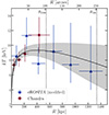 |
Fig. 2. Temperature profile of J0723. Blue and red data points are from the analysis of eROSITA (after modification using hard-band results) and Chandra, respectively. The solid black curve and shaded area are the best-fit model of the profile. The two dotted lines indicate the positions of R500 = 1.32 Mpc and R2500 = 0.54 Mpc, determined from the hydrostatic mass profile measured by eROSITA (blue line in Fig. 5, see Sect. 3.3, same for the other figures). |
3.1.2. Chandra
For the spectral analysis of the Chandra data, we increased the spatial resolution of the temperature profile in the central region (R < 50″) with respect to the eROSITA result. The ARF and RMF of each spectrum were computed with the commands mkarf and mkacisrmf. The background spectra were extracted from the ‘blank sky’ files, and processed using the blanksky script (we used the default options with weight_method ‘particle’ and bkgparams = [energy = 9000:12000]). We used the full energy range (0.5–7 keV) for the fit. We also carried out the same analysis based only on the hard band (2–7 keV), as we had done for eROSITA. However, we find no significant difference between the Thard and Tfull for Chandra. This is probably because of the much smaller effective area of Chandra in the soft band, which does not contribute much to the fit. We, therefore, adopted the full band fitting results for Chandra. The temperature profile from Chandra data is plotted in Fig. 2.
Using Chandra data, we also performed a spatially resolved spectral analysis to measure the 2D distribution of temperature to search for any peculiar structure and inspect the consistency with the 1D profile. The regions for the 2D analysis were selected using the Voronoi tessellations method (Cappellari & Copin 2003). Each region contains ∼300 net counts in the energy range 0.5–7 keV. The temperature map and its uncertainty are shown in Fig. 3. We find that the 1D temperature file is in broad consistent with the 2D map. A clear cool core at ∼7 keV can be observed in the temperature map, in accordance with the temperature profile.
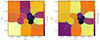 |
Fig. 3. ICM temperature distribution measured with Chandra data. Left and right panels show the maps of temperature and 1σ uncertainty, respectively. The contours colored in cyan are generated from the 0.5–7 keV Chandra image. |
3.1.3. Combined temperature profile
In general, the results of eROSITA and Chandra are in good agreement, particularly in the central regions. In the outskirts, both datasets have large error bars. J0723 hosts a weak cool core, with Tcore ∼ 7 keV and Tmax ∼ 10 keV. Considering that the temperature variance within our datasets is less than a factor of 2, the difference between projected and deprojected temperature profiles is expected to be rather small, well below the statistical uncertainty. Therefore, we do not make any attempt to deproject the temperature profile.
The eROSITA and Chandra combined temperature profile was fit with the model presented in Vikhlinin et al. (2006) to get a smooth temperature profile:
![Mathematical equation: $$ \begin{aligned} T(r)=T_0 \cdot \frac{(r/r_{\rm cool})^{a_{\rm cool}}+T_{\rm min}/T_0}{(r/r_{\rm cool})^{a_{\rm cool}}+1} \cdot \frac{(r/r_{\rm t})^{-a}}{[1+(r/r_{\rm t})^b]^{c/b}}. \end{aligned} $$](/articles/aa/full_html/2023/02/aa45118-22/aa45118-22-eq18.gif) (1)
(1)
The fitting was done using the MCMC tool of Foreman-Mackey et al. (2013). The best-fit profile is shown in Fig. 2. The best-fit parameters of the model are listed in Table 2.
Best-fit parameters and uncertainties for the temperature profile.
3.2. Image fitting with MBProj2D
To measure the gas density profile, we performed an imaging analysis using the MultiBand Projector 2D (MBProj2D) tool3. This (Sanders et al. 2018) is a code that forward models background-included X-ray images of galaxy clusters to fit cluster and background emission simultaneously, while measuring the profiles of ICM properties including density, flux, luminosity, and so on. By using a single band image, MBProj2D is only sensitive to the density of the ICM. By using multiple bands from soft to hard and given enough counts, MBProj2D is also able to model the temperature variation within the cluster. When sufficient energy bands are provided, MBProj2D can give equivalent results as expected from spatially-resolved spectral analysis; for instance, the metallicity and temperature profiles of the ICM. By assuming hydrostatic equilibrium, MBProj2D can also measure the hydrostatic mass profile. We refer to Sanders et al. (2018) for more details on MBProj2D4.
In this work, since we already have access to the temperature profile from the spectral analysis, we only needed to use the basic function of MBProj2D to measure the density profile using multiple band images, without assuming a hydrostatic mass model. We then derived the model-independent hydrostatic mass profile backwardly using the temperature and density profiles. For the eROSITA data, we create images and exposure maps in the following energy bands (in units of keV): [0.3–0.6], [0.6–1.0], [1.0–1.6], [1.6–2.2], [2.2–3.5], [3.5–5.0], [5.0–7.0], using the evtool command in eSASS. The size of the image is 6 Mpc × 6 Mpc, which is large enough to include the background. Point sources within the image are masked following the same approach in the spectral analysis. The PSF and ARF variations across different bands are considered properly. The model of density profile is from Vikhlinin et al. (2006), but without the second β component:
 (2)
(2)
where ne and np are electron density and proton density, and we assume ne = 1.21np. γ is fixed at 3. n0, rc, α, β, rs, and ϵ are free parameters.
A similar analysis was done also for the Chandra data. The following energy bands (in units of keV) are used for Chandra analysis: [0.5–0.75], [0.75–1.0], [1.0–1.25], [1.25–1.5], [1.5–2.0], [2.0–3.0], [3.0–4.0], [4.0–5.0], [5.0–6.0], [6.0–7.0]. Limited by the FOV of Chandra, the size of the image is reduced to 4 Mpc × 4 Mpc. However, this is still large enough to contain the background emission in the fitting. The Chandra exposure map computed by CIAO is always folded by the effective area. In order to get the unfolded exposure map as required by MBProj2D, we extracted a spectrum in the center of the image and renormalised the folded exposure maps using the exposure time information of the spectrum.
The electron density profiles measured using MBProj2D are plotted in Fig. 4. The best-fit parameters are provided in Table 3. In Fig. 4, we also show the cumulative gas mass profiles. The results from eROSITA and Chandra are in very good agreement. There is only a very small discrepancy in the density profile in the outskirts, which is acceptable considering that the Chandra data is too shallow in these regions, thus the Chandra result is probably an extrapolation of the best-fit model dominated by the central region.
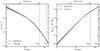 |
Fig. 4. Results of X-ray imaging analysis from eROSITA and Chandra using MBProj2D. Left and right panels show the electron density profiles and gas mass profiles, respectively. The Chandra results above 0.6 Mpc are plotted as dashed lines. |
Best-fit parameters and uncertainties for electron density profiles.
3.3. Hydrostatic mass
With the ICM temperature profile and density profile, we can derive the hydrostatic mass profile using the hydrostatic equilibrium equation:
 (3)
(3)
where kB is the Boltzmann constant, G is the gravitational constant, μ = 0.6 is the mean atom weight, and mp is proton mass; ρg = nempA/Z is the gas density, where A ∼ 1.4 and Z ∼ 1.2 are the average nuclear charge and mass for ICM with 0.3 solar abundance. The uncertainty on the mass profile was computed by randomly picking 2000 samples in the Markov chains of the temperature and density profiles.
The hydrostatic mass profiles measured by eROSITA and Chandra are plotted in the left panel of Fig. 5. We note that since we are using the combined temperature profile, the difference in the two profiles results only from the density profiles. We find that the results obtained from eROSITA and Chandra are in very good agreement, despite the small discrepancies in the very center (< 50 kpc) and the outskirts (> 1 Mpc), which are well within the limits of the error bar. From the mass profile measured by eROSITA (see the blue line in Fig. 5), we obtained R2500 = 0.54 ± 0.04 Mpc and R500 = 1.32 ± 0.23 Mpc, along with the masses within the two radii M2500 = (3.5 ± 0.8)×1014 M⊙ and M500 = (9.8 ± 5.1)×1014 M⊙. The values computed from the Chandra results are fully consistent (see Table. 4). The error bars in R500 and M500 are large, due to the relatively larger uncertainty of the temperature in the outskirts. We also found an ideal agreement with the published results of Lovisari et al. (2020), who measured  using the archival data of XMM-Newton. The temperature measured by Lovisari et al. (2020),
  keV, is slightly lower compared to our temperature profile, but still consistent within 1σ. We also compared the mass of J0723 we measured in this work to the published L − M scaling relation of galaxy clusters. From the luminosity profile measured with MBProj2D using eROSITA data, we obtained
  erg s−1 in the 0.5–2 keV band. Adopting the L − M scaling relation for high redshift and massive clusters in Bulbul et al. (2019), the corresponding mass is
  , which is in very good agreement with our results.
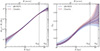 |
Fig. 5. Results of hydrostatic analysis. Left panel: hydrostatic mass profiles of J0723 using the best-fit model of the combined temperature profile (Fig. 2) and the density profile of eROSITA (blue) and Chandra (red). Right panel: gas mass fraction (fgas) profiles. The two dotted lines indicate the positions of R500 = 1.32 Mpc and R2500 = 0.54 Mpc, determined from the hydrostatic mass profile measured by eROSITA (blue line in the left panel). |
Comparison between eROSITA and Chandra in the measurements of cluster masses within R500 and R2500.
With the hydrostatic mass and gas mass profiles, we also computed the profile of gas mass fraction (fgas), shown in the right panel of Fig. 5. With the eROSITA data, we measured  and
and  . From the profile, we can observe a clear trend that fgas decreases from > 10% in the outskirts (> 1 Mpc) to < 5% in the core (< 50 kpc), despite the fact that the former has high uncertainty. This is consistent with the picture that describes how in massive galaxy clusters, the dark matter halo and stellar mass are more concentrated than the hot gas, thus the former dominate the total mass in the center, while the mass budget tends to be more consistent with the average of the Universe when extending to larger radii (see, e.g., Eckert et al. 2013; Planck Collaboration XII 2016).
In order to make a comparison with the strong lensing results, we computed the LoS projected mass using our hydrostatic mass profiles. The projected mass profiles are shown in Fig. 6. We compared our results with the recent strong lensing results published in Caminha et al. (2022), who measure the cluster mass distribution with 46 multiple images from 16 background sources. We find remarkable consistency between the eROSITA hydrostatic mass and the strong lensing mass at all radii. At the estimated Einstein radius 128 kpc (Caminha et al. 2022), eROSITA measured a projected hydrostatic mass of (8.0 ± 0.7)×1013 M⊙, which is in good agreement with the result reported in Caminha et al. (2022): (8.6 ± 0.2)×1013 M⊙. The measurement of Chandra at the same radius: (7.6 ± 0.7)×1013 M⊙, is only slightly (∼1σ) lower than the strong lensing result, while these values tend to be more consistent at larger radii. Using the same JWST data, another team measured a strong lensing mass of (7.6 ± 0.2)×1013 M⊙ at 128 kpc (Mahler et al. 2022), which contradicts the result of Caminha et al. (2022) at ∼4σ. On the other hand, we note that the result of Mahler et al. (2022) is consistent with our results for both eROSITA and Chandra within 1σ.
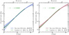 |
Fig. 6. LoS projected mass profiles of J0723 measured by eROSITA (left panel) and Chandra (right panel). The green curve shows the mass distribution from strong lensing analysis with multiple images discovered by JWST (see Fig. A.1 of Caminha et al. 2022). The green bars shows the positions of the multiple images used in the strong lensing analysis. |
As a further check, we also deprojected the strong lensing mass profile from Caminha et al. (2022) using the hydrostatic mass profiles measured by eROSITA and Chandra, respectively, and compared it with the hydrostatic mass profiles. From the comparison shown in Fig. 7, the consistency between eROSITA and strong lensing results still remains good. For Chandra, the two profiles are also consistent within ∼1σ.
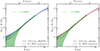 |
Fig. 7. Comparison between the hydrostatic (hydro) mass profile (blue and red curves) and the strong lensing (SL) mass profile in Caminha et al. (2022) after deprojection (green curves). Left panel is for eROSITA and right panel is for Chandra. |
We also remark that there are many other strong lensing analyzes published in literature, both before and after JWST, thanks to the rapid development of lensing modelization techniques and optical spectroscopic surveys in recent years (e.g., Fox et al. 2022; Golubchik et al. 2022; Sharon et al. 2023). Despite the fact that most of these works provide consistent results in the center (< 200 kpc), there are tensions at larger radii due to the different tools and data they used. However, here we refrain from comparing our results with all the available strong lensing results and from discussing the tensions between them, which are beyond the goal of this work.
4. Discussion
In this section, we discuss the systematics and caveats in our analysis. A possible source of bias to our results is the deviation from hydrostatic equilibrium of the ICM in J0723. This so-called “hydrostatic mass bias” can be caused by major and minor mergers (e.g., Markevitch et al. 2002; Vikhlinin et al. 2001), core sloshing (e.g., Markevitch et al. 2001; Sanders et al. 2005), gas turbulence (only a few percent, see Eckert et al. 2019), possible global rotation (Liu & Tozzi 2019), and other non-gravitational processes such as AGN feedback (Fabian 2012). On the Chandra image, there are no signs of violent mergers. Weak emission excess is visible ∼400 kpc to the northeast of the X-ray peak (see the right panel of Fig. 1) that is possibly associated with a gas clump; however, it is too close to the cluster center and too faint, thus it only has a negligible impact on the hydrostatic analysis. The offset between the X-ray peak and the position of the brightest cluster galaxy (BCG) is ∼6″, corresponding to ∼30 kpc, or ∼0.02R500, which implies that J0723 is in a relaxed dynamical state (see, e.g., Rossetti et al. 2016; Seppi et al. 2021). Moreover, with a visual inspection on the Chandra image, we do not find any significant structure related with AGN mechanical feedback, such as cavities. Although such a visual inspection is limited by the number of photons and it is hard to quantify either the existence or non-existence of cavities, we can conservatively conclude that the impact of feedback is not strong enough to affect our results.
On the Chandra image, there is also a mild signal of asymmetry in the central region, which may indicate the sloshing of the core. On the temperature map (see Fig. 3), the coolest region seems to be closer to the west edge of the core, instead of the X-ray peak, which indicates a possible sloshing of the cool core that is consistent with the surface brightness image. However, limited by the data quality, we were not able to make further analysis on the dynamical status of the core. In any case, we can confirm that J0723 is aptly virialized, and the impact of non-hydrostatic gas on the measurement of the hydrostatic mass can be ignored. Most studies so far have suggested a hydrostatic mass bias of a few to ∼20%, from the most relaxed clusters to the extremely disturbed ones (see Pratt et al. 2019, for a review). The bias is sensitive to the dynamic status of the cluster, and the radius within which the masses are measured. For J0723, the hydrostatic masses we measured are within 1σ with the strong lensing masses which are only available in the central region. In the outskirts (∼R500), the uncertainty in the hydrostatic mass profile increases to > 50%, far beyond the typical value of hydrostatic bias for relaxed clusters, and the strong lensing measurements are not available. Therefore, with the results in this work, we do not observe a statistically significant hydrostatic bias.
With the gas mass and hydrostatic mass profiles, we also made an attempt to study the radial acceleration relation (RAR) in J0723. This relation describes the relation between the centripetal accelerations due to the total mass (gtot = GMtot/r2) and baryonic mass (gbar = GMbar/r2 = G(Mgas + M*)/r2) without introducing dark matter. Studying RAR in gravitationally bound systems is useful to verify modified gravity theories, such as modified Newtonian dynamics (MOND, Milgrom 1983). A universal RAR across all mass scales is regarded as an important support for MOND. So far, a tight and universal RAR has been achieved in a number of studies on galaxies (McGaugh et al. 2016; Lelli et al. 2017; Li et al. 2018; Brouwer et al. 2021). For example, McGaugh et al. (2016) found that the RAR of 153 spiral galaxies fits well with the following model:
 (4)
(4)
where g† = 1.20 ± 0.02 (random) ±0.24 (systematic) ×10−10 m s−2.
On the other hand, the RAR in galaxy clusters is less clear. Not only is the normalization of acceleration higher than what is found for galaxies (e.g., Tian et al. 2020), but also the overall shape of the observed cluster RAR clearly deviates from the model in Eq. (4), implying a completely different RAR between clusters and galaxies (e.g., Eckert et al. 2022; Tam et al. 2022).
To compute the RAR in J0723, we use the hydrostatic mass profile and gas mass profile obtained from eROSITA. Baryonic mass in the central region is dominated by stars in the BCG and intracluster light (ICL), where we do not have constraint on the stellar mass profile. We thus ignore the core with a size of 200 kpc in the following discussion. Beyond the core, the contribution of stellar mass in the total mass budget is roughly a constant at ∼2% up to 2.5 Mpc (see, e.g., Andreon 2015; Eckert et al. 2022). Therefore, we approximate the stellar mass profile M*(r) as 0.02 × Mtot(r), adding on a systematic uncertainty of 50%. Since stellar mass only contributes 10%–15% in baryonic mass at large radii (Eckert et al. 2022), this rough estimation will not significantly affect our results.
The RAR in J0723 is shown in Fig. 8. Depite the large errorbar and the narrow range in gbar and gtot, we clearly observe that the J0723 RAR is inconsistent with the model of McGaugh et al. (2016) for spiral galaxies. The discrepancy is so large that it cannot be explained by either the possible biases or systematics in our analysis, such as the uncertainty in stellar mass and hydrostatic bias, or the 0.12 dex scatter in the McGaugh et al. (2016) relation. This is in broad agreement with the results for X-COP clusters (Eckert et al. 2022) and BAHAMAS simulation (Tam et al. 2022). Due to the removal of the core, we have no constraints on gbar at high acceleration, where Eckert et al. (2022) observed that the RAR of X-COP clusters eventually catched up with the McGaugh et al. (2016) relation for galaxies. However, this trend is largely predictable as the core region with high acceleration is dominated by the BCG, while ICM only constitutes a small fraction in the total baryonic mass. In summary, we find that the RAR found in galaxies cannot fit the data of the cluster J0723, thus our results do not support a universal RAR across all mass scales.
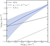 |
Fig. 8. Radial acceleration relation of J0723. The dashed line shows the RAR in spiral galaxies obtained by McGaugh et al. (2016). The dotted line indicates the Y = X relation. |
5. Conclusions
In this work, we performed an X-ray analysis on the galaxy cluster SMACS J0723.3−7327, using the all-sky survey data from the SRG/eROSITA telescope and Chandra observatory. The azimuthally averaged profiles of ICM temperature and density were measured with high accuracy from cluster center to the outskirts (∼R500), from which the hydrostatic mass profile is derived. While the high-angular-resolution Chandra data sees most of its contribution in the measurement of the temperature profile in the center, the eROSITA data dominates the constraints from the center to the outskirts, thanks to the significantly larger effective area (effective area ratio between eROSITA and Chandra in 2014 is ∼10 in the 0.5–2 keV band and ∼2 in the 2–7 keV band). Both eROSITA and Chandra are consistent with each other in the measurements of temperature, density, gas mass, and hydrostatic mass, particularly within ∼R2500, while the Chandra results in the outskirts are less conclusive due to the shallow observation. The X-ray results are compared with the lens mass model constrained from strong lensing analysis with the latest JWST data (Caminha et al. 2022). We find a remarkable consistency between the X-ray hydrostatic mass profile and the strong lensing mass distribution at all radii (the latter ends at ∼400 kpc), both projected and deprojected. We also find that the radial acceleration relation (RAR) in J0723 is inconsistent with the RAR for spiral galaxies, implying that the latter is not a universal property of gravity across all mass scales.
With the published results of the Early Data Release, eROSITA has proved its capability, particularly in the detection and study of low-mass clusters and groups (see, e.g., Liu et al. 2022; Bulbul et al. 2022; Klein et al. 2022; Bahar et al. 2022; Ghirardini et al. 2022; Pasini et al. 2022; Veronica et al. 2022). In this study, we focus on J0723, a more massive cluster at a high redshift (z = 0.39) and with a high temperature (∼10 keV). With the eRASS:5 survey depth data, we measured the X-ray properties of the cluster with comparable accuracy to that reached in the same analysis using deeper Chandra data. A similarly hot cluster, A3266, was studied as a calibration target in Sanders et al. (2022), but it is located at a much lower redshift and with a deeper pointing observation. Therefore, with this work, we further verify the capability of eROSITA, as well as the potential of the all-sky survey data, in the study of massive and distant galaxy clusters.
Version eSASSusers_211214_0_4.
Acknowledgments
We thank the anonymous referee for his/her constructive comments that helped improve the paper. We thank G. B. Caminha for providing the JWST strong lensing model. This work is based on data from eROSITA, the soft X-ray instrument aboard SRG, a joint Russian-German science mission supported by the Russian Space Agency (Roskosmos), in the interests of the Russian Academy of Sciences represented by its Space Research Institute (IKI), and the Deutsches Zentrum für Luft- und Raumfahrt (DLR). The SRG spacecraft was built by Lavochkin Association (NPOL) and its subcontractors, and is operated by NPOL with support from the Max Planck Institute for Extraterrestrial Physics (MPE). The development and construction of the eROSITA X-ray instrument was led by MPE, with contributions from the Dr. Karl Remeis Observatory Bamberg and ECAP (FAU Erlangen-Nuernberg), the University of Hamburg Observatory, the Leibniz Institute for Astrophysics Potsdam (AIP), and the Institute for Astronomy and Astrophysics of the University of Tübingen, with the support of DLR and the Max Planck Society. The Argelander Institute for Astronomy of the University of Bonn and the Ludwig Maximilians Universität Munich also participated in the science preparation for eROSITA. The eROSITA data shown here were processed using the eSASS/NRTA software system developed by the German eROSITA consortium. A.L. and E.B. acknowledge financial support from the European Research Council (ERC) Consolidator Grant under the European Union’s Horizon 2020 research and innovation programme (grant agreement CoG DarkQuest No 101002585).
References
- Andreon, S. 2015, A&A, 575, A108 [NASA ADS] [CrossRef] [EDP Sciences] [Google Scholar]
- Arnaud, K. A. 1996, ASP Conf. Ser., 101, 17 [Google Scholar]
- Asplund, M., Grevesse, N., Sauval, A. J., & Scott, P. 2009, ARA&A, 47, 481 [NASA ADS] [CrossRef] [Google Scholar]
- Bahar, Y. E., Bulbul, E., Clerc, N., et al. 2022, A&A, 661, A7 [NASA ADS] [CrossRef] [EDP Sciences] [Google Scholar]
- Baker, S., & Cousins, R. D. 1984, Nucl. Instrum. Methods Phys. Res., 221, 437 [Google Scholar]
- Bergamini, P., Acebron, A., Grillo, C., et al. 2023, A&A, 670, A60 [NASA ADS] [CrossRef] [EDP Sciences] [Google Scholar]
- Brouwer, M. M., Oman, K. A., Valentijn, E. A., et al. 2021, A&A, 650, A113 [NASA ADS] [CrossRef] [EDP Sciences] [Google Scholar]
- Brunner, H., Liu, T., Lamer, G., et al. 2022, A&A, 661, A1 [NASA ADS] [CrossRef] [EDP Sciences] [Google Scholar]
- Bulbul, E., Randall, S. W., Bayliss, M., et al. 2016, ApJ, 818, 131 [Google Scholar]
- Bulbul, E., Chiu, I. N., Mohr, J. J., et al. 2019, ApJ, 871, 50 [Google Scholar]
- Bulbul, E., Liu, A., Pasini, T., et al. 2022, A&A, 661, A10 [NASA ADS] [CrossRef] [EDP Sciences] [Google Scholar]
- Caminha, G. B., Grillo, C., Rosati, P., et al. 2017, A&A, 600, A90 [NASA ADS] [CrossRef] [EDP Sciences] [Google Scholar]
- Caminha, G. B., Suyu, S. H., Mercurio, A., et al. 2022, A&A, 666, L9 [NASA ADS] [CrossRef] [EDP Sciences] [Google Scholar]
- Cappellari, M., & Copin, Y. 2003, MNRAS, 342, 345 [Google Scholar]
- Cash, W. 1979, ApJ, 228, 939 [Google Scholar]
- Chiu, I. N., Ghirardini, V., Liu, A., et al. 2022, A&A, 661, A11 [NASA ADS] [CrossRef] [EDP Sciences] [Google Scholar]
- Ebeling, H., Edge, A. C., & Henry, J. P. 2001, ApJ, 553, 668 [Google Scholar]
- Eckert, D., Ettori, S., Molendi, S., Vazza, F., & Paltani, S. 2013, A&A, 551, A23 [NASA ADS] [CrossRef] [EDP Sciences] [Google Scholar]
- Eckert, D., Ghirardini, V., Ettori, S., et al. 2019, A&A, 621, A40 [NASA ADS] [CrossRef] [EDP Sciences] [Google Scholar]
- Eckert, D., Ettori, S., Pointecouteau, E., van der Burg, R. F. J., & Loubser, S. I. 2022, A&A, 662, A123 [NASA ADS] [CrossRef] [EDP Sciences] [Google Scholar]
- Ettori, S., Donnarumma, A., Pointecouteau, E., et al. 2013, Space Sci. Rev., 177, 119 [Google Scholar]
- Ettori, S., Ghirardini, V., Eckert, D., et al. 2019, A&A, 621, A39 [NASA ADS] [CrossRef] [EDP Sciences] [Google Scholar]
- Ezer, C., Bulbul, E., Nihal Ercan, E., et al. 2017, ApJ, 836, 110 [NASA ADS] [CrossRef] [Google Scholar]
- Fabian, A. C. 2012, ARA&A, 50, 455 [Google Scholar]
- Foreman-Mackey, D., Hogg, D. W., Lang, D., & Goodman, J. 2013, PASP, 125, 306 [Google Scholar]
- Foster, A. R., Ji, L., Smith, R. K., & Brickhouse, N. S. 2012, ApJ, 756, 128 [Google Scholar]
- Fox, C., Mahler, G., Sharon, K., & Remolina González, J. D. 2022, ApJ, 928, 87 [NASA ADS] [CrossRef] [Google Scholar]
- Freyberg, M., Perinati, E., Pacaud, F., et al. 2020, SPIE Conf. Ser., 11444, 114441O [Google Scholar]
- Girardi, M., Biviano, A., Giuricin, G., Mardirossian, F., & Mezzetti, M. 1993, ApJ, 404, 38 [NASA ADS] [CrossRef] [Google Scholar]
- Ghirardini, V., Ettori, S., Eckert, D., et al. 2018, A&A, 614, A7 [NASA ADS] [CrossRef] [EDP Sciences] [Google Scholar]
- Ghirardini, V., Bahar, Y. E., Bulbul, E., et al. 2022, A&A, 661, A12 [NASA ADS] [CrossRef] [EDP Sciences] [Google Scholar]
- Golubchik, M., Furtak, L. J., Meena, A. K., & Zitrin, A. 2022, ApJ, 938, 14 [NASA ADS] [CrossRef] [Google Scholar]
- Kaastra, J. S. 2017, A&A, 605, A51 [NASA ADS] [CrossRef] [EDP Sciences] [Google Scholar]
- Klein, M., Oguri, M., Mohr, J. J., et al. 2022, A&A, 661, A4 [NASA ADS] [CrossRef] [EDP Sciences] [Google Scholar]
- Kneib, J.-P., & Natarajan, P. 2011, A&ARv, 19, 47 [Google Scholar]
- Kuntz, K. D., & Snowden, S. L. 2000, ApJ, 543, 195 [Google Scholar]
- Lelli, F., McGaugh, S. S., Schombert, J. M., & Pawlowski, M. S. 2017, ApJ, 836, 152 [Google Scholar]
- Li, P., Lelli, F., McGaugh, S., & Schombert, J. 2018, A&A, 615, A3 [NASA ADS] [CrossRef] [EDP Sciences] [Google Scholar]
- Liu, A., & Tozzi, P. 2019, MNRAS, 485, 3909 [NASA ADS] [CrossRef] [Google Scholar]
- Liu, A., Tozzi, P., Yu, H., De Grandi, S., & Ettori, S. 2018, MNRAS, 481, 361 [NASA ADS] [CrossRef] [Google Scholar]
- Liu, A., Tozzi, P., Ettori, S., et al. 2020, A&A, 637, A58 [NASA ADS] [CrossRef] [EDP Sciences] [Google Scholar]
- Liu, A., Bulbul, E., Ghirardini, V., et al. 2022, A&A, 661, A2 [NASA ADS] [CrossRef] [EDP Sciences] [Google Scholar]
- Lovisari, L., Schellenberger, G., Sereno, M., et al. 2020, ApJ, 892, 102 [Google Scholar]
- Luo, B., Brandt, W. N., Xue, Y. Q., et al. 2017, ApJS, 228, 2 [Google Scholar]
- Mahler, G., Jauzac, M., Richard, J., et al. 2022, ApJ, submitted [arXiv:2207.07101] [Google Scholar]
- Markevitch, M., Vikhlinin, A., & Mazzotta, P. 2001, ApJ, 562, L153 [NASA ADS] [CrossRef] [Google Scholar]
- Markevitch, M., Gonzalez, A. H., David, L., et al. 2002, ApJ, 567, L27 [Google Scholar]
- McGaugh, S. S., Lelli, F., & Schombert, J. M. 2016, Phys. Rev. Lett., 117, 201101 [NASA ADS] [CrossRef] [Google Scholar]
- Melin, J.-B., & Bartlett, J. G. 2015, A&A, 578, A21 [NASA ADS] [CrossRef] [EDP Sciences] [Google Scholar]
- Mernier, F., Biffi, V., Yamaguchi, H., et al. 2018, Space Sci. Rev., 214, 129 [Google Scholar]
- Milgrom, M. 1983, ApJ, 270, 365 [Google Scholar]
- Pasini, T., Brüggen, M., Hoang, D. N., et al. 2022, A&A, 661, A13 [NASA ADS] [CrossRef] [EDP Sciences] [Google Scholar]
- Planck Collaboration XXIX. 2014, A&A, 571, A29 [NASA ADS] [CrossRef] [EDP Sciences] [Google Scholar]
- Planck Collaboration XII. 2016, A&A, 594, A13 [NASA ADS] [CrossRef] [EDP Sciences] [Google Scholar]
- Planck Collaboration XXVII. 2016, A&A, 594, A27 [NASA ADS] [CrossRef] [EDP Sciences] [Google Scholar]
- Pratt, G. W., Arnaud, M., Biviano, A., et al. 2019, Space Sci. Rev., 215, 25 [Google Scholar]
- Predehl, P., Andritschke, R., Arefiev, V., et al. 2021, A&A, 647, A1 [EDP Sciences] [Google Scholar]
- Rossetti, M., Gastaldello, F., Ferioli, G., et al. 2016, MNRAS, 457, 4515 [Google Scholar]
- Sanders, J. S., Fabian, A. C., & Taylor, G. B. 2005, MNRAS, 356, 1022 [NASA ADS] [CrossRef] [Google Scholar]
- Sanders, J. S., Fabian, A. C., Russell, H. R., & Walker, S. A. 2018, MNRAS, 474, 1065 [NASA ADS] [CrossRef] [Google Scholar]
- Sanders, J. S., Biffi, V., Brüggen, M., et al. 2022, A&A, 661, A36 [NASA ADS] [CrossRef] [EDP Sciences] [Google Scholar]
- Schellenberger, G., Reiprich, T. H., Lovisari, L., Nevalainen, J., & David, L. 2015, A&A, 575, A30 [NASA ADS] [CrossRef] [EDP Sciences] [Google Scholar]
- Seppi, R., Comparat, J., Nandra, K., et al. 2021, A&A, 652, A155 [NASA ADS] [CrossRef] [EDP Sciences] [Google Scholar]
- Sharon, K., Chen, M. C., Mahler, G., Coe, D., & the RELICS Collaboration 2023, ApJS, 264, 15 [NASA ADS] [CrossRef] [Google Scholar]
- Simionescu, A., Werner, N., Mantz, A., Allen, S. W., & Urban, O. 2017, MNRAS, 469, 1476 [Google Scholar]
- Smith, R. K., Brickhouse, N. S., Liedahl, D. A., & Raymond, J. C. 2001, ApJ, 556, L91 [Google Scholar]
- Snowden, S. L., Mushotzky, R. F., Kuntz, K. D., & Davis, D. S. 2008, A&A, 478, 615 [NASA ADS] [CrossRef] [EDP Sciences] [Google Scholar]
- Tam, S. I., Umetsu, K., Robertson, A., & McCarthy, I. G. 2022, ApJ, submitted [arXiv:2207.03506] [Google Scholar]
- Tian, Y., Umetsu, K., Ko, C.-M., Donahue, M., & Chiu, I. N. 2020, ApJ, 896, 70 [NASA ADS] [CrossRef] [Google Scholar]
- Umetsu, K. 2020, A&ARv, 28, 7 [Google Scholar]
- Veronica, A., Su, Y., Biffi, V., et al. 2022, A&A, 661, A46 [NASA ADS] [CrossRef] [EDP Sciences] [Google Scholar]
- Vikhlinin, A., Markevitch, M., & Murray, S. S. 2001, ApJ, 551, 160 [CrossRef] [Google Scholar]
- Vikhlinin, A., Kravtsov, A., Forman, W., et al. 2006, ApJ, 640, 691 [Google Scholar]
- Voges, W., Aschenbach, B., Boller, T., et al. 1999, A&A, 349, 389 [NASA ADS] [Google Scholar]
- Willingale, R., Starling, R. L. C., Beardmore, A. P., Tanvir, N. R., & O’Brien, P. T. 2013, MNRAS, 431, 394 [Google Scholar]
- Wilms, J., Allen, A., & McCray, R. 2000, ApJ, 542, 914 [Google Scholar]
All Tables
Temperature profile measured by eROSITA before and after the hard-band modification.
Comparison between eROSITA and Chandra in the measurements of cluster masses within R500 and R2500.
All Figures
|
Fig. 1. X-ray image of J0723. Left panel: eROSITA exposure-corrected image in the 0.2–2.3 keV band, smoothed with a Gaussian of σ = 10″. Right panel: Chandra exposure-corrected image in the 0.5–7 keV band, smoothed with a Gaussian of σ = 2″. The images are centered at the coordinate (RA = 7:23:19.20, Dec = −73:27:22.5). The large and small red circles show the positions of R500 = 1.32 Mpc and R2500 = 0.54 Mpc, determined from the hydrostatic mass profile (R500/R2500 is the radius within which the average density is 500/2500 times the critical density at cluster’s redshift, see Sect. 3). On the eROSITA image, the emission of the cluster clearly extends to ∼R500. On the Chandra image, the emission only slightly exceeds R2500, but the cluster core is better resolved. The red point sources on the Chandra image (visible as larger white sources on the eROSITA image due to the larger PSF) are AGN which are masked in the analysis. Some bright point sources are marked on the eROSITA image. |
| In the text | |
|
Fig. 2. Temperature profile of J0723. Blue and red data points are from the analysis of eROSITA (after modification using hard-band results) and Chandra, respectively. The solid black curve and shaded area are the best-fit model of the profile. The two dotted lines indicate the positions of R500 = 1.32 Mpc and R2500 = 0.54 Mpc, determined from the hydrostatic mass profile measured by eROSITA (blue line in Fig. 5, see Sect. 3.3, same for the other figures). |
| In the text | |
|
Fig. 3. ICM temperature distribution measured with Chandra data. Left and right panels show the maps of temperature and 1σ uncertainty, respectively. The contours colored in cyan are generated from the 0.5–7 keV Chandra image. |
| In the text | |
|
Fig. 4. Results of X-ray imaging analysis from eROSITA and Chandra using MBProj2D. Left and right panels show the electron density profiles and gas mass profiles, respectively. The Chandra results above 0.6 Mpc are plotted as dashed lines. |
| In the text | |
|
Fig. 5. Results of hydrostatic analysis. Left panel: hydrostatic mass profiles of J0723 using the best-fit model of the combined temperature profile (Fig. 2) and the density profile of eROSITA (blue) and Chandra (red). Right panel: gas mass fraction (fgas) profiles. The two dotted lines indicate the positions of R500 = 1.32 Mpc and R2500 = 0.54 Mpc, determined from the hydrostatic mass profile measured by eROSITA (blue line in the left panel). |
| In the text | |
|
Fig. 6. LoS projected mass profiles of J0723 measured by eROSITA (left panel) and Chandra (right panel). The green curve shows the mass distribution from strong lensing analysis with multiple images discovered by JWST (see Fig. A.1 of Caminha et al. 2022). The green bars shows the positions of the multiple images used in the strong lensing analysis. |
| In the text | |
|
Fig. 7. Comparison between the hydrostatic (hydro) mass profile (blue and red curves) and the strong lensing (SL) mass profile in Caminha et al. (2022) after deprojection (green curves). Left panel is for eROSITA and right panel is for Chandra. |
| In the text | |
|
Fig. 8. Radial acceleration relation of J0723. The dashed line shows the RAR in spiral galaxies obtained by McGaugh et al. (2016). The dotted line indicates the Y = X relation. |
| In the text | |
Current usage metrics show cumulative count of Article Views (full-text article views including HTML views, PDF and ePub downloads, according to the available data) and Abstracts Views on Vision4Press platform.
Data correspond to usage on the plateform after 2015. The current usage metrics is available 48-96 hours after online publication and is updated daily on week days.
Initial download of the metrics may take a while.