| Issue |
A&A
Volume 670, February 2023
|
|
|---|---|---|
| Article Number | A33 | |
| Number of page(s) | 15 | |
| Section | Cosmology (including clusters of galaxies) | |
| DOI | https://doi.org/10.1051/0004-6361/202244582 | |
| Published online | 03 February 2023 | |
Hydrostatic mass profiles of galaxy clusters in the eROSITA survey
1
Max-Planck-Institut für extraterrestrische Physik, Gießenbachstraße 1, 85748 Garching, Germany
e-mail: This email address is being protected from spambots. You need JavaScript enabled to view it.
2
Technical University of Munich, Department of Physics, James-Franck-Straße 1, 85748 Garching, Germany
3
INAF – Osservatorio Astronomico di Trieste, via Tiepolo 11, 34143 Trieste, Italy
4
Universitäts-Sternwarte, Fakultät für Physik, Ludwig-Maximilians-Universität München, Scheinerstr.1, 81679 München, Germany
5
Max-Planck-Institut für Astrophysik, Karl-Schwarzschild-Straße 1, 85741 Garching, Germany
Received:
22
July
2022
Accepted:
11
November
2022
Abstract
Context. To assume hydrostatic equilibrium between the intracluster medium and the gravitational potential of galaxy clusters is an extensively used method to investigate their total masses.
Aims. We want to test hydrostatic masses obtained with an observational code in the context of the Spectrum-Roentgen-Gamma/eROSITA survey.
Methods. We used the hydrostatic modeling code MBProj2 to fit surface-brightness profiles to simulated clusters with idealized properties as well as to a sample of 93 clusters taken from the Magneticum Pathfinder simulations. We investigated the latter under the assumption of idealized observational conditions and also for realistic eROSITA data quality. The comparison of the fitted cumulative total mass profiles and the true mass profiles provided by the simulations allows us to gain knowledge both about the validity of hydrostatic equilibrium in each cluster and the reliability of our approach. Furthermore, we used the true profiles for gas density and pressure to compute hydrostatic mass profiles based on theory for every cluster.
Results. For an idealized cluster that was simulated to fulfill perfect hydrostatic equilibrium, we find that the cumulative total mass at the true r500 and r200 can be reproduced with deviations of less than 7%. For the clusters from the Magneticum Pathfinder simulations under idealized observational conditions, the median values of the fitted cumulative total masses at the true r500 and r200 are in agreement with our expectations, taking into account the hydrostatic mass bias. Nevertheless, we find a tendency towards steeper cumulative total mass profiles in the outskirts than expected. For realistic eROSITA data quality, this steepness problem intensifies for clusters with high redshifts and leads to excessive cumulative total masses at r200. For the hydrostatic masses based on the true profiles known from the simulations, we find good agreement with our expectations concerning the hydrostatic mass.
Key words: galaxies: clusters: intracluster medium / X-rays: galaxies: clusters
© The Authors 2023
 Open Access article, published by EDP Sciences, under the terms of the Creative Commons Attribution License (https://creativecommons.org/licenses/by/4.0), which permits unrestricted use, distribution, and reproduction in any medium, provided the original work is properly cited.
This article is published in open access under the Subscribe-to-Open model.
Open access funding provided by Max Planck Society.
1. Introduction
The study of galaxy clusters often requires accurate and precise mass determinations, including when investigating the physical processes taking place within them, their evolution over time, and when using them as cosmological probes. The eROSITA X-ray survey (Merloni et al. 2012; Predehl et al. 2021) is expected to detect around 100 000 galaxy clusters (Liu et al. 2022; Bulbul et al. 2022), with the primary aim being to use them to study cosmology. The number of clusters as a function of mass is a sensitive probe of cosmology (e.g., Pillepich et al. 2012).
There are different ways to obtain the masses of clusters within a survey. One approach is to measure the masses of a subset of clusters using weak lensing in order to calibrate X-ray-observable-to-mass-scaling relations (e.g., Chiu et al. 2022). The observable can then be used to infer the cluster mass in the wider sample. Masses of cluster samples have also been measured by assuming hydrostatic equilibrium within their intracluster medium (ICM; e.g., Pointecouteau et al. 2005; Vikhlinin et al. 2006; Martino et al. 2014; Ettori et al. 2019; Pratt et al. 2019). Different methods of mass measurement are subject to different biases and it is therefore important to make comparisons between them to ensure consistency. For example, although weak lensing might be considered the purest mass measurement, in the sense that it is only sensitive to mass, it can be affected by various biases, including projection of other structures, noise, and miscentering (e.g., Grandis et al. 2021).
Hydrostatic mass measurements assume that the hot atmosphere of the cluster is a static atmosphere in hydrostatic equilibrium (see e.g., Boehringer & Werner 2009). The gravitational acceleration at a location in a cluster can be calculated from the pressure gradient and gas density under this assumption. This in turns allows the total mass to be inferred. However, real galaxy clusters are not in complete hydrostatic equilibrium. Motions of the ICM (e.g., turbulence) can give rise to a hydrostatic mass bias, b, which is by how much the hydrostatic mass lies below the true mass, as a fraction of the true mass. Simulations (e.g., Lau et al. 2009, 2013; Biffi et al. 2016) predict values of b ∼ 0.1 − 0.2 (also compare to Hoekstra et al. 2015 and von der Linden et al. 2014).
There are also various observational effects that can potentially bias obtained hydrostatic masses. These include the choice of center (the ICM may be offset from the dark matter potential), the assumption of a particular geometry (spherical geometry is often assumed), temperature biasing due to multiple components (Mazzotta et al. 2004; Vikhlinin 2006), clumping within the cluster (the X-ray emissivity is proportional to the squared density of the ICM), the method used to mask contaminating substructures, and instrument calibration uncertainties (Schellenberger et al. 2015).
When using hydrostatic mass measurements from a survey such as eROSITA, it is important to understand the total contribution of these potential biases. In addition, many of the clusters observed by eROSITA will only be detected with a few hundred X-ray counts and so it will be useful to test the methods in this high statistical noise regime. One way in which this can be done is to make realistic simulated observations of clusters and use a method to obtain hydrostatic masses that is designed to work on real data.
There are various different approaches to determining the hydrostatic masses of clusters depending on the data quality (see e.g., Ghirardini et al. 2018). The method we use here is full forward modeling using the MBProj2 code1 (Sanders et al. 2018). MBProj2 predicts the surface-brightness profiles of a cluster in multiple X-ray bands given a model of the gas density and dark-matter mass in the case of a hydrostatic model, or gas density and temperature without assuming hydrostatic equilibrium. As the number of energy bands increases, the method is equivalent to spectral fitting, and reasonable numbers of bands give results that are consistent with spectra (Sanders et al. 2014). Forward modeling has the advantage of being able to easily include observational effects within the model. In addition, as MBProj2 computes a likelihood for the observed profiles given the model assuming Poisson statistics, it can work directly on data with relatively few X-ray counts.
2. Synthetic datasets
We use two sets of cluster models in our analysis. The first is a sample of model galaxy clusters taken from Magneticum Pathfinder simulations, which here we use to investigate clusters with realistic properties. The second consists of simple models of clusters with idealized properties, we use to verify our approach. For all models, we know the theoretical radial profiles for the different quantities. We refer to these profiles as the “true” profiles of the quantities for the individual clusters.
2.1. Generating synthetic observations
To synthesize the eROSITA data we wish to analyze, we take our cluster models and process them through the software package SIXTE (Simulation of X-ray Telescopes)2, which is the official end-to-end simulator of eROSITA (Dauser et al. 2019). This package simulates the instrumental effects appropriate for X-ray observations (see Clerc et al. 2018). For example, it is able to simulate the effects of the point spread function (PSF) that are specific to the instrument. It furthermore considers the correct on-axis ancillary response file (ARF) and redistribution matrix file (RMF) of the detector (see George et al. 2007). The version we use is SIXTE-2.6.2.10.
We consider two different eROSITA-like configurations when making our synthetic observations. The first is an idealized setup designed to look for systematic errors, where we modify the instrumental configuration to have: no background (instrumental or X-ray), a long 16 ks flat exposure time across the field, no PSF (although the eROSITA pixel size is included), and no vignetting, and we fix the effective area curve to match the survey eROSITA average. The second is a standard eROSITA setup, using realistic exposure times and spacecraft attitude, background, PSF, vignetting, and effective area curves.
To further process the outputted synthetic data for analysis, we make use of the eROSITA Science Analysis Software System (eSASS; Brunner et al. 2018, 2022; Predehl et al. 2021). We use the tool called evtool3 to create images of the clusters in different energy bands (for images of a cluster, see Sect. 4.3). In these images, each pixel has a width of 4 arcsec. For realistic observational conditions, we use expmap4 to create exposure maps.
2.2. Magneticum Pathfinder simulations
The Magneticum Pathfinder simulations5 (see Biffi et al. 2022) are cosmological hydrodynamical simulations of a large cosmic volume. A light cone is constructed from the so-called Box2 at high resolution (“hr”), which comprises a comoving volume of (352 h−1 cMpc)3, resolved with 2 × 15843 particles. From this light cone, we extract a sample of 93 galaxy clusters with masses M500 > 1 × 10¹⁴ M⊙/h, spanning five snapshots (hereafter, “snaps”) in redshift. The snaps have the numbers 140, 136, 132, 128, and 124. All clusters in one snap have the same redshift (Table 1).
Distribution of clusters among five snapshots in the Magneticum Pathfinder simulations.
The simulations take many essential physical processes into account (e.g., cooling, star formation, winds (Springel & Hernquist 2003a,b,c), chemical enrichment (Tornatore et al. 2004, 2007), and many others; see the Magneticum webpage for further details). A standard ΛCDM model and a cosmology based on the seven-year Wilkinson Microwave Anisotropy Probe (WMAP7 Komatsu et al. 2011) is assumed, with a total matter density ΩM = 0.272, dark energy with ΩΛ = 0.728, a baryon density Ωb = 0.0451, a Hubble parameter of h = 0.704, and an overall normalization of the power spectrum of σ8 = 0.809.
To calculate the projected emission spectra of the ICM in the X-ray band, the program PHOX is used (Biffi et al. 2012, 2013, 2018), which is based on XSPEC (Arnaud 1996). This emission is computed given the temperature, density, and chemical abundances of the gas elements in the simulated clusters. Absorption with an equivalent hydrogen column density of NH = 0.01 × 1022 cm−2 (Morrison & McCammon 1983) is included. The output photon lists are used as input to SIXTE to generate the observed counts. For these clusters, we generate synthetic observations using both the idealized (Sect. 4.2) and realistic eROSITA configurations (Sect. 4.3).
2.3. Idealized cluster models
We model two different kinds of spherically symmetric clusters with idealized properties: Isothermal clusters with six different temperatures: 0.5, 1.0, 2.0, 4.0, 8.0 and 12.0 keV; and a cluster that perfectly fulfills hydrostatic equilibrium. All these clusters models are generated assuming a standard ΛCDM model with the following parameters: ΩM = 0.3, ΩΛ = 0.7 and H0 = 70(km s−1)/Mpc. We assume a redshift of z = 0.1. All models assume an electron-density profile of
 (1)
(1)
where the parameters are n0 = 0.005 cm−3, rc = 300 kpc, α = 0.2, and β = 2/3 (see Sect. 3.4.1 and Vikhlinin et al. 2006 for details of the functional form).
The input to SIXTE is a table of spectra simulated using XSPEC and emitted from a set of 3D shells in each model cluster out to 3 Mpc. For these idealized clusters, we only simulate using the idealized eROSITA configuration. The spectra were simulated assuming a metallicity of 0.3 Z⊙ (Anders & Grevesse 1989) and absorption associated with an equivalent hydrogen column density NH = 0.02 × 1022 cm−2 (Balucinska-Church & McCammon 1992). In the isothermal case, for each cluster, the shells have the same spectra but different normalizations. In each cluster, these shells and their spectra are simulated using an associated input image giving the distribution of projected emission from that shell.
For the ideal hydrostatic cluster, we assume an NFW dark matter profile (Navarro et al. 1996), where r200, DM (at this radius, the average overdensity of the dark matter is 200 times the critical density of the Universe at the corresponding redshift) is 1.2 Mpc, and the concentration, c, is 5. The temperature for the shells is calculated assuming hydrostatic equilibrium given the total mass profile. More specifically, we work from the outermost shell, computing the contributions to the increasing pressure given the mass profile and gas density profile. The temperature profile is computed from the final pressure and density profiles assuming an ideal gas.
3. Data analysis
3.1. Estimating the position of the center of the cluster
We fit models to the radial binned count profiles of the simulated galaxy clusters using the code MBProj2 (Sect. 3.3). These profiles are extracted from images of the clusters (see Sect. 4.3) given the positions of their centers. We use a three-step process to find the cluster centers from idealized cluster images created between energies of 0.3 and 9.0 keV, assuming a constant flat exposure time of 16 000s, and without including masking, background, or a realistic PSF. The procedure is as follows.
– Given a starting point (initially the center of the image in the first iteration), we construct a circle with a radius of 1000 pixels. By computing the weighted mean of the encircled counts, we determine an updated center position of the circle. We repeat this procedure until the position of the center of the circle no longer changes.
– We reduce the radius of the circle to 50 pixels, and use the latest value of the former step as the initial center of the circle. We then repeat the mechanism of the former step.
– Finally, we further reduce the radius of the circle to 15 pixels, and again repeat the above centroid finding. We consider the final result to be the center of the cluster.
Using three steps instead of one makes the final result more independent from the starting point. Although the true minima of the potential wells of the individual clusters are known from the simulations, we use this estimate as it is closer to what can be found in real observational analyses. The determined center positions for the majority of the clusters are in agreement with an estimation by eye.
There is one cluster in snap 128 for which our approach leads to an obviously aberrant center position. For this cluster, we replace the three steps of our mechanism with one step, constructing a circle with a radius of 10 pixels.
3.2. Masking
Bright substructures in the outskirts of the clusters prevent the MBProj2 fitting procedure from fitting realistic forms of the profiles (see Sect. 3.3 for more information). We therefore apply a masking procedure to the clusters from the Magneticum Pathfinder simulations. We manually detect and mask obvious substructures in the outer parts of 80 of the 93 clusters of our sample. The masking is based on looking at the same idealized images used when estimating the position of the centers (Sect. 3.1). If for a cluster there are several bright regions near the probable center and one cannot determine which one is the actual center, neither of these regions are masked. For idealized isothermal and hydrostatic clusters, no masking is applied.
3.3. Fitting process
The fitting code MBProj2 is a forward modeling code that is able to fit surface-brightness profiles in multiple energy bands (Sanders et al. 2018, 2014). The code fits the number of counts in radial annular bins, which are obtained from images (see the images in Sect. 4.3). To do this, it is necessary to assume a certain center position (see Sect. 3.1) and a maximum radius. In our analysis, this maximum radius is set to a value so that the true r200 lies within the three outermost fitted bins (compare to Ettori et al. 2013). However, for three out of the four clusters in snap 140, where the image does not extend to r200, we take the maximum possible radius that ensures the whole fitted region is covered by the image. The bin width depends on the snap of the cluster and can be seen in Table 1; it is chosen to ensure that all clusters have a comparable number of bins.
The code, given an input model (either hydrostatic or nonhydrostatic), exposure times, bin radius, and area, predicts the number of counts in the bin in different energy bands. Comparing calculated and observed numbers of counts allows the model to be fitted to the data by maximizing the Poisson likelihood.
For our analysis, we fitted a hydrostatic model to the clusters, which requires the assumption of a profile for the electron density in the gas, a dark matter profile, a metallicity profile, and an outer pressure. First, the code calculates the pressure profile inwards by summing up the corresponding contributions given the assumption of hydrostatic equilibrium. The gas density is characterized by an electron density profile ne(r) that is modeled by either a radially binned or a parametric model. Given a parameterized model for the dark-matter mass profile, the gravitational acceleration is calculated. With the ideal gas law, gas density and pressure are used to calculate the temperature. Using the metallicity and the absorbing column density NH, the code is able to determine the X-ray emissivity in various energy bands. To match the input simulations, our analysis of the clusters from the Magneticum Pathfinder simulations (Sect. 2.2) uses XSPEC version 12.11.0 (Arnaud 1996), the plasma emission model APEC version 2.0.1 (Smith et al. 2001), and the photoelectric absorption model WABS (Morrison & McCammon 1983). The analysis of the clusters with idealized properties (Sect. 2.3) uses APEC version 2.0.2 and PHABS (Balucinska-Church & McCammon 1992). The three-dimensional emissivities are projected onto the sky to compute the model count profiles.
Following the initial fit, a Markov chain Monte Carlo (MCMC) analysis is used to examine the uncertainties of the profiles (Goodman & Weare 2010; Foreman-Mackey et al. 2013; Bryan & Norman 1998). For this, we use a chain length of 15 000 steps and a burn-in period of 5000 steps. The number of walkers we use is calculated as four times the number of all parameters in our hydrostatic model. For a detailed explanation of the functionality of MBProj2, we refer to Sanders et al. (2018) and the webpage of MBProj26.
For our analysis, we use eight energy bands between edges of 0.3, 0.6, 1.1, 1.6, 2.2, 3.5, 5.0, 7.0, and 9.0 keV unless stated otherwise. These edges are chosen to span the energy range of eROSITA, but also align to energies where the eROSITA effective area changes (Predehl et al. 2021).
3.4. Modeling
In order to fit a hydrostatic model with MBProj2, we have to chose models describing the gas electron density profile (also simply called density profile), a dark matter mass profile, a metallicity, and an outer pressure. We use a constant flat metallicity value of 0.3Z⊙ (Anders & Grevesse 1989). The outer pressure is parameterized logarithmically with a default value of 10−14 erg cm−3, a minimum possible value of 10−16 erg cm−3, and a maximum possible value of 10−8 erg cm−3. The different models we use for density and dark matter profiles are listed in the following subsections. To avoid problems in the outermost fitted bins, which can appear because the cluster model does not extend beyond the outer radius of the data, we exclude the outer four bins in the fitting process independently of the chosen models. This does not hold for the isothermal clusters discussed in Sect. 4.1.
3.4.1. Modified β-model
A popular parameterization of the gas density profile of a cluster is a modified β-model (Vikhlinin et al. 2006). A simple β-model (Cavaliere & Fusco-Femiano 1978) is modified to be a more realistic description of real clusters (compare to Pointecouteau et al. 2004; Vikhlinin et al. 1999), and includes an inner core and a break in the slope at a larger radius. The model gives the number density of electrons ne as
 (2)
(2)
The second summand in Eq. (2) models a second β component, and can optionally be included in MBProj2. For the fit, we assume a frozen value of γ = 3. We use flat, wide priors for the remaining parameters. The minimum allowed value of ϵ is −5. We refer to this model as a modified β model (abbreviated here as mod. β).
3.4.2. Interpolation model
A way to more freely model the gas density is by a simple interpolation model. We take several radial control points, with the densities at these radii being parameters in the fit, and use interpolation to find the density in between. The interpolation is performed in logarithmic space and includes spline smoothing (Schoenberg 1964). After testing this model, we found it advantageous to use ten radial control points ri with a square root radial scaling:
 (3)
(3)
where i is an integer number from 0 to 9 and r9 = rmax, interp is the maximum radius of the interpolation model. This radius was located in the outermost bin we consider in our analysis, where bins at larger radius were often excluded to avoid an edge effect (see the beginning of Sect. 3.4). The radii ri are fixed during the fitting process. As it is important to have plausible starting values for the interpolation model before starting the fitting process, as the fit can become trapped in local minima, these were found from a modified β-model with a single β-component initially fitted to the data assuming isothermality.
3.4.3. Binned model
The third model we use for the gas density is a binned model. In this model, the density profile is assumed to be constant within each radial bin, where the radial bins are at the same annuli as the input profiles (see Table 1 and Sect. 3.3). In order to ensure plausible starting values, the density is first estimated in MBProj2 assuming the cluster to be isothermal.
3.4.4. NFW model
One way to model the dark matter content of a cluster is the NFW model (Navarro et al. 1996). This models the dark matter mass density as
 (4)
(4)
where ρc = (3H2(z))/(8πG) is the critical density of the Universe at redshift z, rs = r200, DM/c is the scale radius, c is the concentration, and δc is the characteristic overdensity of the halo, defined by
 (5)
(5)
Here, H(z) is the Hubble constant at redshift z and G is the gravitational constant. We note that the radius r200, DM is not equivalent to r200, as the former refers to the dark matter, while the latter refers to the total mass. For our analysis, we constrain that −2 ≤ log10(c)≤2 and −1 ≤ log10(r200, DM/Mpc) ≤ 1.
3.4.5. GNFW model
The generalized NFW (GNFW) model extends the NFW model with an inner slope parameter α:
 (6)
(6)
with the central density this time denoted as ρ0 (Zhao 1996; Wyithe et al. 2001; Schmidt & Allen 2007). We use a flat prior of 0 ≤ α ≤ 2.5; with the remaining parameter priors chosen to be the same as the NFW model (see Sect. 3.4.4).
3.4.6. Einasto model
The third model we use to describe the dark-matter mass density is the Einasto model with the functional form
![Mathematical equation: $$ \begin{aligned} \rho (r) = \rho _{\mathrm{s} } \mathrm{exp} {\left\{ -d_{{n}} \left[\left(\frac{r}{r_{\mathrm{s} }}\right)^{1/n}-1\right]\right\} }, \end{aligned} $$](/articles/aa/full_html/2023/02/aa44582-22/aa44582-22-eq7.gif) (7)
(7)
(Retana-Montenegro et al. 2012), where the positive number n, the Einasto index, defines the steepness of the profile. A sphere with the radius rs encloses half of the mass of the integrated dark matter. The corresponding dark-matter mass density at r = rs is ρs. Here, dn is a numerical constant that ensures rs to be the true half-mass radius. We use the following flat priors: 12 ≤ log10(Mtot, DM/M⊙) ≤ 16, 0 ≤ n ≤ 20 and −1.3 ≤ log10(rs/Mpc) ≤ 0.7.
3.5. Comparing profiles from simulations and observations
The simulations provide the true profiles for the gas mass density (in g cm−3), the temperature, and the cumulative total mass. We assume a hydrogen mass fraction of roughly 0.76 (compare to e.g., Anders & Grevesse 1989) and a proton mass of approximately 1.0073u (Tanabashi et al. 2018). Furthermore, we assume that the gas entirely consists of hydrogen and helium and calculate the electron number density as ne = nH + 2nHe. The electron pressure is calculated as the electron number density multiplied by the temperature.
The ICM can have more than one local temperature phase, which can cause difficulties while comparing spectral temperatures Tspec to the true temperature profiles provided by numerical simulations, as the weighting of the temperatures in each phase is important (Boehringer & Werner 2009). For the comparison of the temperature profiles for the clusters from the Magneticum Pathfinder simulations, we use the so-called spectroscopic-like temperature Tsl, which was suggested by Mazzotta et al. (2004) for observations with Chandra and XMM-Newton. For these instruments, the discrepancy between Tspec and Tsl is less than a few percent for temperatures above 3 keV. However, larger deviations for eROSITA data could be conceivable as Tspec is instrument dependent.
When comparing the fitted temperature profile to the corresponding true profile, we must consider that the positions used for the cluster centers may be different. While the fit assumes the center to be at the position determined as explained in Sect. 3.1, the true profiles assume the center to be at the true minimum of the potential well of a cluster. An offset between these positions is referred to as a “shift of the center”; this is further discussed in Sect. 4.2.5.
3.6. Hydrostatic mass profiles based on theory
From the simulations, we know the true profiles for electron gas density and the mass-weighted electron pressure in each cluster. These profiles and the assumption of hydrostatic equilibrium allow us to compute cumulative total mass profiles for the clusters. We use these profiles to evaluate the validity of hydrostatic equilibrium independently of a spectroscopic analysis and our fit with MBProj2. For our calculation, we fit a modified β-model with two β-components to the mass-weighted electron pressure profile. This fit is necessary because the pressure gradient is noisy in the original profiles. The fit is performed independently of MBProj2. For the calculation of the hydrostatic mass profiles, we take into account the pressure components of hydrogen and helium nuclei as well as free electrons.
4. Results
4.1. Ideal clusters
We test the validity of our approach with the idealized clusters (Sect. 2.3), which are simulated with the idealized eROSITA configuration of flat exposure, no background, and no PSF (Sect. 2.1).
First, we use the six simulated isothermal clusters to verify the temperature determination of MBProj2. The fit does not assume hydrostatic equilibrium, but fits the temperature and profiles simultaneously. The density is fit by a modified β-model with one β-component. We assume a flat profile for the temperature, while the minimum allowed value is 0.1 keV, the maximum value is 60 keV, and the default value is 4.0 keV. Deviating from Sect. 3.3, we use only six energy bands for the cluster with 0.5 keV because the two bands with highest energies do not include any counts. We find the deviations of fitted temperature and true temperature to be about 1% of the true value or below for all fitted isothermal clusters except the one with a temperature of 12.0 keV; for this cluster, the deviation is about 3.8%.
Second, we test the validity of our method on an idealized cluster that fulfills perfect hydrostatic equilibrium. We investigate the cumulative total mass (calculated as the sum of the gas mass and dark-matter mass; compare to Chiu et al. 2016) testing different density models (binned model, modified β-model, interpolation model), dark-matter mass models (Einasto model, NFW model, GNFW model), binnings, and choices of the maximum radius of the fit (Fig. 1). For all tested models and choices, we find deviations at r500 and r200 that are smaller than 7% of the true value. We can therefore conclude that all the tested models are appropriate to describe the quantities of the cluster fulfilling perfect hydrostatic equilibrium in the outer parts of the cluster and that the tested variations of other factors do not have a decisive influence on the total cumulative mass. Because of the rather symmetric structure of this idealized cluster, the determined position of the center (see Sect. 3.1) is only about 8.4 kpc away from the true minimum of the gravitational potential according to the simulations. This allows a meaningful comparison of the fitted profiles to the true profile.
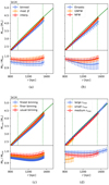 |
Fig. 1. Ideal clusters. Upper panels: cumulative total mass (calculated as the sum of gas mass and dark matter mass) with different models, binnings, and maximum radii for the cluster fulfilling perfect hydrostatic equilibrium. The green continuous line shows the true profile according to the simulations. The green vertical dotted lines show r500 and r200, which are computed based on the true profiles and the characteristic overdensity of the Universe at the corresponding redshift. The value of r200 is markedly larger than stated in Sect. 2.3, as the gas mass accounts for a considerable part of the total mass for the cluster fulfilling perfect hydrostatic equilibrium. Lower panels: ratio of fitted cumulative total mass and corresponding true mass. (a) different gas density models, (b) different dark matter mass models, (c) different binnings, (d) different maximum radii of the fit. |
4.2. Clusters from Magneticum Pathfinder simulations in idealized observations
In this section, we analyze the clusters from the Magneticum Pathfinder simulations under the idealized observational conditions. We use the input galactic absorption density of NH = 0.01 × 1022 cm−2. Deviating from Sect. 3.3, we only use seven energy bands for five clusters in snap 124 because the band with the highest energy does not include any counts.
We are particular interested in comparing the fitted and true mass profiles. Therefore, we define the parameter
 (8)
(8)
which we explore at certain radii. The values at the true r500 and r200 are called ζ500 and ζ200, respectively. We also write ζx for the ratio ζ at the corresponding rx. The fitted cumulative total masses at the exact values of the true r500 and r200 are calculated via linear interpolation between the values at the centers of the neighboring bins. The corresponding uncertainties are determined via linear interpolation between the lower (upper) limits of the uncertainties of the mass values at the neighboring bins. As mentioned in Sect. 3.3, for three of four clusters in snap 140, the fitted region cannot extend to the true r200. These clusters have the numbers 323, 89, and 83. The maximum radius of the fit lies somewhere between the true r500 and r200 in these cases. We therefore use a linear extrapolation of the fitted cumulative total mass profiles in logarithmic space to compute ζ200.
4.2.1. Different models and other factors
Similar to the approach for the idealized clusters (see Sect. 4.1), we analyze the effects of different models and other factors also for the clusters in snap 140 from the Magneticum Pathfinder simulations. These are the clusters with the lowest redshift. Figure 2 shows the values of ζ at the true r500 and r200. Those values at r200 that are based on an extrapolation of the profiles are shown as empty symbols. At r500, no extrapolation is necessary, as the fitted profiles reach this radius. Table 2 lists the individual values. From Fig. 2, one can see that the differences between the results using the interpolation model and the modified β-model are rather small at r500, whereas the results using the binned model diverge most from the others. The figure also shows that the results with the NFW and GNFW models do not significantly differ at r500 or r200. The small discrepancies might be due to the similar structure of the models. Furthermore, Fig. 2 shows the results with three different binnings. In the usual binning, one bin has a width of 10 pixels in the radial direction for snap 140 (the width of one pixel is 4 arcsec). In the finer binning, one bin has a width of 5 pixels, and in the finest binning, one bin has a width of 2 pixels. The total number of bins is then determined by the maximum radius of the fit; in the usual binning, it lies between 44 and 47 for the four clusters in snap 140. It can be seen that finer binnings do not guarantee better results. To investigate the influence of the position of the chosen center of the cluster, we repeat the fit taking the true minimum of the gravitational potential according to the simulations as the assumed center of the cluster (Fig. 2). The results assuming the true center position do not show systematically smaller differences from the results obtained when using the ideal value than those obtained when assuming the determined center according to Sect. 3.1. This indicates that choosing the region with the highest X-ray luminosity to be the center of the cluster works well in combination with the fitting process with MBProj2, probably as this choice of the center leads to a smoother decrease in the X-ray surface brightness with increasing radius.
 |
Fig. 2. Idealized observations: ζx at the corresponding true rx whilst varying models and other factors (different gas electron density models: interpolation model, modified β-model with one β-component, binned model (upper left); different dark-matter mass models: NFW model, GNFW model, Einasto model (upper right); different binnings (lower left); different center positions for the fit: determined center according to Sect. 3.1, true position of the minimum of the gravitational potential according to the simulations (lower right)). If not stated otherwise, we assume an interpolation model for the gas electron density and an NFW model for the dark-matter mass. The data points at the true r200 that are based on an extrapolation of the fitted profile are shown as empty symbols. More information can be found in the text. |
Comparison of results for idealized observations, varying models and other factors.
For the following analysis of the clusters from the Magneticum Pathfinder simulations in idealized observations, we use the interpolation model for the gas electron density. This model is most suitable for fitting the high data quality that the mentioned idealizations entail, as we deduce from the residual distribution of the fitted surface-brightness profiles (see Sect. 3.3). Furthermore, we use the NFW model for the dark-matter mass, because it mostly provides reliable results for a relatively low number of free parameters.
4.2.2. Fraction ζ
The results of the fits can be seen in the example of cluster 384 (snap 140) in Fig. 3. We compare the results of the fits with MBProj2 to the true profiles according to the simulations by investigating the fraction ζ (Eq. (8)) for all 93 clusters from the Magneticum Pathfinder simulations. The left panels of Fig. 4 show the distribution of ζx as a function of the true rx. The right panels show the corresponding results for the hydrostatic mass profiles according to theory (see Sect. 3.6). In all four panels, the individual values scatter around the ideal value of one, while the scattering amplitude varies between the different cases. Figure 5 shows the corresponding medians and 1σ intervals of the values in Fig. 4. The calculation of the 1σ intervals does not consider the uncertainties of the values for the individual clusters. All median values shown in Fig. 5 are between 0.77 and 0.99, which in principle fits our expectations of hydrostatic mass bias. The 1σ intervals for the results of the fits with MBProj2 are significantly larger than for the hydrostatic masses according to theory. This indicates not only that the validity of hydrostatic equilibrium is crucial for the mass determination, but also that the spectral analysis and the fitting process lead to additional uncertainties. One possible factor is the fact that our fit works with the two-dimensional projection of the cluster, whereas the true profiles, and therefore also the hydrostatic mass profiles according to theory, represent the three-dimensional quantities of the clusters. Another factor could be the shift of the center (see Sect. 3.5), which is further discussed in Sect. 4.2.5.
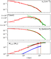 |
Fig. 3. Idealized observations: gas electron density, temperature, electron pressure, and cumulative mass as a function of the radius in physical kiloparsecs for cluster 384 in snap 140. In the first three panels, the red lines show the results of the fit with MBProj2. In the fourth panel, the red line shows the cumulative total mass and the blue line shows the cumulative gas mass according to the fit with MBProj2. The dashed orange line shows the linear extrapolation of the cumulative total mass profile. The green lines show the true profiles according to the simulations (for temperature and pressure: the dark green line represents the spectroscopic-like estimate of the profile (see Sect. 3.5); the light green line represents the mass-weighted profile). In the fourth panel, the green crosses show the true values of the cumulative total mass at the true r500 and r200. The black mass profile shows the hydrostatic mass according to theory (see Sect. 3.6); the green dotted line in the third panel shows the corresponding fit to the pressure profile. The vertical dotted lines in the fourth panel show the calculated values for r500, calculated and r200, calculated (red for the fit with MBProj2, orange for the extrapolation of the fit with MBProj2, and black for the hydrostatic profile according to theory). |
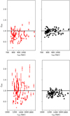 |
Fig. 4. Idealized observations: ζ at the true r500 (upper row) and r200 (lower row) for all 93 clusters from the Magneticum Pathfinder simulations. The two left panels show the results for the fits with MBProj2; the right panels show the results for the hydrostatic mass according to theory. |
4.2.3. Steepness of the mass profiles
It is apparent that the median value of ζ200 is higher than the median value of ζ500 for the results of the fit with MBProj2, whereas the opposite is true for the hydrostatic masses according to theory (Fig. 5). To further analyze this effect, we consider the “steepness” of the cumulative total mass profiles separately and define
 (9)
(9)
 |
Fig. 5. Idealized observations: medians and 1σ intervals of ζx for the profiles fitted with MBProj2 (left side) and for the hydrostatic mass according to theory (right side). |
In Eq. (9), we insert the true values of r500 and r200 and either the results of the fits for the cumulative total mass at these radii, or the corresponding results of the hydrostatic mass profiles according to theory, respectively (Fig. 6). For comparison, we show s, whilst inserting true values for masses and radii. Furthermore, we compute the corresponding median values and 1σ intervals (Fig. 7). The median s is too high for the fits with MBProj2, while the hydrostatic profiles according to theory are not sufficiently steep. The reason for the smaller values for the hydrostatic profiles according to theory could be the fact that they display features of the hydrostatic mass bias (compare to Lau et al. 2009). As the cluster fulfilling perfect hydrostatic equilibrium (see Sect. 4.1) has a profile that is not systematically too steep, we conclude that the excessively high s for many clusters according to the fit with MBProj2 is a consequence of the fit to the asymmetric and “clumpy” structure of the clusters from the Magneticum Pathfinder simulations (compare to results from observations; e.g., Simionescu et al. 2017). However, we do not find any unique characteristics of a cluster that certainly lead to excessive values of s. Furthermore, we are not able to solve the problem of excessive s by introducing priors to the model. Moreover, it seems to be unlikely that the high s for the fits with MBProj2 is caused by the hydrostatic mass bias, as the hydrostatic mass profiles according to theory show the opposite behavior.
 |
Fig. 6. Idealized observations: steepness parameter s for the 93 clusters from the Magneticum Pathfinder simulations as a function of the true r500. The left panel shows the results for the fits with MBProj2; the right panel shows the results for the hydrostatic mass according to theory. Both panels show the true values for comparison. We do not plot any uncertainties for s, as these are hard to determine because the uncertainties of the fitted values of M500 and M200 are correlated. |
 |
Fig. 7. Idealized observations: medians and 1σ intervals of s for the true cumulative mass profiles according to the simulations, for the profiles fitted with MBProj2, and for the hydrostatic mass profiles according to theory. |
4.2.4. Calculation of rx and Mx based on the mass profiles
In the next step, we compute values for r500, r200, and the cumulative total masses at these radii independently of the information from the simulations. In order to do this, we use the corresponding mass profiles and the critical density of the Universe at the corresponding redshift and calculate the radii, where the average overdensity of the cluster is 500 and 200 times the critical density, respectively (see Fig. 3). We use the same approach for the profiles fitted with MBProj2 and for the hydrostatic mass profiles according to theory, while for the former, we have to resort to a linear extrapolation in logarithmic space for some clusters. We denote the calculated values for the radii as rx,calculated. We also determine the corresponding masses at these radii Mx,calculated (Fig. 8). One can see that for most of the clusters, the calculated masses based on the fit with MBProj2 are smaller than the true masses; furthermore, they show a larger scattering amplitude. The uncertainty bars of Mx,calculated are determined according to the lower and upper limits of the fitted cumulative total mass profiles: considering the lower limit of the mass profile determines the lower uncertainty of each data point and vice versa. If Mx,calculated is calculated involving the extrapolation of the mass profile, the uncertainty of the mass profile in the outermost fitted bin is decisive.
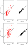 |
Fig. 8. Idealized observations: calculated mass values M500, calculated (upper row)/M200, calculated (lower row) as a function of true mass values according to the simulations M500/M200, respectively. The two left panels show the results for the fits with MBProj2; the right panels show the results for the hydrostatic mass according to theory. |
To compare the results of our calculation to the true values according to the simulations, we define two parameters:
 (10)
(10)
which we evaluate for x = 500 and x = 200. We note that rx and Mx denote the true values according to the simulations. The median values and 1σ intervals of γx and δx for our sample of clusters are shown in Fig. 9. Similarly to Fig. 5, the calculation of the 1σ intervals in Fig. 9 does not consider the uncertainties on the values for the individual clusters. The medians and 1σ intervals behave similarly to the corresponding values of ζx (see Fig. 5). Therefore, the fact that the median values of the results of the fits with MBProj2 are smaller than one is most likely a consequence of the hydrostatic mass bias. Moreover, the 1σ intervals for δx are much larger than for γx.
 |
Fig. 9. Idealized observations: medians and 1σ intervals of γx and δx (Eq. (10)). The red bars show the results for the fits with MBProj2; the black bars show the results for the hydrostatic profiles according to theory. |
4.2.5. Influence of the shift of the center
We mention in Sect. 3.5 that the shift of the center position might introduce discrepancies when comparing the profiles fitted with MBProj2 and the true profiles. To analyze this effect, we again show the fraction ζx, but this time as a function of the shift of the center divided by the true r500 (Fig. 10). Apart from the methodological influence, the size of the shift could also provide information about the properties of the cluster. Specifically, it is reasonable to assume that a larger shift often refers to a higher disturbance of the individual cluster (compare to e.g., Mohr et al. 1993; Poole et al. 2006; Rasia et al. 2013; Weißmann et al. 2013; Chon & Böhringer 2017). As the hydrostatic profiles according to theory are based on the true profiles, they also assume the true center position. This provides information about the correlation between the disturbance of the cluster and the validity of hydrostatic equilibrium. If the shift of the center is large compared to the true r500, one could expect the corresponding values of ζ to be far from one because the cluster might then be comparatively disturbed. In addition, this could produce systematic differences between the fitted and true profiles. Interestingly, a strong correlation between the normalized shift of the center and ζ is not discernible. This applies to both the results of the fit with MBProj2 and the hydrostatic profiles according to theory. Consequently, we cannot verify that the shift of the center as a measure of disturbance of a cluster is a substantial indicator for the validity of hydrostatic equilibrium. However, the position of the true center is a three-dimensional quantity, whereas the image-derived position is two-dimensional. This could lead to projection effects that smooth the correlation.
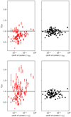 |
Fig. 10. Idealized observations: ζ at the true r500 (upper row) and r200 (lower row) as a function of the normalized shift of the center (see Sect. 3.5). The two left panels show the results for the fits with MBProj2; the right panels show the results for the hydrostatic mass according to theory. |
4.2.6. Evolution with redshift
To investigate the influence of the redshift on the results, we analyze the fraction ζ for the clusters in the different snaps separately (Fig. 11). The redshift of all clusters in the same snap is identical (see Sect. 2.2). The results of the fits are susceptible to statistical fluctuations due to low numbers of sources, leading to overly small median values for snap 136. Nevertheless, for the fits with MBProj2, an increase in the median value from ζ500 to ζ200 is discernible for every redshift. Therefore, the excessive steepness of the cumulative MBProj2 total mass profiles is apparent for all tested redshifts (see Sect. 4.2.3). In contrast, the results of the hydrostatic profiles according to theory reveal the opposite trend, which suggests that the influence of the hydrostatic mass bias is present for clusters with all tested redshifts. We do not find a clear trend of the medians with redshift.
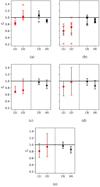 |
Fig. 11. Idealized observations: medians and 1σ intervals of ζx for each snap (comparable to Fig. 5). The results are shown at (1) r500 for the fits with MBProj2, (2) r200 for the fits with MBProj2, (3) r500 for the hydrostatic profiles according to theory and, (4) r200 for the hydrostatic profiles according to theory. The caption under each plot provides the number of the snap and the number of clusters it contains. Each cluster in a snap has the same redshift (see Table 1). Because of the low number of clusters in snaps 140 and 136, the corresponding plots also show the values for the individual clusters as crosses. (a) snap 140 (4 clusters), (b) snap 136 (6 clusters), (c) snap 132 (17 clusters), (d) snap 128 (27 clusters), (e) snap 124 (39 clusters). |
4.3. Clusters from Magneticum Pathfinder simulations in realistic observations
In this section, we analyze the clusters of our sample from the Magneticum Pathfinder simulations under realistic observational conditions. The X-ray data are generated in the eROSITA Final Equatorial Depth Survey (eFEDS) area (Brunner et al. 2022). eFEDS was observed in the performance verification phase of eROSITA. The clusters are produced to have the same true center position as for the idealized observations in Sect. 4.2. We assume the same center position as for the idealized observations and apply the same masking (both determined using idealized images; see Sects. 3.1 and 3.2). This would of course not be possible with real data, but ensures the results in Sect. 4.2 can be compared. For the realistic observations, we use the standard eROSITA PSF (Predehl et al. 2021; Merloni et al. 2012; Dauser et al. 2019). Furthermore, we use exposure maps with realistic exposure times. The exposure maps also take into account the eFEDS attitude data to model the pointing of the telescope over time. The version of the eROSITA instrument definition used is 1.8.2. Our background model makes use of the eFEDS survey data to make a particle background model and we incorporate an X-ray foreground model from Sanders et al. (2022). When fitting the synthetic data, we assume the survey average PSF. We do not include point sources in the synthetic data. We do not use the energy band with the highest energy for the realistic observations (see definition of energy band in Sect. 3.3). Figure 12 shows the same cluster under idealized and realistic observational conditions for comparison in the energy band 0.6 keV to 1.1 keV. The cluster is taken from snap 140, which is the snap with the lowest redshift.
 |
Fig. 12. Cluster 384 in snap 140 from the Magneticum Pathfinder simulations. The images use a logarithmic scale, cover energies from 0.6 keV to 1.1 keV, and are smoothed with a Gaussian. The numbers on the scales of the colorbars show the numbers of counts per pixel; they differ for idealized and realistic observations because of the relative exposure times. The green circles have a radius of about 3.1 arcmin and indicate the masked region. |
We assume a modified β-model with one β-component to model the electron gas density with MBProj2. This model appears to be more appropriate for realistic data quality than the interpolation model used in Sect. 4.2. For the dark-matter mass, we again use an NFW model. Background-surface-brightness profiles were created from cluster-free simulations using the same background model. When fitting the data, an extra parameter –which introduces a scaling between the model and fitted backgrounds levels– was included in the fits, with a Gaussian prior. Equivalent to Sect. 4.2, we assume that NH = 0.01 × 1022cm−2.
We analyze the data in the same way as in Sect. 4.2. Figure 13 shows the fraction ζ (Eq. (8)) for the clusters from the Magneticum Pathfinder simulations under realistic observational conditions. Figure 14 shows the corresponding medians and 1σ intervals. One can see that the uncertainty bars for the particular clusters are considerably larger than is the case for the idealized observations. This is in agreement with our expectations regarding the effects of the lower data quality. Further, the 1σ intervals of the total sample are larger. Moreover, the medians lie higher than for the idealized observations, particularly for ζ200.
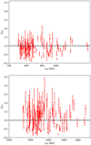 |
Fig. 13. Realistic observations: ζ at the true r500 (upper panel) and r200 (lower panel), according to the fits with MBProj2. |
 |
Fig. 14. Realistic observations: medians and 1σ intervals of ζx, according to the fits with MBProj2. |
Next, we analyze the steepness value s (Eq. (9)) of the cumulative total mass profiles. Figure 15 shows the results for the particular clusters on the left and the corresponding median and 1σ interval on the right. The median of s is clearly higher than for the idealized observations. Apparently the lower data quality magnifies the problem of the excessive steepness, probably also as we are forced to use the modified β-model with one β component instead of the interpolation model for the density. In contrast to the median, the highest values of s are very similar for idealized and realistic observational conditions.
 |
Fig. 15. Realistic observations: steepness parameter s for the results of the fits with MBProj2 and the true values for comparison. The horizontal red line shows the median for the results of the fits; the red region shows the corresponding 1σ interval. This plot can be compared to Fig. 6. |
As for the idealized observations, we compute values for rx,calculated and Mx,calculated based on the cumulative total mass profiles also for the realistic observations (see Sect. 4.2.4). The calculated mass values for the individual clusters are shown in Fig. 16. Figure 17 shows the medians and 1σ intervals of γ and δ (Eq. (10)) for the realistic observations. The medians of γ200 and δ200 are remarkably higher than for the idealized observations; the 1σ intervals are considerably larger in all cases. The extremely large 1σ interval of δ200 is probably also due to the fact that all values where the corresponding r200, calculated is substantially larger than the true r200 are based on a linear extrapolation of the fitted cumulative-total-mass profile (compare to Sect. 4.2.4). The excessive steepness of the mass profile then leads to excessive steepness of the extrapolation over a large radius range. This causes overly large values of r200, calculated and has even stronger implications for M200, calculated.
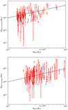 |
Fig. 16. Realistic observations: calculated mass values M500, calculated (upper panel) and M200, calculated (lower panel), based on the fits with MBProj2, as a function of true mass values according to the simulations M500 and M200, respectively. |
 |
Fig. 17. Realistic observations: medians and 1σ intervals of γx and δx (Eq. (10)), based on the fits with MBProj2. |
Insight may be gained by analyzing the fraction ζ independently for each redshift again for the realistic observations (Fig. 18). We find that the trend toward systematically excessive medians of ζ200 is only discernible for the clusters in the snaps 128 and 124. For lower redshifts, the results are close to our expectations, neglecting some outliers in snap 136. Also, the medians for ζ500 for higher redshifts seem to be plausible. In contrast, the reaction of the fit to the realistic data quality causes excessive steepness particularly for higher redshifts, and therefore leads to unreasonably high values of ζ200. Although the problem of excessive steepness also exists for the idealized observations, the medians of ζ200 show reasonable values there, even for high redshifts.
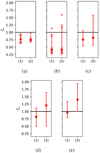 |
Fig. 18. Realistic observations: medians and 1σ intervals of ζx for each snap (comparable to Fig. 14). The results are shown at (1) r500 for the fits with MBProj2 and (2) r200 for the fits with MBProj2. Each cluster in a snap has the same redshift (see Table 1). Because of the low number of clusters in snaps 140 and 136, the corresponding plots also show the values for the individual clusters as crosses. (a) snap 140, (b) snap 136, (c) snap 132, (d) snap 128, (e) snap 124. |
5. Discussion
Our results for the fits with MBProj2 are partially based on knowledge from the simulations, such as the true values for r500 and r200. Specifically, we use a radius close to the true r200 as the maximum radius for the fit (see Sect. 3.3). To avoid the influences of this choice, we perform the analysis of ζ at the true r500 and r200 for the clusters from the Magneticum Pathfinder simulations using a value for the maximum radius that is estimated by eye to roughly match r200. This estimate is based on the image of the cluster and naturally deviates from the true value for some clusters. All these estimated radii are larger than the true r500, but some of them are smaller than the true r200. In this case, we determine ζ at the true r200 using a linear extrapolation in logarithmic space. As in the previous section, we determine the corresponding values for ζ at the true r500 and r200. For idealized observational conditions, we find that the corresponding median of ζ500 deviates from the value in the previous section (see Fig. 5) by less than 0.5%; for the median of ζ200 we find a deviation of about 5%. For realistic observational conditions, the corresponding deviations are about 1% at r500 and about 4% at r200. Also, the 1σ intervals are mostly similar for both choices of maximum radius for the fit.
Barnes et al. (2021) also derive hydrostatic masses of galaxy clusters based on simulations, including clusters in a similar mass range. Further, these authors also investigate the fraction of hydrostatic mass over true mass. They find median values and 1σ intervals in the same order of magnitude as our results, assuming idealized observational conditions. The authors also find the hydrostatic mass bias to be mass dependent. In our results, a clear dependence of the fraction ζ on the radius of the cluster is not discernible. Nevertheless, our results for the hydrostatic mass bias obtained with the fit with MBProj2 seem to be affected by the problem of excessive steepness.
We recognize that it is difficult to predict whether or not results for a cluster will be close to the true values by looking at the image of the cluster. As a dependence of ζ on the relative shift of the center is not clearly visible, we suspect that additional as aspects have an influence on the results, such as the degree of symmetry of the cluster (see e.g., Piffaretti et al. 2003; Morandi et al. 2010; Eckert et al. 2015). The validity of hydrostatic equilibrium in the clusters could also be affected by mergers (see e.g., Nelson et al. 2012; Reiprich et al. 2004; Puchwein & Bartelmann 2007). To gain more knowledge about individual clusters and the validity of the assumption of hydrostatic equilibrium, hydrostatic masses can be compared to the results of other measurements (Ettori et al. 2019), such as X-ray-based scaling relations (Vikhlinin et al. 2009), galaxy dynamics (Zhang et al. 2017; Rines et al. 2016), weak lensing (Zhang et al. 2010), and the Sunyaev–Zeldovich effect (Kay et al. 2012). Ettori et al. (2019) identified the masses of several different measurements to be mostly congruent with the results based on the assumption of hydrostatic equilibrium.
6. Conclusions
We investigated hydrostatic equilibrium in clusters of galaxies using a sample of 93 clusters from the Magneticum Pathfinder simulations as well as several clusters with idealized properties. We fit hydrostatic models to the X-ray images of the clusters using the fitting code MBProj2, while testing different models for the electron density in the ICM and for the dark-matter mass. For comparison, we computed hydrostatic mass profiles using the true profiles for gas electron density and pressure known from the simulations. We draw the following conclusions from our findings:
-
Assuming isothermal clusters with different temperatures under idealized observational conditions, MBProj2 is able to fit flat temperature profiles that deviate from the true values by a few percent at the most; for the majority of cases, the deviations are at about 1% or smaller.
-
Under idealized observational conditions, the cumulative total mass profile of a cluster fulfilling perfect hydrostatic equilibrium can be reproduced such that the deviations of the cumulative total mass at the true r500 and r200 are below 7%; this holds for all tested models.
-
Considering the clusters from the Magneticum Pathfinder simulations under idealized observational conditions and assuming a modified β-model with one β component for the gas electron density and an NFW model for the dark matter mass, the fit with MBProj2 leads to medians for the fraction ζ (Eq. (8)) that are between 0.77 and 0.9, which roughly agrees with our expectations of b ∼ 0.1 − 0.2 as found from simulations (see Sect. 1). The 1σ interval for ζ500 has an adequate size, while the results for ζ200 exhibit a noticeably larger scattering amplitude. Furthermore, we observe excessive steepness of the fitted cumulative mass profiles on average.
-
The hydrostatic mass profiles based on theory show results that match our assumptions for almost all clusters: The medians of ζ500 and ζ200 are congruent with the expectations and the corresponding 1σ intervals are considerably smaller than for the fit with MBProj2.
-
The shift of the center position, which might be used as a proxy for the dynamic state of a cluster, does not make a substantial difference in the accuracy of hydrostatic masses in our case.
-
Considering realistic eROSITA data quality, we find medians and 1σ intervals for ζ500 that are consistent with our expectations; for ζ200 we find excessive medians for clusters with higher redshifts.
-
The values for r500, calculated, r200, calculated, M500, calculated and M200, calculated –calculated based on the cumulative mass profiles and the critical density of the Universe at the corresponding redshift– show reasonable medians for idealized observational conditions; however, they also seem to be affected by the problem of excessive steepness of the fitted cumulative total mass profiles. For realistic observational conditions, the magnified steepness problem leads to overly high medians of γ200 and δ200 (see Eq. (10)); these two quantities further show unreasonably large 1σ intervals, probably also driven by the extrapolation of the profiles.
-
Hydrostatic masses obtained with MBProj2 are an interesting and helpful resource by themselves, but also in the context of the eROSITA survey.
A future application of mass measurements of galaxy clusters with MBProj2 could be in cosmological studies, as already mentioned in Sect. 1. For this, the code will be applied to real data from eROSITA. The exact behavior of the fit as well as further issues with real data could be the subject of future work. Furthermore, we may wish to compare the results from real data to the results obtained with Chandra and XMM-Newton and to those from weak lensing. In summary, there are a number of interesting prospective projects that are likely to yield insightful information.
Acknowledgments
The Magneticum Pathfinder simulations have been performed at the Leibniz-Rechenzentrum with CPU time assigned to the projects pr86re and pr83li. The synthetic data shown here were processed using the eSASS software system developed by the German eROSITA consortium. KD acknowledges support by the COMPLEX project from the European Research Council (ERC) under the European Union’s Horizon 2020 research and innovation program grant agreement ERC-2019-AdG 882679 and support by the Deutsche Forschungsgemeinschaft (DFG, German Research Foundation) under Germany’s Excellence Strategy – EXC-2094 – 390783311. VB acknowledges support by the DFG project nr. 415510302. EB acknowledges financial support from the European Research Council (ERC) Consolidator Grant under the European Union’s Horizon 2020 research and innovation programme (grant agreement CoG DarkQuest No 101002585). Parts of the content are identical or similar to the master’s thesis “Mass Profiles of Galaxy Clusters in the eROSITA survey” by Dominik Scheck, submitted on October 19, 2021 at the Department of Physics of the Technical University of Munich.
References
- Anders, E., & Grevesse, N. 1989, Geochim. Cosmochim. Acta, 53, 197 [Google Scholar]
- Arnaud, K. A. 1996, in Astronomical Data Analysis Software and Systems V, eds. G. H. Jacoby, & J. Barnes, ASP Conf. Ser., 101, 17 [NASA ADS] [Google Scholar]
- Balucinska-Church, M., & McCammon, D. 1992, ApJ, 400, 699 [Google Scholar]
- Barnes, D. J., Vogelsberger, M., Pearce, F. A., et al. 2021, MNRAS, 506, 2533 [NASA ADS] [CrossRef] [Google Scholar]
- Biffi, V., Dolag, K., Böhringer, H., & Lemson, G. 2012, MNRAS, 420, 3545 [NASA ADS] [Google Scholar]
- Biffi, V., Dolag, K., & Böhringer, H. 2013, MNRAS, 428, 1395 [Google Scholar]
- Biffi, V., Borgani, S., Murante, G., et al. 2016, ApJ, 827, 112 [NASA ADS] [CrossRef] [Google Scholar]
- Biffi, V., Dolag, K., & Merloni, A. 2018, MNRAS, 481, 2213 [Google Scholar]
- Biffi, V., Dolag, K., Reiprich, T. H., et al. 2022, A&A, 661, A17 [Google Scholar]
- Boehringer, H., & Werner, N. 2009, ArXiv e-prints [arXiv:0907.4277] [Google Scholar]
- Brunner, H., Boller, T., Coutinho, D., et al. 2018, in Space Telescopes and Instrumentation 2018: Ultraviolet to Gamma Ray, eds. J. W. A. den Herder, S. Nikzad, & K. Nakazawa, SPIE Conf. Ser., 10699, 106995G [NASA ADS] [Google Scholar]
- Brunner, H., Liu, T., Lamer, G., et al. 2022, A&A, 661, A1 [NASA ADS] [CrossRef] [EDP Sciences] [Google Scholar]
- Bryan, G. L., & Norman, M. L. 1998, ApJ, 495, 80 [NASA ADS] [CrossRef] [Google Scholar]
- Bulbul, E., Liu, A., Pasini, T., et al. 2022, A&A, 661, A10 [NASA ADS] [CrossRef] [EDP Sciences] [Google Scholar]
- Cavaliere, A., & Fusco-Femiano, R. 1978, A&A, 70, 677 [NASA ADS] [Google Scholar]
- Chiu, I., Mohr, J., McDonald, M., et al. 2016, MNRAS, 455, 258 [NASA ADS] [CrossRef] [Google Scholar]
- Chiu, I. N., Ghirardini, V., Liu, A., et al. 2022, A&A, 661, A11 [NASA ADS] [CrossRef] [EDP Sciences] [Google Scholar]
- Chon, G., & Böhringer, H. 2017, A&A, 606, L4 [NASA ADS] [CrossRef] [EDP Sciences] [Google Scholar]
- Clerc, N., Ramos-Ceja, M. E., Ridl, J., et al. 2018, A&A, 617, A92 [NASA ADS] [CrossRef] [EDP Sciences] [Google Scholar]
- Dauser, T., Falkner, S., Lorenz, M., et al. 2019, A&A, 630, A66 [NASA ADS] [CrossRef] [EDP Sciences] [Google Scholar]
- Eckert, D., Roncarelli, M., Ettori, S., et al. 2015, MNRAS, 447, 2198 [Google Scholar]
- Ettori, S., Donnarumma, A., Pointecouteau, E., et al. 2013, Space Sci. Rev., 177, 119 [Google Scholar]
- Ettori, S., Ghirardini, V., Eckert, D., et al. 2019, A&A, 621, A39 [NASA ADS] [CrossRef] [EDP Sciences] [Google Scholar]
- Foreman-Mackey, D., Hogg, D. W., Lang, D., & Goodman, J. 2013, PASP, 125, 306 [Google Scholar]
- George, I. M., Arnaud, K. A., Pence, B., Ruamsuwan, L., & Corcoran, M. F. 2007, The Calibration Requirements for Spectral Analysis (Definition of RMF and ARF file formats), Technical report, Code 662, NASA/GSFC, Greenbelt, MD20771 [Google Scholar]
- Ghirardini, V., Ettori, S., Eckert, D., et al. 2018, A&A, 614, A7 [NASA ADS] [CrossRef] [EDP Sciences] [Google Scholar]
- Goodman, J., & Weare, J. 2010, Commun. Appl. Math. Comput. Sci., 5, 65 [Google Scholar]
- Grandis, S., Bocquet, S., Mohr, J. J., Klein, M., & Dolag, K. 2021, MNRAS, 507, 5671 [NASA ADS] [CrossRef] [Google Scholar]
- Hoekstra, H., Herbonnet, R., Muzzin, A., et al. 2015, MNRAS, 449, 685 [NASA ADS] [CrossRef] [Google Scholar]
- Kay, S. T., Peel, M. W., Short, C. J., et al. 2012, MNRAS, 422, 1999 [NASA ADS] [CrossRef] [Google Scholar]
- Komatsu, E., Smith, K. M., Dunkley, J., et al. 2011, ApJS, 192, 18 [Google Scholar]
- Lau, E. T., Kravtsov, A. V., & Nagai, D. 2009, ApJ, 705, 1129 [NASA ADS] [CrossRef] [Google Scholar]
- Lau, E. T., Nagai, D., & Nelson, K. 2013, ApJ, 777, 151 [NASA ADS] [CrossRef] [Google Scholar]
- Liu, A., Bulbul, E., Ghirardini, V., et al. 2022, A&A, 661, A2 [NASA ADS] [CrossRef] [EDP Sciences] [Google Scholar]
- Martino, R., Mazzotta, P., Bourdin, H., et al. 2014, MNRAS, 443, 2342 [NASA ADS] [CrossRef] [Google Scholar]
- Mazzotta, P., Rasia, E., Moscardini, L., & Tormen, G. 2004, MNRAS, 354, 10 [NASA ADS] [CrossRef] [Google Scholar]
- Merloni, A., Predehl, P., Becker, W., et al. 2012, ArXiv e-prints [arXiv:1209.3114] [Google Scholar]
- Mohr, J. J., Fabricant, D. G., & Geller, M. J. 1993, ApJ, 413, 492 [Google Scholar]
- Morandi, A., Pedersen, K., & Limousin, M. 2010, ApJ, 713, 491 [NASA ADS] [CrossRef] [Google Scholar]
- Morrison, R., & McCammon, D. 1983, ApJ, 270, 119 [Google Scholar]
- Navarro, J. F., Frenk, C. S., & White, S. D. M. 1996, ApJ, 462, 563 [Google Scholar]
- Nelson, K., Rudd, D. H., Shaw, L., & Nagai, D. 2012, ApJ, 751, 121 [NASA ADS] [CrossRef] [Google Scholar]
- Piffaretti, R., Jetzer, P., & Schindler, S. 2003, A&A, 398, 41 [NASA ADS] [CrossRef] [EDP Sciences] [Google Scholar]
- Pillepich, A., Porciani, C., & Reiprich, T. H. 2012, MNRAS, 422, 44 [Google Scholar]
- Pointecouteau, E., Arnaud, M., Kaastra, J., & de Plaa, J. 2004, A&A, 423, 33 [NASA ADS] [CrossRef] [EDP Sciences] [Google Scholar]
- Pointecouteau, E., Arnaud, M., & Pratt, G. W. 2005, A&A, 435, 1 [NASA ADS] [CrossRef] [EDP Sciences] [Google Scholar]
- Poole, G. B., Fardal, M. A., Babul, A., et al. 2006, MNRAS, 373, 881 [Google Scholar]
- Pratt, G. W., Arnaud, M., Biviano, A., et al. 2019, Space Sci. Rev., 215, 25 [Google Scholar]
- Predehl, P., Andritschke, R., Arefiev, V., et al. 2021, A&A, 647, A1 [EDP Sciences] [Google Scholar]
- Puchwein, E., & Bartelmann, M. 2007, A&A, 474, 745 [NASA ADS] [CrossRef] [EDP Sciences] [Google Scholar]
- Rasia, E., Meneghetti, M., & Ettori, S. 2013, The Astron. Rev., 8, 40 [NASA ADS] [Google Scholar]
- Reiprich, T. H., Sarazin, C. L., Kempner, J. C., & Tittley, E. 2004, ApJ, 608, 179 [Google Scholar]
- Retana-Montenegro, E., van Hese, E., Gentile, G., Baes, M., & Frutos-Alfaro, F. 2012, A&A, 540, A70 [NASA ADS] [CrossRef] [EDP Sciences] [Google Scholar]
- Rines, K. J., Geller, M. J., Diaferio, A., & Hwang, H. S. 2016, ApJ, 819, 63 [NASA ADS] [CrossRef] [Google Scholar]
- Sanders, J. S., Fabian, A. C., Hlavacek-Larrondo, J., et al. 2014, MNRAS, 444, 1497 [NASA ADS] [CrossRef] [Google Scholar]
- Sanders, J. S., Fabian, A. C., Russell, H. R., & Walker, S. A. 2018, MNRAS, 474, 1065 [NASA ADS] [CrossRef] [Google Scholar]
- Sanders, J. S., Biffi, V., Brüggen, M., et al. 2022, A&A, 661, A36 [NASA ADS] [CrossRef] [EDP Sciences] [Google Scholar]
- Schellenberger, G., Reiprich, T. H., Lovisari, L., Nevalainen, J., & David, L. 2015, A&A, 575, A30 [NASA ADS] [CrossRef] [EDP Sciences] [Google Scholar]
- Schmidt, R. W., & Allen, S. W. 2007, MNRAS, 379, 209 [NASA ADS] [CrossRef] [Google Scholar]
- Schoenberg, I. J. 1964, Proc. Nat. Acad. Sci., 51, 24 [NASA ADS] [CrossRef] [Google Scholar]
- Simionescu, A., Werner, N., Mantz, A., Allen, S. W., & Urban, O. 2017, MNRAS, 469, 1476 [Google Scholar]
- Smith, R. K., Brickhouse, N. S., Liedahl, D. A., & Raymond, J. C. 2001, ApJ, 556, L91 [Google Scholar]
- Springel, V., & Hernquist, L. 2003a, in Astrophysical Supercomputing using Particle Simulations, eds. J. Makino, & P. Hut, 208, 273 [NASA ADS] [Google Scholar]
- Springel, V., & Hernquist, L. 2003b, MNRAS, 339, 289 [Google Scholar]
- Springel, V., & Hernquist, L. 2003c, MNRAS, 339, 312 [NASA ADS] [CrossRef] [Google Scholar]
- Tanabashi, M., Hagiwara, K., Hikasa, K., et al. 2018, Phys. Rev. D, 98, 030001 [CrossRef] [Google Scholar]
- Tornatore, L., Borgani, S., Matteucci, F., Recchi, S., & Tozzi, P. 2004, MNRAS, 349, L19 [Google Scholar]
- Tornatore, L., Borgani, S., Dolag, K., & Matteucci, F. 2007, MNRAS, 382, 1050 [Google Scholar]
- Vikhlinin, A. 2006, ApJ, 640, 710 [NASA ADS] [CrossRef] [Google Scholar]
- Vikhlinin, A., Forman, W., & Jones, C. 1999, ApJ, 525, 47 [NASA ADS] [CrossRef] [Google Scholar]
- Vikhlinin, A., Kravtsov, A., Forman, W., et al. 2006, ApJ, 640, 691 [Google Scholar]
- Vikhlinin, A., Burenin, R. A., Ebeling, H., et al. 2009, ApJ, 692, 1033 [Google Scholar]
- von der Linden, A., Allen, M. T., Applegate, D. E., et al. 2014, MNRAS, 439, 2 [NASA ADS] [CrossRef] [Google Scholar]
- Weißmann, A., Böhringer, H., Šuhada, R., & Ameglio, S. 2013, A&A, 549, A19 [NASA ADS] [CrossRef] [EDP Sciences] [Google Scholar]
- Wyithe, J. S. B., Turner, E. L., & Spergel, D. N. 2001, ApJ, 555, 504 [NASA ADS] [CrossRef] [Google Scholar]
- Zhang, Y.-Y., Okabe, N., Finoguenov, A., et al. 2010, ApJ, 711, 1033 [NASA ADS] [CrossRef] [Google Scholar]
- Zhang, Y.-Y., Reiprich, T. H., Schneider, P., et al. 2017, A&A, 599, A138 [NASA ADS] [CrossRef] [EDP Sciences] [Google Scholar]
- Zhao, H. 1996, MNRAS, 278, 488 [Google Scholar]
All Tables
Distribution of clusters among five snapshots in the Magneticum Pathfinder simulations.
Comparison of results for idealized observations, varying models and other factors.
All Figures
 |
Fig. 1. Ideal clusters. Upper panels: cumulative total mass (calculated as the sum of gas mass and dark matter mass) with different models, binnings, and maximum radii for the cluster fulfilling perfect hydrostatic equilibrium. The green continuous line shows the true profile according to the simulations. The green vertical dotted lines show r500 and r200, which are computed based on the true profiles and the characteristic overdensity of the Universe at the corresponding redshift. The value of r200 is markedly larger than stated in Sect. 2.3, as the gas mass accounts for a considerable part of the total mass for the cluster fulfilling perfect hydrostatic equilibrium. Lower panels: ratio of fitted cumulative total mass and corresponding true mass. (a) different gas density models, (b) different dark matter mass models, (c) different binnings, (d) different maximum radii of the fit. |
| In the text | |
 |
Fig. 2. Idealized observations: ζx at the corresponding true rx whilst varying models and other factors (different gas electron density models: interpolation model, modified β-model with one β-component, binned model (upper left); different dark-matter mass models: NFW model, GNFW model, Einasto model (upper right); different binnings (lower left); different center positions for the fit: determined center according to Sect. 3.1, true position of the minimum of the gravitational potential according to the simulations (lower right)). If not stated otherwise, we assume an interpolation model for the gas electron density and an NFW model for the dark-matter mass. The data points at the true r200 that are based on an extrapolation of the fitted profile are shown as empty symbols. More information can be found in the text. |
| In the text | |
 |
Fig. 3. Idealized observations: gas electron density, temperature, electron pressure, and cumulative mass as a function of the radius in physical kiloparsecs for cluster 384 in snap 140. In the first three panels, the red lines show the results of the fit with MBProj2. In the fourth panel, the red line shows the cumulative total mass and the blue line shows the cumulative gas mass according to the fit with MBProj2. The dashed orange line shows the linear extrapolation of the cumulative total mass profile. The green lines show the true profiles according to the simulations (for temperature and pressure: the dark green line represents the spectroscopic-like estimate of the profile (see Sect. 3.5); the light green line represents the mass-weighted profile). In the fourth panel, the green crosses show the true values of the cumulative total mass at the true r500 and r200. The black mass profile shows the hydrostatic mass according to theory (see Sect. 3.6); the green dotted line in the third panel shows the corresponding fit to the pressure profile. The vertical dotted lines in the fourth panel show the calculated values for r500, calculated and r200, calculated (red for the fit with MBProj2, orange for the extrapolation of the fit with MBProj2, and black for the hydrostatic profile according to theory). |
| In the text | |
 |
Fig. 4. Idealized observations: ζ at the true r500 (upper row) and r200 (lower row) for all 93 clusters from the Magneticum Pathfinder simulations. The two left panels show the results for the fits with MBProj2; the right panels show the results for the hydrostatic mass according to theory. |
| In the text | |
 |
Fig. 5. Idealized observations: medians and 1σ intervals of ζx for the profiles fitted with MBProj2 (left side) and for the hydrostatic mass according to theory (right side). |
| In the text | |
 |
Fig. 6. Idealized observations: steepness parameter s for the 93 clusters from the Magneticum Pathfinder simulations as a function of the true r500. The left panel shows the results for the fits with MBProj2; the right panel shows the results for the hydrostatic mass according to theory. Both panels show the true values for comparison. We do not plot any uncertainties for s, as these are hard to determine because the uncertainties of the fitted values of M500 and M200 are correlated. |
| In the text | |
 |
Fig. 7. Idealized observations: medians and 1σ intervals of s for the true cumulative mass profiles according to the simulations, for the profiles fitted with MBProj2, and for the hydrostatic mass profiles according to theory. |
| In the text | |
 |
Fig. 8. Idealized observations: calculated mass values M500, calculated (upper row)/M200, calculated (lower row) as a function of true mass values according to the simulations M500/M200, respectively. The two left panels show the results for the fits with MBProj2; the right panels show the results for the hydrostatic mass according to theory. |
| In the text | |
 |
Fig. 9. Idealized observations: medians and 1σ intervals of γx and δx (Eq. (10)). The red bars show the results for the fits with MBProj2; the black bars show the results for the hydrostatic profiles according to theory. |
| In the text | |
 |
Fig. 10. Idealized observations: ζ at the true r500 (upper row) and r200 (lower row) as a function of the normalized shift of the center (see Sect. 3.5). The two left panels show the results for the fits with MBProj2; the right panels show the results for the hydrostatic mass according to theory. |
| In the text | |
 |
Fig. 11. Idealized observations: medians and 1σ intervals of ζx for each snap (comparable to Fig. 5). The results are shown at (1) r500 for the fits with MBProj2, (2) r200 for the fits with MBProj2, (3) r500 for the hydrostatic profiles according to theory and, (4) r200 for the hydrostatic profiles according to theory. The caption under each plot provides the number of the snap and the number of clusters it contains. Each cluster in a snap has the same redshift (see Table 1). Because of the low number of clusters in snaps 140 and 136, the corresponding plots also show the values for the individual clusters as crosses. (a) snap 140 (4 clusters), (b) snap 136 (6 clusters), (c) snap 132 (17 clusters), (d) snap 128 (27 clusters), (e) snap 124 (39 clusters). |
| In the text | |
 |
Fig. 12. Cluster 384 in snap 140 from the Magneticum Pathfinder simulations. The images use a logarithmic scale, cover energies from 0.6 keV to 1.1 keV, and are smoothed with a Gaussian. The numbers on the scales of the colorbars show the numbers of counts per pixel; they differ for idealized and realistic observations because of the relative exposure times. The green circles have a radius of about 3.1 arcmin and indicate the masked region. |
| In the text | |
 |
Fig. 13. Realistic observations: ζ at the true r500 (upper panel) and r200 (lower panel), according to the fits with MBProj2. |
| In the text | |
 |
Fig. 14. Realistic observations: medians and 1σ intervals of ζx, according to the fits with MBProj2. |
| In the text | |
 |
Fig. 15. Realistic observations: steepness parameter s for the results of the fits with MBProj2 and the true values for comparison. The horizontal red line shows the median for the results of the fits; the red region shows the corresponding 1σ interval. This plot can be compared to Fig. 6. |
| In the text | |
 |
Fig. 16. Realistic observations: calculated mass values M500, calculated (upper panel) and M200, calculated (lower panel), based on the fits with MBProj2, as a function of true mass values according to the simulations M500 and M200, respectively. |
| In the text | |
 |
Fig. 17. Realistic observations: medians and 1σ intervals of γx and δx (Eq. (10)), based on the fits with MBProj2. |
| In the text | |
 |
Fig. 18. Realistic observations: medians and 1σ intervals of ζx for each snap (comparable to Fig. 14). The results are shown at (1) r500 for the fits with MBProj2 and (2) r200 for the fits with MBProj2. Each cluster in a snap has the same redshift (see Table 1). Because of the low number of clusters in snaps 140 and 136, the corresponding plots also show the values for the individual clusters as crosses. (a) snap 140, (b) snap 136, (c) snap 132, (d) snap 128, (e) snap 124. |
| In the text | |
Current usage metrics show cumulative count of Article Views (full-text article views including HTML views, PDF and ePub downloads, according to the available data) and Abstracts Views on Vision4Press platform.
Data correspond to usage on the plateform after 2015. The current usage metrics is available 48-96 hours after online publication and is updated daily on week days.
Initial download of the metrics may take a while.


