| Issue |
A&A
Volume 667, November 2022
|
|
|---|---|---|
| Article Number | A87 | |
| Number of page(s) | 22 | |
| Section | Extragalactic astronomy | |
| DOI | https://doi.org/10.1051/0004-6361/202243612 | |
| Published online | 09 November 2022 | |
The edges of galaxies: Tracing the limits of star formation
1
The Oskar Klein Centre, Department of Astronomy, Stockholm University, AlbaNova, 10691 Stockholm, Sweden
e-mail: nushkia.chamba@astro.su.se
2
Instituto de Astrofísica de Canarias (IAC), 38205 La Laguna, Tenerife, Spain
3
Departmento de Astrofísica, Universidad de La Laguna (ULL), 38200 La Laguna, Tenerife, Spain
Received:
22
March
2022
Accepted:
7
September
2022
The outskirts of galaxies have been studied from multiple perspectives for the past few decades. However, it is still unknown if all galaxies have clear-cut edges similar to everyday objects. We address this question by developing physically motivated criteria to define the edges of galaxies. Based on the gas density threshold required for star formation, we define the edge of a galaxy as the outermost radial location associated with a significant drop in either past or ongoing in situ star formation. We explore ∼1000 low-inclination galaxies with a wide range in morphology (dwarfs to ellipticals) and stellar mass (107 M⊙ < M⋆ < 1012 M⊙). The location of the edges of these galaxies (Redge) were visually identified as the outermost cutoff or truncation in their radial profiles using deep multi-band optical imaging from the IAC Stripe82 Legacy Project. We find this characteristic feature at the following mean stellar mass density, which varies with galaxy morphology: 2.9 ± 0.10 M⊙ pc−2 for ellipticals, 1.1 ± 0.04 M⊙ pc−2 for spirals, and 0.6 ± 0.03 M⊙ pc−2 for present-day star-forming dwarfs. Additionally, we find that Redge depends on its age (colour) where bluer galaxies have larger Redge at a fixed stellar mass. The resulting stellar mass–size plane using Redge as a physically motivated galaxy size measure has a very narrow intrinsic scatter (≲0.06 dex). These results highlight the importance of new deep imaging surveys to explore the growth of galaxies and trace the limits of star formation in their outskirts.
Key words: galaxies: fundamental parameters / galaxies: photometry / galaxies: formation / methods: data analysis / methods: observational / techniques: photometric
© N. Chamba et al. 2022
 Open Access article, published by EDP Sciences, under the terms of the Creative Commons Attribution License (https://creativecommons.org/licenses/by/4.0), which permits unrestricted use, distribution, and reproduction in any medium, provided the original work is properly cited.
This article is published in open access under the Subscribe-to-Open model. Subscribe to A&A to support open access publication.
1. Introduction
Galaxies grow and evolve through two main channels: in situ star formation via the conversion of gas into stars and ex situ stellar and gas accretion via merging and interactive events with its neighbourhood (e.g., Toomre & Toomre 1972; White & Rees 1978; Efstathiou & Silk 1983). While merging events are expected to happen predominantly in the most massive galaxies, current stellar mass growth via in situ star formation occurs in the majority of dwarfs and spiral galaxies, and it depends on the density of gas in these systems. In other words, stars can form in a galaxy as long as the density of gas surpasses a critical threshold (e.g., Quirk 1972; Fall & Efstathiou 1980; Kennicutt 1989; Schaye 2004). The radial location of the ‘edge’ of star formation as defined by this critical gas density threshold in a galaxy is thus a physically meaningful way to study the growth and evolution of galaxies.
This idea has recently been proposed by Trujillo et al. (2020) and Chamba et al. (2020) as a new, physically motivated definition of galaxy size (see also Chamba 2020, for a historical review on galaxy size measures). To make this definition operative, in these studies, we specifically chose a stellar mass density of 1 M⊙ pc−2 as a proxy to locate the gas density threshold required for star formation in galaxies based on theoretical (e.g., Schaye 2004) and observational (e.g., Martínez-Lombilla et al. 2019) evidence. This statement is based on the abrupt drop in the ultra-violet radial profiles of two Milky-Way-like galaxies reported by Martínez-Lombilla et al. (2019) in the region where their stellar mass density profiles are truncated (at 1 M⊙ pc−2 after correcting for inclination). Consequently, the radial location of this isomass contour was used as a size measure (dubbed R1), which is uniquely associated with the visual location of the edges of galaxies. Trujillo et al. (2020) have recently shown that the resulting size–stellar mass relation over five orders of magnitude in stellar mass (107 M⊙ < M⋆ < 1012 M⊙) produced an extremely tight distribution, with an intrinsic scatter (i.e. 0.06 dex) three times smaller than when using the de Vaucouleurs (1948) effective radius, which is a popular measure for galaxy size defined as the radius that encloses half the total light of a galaxy. Furthermore, Chamba et al. (2020) show that, in contrast to the effective radius that depends on the concentration of light in galaxies, R1 is a much better representation of the boundaries of galaxies to fairly compare the sizes of distinctive galaxy populations or morphologies whose light distributions are very different.
While the above results are very promising, the truncation at 1 M⊙ pc−2 has thus far only been observed at the edges of Milky-Way-like disk galaxies (Martínez-Lombilla et al. 2019). As the exact stellar mass surface density depends on the efficiency of transforming gas into stars, the fixed value at 1 M⊙ pc−2 cannot be assumed to hold for galaxies of other morphologies and/or stellar masses as well. For this reason, we seek to measure the star formation threshold and consequently the sizes of galaxies belonging to wide ranges in morphology, from dwarfs to elliptical galaxies, and stellar mass. As a proxy for our measurement, we searched for a change in slope, cutoff, or truncation in the radial stellar mass density profiles of the galaxies in our sample. The origin of truncations in the outer profiles of galaxies is an open question and several interesting scenarios have been proposed as to its connection with the evolution of galactic disks (see van der Kruit & Freeman 2011, for a review). However, there is growing evidence that truncations are intimately linked to thresholds in star formation activity (Kennicutt 1989; Roškar et al. 2008; Elmegreen & Hunter 2017; Martínez-Lombilla et al. 2019). Therefore, searching for a truncated feature in the stellar mass density profiles of different types of galaxies is also a step towards addressing the origin of this signature.
This paper is organised as follows. We explain the meaning and concept of galaxy edges in broader terms in Sect. 2. The imaging data and sample selection is described in Sect. 3. The details of the methods used can be found in Sections 4 and 5. The results are shown in Sect. 6 and discussed in Sect. 7. Our main conclusions are presented in Sect. 8. We assume a standard Λ Cold Dark Matter cosmology with Ωm = 0.3, ΩΛ = 0.7 and H0 = 70 km s−1 Mpc−1.
2. An intuitive and physically motivated definition of the edge of a galaxy
In computer vision, the edge of an everyday object is detected where there is a sharp contrast or change in their properties such as brightness, colour, shape or texture (see the recent review by Jing et al. 2022). The location of these features are frequently used to define the object’s size. Automatically segmenting or detecting the edges of light sources such as galaxies using astronomical images, however, is a nontrivial task (e.g., Haigh et al. 2021). But this issue can be addressed by developing physically motivated criteria and features to define the edges of galaxies. In this paper, we define the edge at the outermost radial location associated with a significant drop in either ongoing or past in situ star formation. Consequently, the light beyond the edge is mostly contributed by ex situ stars belonging to the stellar halo (Trujillo et al. 2020; Font et al. 2020; Huang et al. 2022 and see Trujillo et al. 2021, for a clear example). The above reasons make our definition of the edge of a galaxy intuitive to the broader concept of the edge of an object because it marks a transition in an inherent property (the in situ star formation) of the galaxy. Our definition also motivates the use of the edge as a physical measure to fairly represent and compare the sizes of all galaxies, and as a method to define the outer stellar halo (see Trujillo et al. 2020; Chamba et al. 2020; Chamba 2020).
There is now growing evidence in the literature which suggest that a change in slope or cutoff feature in the outskirts of a galaxy’s radial profile, called a ‘truncation’, is indicative of a star formation threshold, that is to say a drop in in situ star formation (Kennicutt 1989; Roškar et al. 2008; Elmegreen & Hunter 2017; Martínez-Lombilla et al. 2019; Díaz-García et al. 2022). For this reason, we use the truncation as a signature of the edge. However, we prefer the term ‘edge’ over the classical ‘truncation’ because truncations were specifically characterised for edge-on Milky-Way-like galaxies by van der Kruit (1979) and van der Kruit & Searle (1981a,b) while we aim to study these features in low-inclination galaxies. We select low-inclination galaxies because there are only a few studies in the literature where their outskirts have been explored (e.g., Hunter et al. 2011; Peters et al. 2017; Watkins et al. 2022) and in smaller sample sizes than what we examine here (∼1000 galaxies). Low-inclination galaxies are also less affected by scattered light due to the point spread function (PSF; e.g., Trujillo et al. 2001) compared to edge-on galaxies which makes these galaxies practically advantageous when studying the properties of their edges.
For clarity, we point out that our definition of the edge does not depend on when star formation occurred in the galaxy, whether it is ongoing or recent as in star-forming galaxies, or happened in the distant past as in elliptical galaxies. We are thus capable of implementing our definition on galaxies that have varied evolutionary pathways and comparing them on equal footing. In short, we characterise the edges of different types of galaxies, from dwarfs to giants (Sect. 3), within a common physically motivated framework, that is say edges indicative of a current or past star formation threshold. And we study these edges as a function of galaxy morphology and stellar mass.
The criteria we use to identify edges for each morphological type is detailed in Sect. 5. As we explain in Sect. 5, we perform this task using a large variety of evidence, including the stellar mass density profile, colour radial profile and the multi-band optical images. The radial location we use as a signature of the edge will be called Redge. Consequently, we use Redge as a physically motivated measure of galaxy size. We determine the stellar mass density at that location (Σ⋆(Redge)) and study the resulting size and stellar mass density as a function of galaxy stellar mass and morphology, all at low redshift (Sect. 6). We then discuss the implications of our results on the formation and evolution of galaxies (Sect. 7).
3. Data and sample selection
3.1. Deep Stripe 82 Imaging
A deep and wide multi-band survey with sub-kiloparsec spatial resolution is necessary to resolve the edges of a large sample of low-inclination galaxies where mass densities are low and the scale of the feature is of the order of ∼1 kpc. The deep g- and r-band images of the IAC Stripe 82 Legacy Project1 (Fliri & Trujillo 2016; Román & Trujillo 2018) is thus chosen for this work. The dataset is a co-added version of the Sloan Digital Sky Survey (SDSS; York et al. 2000) ‘Stripe 82’ (Jiang et al. 2008; Abazajian et al. 2009) that has been optimised for low surface brightness astronomy. The limiting depth in surface brightness of these images are μg = 29.1 mag arcsec−2 and μr = 28.5 mag arcsec−2, both measured as a 3σ fluctuation with respect to the background of the image in 10 × 10 arcsec2 boxes. Assuming a ∼1 arcsec spatial resolution for SDSS imaging, we are capable of resolving structures down to ∼600 pc at the median redshift of z ∼ 0.03 in our sample. We also made use of the publicly available extended (R ∼ 8 arcmin) PSFs of the SDSS survey (Infante-Sainz et al. 2020).
We used the same sample of galaxies recently studied in Trujillo et al. (2020), namely elliptical (c0-E+ TType) and spiral (S0/a-Im TType) galaxies from Nair & Abraham (2010) and a low-mass sample of (dwarf) galaxies from Maraston et al. (2013) within the Stripe 82 footprint. This can be considered the parent sample in our analysis. Galaxies with contaminated outskirts due to very bright stars, Galactic cirrus structures or nearby companion/interacting objects were removed from the initially selected sample. The final parent sample consists of 1005 galaxies (279 ellipticals, 464 spirals and 262 dwarfs) with stellar masses between 107 M⊙ < M⋆ < 1012 M⊙ and redshift 0.01 < z < 0.1. See Trujillo et al. (2020) for more details.
The sample of late-type galaxies studied in Bakos & Trujillo (2012, hereafter B12) and Peters et al. (2017, hereafter P17) was also included (24 galaxies) to complement our investigation in two ways: 1) the galaxies from B12 are located at lower distances and are therefore at a higher spatial resolution: the median distance of galaxies in this sub-sample is 54.2 Mpc which corresponds to a spatial resolution of about 260 pc arcsec−1. This implies that the edge (if any) should be more prominent for these galaxies, 2) the sample from P17 is interesting because we can study galaxies with low inclinations. Upon examination, three galaxies from the P17 sample, namely UGC 2319, UGC 2418 and NGC 7716 were removed due to heavy scattered light contamination from nearby bright stars.
In order to explore the effect of the inclination on the location of the truncation, we also selected an edge-on galaxy from Shinn (2018), UGC09138, with similar rotational velocity after inclination correction than other low-inclination galaxies in our sample (SDSS J001431.85-004415.26, NGC1090, SDSS J011050.82+001153.36, SDSS J031133.38-004434.50). These galaxies have rotational velocities corrected for inclination2 between 135 km s−1 < Vrot < 155 km s−1. UGC 09138 is outside the footprint of Stripe82 so imaging in the g and r bands from the Sloan Digital Sky Survey (SDSS) DR12 were obtained instead using the SDSS mosaic tool3. Using SDSS images for this galaxy does not affect our analysis. Therefore, a total of 1027 galaxies was analysed in this work.
3.2. GALEX
As the near and far ultra-violet (NUV and FUV, respectively) imaging of galaxies from Galaxy Evolution Explorer (GALEX; Martin et al. 2005; Morrissey et al. 2007) are sensitive indicators of star formation, this data is an ideal way of tracing the connection between edges and a star formation threshold. While GALEX imaging is also well-suited for the goals of this work in terms of depth (the images used here have a surface brightness limit of 29.6 ± 0.5 mag arcsec−2 (3σ, 100 arcsec2)), its lower spatial resolution (FWHM ∼ 4.5 and 5.4 arcsec in the FUV and NUV respectively makes it unfeasible to explore in detail the edges in our full sample. We thus only used GALEX imaging for a handful of nearby galaxies in our sample to illustrate our definition of the edge of a galaxy and how it can be located in low-inclination galaxies compared to edge-on configurations using optical data.
We retrieved intensity maps from the Guest Investigator Program (GI) and Medium Imaging Survey (MIS) with the longest exposure times for the same galaxies we selected to explore the effect of the inclination on the location of the edges (see Sect. 3.1). This includes edge-on galaxy UGC 09138 (GI4-016007 and GI6-026001), intermediately inclined galaxies SDSS J001431.85-004415.26 (MISGCSN-29100-0389), NGC 1090 (MISGCSS-18291-0409o), SDSS J011050.82+001153.36 (GI6-060007 and MISWZS01-30939-0269) and a face-on galaxy SDSS J031133.38-004434.50 (MISGCSS-18648-0410o). We followed Morrissey et al. (2007) to convert the intensity to AB magnitudes.
4. Methods
To derive accurate surface brightness profiles of galaxies, the first steps are to find the elliptical parameters (centre, axis ratio, and position angle) that best describe the galaxy outskirts and to estimate the background of the image. There are two main complications that make these procedures challenging. One is the masking of all sources in the vicinity of the galaxy in the image and the second is accounting for contamination from scattered light. All these image processing techniques and the measurement of the ellipticity of our sample of galaxies have been previously presented in Trujillo et al. (2020) and summarised in Chamba et al. (2020). The main steps to derive the radial surface brightness, colour and stellar mass density profiles of galaxies are described below:
First, individual image stamps centred on each galaxy were created in the g and r-band with dimensions 600 × 600 kpc2 for the massive galaxies and 100 × 100 kpc2 for the dwarfs in their rest frame. The dimensions of these stamps are at least five times greater than the rest-frame sizes of galaxies in our sample which are important for an accurate background subtraction and masking.
Second, scattered light due to point sources in each image was removed using the PSFs developed by Infante-Sainz et al. (2020) for the SDSS survey. We used Gaia DR 1 (Gaia Collaboration 2016) to initialise the locations and brightnesses of stars. The normalised PSFs were scaled to match the brightnesses of stars with the Gaia filter G < 17 mag at their locations on the image using IMFIT (Erwin 2015).
Third, all other sources surrounding the galaxy of interest were masked using an automated source detection tool ‘Max-Tree Objects’ (MTO; Teeninga et al. 2016). We used the version developed in Haigh et al. (2021) who demonstrated the algorithm’s capabilities in detecting low surface brightness light compared to other tools in the literature.
Fourth, background values for each galaxy were estimated using the fully masked images. We selected all the pixels that remained undetected (i.e. without source light) from the MTO segmentation map and used those regions to compute the mean background value and the associated dispersion. The mean background value was then subtracted from the masked images. The background subtracted images are the ones used to derive radial profiles of galaxies.
Fifth, the centre, axis-ratio, and position angle of each galaxy was computed at the location of the 26 mag arcsec−2 isophote in the g-band by fitting an ellipse to the spatial distribution of the pixels at this isophote. This isophote is close to a traditional definition of galaxy extension by Holmberg (1958) and its location provides an initial estimate of the global shape and size of the galaxy. We visually checked these parameters to ensure the ellipse follows the global shape of the galaxy in its outskirts.
Sixth, we fixed these elliptical parameters and used them to derive the radial surface brightness profiles in μg and μr. Flux was averaged over concentric elliptical annuli from the centre of the galaxy to 200 arcsec, which is well beyond the visual extent of the galaxies in our sample. In this way, we were able to verify that our background subtraction was performed accurately (see Sect. 5.3 in Trujillo et al. 2020, for details).
Seventh, the profiles of the spiral and dwarf galaxies are corrected for the inclination effect following the model developed in Trujillo et al. (2020, see their Sect. 5.2). And all profiles are corrected for redshift dimming as well as Galactic extinction, using the position of the galaxies in the sky as input to NED’s calculator4. The corrected μg and μr profiles are then used to compute the g − r colour and stellar mass density Σ⋆ profiles.
Eighth, the stellar mass density profile was computed using the mass-to-light ratio (M/L) versus colour relation prescribed by Roediger & Courteau (2015). Explicitly, for a given wavelength λ, the relevant equations are:


where we use λ = g as it is our deepest imaging dataset and the g − r colour to calculate (M/L)g, using mg = 2.029 and bg = −0.984 (see Table A1 in Roediger & Courteau 2015).
We then visually examined the derived surface brightness and stellar mass density profiles of the galaxies for their edge (a change in slope or cutoff in their radial profiles as discussed in the Introduction, Sect. 2 and detailed criteria are specified later in Sect. 5). We selected the radial location of this feature (Redge) and determined the stellar mass density in that location (Σ⋆(Redge)). We also measured the colour at the edge location using the g − r profile of the galaxy. From this colour, we determined the age of the stellar population using the extended MILES library in the SDSS bands, assuming the Kroupa Universal IMF5 (Vazdekis et al. 2012). We used the MILES predictions for a metallicity [M/H] = 0 and −0.71 (e.g., Radburn-Smith et al. 2014). Low metallicities have been observed in the outskirts of galaxies with the wide stellar mass range we study here (107 M⊙ < M⋆ < 1012 M⊙), from low mass spirals to massive ellipticals (see e.g., Neumann et al. 2021). Additionally, as reviewed in Elmegreen & Hunter (2017) and Crnojević (2017), it is well established that the metal-poor stellar populations of local dwarf galaxies are very similar to the outskirts of disk galaxies. Therefore, both the fixed metallicity values we use from MILES are well-motivated to estimate the age at Redge (see also the recent work by Cardona-Barrero et al. 2022).
Finally, we quantified the uncertainties in Redge and Σ⋆(Redge) from the main sources: 1) background estimation and subtraction 2) colour to stellar mass conversion and 3) the visual identification of the edge. We followed a similar approach to that described by Trujillo et al. (2020) for the treatment of the first two. Namely, we fixed the location of the edge and then followed how the radial profiles move by a random quantity prescribed by the dispersion in the measured background value per image and stellar mass estimate in our procedure. In other words, we followed how the inferred Σ⋆(Redge) changes due to our background and mass estimate if we fix Redge and vice versa. The dispersion in the stellar mass comes from comparing the estimate from Eq. (1) and those published by Maraston et al. (2013). Details of this comparison is provided in the Appendix in Trujillo et al. (2020) and our uncertainty estimations for this work are provided in Sect. 6. To infer the third source of uncertainty, we used repeated identifications from our visualisation procedure and evaluated the dispersion in these measurements. We discuss the visualisation procedure in more detail in Sect. 5.1.
We did not attempt to correct the surface brightness profiles of the galaxies due to the effect of the PSF as the radial location of the edge remains unchanged (see for e.g., Trujillo & Fliri 2016). However, we point out that (in general) the PSF can affect the estimated stellar mass density at the location of the edge. When corrected for the PSF effect, the brightness of either the μg or μr radial profiles would decrease (this effect is clearly visible in Trujillo & Fliri 2016, as the galaxy explored in that paper is highly inclined). Consequently, this effect means that all of our Σ⋆(Redge) estimations are upper limits. Considering the low inclinations of the galaxies in our sample, however, we expect that the effect of the PSF will be very mild (see e.g., Trujillo et al. 2001). In the case of the IAC Stripe 82 survey, the shape of the PSF in the g and r band filters are very similar (see Infante-Sainz et al. 2020). This statement is also true for GALEX (see Figs. 9 and 10 in Morrissey et al. 2007). Given that the stellar mass density is a function of μg and the g − r colour (Eqs. (1) and (2)), at least at first order, the effect of the PSF can be neglected in the g − r profile. We leave a more detailed analysis on the full effect of the PSF for future work.
5. Locating the edge of a galaxy
This section details the procedure and criteria used to locate the edges of galaxies (Sect. 5.1). We then further discuss how the manifestation of the edge in the profile is physically motivated based on our edge definition and criteria for each morphological type. The criteria used to identify the signature of the edge is discussed for late-type, spiral galaxies (Sect. 5.2), early-type, elliptical galaxies (Sect. 5.3) and dwarf galaxies (Sect. 5.4). Several examples of the edges identified in our sample for each galaxy type are also shown.
5.1. Visualisation procedure and criteria
The visualisation procedure of each galaxy and its profiles is illustrated as a flowchart in Fig. 1. As motivated in Sect. 2, the main criterion we use as a signature of the edge is the change in slope in the outermost region of the galaxy’s radial profiles. For each galaxy, we first examined their stellar mass density profile Σ⋆(R) for the edge and marked the radial location Redge. If we were unable to locate a signature for edge, we proceeded to examine the surface brightness profiles in g and r, followed by the g − r colour profile and do the same.
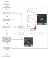 |
Fig. 1. Flowchart illustrating the visual identification of edges. An example of a galaxy, SDSS J003143.28+005402.4, and its profiles with the identified edge (vertical dotted line) is shown in the top right side of the flowchart. If the galaxy is symmetric, the relevant parameters in the edge, namely, Redge, the colour and mass density at the edge are saved. However, if the galaxy contains any non-symmetric features such as tidal streams in its outskirts such as the example SDSS J012859.56−003342.96 shown in the lower section of the flowchart, they are masked and the process of finding the edge is attempted once again. No edges are reported for cases when even an improvement in the masking did not present an edge. See Sect. 5.1 for details. |
In the case of the colour profile, the criteria we used as a signature of the edge depended on the morphology of the galaxy. For disk galaxies, we searched for the location of a sudden reddening in the outer part of the profile, indicative of the end of the star-forming disk (Sect. 5.2). For elliptical galaxies, we used the location of a sudden transition towards bluer g − r colours in the profile, potentially related to an outer envelope which assembled more recently compared to the galaxy’s (redder) central regions (Sect. 5.3). And for dwarf galaxies, the signature of the edge in the colour profile appeared either as a transition to bluer or redder outskirts, a reflection of the varied star formation histories possible in these galaxies (inside-out or outside-in, respectively). We show examples of all three morphological types in the sub-sections below.
Once an initial identification of the edge is made using the above criteria, we plotted an ellipse (the same used to derive the radial profiles) at Redge on the galaxy image to check whether the outskirts of the galaxy are elliptically symmetric in 2D. We show an example in the top right side of the flowchart of a galaxy and the profiles with the identified edge. If the galaxy is symmetric, we saved all the relevant parameters in the edge, namely, Redge, the colour and mass density at the edge.
If a galaxy did not show a similar feature in its profile as shown in the example or is not symmetric in the outskirts, we further examined the 2D image for contaminants such as bright stars, neighbouring galaxies or streams that could affect the structure of the profile if the automated masking did not adequately remove the contaminated regions in the image. We also show an example in the lower section of the flowchart of a galaxy that contains tidal-like features beyond the edge. The profiles of this particular galaxy and other difficult cases are shown in Appendix A. We then re-computed the radial profiles for the galaxy and re-examined the data to locate an edge. We do not report edges in cases where even an improvement in masking and profile derivation did not allow us to locate an edge in our analysis (37% of our full sample; details in the next section.).
Following the procedure detailed above, the edge for each galaxy was identified by the authors N. Chamba (NC) and I. Trujillo (IT). To quantify any dispersion in our inspections, we repeated our identifications and computed the average difference between these measurements. This quantity provides an estimate of the uncertainty in the visualisation of the edge.
We also show that our criteria and measurements are independent of the depth of the imaging used in Appendix B. The analysis is divided in two parts. In Appendix B.1, we examine a nearby (13.5 Mpc; Monelli & Trujillo 2019) disk galaxy with an edge, NGC1042, using deeper imaging from the LBT Imaging of Galactic Haloes and Tidal Structures (LIGHTS) Survey (Trujillo et al. 2021). We show that while deeper imaging allows one to characterise the edge with a higher signal-to-noise ratio, the edge of this galaxy may still be located with IAC Stripe 82 depth following our visualisation procedure. In Appendix B.2, we compare the surface brightness at which the edges of our parent sample appear with the limiting surface brightness of the IAC Stripe 82 images used. We show that all the edges studied in this work appear at surface brightnesses above the limiting depth of our data.
5.2. Dependence on orientation: Late-type galaxies
In the models studied by Martín-Navarro et al. (2014), the edge of a low-inclination Milky-Way-like galaxy with a bulge, disk and stellar halo appears as a very soft bump (or shallow change in slope) in the outer surface brightness profile while that of an edge-on galaxy of equal stellar mass appears prominently as a sharper cutoff. To complement this finding and visualise our definition of the edge, we show a few best case examples from our galaxy sample in Fig. 2 and how the appearance of the edge of a galaxy changes with orientation for real late-type galaxies with similar (inclination corrected) rotational velocities (see Sect. 3). For each galaxy, we show the IAC Stripe 82 gri-colour composite image with a pink contour marking the identified edge, g, r, GALEX NUV and FUV surface brightness profiles, g − r colour profile and resulting stellar mass density profile, Σ⋆. The location of the edge is also marked in the panels as a dotted, grey vertical line.
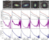 |
Fig. 2. Edges of galaxies as viewed in edge-on (left) to face-on (right) orientations. The galaxies were selected to have similar rotational velocities Vrot ∼ 145 km s−1. Left to right: IAC Stripe 82 gri-colour composite image overlaid on a grey scaled gri-band summed image for contrast, surface brightness profiles in the SDSS g, r, GALEX NUV and FUV bands, g − r colour profile and the corresponding Σ⋆ stellar mass density profile. The pink contour in the gri-image and the vertical dotted lines in the other panels indicate the edge of the galaxy. |
Figure 2 shows that edges appear at the location where there is a change in slope in the outer part of the surface brightness profiles (mainly in the UV). This location corresponds to the region where the g − r colour rapidly becomes redder. The U-shape of colour profiles in disk galaxies were firstly identified in Bakos et al. (2008) and Azzollini et al. (2008). This sudden reddening in the outer part of the colour profile is indicative of both the significant drop in in situ star formation (as also confirmed by the truncation in the UV) and the emergence of the stellar halo component and/or stars migrated from the star-forming regions in the disk to the outskirts. We made use of this feature collectively as the criteria to identify the edge in the rest of our late-type, spiral galaxy sample.
The radial profiles of galaxies have been derived using elliptical annuli (Sect. 4). In Appendix C, we confirm that this method does not hinder our ability to identify the edges of low-inclination galaxies using their radial profiles compared to the method adopted for edge-on galaxies, that is to say using a slit through the galaxy’s semi-major axis (see e.g., Martínez-Lombilla et al. 2019). We compare the ellipse and slit method for two galaxies: an edge-on case (UGC 09138) and a low-inclination one (NGC 1042) to study the effect of both these methods on galaxy orientation. We show that for UGC 09138, the elliptical annuli technique makes it unfeasible to locate the edge while for NGC 1042 the location of the edge is possible with either method. Therefore, our identification of the edge for low-inclination galaxies is not hampered by the method we adopted to derive their radial profiles. We illustrate and explain the criteria we used to identify the edges of the elliptical and dwarf galaxies in our sample in the sections below.
5.3. The edges of early-type galaxies
Contrary to what happens in galaxies undergoing star formation, in the case of elliptical galaxies in our sample, their g − r radial profiles follow a similar global shape as shown in Fig. 3. The galaxies shown have a similar stellar mass ∼1011.5 M⊙. To locate their edges we have used a drastic change (a factor of five or higher difference in slope before and after the edge in the cases shown here) in colour in the outer parts of the system to mark a difference between the bulk of the object (with an homogeneous red colour) and potentially infalling (bluer) new material. Upon making this choice to mark the edge of these galaxies, we are implicitly assuming that the bulk of the elliptical galaxy was formed in an early burst and that the colour transition to the blue indicates the transition from the location of the original star formation radius to the outer envelope which was assembled (relatively) more recently.
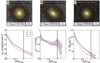 |
Fig. 3. Three examples of elliptical galaxies from the parent sample with stellar mass ∼1011 M⊙. Top: gri-band colour composite images, overlaid on the background gri summed image in grey scale, of the galaxies denoted as A (left), B (middle) and C (right). The SDSS J2000 identifier and Redge are labelled for these galaxies as in Fig. 2. Bottom, left to right: the μg, g − r and Σ⋆ profiles of the objects. The edges for these galaxies are visible as a sudden transition from red to blue in their g − r colour profiles (see Sect. 5.3 for details). The locations of the edges occur at mass densities Σ⋆(Redge) > 1 M⊙ pc−2. |
5.4. The edges of dwarf galaxies
For the dwarf galaxies in Fig. 4, we find that the edge is visible in their g − r profiles and/or stellar mass density profile. These galaxies have a stellar mass ∼108 M⊙, and were chosen to illustrate the diversity in the colour radial profiles of dwarf galaxies which reflect their different morphology and substructure (see also the work by Herrmann et al. 2016). According to HyperLeda6 (Makarov et al. 2014), the morphology of these galaxies from case A to C labelled in the figure are Irr, Sd and SABd respectively. The x-axis of the radial profiles are scaled to the location of Redge and the located edge is marked with the vertical black line. The edges of these galaxies occur at mass densities Σ⋆(Redge)≲2 M⊙ pc−2. For clarity, we additionally explored case A using the semi-major axis method in Appendix C.1, confirming the Redge identified as a change in slope in the radial profiles. In case B and C particularly, the edge marks the transition towards either bluer or redder outskirts. This observation could be related to inside-out or outside-in star formation in the dwarfs (e.g., Zhang et al. 2012). In a future paper, we explore the connection between the transition to redder or bluer outskirts in dwarf galaxies and galaxy environment (Chamba & Hayes, in prep.).
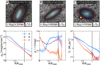 |
Fig. 4. Similar to Fig. 3, but for three dwarf galaxies with stellar mass ∼108 M⋆. These examples were specifically chosen to illustrate the diversity in the colour profiles of this galaxy population and the criteria we use to we locate the edge in these different cases. In case A, we use the change in slope in the Σ⋆ profile. In B and C, the edge is identified as a sudden transition to bluer colours in the g − r profile (see Sect. 5.4 for details). The edges of these galaxies occur at mass densities Σ⋆(Redge)≲2 M⊙ pc−2. |
We identified the edges of the spirals, ellipticals and dwarfs in the rest of our sample following the physically motivated criteria described above. In summary, the signature of the edge of a galaxy may be identified as: a change in slope or cutoff in the radial surface brightness and/or stellar mass density profile (Sect. 2), a sudden reddening in the outer part of the colour profile for spiral galaxies, indicative of the end of the star-forming disk (Sect. 5.2), a sudden transition from red to blue colours for elliptical galaxies, to mark a difference between the core and recent infalling material, respectively (Sect. 5.3), or any of the above for dwarf galaxies. A transition to bluer or redder outskirts could reflect the inside-out or outside-in formation history, respectively (Sect. 5.4). We leave the exploration of alternative criteria to mark the edges of galaxies for future work using deeper and/or higher resolution data.
6. Results
Using the above procedure, we identified edges in 171 (or 61.2% of the) ellipticals, 273 (58.8% of) spirals and 180 (68.7% of) dwarfs (i.e 624 or 62% of the galaxies in total) in our parent sample and 21 galaxies in the collective B12 and P17 samples. The 381 galaxies with no identified edges in our parent sample comprise of 107 ellipticals, 190 spirals and 84 dwarfs. Eighty-seven galaxies within this sub-sample were removed due to heavy contamination from bright stars, neighbouring galaxies and clouds of Galactic cirrus. Such highly contaminated galaxies may be studied with ad-hoc techniques but this is beyond the scope of the analysis and pipelines we developed for this work. Further investigation reveals that the majority of galaxies without identified edges have very low inclination (mean axis-ratio of q = 0.71), 84% of which have q > 0.5. This finding is expected given the difficulty in identifying edges in low-inclination galaxies (see Fig. 2).
Figure 5 shows the main result of this work: the Redge-stellar mass plane (left panels) and the Σ⋆(Redge)-stellar mass plane (right panels) for the parent sample. Each row shows the data points in both planes labelled according to each galaxy’s morphology, colour and age at the edge. The latter relations are similar when the total magnitudes of the galaxy in g and r are used to compute the colour and age. Our results also do not change if we compute the age with a fixed metallicity [M/H] of 0 or −0.71 (see Sect. 4). For clarity, we show our measurements for the nearby B12 and P17 galaxies separately in Fig. 6.
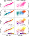 |
Fig. 5. Redge–stellar mass (left) and Σ⋆(Redge)–stellar mass (right) relations derived in this work. Only those galaxies where an edge was identified are plotted (624 objects). The grey lines in the Redge–stellar mass planes are lines of constant stellar mass surface density within the Redge of the object. Top to bottom: each row shows the same observed relations (top), colour coded according to the morphology of the galaxies, (g − r)edge and a proxy for the age at Redge, for a fixed metallicity [M/H]= − 0.71. We plot the uncertainties in our measurements (see Sect. 4) only in the second row for clarity in the other panels. |
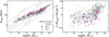 |
Fig. 6. Similar to Fig. 5, now including the measurements in this work for the sample of galaxies studied in B12 and P17. The grey circles are the measurements for our sample. |
Following Trujillo et al. (2020) and Chamba et al. (2020), we obtain the best fit slopes and dispersion values for the scaling relations using a Huber Regressor (Huber 1964) which is a linear regression model robust to outliers. The global Redge–stellar mass plane follows a power law of the form  where β = 0.31 ± 0.01 and the relation has an observed dispersion of σRedge = 0.10 ± 0.01 dex. For the individual galaxy populations, β is 0.54 ± 0.03 for the elliptical galaxies (E0–S0+), 0.27 ± 0.02 for spirals (S0/a–Im) and 0.32 ± 0.03 for the dwarfs. If we remove the uncertainty from our visual identification of Redge (σvis ∼ 0.04 dex) which we computed using NC and IT’s repeated measurements (see Sect 5.1) from σRedge in quadrature, we achieve a scatter of the relation
  dex. These values are provided in Table 1.
Best-fit parameters for the Redge-stellar mass relation.
The above dispersion values also include observational errors due to background and stellar mass estimation. We find comparable values to the uncertainty in stellar mass in our galaxy sample to that published in Trujillo et al. (2020; i.e. 0.047 dex) and the effect of the background estimation on the location of Redge amounts to 0.072 dex in our full sample. We may use these estimations of the uncertainty to compute the global intrinsic scatter of the size–stellar mass relation. Removing these values from σRedge in quadrature gives an intrinsic scatter of 0.059 dex. If we include the result of our visual identification of Redge (σvis ∼ 0.04 dex) the intrinsic scatter is 0.043 dex (but see Stone et al. 2021, for a detailed treatment of observational errors on the scatter of galaxy scaling relations).
In the case of the Σ⋆(Redge)–stellar mass plane, we obtained two linear fits to describe the data by separating the sample in two intervals at log[M⋆/M⊙] ∼ 10.5, in other words interval I1 where log[M⋆/M⊙]< 10.5 and I2 where log[M⋆/M⊙] ≥ 10.5. We split our sample in this fashion because 1) a single polynomial fit to the data performed very poorly and 2) spiral galaxies are over represented in our sample (274 objects out of the 624 galaxies with identified edges). Therefore, by splitting the sample at a stellar mass of log[M⋆/M⊙] ∼ 10.5, the two intervals I1 and I2 are more comparable in terms of sample size (294 and 330 galaxies, respectively) and it is also the location where the slope of the Σ⋆(Redge)–stellar mass relation increases. We plot these results explicitly in Appendix D. The two linear fits may be used to determine the average location of the edge (in mass density) ⟨Σedge(M⋆)⟩, as a function of galaxy stellar mass, given by:
![$$ \begin{aligned}&\log [\left\langle \Sigma _{\rm edge}(M_{\star })\right\rangle ] = 0.13\log \left[\frac{M_{\star }}{M_{\odot }} \right] - 1.32 (\log \left[\frac{M_{\star }}{M_{\odot }} \right]< 10.5)\end{aligned} $$](/articles/aa/full_html/2022/11/aa43612-22/aa43612-22-eq7.gif)
![$$ \begin{aligned}&\log [\left\langle \Sigma _{\rm edge}(M_{\star })\right\rangle ] = 0.39\log \left[\frac{M_{\star }}{M_{\odot }} \right] - 3.97 (\log \left[\frac{M_{\star }}{M_{\odot }} \right]\ge 10.5). \end{aligned} $$](/articles/aa/full_html/2022/11/aa43612-22/aa43612-22-eq8.gif)
The uncertainties in the slopes βI1 = 0.13 ± 0.03 and βI2 = 0.39 ± 0.06 and the dispersion in both relations are similar: σI1 = 0.29 ± 0.02 dex and σI2 = 0.28 ± 0.02 dex.
We plot the distributions in Redge and Σedge as histograms in Fig. 7 for each morphological group studied here (upper panels) and we use the linear fits to the Redge– and Σ⋆(Redge)–stellar mass planes to highlight the stratification in (g − r)edge colour in those relations (lower panels). The subscript ‘fit’ in this figure refers to the best fit line for each plane, which is the line that describes the average value of Redge and Σ⋆(Redge) at each stellar mass.
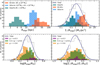 |
Fig. 7. Representation of the results shown in Fig. 5 as histograms. Top: the distribution of Redge (left) and Σ⋆(Redge). Bottom: the distribution of (g − r)edge in the Redge–stellar mass (left) and Σ⋆(Redge)–stellar mass (right) relations. The subscript ‘fit’ refers to the best fit line of each plane. |
The main features of the results shown in the above figures are described in the following. Galaxies where M⋆ ≲ 1011 M⊙ closely follow a power law of the form  and is comparable to the global slope of the size–stellar mass relation. We additionally fit our data to a relation with a fixed slope of 1/3, restricting the sample only to spiral galaxies or to both spiral and dwarf galaxies, finding that the y-intercept using both sub-samples did not change. This result supports the idea that both populations lie on the same slope.
We also observe a tilt in the Redge–stellar mass plane when M⋆ > 1011 M⊙. Massive elliptical galaxies dominate the scaling relation in this regime. At the same time, the mass density at the location of the edge depends on the total stellar mass of the galaxy with an up turn at log[M⋆/M⊙] ∼ 10.5. The slope of the Σ⋆(Redge)–stellar mass plane triples at this stellar mass.
In morphology, the average mass density at the location of the edge is 2.9 ± 0.1 M⊙ pc−2 for the E0-S0+ sample, 1.1 ± 0.04 M⊙ pc−2 for S0/a-Im and 0.6 ± 0.03 M⊙ pc−2 for the dwarfs. In other words, the density is lower for dwarfs by almost a factor of five and two compared to the massive ellipticals and spirals, respectively.
The colour (age) gradient at fixed stellar mass with Redge shows that larger galaxies have bluer (younger) edges. The observed colour gradient also produces a gradient in mass density at the location of the edge at fixed stellar mass where bluer edges are located in regions of lower mass densities. More specifically, for galaxies within a stellar mass range of 1010 − 1011 M⊙, we observe an age increase from ∼2 Gyr to ∼12 Gyr at the extreme ends of the scaling relation in Redge as the size of the galaxy decreases, assuming a fixed metallicity of [M/H]= − 0.71.
On average, galaxies located in the upper half of both the Redge– and Σ⋆(Redge)–stellar mass relations have bluer edges compared to the lower half. In Appendix B.2 we show that this observation is not a bias due to image depth or the limiting surface brightness of our data.
The B12 and P17 galaxies lie in the upper half of the Redge–stellar mass relation and in the lower regions of the Σ⋆(Redge)–stellar mass relation. This is consistent with the fact that the majority of the galaxies in these samples have been classified with Sb, Sc or later morphology. We plot the Redge– and Σ⋆(Redge)–stellar mass relations only for the late-type galaxies in our sample in Fig. 8 to highlight this statement.
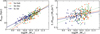 |
Fig. 8. Stratification of late-type galaxies in the Redge–stellar mass (left) and Σ⋆(Redge)–stellar mass (right) relation. The galaxies are grouped morphologically following Trujillo et al. (2020). The lines are the best-fit relations for each group in both panels. See text for details. |
7. Discussion
We have visually identified the edges of a large sample of ∼1000 low-inclination galaxies spanning a wide morphology (from dwarfs to ellipticals) and stellar mass range (107 M⊙ < M⋆ < 1012 M⊙). Sixty-two percent of the galaxies in our total sample presented identifiable edges following our visualisation procedure. We estimated the stellar mass density at their edge and then presented the resulting Redge– and Σ⋆(Redge)–stellar mass relations for these galaxies.
Our main results are discussed in the following sub-sections. We leave the exploration of how our work may be used in future large-scale catalogues in Appendix E. We find that the Σ⋆(Redge)–stellar mass relations in Eqs. (3) and (4) could be used to obtain the location of the edge and provide a proxy for the size of any galaxy, provided its stellar mass is known. These laws may be useful for larger galaxy samples and automated cataloguing in future multi-band surveys such as Rubin Observatory’s Legacy Survey of Space and Time (LSST).
7.1. The global slope of size–stellar mass relation: 
If we focus on the spirals and dwarfs in our study, we have found that these galaxy populations have Redge–stellar mass relations with comparable slopes (β ∼ 0.3 and close to a global slope ∼1/3; see Table 1), with an intrinsic dispersion ≲0.06 dex. These parameters are compatible with those obtained in Trujillo et al. (2020) using R1 (the fixed isomass contour at 1 M⊙ pc−2) for size. The global slope of 1/3 is observed over four orders of magnitudes in stellar mass 107 M⊙ < M⋆ < 1011 M⊙ in the size–stellar mass relation, despite the different stellar mass surface densities we measured at the edges of galaxies in this regime. The lower density we measure at the edge for dwarfs (∼0.6 M⊙ pc−2) compared to the spirals (∼1 M⊙ pc−2) could be reflective of the low star formation efficiency that has been observed in these galaxies (e.g., Leroy et al. 2008; Huang et al. 2012). However, despite this difference, the constant slope could imply that the dwarfs and spiral galaxies in our sample share a common mechanism by which in situ star formation may have occurred. This idea is not incompatible with the fact that several similarities in the structure of surface brightness, colour and stellar mass density profiles of dwarfs and spiral galaxies have been found in the literature within the context of galaxy outskirts (e.g., Hunter et al. 2011; Herrmann et al. 2016).
We contrast this result with those obtained using the effective radius (Re; de Vaucouleurs 1948), a popular measure for galaxy size in the literature and with which the resulting size–stellar mass plane has very different characteristics. The relation is more broken for different galaxy morphologies (see e.g., Shen et al. 2003; Brodie et al. 2011) and the dispersion is almost three times larger than that of the Redge–stellar mass plane (see also Trujillo et al. 2020). The broken scaling relations shown in these previous studies using Re have traditionally been interpreted to reflect different size formation or evolution mechanisms for the galaxies. From this perspective, the global slope representing an unbroken size–stellar mass relation found here does not obviously favour such interpretations and works to readdress these issues are currently ongoing. However, to give the reader a view on how extended the galaxies in our sample are compared to what Re suggests, we plot the ratios Redge/Re and R1/Re as a function of the respective sizes in Fig. 9. We compute Re in a model independent way using the growth curve of the galaxy in the g-band which is our deepest dataset. The R1 values were taken from Trujillo et al. (2020).
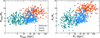 |
Fig. 9. Ratios Redge/Re (left) and R1/Re (right) as a function of the respective sizes for the labelled morphologies. The diagrams reinforce how extended galaxies are compared to what the effective radius represents Re. |
Particularly in Redge, it is clear for each galaxy type that while there is a change in Redge over tens of kiloparsecs (for example from 10 to 50 kpc for spirals), the ratio with Re is small (about 3–4). These results further support the need to rethink the concept of galaxy size and readdress the origin of the size–stellar mass relation (Chamba 2020).
7.2. Comparison between Redge and the isomass contour at 1 M⊙ pc−2
To further address the structure we have observed in the size–stellar mass relation (stratification and slopes), it is worth exploring how similar Redge is compared to R1. As mentioned in the Introduction, we studied the R1–stellar mass relation in Trujillo et al. (2020) and Chamba et al. (2020) because the isomass contour at 1 M⊙ pc−2 is physically motivated for Milky-Way-like galaxies as it is related to a star formation threshold. A fixed isomass contour at 1 M⊙ pc−2 is also easier to measure7 and reproduce which makes it more robust. For the sample of galaxies analysed here, we find that R1 appears at a similar surface brightness to Redge: on average R1 appears at μg = 27.4 ± 0.05 mag arcsec−2 in g (the standard deviation of this distribution is 1.2 mag) and Redge can be 0.4 ± 0.02 mag arcsec−2 brighter on average. Figure 10 shows Redge vs. R1, colour coded according to the galaxy’s stellar mass (top) and morphology (middle). The lower panel shows the histogram of the distribution in the Redge–R1 plane, with the sample divided according to their labelled morphology. The scatter in the Redge vs. R1 distribution is 0.088 dex with the elliptical (dwarf) galaxy population having smaller (slightly larger) Redge than R1 by ∼0.1 dex (0.05 dex) on average. Given these results, we recommend the use of R1 for galaxies of similar properties as those studied here if the measurement of Redge is not possible due to, for instance, poor signal-to-noise ratios.
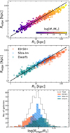 |
Fig. 10. Comparison between Redge and R1. The top and middle panels show Redge vs. R1 for the galaxies in our sample, colour coded in stellar mass and morphology, respectively. The solid black line in the upper panels is the one-to-one relation. The lower panel shows the same distribution as a histogram. |
This result allows us to explore the R1 of galaxies where we did not identify the presence of an edge. In Fig. 11 we plot the R1 of these galaxies (381 galaxes; 37% of the total sample) on the Redge–stellar mass plane. The majority of these galaxies have very low inclinations or are heavily contaminated in their outskirts (see Sect. 6). We see that the R1 of these galaxies follow the overall distribution of Redge in the size–mass plane within the uncertainties of our Redge measurements. The most visible deviation occurs at the higher mass end (M⋆ > 1011 M⊙), however, this can be explained by the fact that the majority of our elliptical galaxies have Redge at surface densities > 1 M⊙ pc−2 and thus results in smaller sizes (below the black points). In contrast, the R1 of all of the dwarf galaxies shown here appear to be within the distribution of Redge, even though Redge of the dwarfs are on average slightly larger (lower panel of Fig. 10). Therefore, from Fig. 11 we may conclude that the exclusion of these galaxies without identified edges from our work does not bias our analysis and the main results discussed in this section remain unchanged. However, we note that the scatter using R1 is smaller compared to Redge because of the difficulty in measuring the edge compared to a fixed isomass contour.
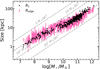 |
Fig. 11. R1 of galaxies where we were unable to locate the presence of edges (black) over plotted on the Redge–stellar mass plane (pink). |
7.3. The tilt in the Redge– and Σ⋆(Redge)–stellar mass planes
The comparison between Redge and R1 above shows that the two measures deviate from the one-to-one relation (solid black line in Fig. 10) for the majority of the higher mass elliptical galaxies in our sample (especially when M⋆ > 1011 M⊙), with Redge < R1. Consequently, Redge appears at stellar mass densities > 1 M⊙ pc−2 (∼3 M⊙ pc−2 on average) for these galaxies and can be seen as a tilt in the Redge– and Σ⋆(Redge)–stellar mass relations (Fig. 5). A similar tilt was observed in the R1–stellar mass plane in Trujillo et al. (2020), however, here we have additionally found that the edges of these galaxies have older stellar populations than the late-types (g − r colour > 0.6). The tilt observed here (characterised by the slope of the size–stellar mass plane) is two times steeper for the ellipticals than the spirals and could be additional evidence towards a major difference in the mechanisms responsible for size growth between these two morphological groups, such as accretion which predominantly occurs in the most massive galaxies.
To understand why the star formation threshold for elliptical galaxies is higher than for spiral galaxies, we need to consider the epoch at which these massive galaxies initially formed their stars. As pointed out in Trujillo et al. (2020), it has been observed that massive elliptical galaxies had bursty star formation histories at high redshift with star formation rates as extreme as 1000 M⊙ yr−1 (e.g., Riechers et al. 2013; Jaskot et al. 2015). A high rate of star formation could provide a large enough energy budget to the surrounding gas, making it difficult for stars to form preferentially at low surface densities by increasing the galaxy’s star formation threshold. Therefore, the edges of these massive galaxies could be tracing star formation that occurred during an epoch of high star formation rate which formed the core (bulge) material of the galaxy. Notice that M⋆ > 1011 M⊙ is also the regime where pressure supported systems could be dominating the scaling relation compared to rotationally supported galaxies (see Emsellem et al. 2011). This difference (as well as in symmetry, considering spherical vs. disk) between these galaxies could have consequences on the density at which stars would have preferentially formed in galaxies in the early Universe.
We have selected a specific criterion to locate the edges of elliptical galaxies: a sudden colour transition from red to blue (Sect. 5.3) and we have left the exploration of alternative criteria for future work. However, based on our results it is interesting to consider that deviations from the global slope in the size–stellar mass relation  could indicate deviations from the early star formation phase in the core component of these galaxies. If we fix the most massive galaxies with M⋆ > 1011.5 M⊙ (i.e. where only elliptical galaxies in our sample deviate from the global slope) to lie on the
  relation, we obtain that their Redge would be on average almost ∼20 kpc smaller. Consequently, the stellar mass density at these locations is more than double compared to that of the identified edges for these galaxies (i.e ∼8 M⊙ pc−2 on average). Such a threshold would enclose the bulk of the stellar component in relic galaxies, which are those galaxies that represent the core component of the majority of elliptical galaxies in the nearby Universe (e.g., NGC 1277; Trujillo et al. 2014). This alternative criterion would also better represent the visual edge of case C shown in Fig. 3. With either this new criterion or that adopted in our identification procedure (Sect. 5.1), if the edges indicate a star formation threshold, our conclusion that the edges of elliptical galaxies occur at higher stellar mass densities remains unchanged.
7.4. The stratification of late-types
A stratification of late-type galaxies in morphology was previously found by Saintonge & Spekkens (2011) and Trujillo et al. (2020) using R23.5 (the isophote at 23.5 mag arcsec−2 in the SDSS i-band) and R1 respectively, with its origin still unknown. However, with Redge we have found that while the average stellar mass density at the star formation threshold for these galaxies is 1 M⊙ pc−2, there appears to be an additional variation in their stellar population properties where larger galaxies have bluer edges (Figs. 5, 6 and 8).
The stratification in size and colour suggests that larger galaxies may have reached their current size at a later time than smaller ones. This interpretation follows from the assumption that bluer colours trace ongoing or recent star formation while redder colours reflect the presence of older stellar material. For galaxies within the 1010 − 1011 M⊙ stellar mass range studied here, outskirts that are populated with young to intermediate aged stars (< 6 Gyr) are possible due to, for example, the accretion of gas-rich satellite galaxies that trigger new star formation (e.g., Grand et al. 2017), the galaxy’s enriched H I content (e.g., Kauffmann 2015) or the migration of stars from the disk to the outskirts (e.g., Roškar et al. 2008). Of course the latter scenario could also result in redder outskirts with older stars but star formation may still occur in these regions (see the review by Elmegreen & Hunter 2017).
The idea that larger late-type galaxies are generally younger8 is also not incompatible with the stratification we observe in their global morphology with Sa-Sab galaxies showing smaller sizes compared to Sc-Sd types (see Fig. 8). Sa-Sab galaxies generally have lower star formation rates (often in a path towards quenching) than Sc or other later types where they are much higher (e.g., González Delgado et al. 2016; Bait et al. 2017). Our data could be reflective of this difference between galaxy types. Additionally, the lower half of the size–stellar mass relation is populated by elliptical galaxies of similar stellar mass (see Fig. 5). Elliptical galaxies are generally red, old and quiescent. From this perspective, the stratification we observe could be connected to when galaxies reached their present day stellar mass. In other words, a stratification between the ‘newer’ late-type spirals and the ‘older’ early-type elliptical galaxies (see also the recent work by Watkins et al. 2022).
The interpretation of whether a stratification in morphology exists in the lower mass dwarf regime is likely subjected to incompleteness effects (due to the limit in magnitude selected for spectroscopic targets in SDSS; see the discussion in Chamba et al. 2020). However, at least from the lower panels of Fig. 7, there appears to be a stratification of galaxy size in colour where all of the blue edged dwarf galaxies (g − r ≲ 0.3) appear in the upper half of the size–stellar mass relation. We do not possess morphological information of these galaxies in our sample to investigate this here further and leave it for future work.
8. Conclusions
We have identified the edges of one of the largest samples of low-inclination galaxies. Our work expands on a physically motivated approach to define the edges (and consequently the sizes) of galaxies as the outermost location where in situ star formation (either ongoing or in the past) significantly drops within these systems. This idea is based on the gas density threshold required for the star formation process in galaxies (e.g., Schaye 2004). Our main conclusions can be summarised as follows:
-
The size–stellar mass relation using Redge has a global slope of ∼1/3 and an intrinsic scatter ≲0.06 dex over a wide stellar mass range 107 M⊙ < M⋆ < 1012 M⊙ suggesting a common mechanism of in situ star formation. The structure of the relation is similar to that using R1 (see Trujillo et al. 2020; Chamba et al. 2020).
-
Massive elliptical galaxies dominate the scaling relation when M⋆ ≳ 1011 M⊙. This region corresponds to the tilt in the Redge– and Σ⋆(Redge)–stellar mass planes where the slope of the size–stellar mass relation doubles, potentially tracing the different epoch and high efficiency at which massive galaxies formed their stars.
-
The stellar mass surface density at the edge (and consequently the star formation threshold) is a function of stellar mass and depends on the morphology of galaxies: it averages to ∼3 M⊙ pc−2 (or higher) for ellipticals, ∼1 M⊙ pc−2 for spirals and ∼0.6 M⊙ pc−2 for dwarfs.
-
Redge is larger for bluer (i.e. younger) galaxies at a fixed stellar mass, reflective of when these galaxies reached their present-day size.
Given that Redge is very similar to the location of the 1 M⊙ pc−2 isomass contour (R1) for the majority of the galaxies, we recommend the use of the latter (or a higher isomass contour for elliptical galaxies) when the measurement of Redge is challenging, for example due to imaging with low signal-to-noise. Due to the low scatter and physical significance underlying our measurements, we propose our size definition to be used in future deep, large-scale catalogues such as those from the LSST, to reach extreme galaxies of low surface brightness or high redshift galaxies with JWST and shift our understanding of how galaxies truly grow in size.
Values obtained from the HyperLeda database (Makarov et al. 2014): http://leda.univ-lyon1.fr/
R1 can be measured provided that the data is sufficiently deep, for example deeper than SDSS for low-inclination galaxies; see Fig. 6 in Trujillo et al. (2021).
A slightly different approach to this method is the use of a wedge shape (see Stone et al. 2021).
Acknowledgments
We thank the anonymous referee for their detailed comments which helped to significantly improve the clarity of this manuscript. We acknowledge financial support from the State Research Agency (AEI-MCINN) of the Spanish Ministry of Science and Innovation under the grant ‘The structure and evolution of galaxies and their central regions’ with reference PID2019-105602GB-I00/10.13039/501100011033 and grant PID2019-107427GB-C32, and from IAC projects P/300624 and P/300724, financed by the Ministry of Science and Innovation, through the State Budget and by the Canary Islands Department of Economy, Knowledge and Employment, through the Regional Budget of the Autonomous Community. N.C. acknowledges support from the research project grant ‘Understanding the Dynamic Universe’ funded by the Knut and Alice Wallenberg Foundation under Dnr KAW 2018.0067 and thanks Matthew Hayes, Fernando Buitrago, Claudio Dalla Vecchia, Aura Obreja, L. Pascho, and Naomi Samsoodeen for interesting discussions. J.H.K. and I.T.C. acknowledge support from the ACIISI, Consejería de Economía, Conocimiento y Empleo del Gobierno de Canarias and the European Regional Development Fund (ERDF) under grant with reference PROID2021010044. Funding for the Sloan Digital Sky Survey IV has been provided by the Alfred P. Sloan Foundation, the U.S. Department of Energy Office of Science, and the Participating Institutions. SDSS-IV acknowledges support and resources from the Center for High-Performance Computing at the University of Utah. The SDSS web site is www.sdss.org. SDSS-IV is managed by the Astrophysical Research Consortium for the Participating Institutions of the SDSS Collaboration including the Brazilian Participation Group, the Carnegie Institution for Science, Carnegie Mellon University, the Chilean Participation Group, the French Participation Group, Harvard-Smithsonian Center for Astrophysics, Instituto de Astrofísica de Canarias, The Johns Hopkins University, Kavli Institute for the Physics and Mathematics of the Universe (IPMU)/University of Tokyo, the Korean Participation Group, Lawrence Berkeley National Laboratory, Leibniz Institut für Astrophysik Potsdam (AIP), Max-Planck-Institut für Astronomie (MPIA Heidelberg), Max-Planck-Institut für Astrophysik (MPA Garching), Max-Planck-Institut für Extraterrestrische Physik (MPE), National Astronomical Observatories of China, New Mexico State University, New York University, University of Notre Dame, Observatário Nacional/MCTI, The Ohio State University, Pennsylvania State University, Shanghai Astronomical Observatory, United Kingdom Participation Group, Universidad Nacional Autónoma de México, University of Arizona, University of Colorado Boulder, University of Oxford, University of Portsmouth, University of Utah, University of Virginia, University of Washington, University of Wisconsin, Vanderbilt University, and Yale University. This research has made use of the NASA/IPAC Extragalactic Database (NED), which is operated by the Jet Propulsion Laboratory, California Institute of Technology, under contract with the National Aeronautics and Space Administration. We acknowledge the usage of the HyperLeda database http://leda.univ-lyon1.fr This work was partly done using GNU Astronomy Utilities (Gnuastro, ascl.net/1801.009) version 0.14. Work on Gnuastro has been funded by the Japanese Ministry of Education, Culture, Sports, Science, and Technology (MEXT) scholarship and its Grant-in-Aid for Scientific Research (21244012, 24253003), the European Research Council (ERC) advanced grant 339659-MUSICOS, European Union’s Horizon 2020 research and innovation programme under Marie Sklodowska-Curie grant agreement No 721463 to the SUNDIAL ITN, and from the Spanish Ministry of Economy and Competitiveness (MINECO) under grant number AYA2016-76219-P. Software: Astropy, (http://www.astropy.org) a community-developed core Python package for Astronomy (Robitaille et al. 2013; Price-Whelan et al. 2018); Gnuastro (astwarp; Akhlaghi & Ichikawa 2015); IMFIT (Erwin 2015); Jupyter Notebooks (Kluyver et al. 2016); Matplotlib (Hunter 2007); MTObjects (Teeninga et al. 2016; Haigh et al. 2021); NumPy (Oliphant 2006); doi:10.1109/MCSE.2011.37; SAO Image DS9 (Smithsonian Astrophysical Observatory 2000); SciPy (Jones et al. 2001); SWarp (Bertin 2010); and TOPCAT (Taylor 2005).
References
- Abazajian, K. N., Adelman-McCarthy, J. K., Agüeros, M. A., et al. 2009, ApJS, 182, 543 [Google Scholar]
- Akhlaghi, M., & Ichikawa, T. 2015, ApJS, 220, 1 [Google Scholar]
- Azzollini, R., Trujillo, I., & Beckman, J. E. 2008, ApJ, 679, L69 [NASA ADS] [CrossRef] [Google Scholar]
- Bait, O., Barway, S., & Wadadekar, Y. 2017, MNRAS, 471, 2687 [NASA ADS] [CrossRef] [Google Scholar]
- Bakos, J., & Trujillo, I. 2012, ArXiv e-prints [arXiv:1204.3082] [Google Scholar]
- Bakos, J., Trujillo, I., & Pohlen, M. 2008, ApJ, 683, L103 [NASA ADS] [CrossRef] [Google Scholar]
- Bertin, E. 2010, SWarp: Resampling and Co-adding FITS Images Together (Astrophysics Source Code Library) [Google Scholar]
- Brodie, J. P., Romanowsky, A. J., Strader, J., & Forbes, D. A. 2011, AJ, 142, 199 [NASA ADS] [CrossRef] [Google Scholar]
- Cardona-Barrero, S., Di Cintio, A., Battaglia, G., Macciò, A. V., & Taibi, S. 2022, ArXiv e-prints [arXiv:2206.10481] [Google Scholar]
- Chamba, N. 2020, Res. Notes Am. Astron. Soc., 4, 117 [NASA ADS] [Google Scholar]
- Chamba, N., Trujillo, I., & Knapen, J. H. 2020, A&A, 633, L3 [NASA ADS] [CrossRef] [EDP Sciences] [Google Scholar]
- Crnojević, D. 2017, in Outskirts of Galaxies, eds. J. H. Knapen, J. C. Lee, & A. Gil de Paz, Astrophys. Space Sci. Lib., 434, 31 [CrossRef] [Google Scholar]
- de Vaucouleurs, G. 1948, Annales d’Astrophysique, 11, 247 [NASA ADS] [Google Scholar]
- Díaz-García, S., Comerón, S., Courteau, S., et al. 2022, A&A, in press, https://doi.org/10.1051/0004-6361/202142447 [Google Scholar]
- Efstathiou, G., & Silk, J. 1983, Fund Cosmic. Phys., 9, 1 [Google Scholar]
- Elmegreen, B. G., & Hunter, D. A. 2017, Astrophys. Space Sci. Lib., 434, 115 [NASA ADS] [CrossRef] [Google Scholar]
- Emsellem, E., Cappellari, M., Krajnović, D., et al. 2011, MNRAS, 414, 888 [Google Scholar]
- Erwin, P. 2015, ApJ, 799, 226 [Google Scholar]
- Fall, S. M., & Efstathiou, G. 1980, MNRAS, 193, 189 [NASA ADS] [CrossRef] [Google Scholar]
- Fliri, J., & Trujillo, I. 2016, MNRAS, 456, 1359 [Google Scholar]
- Font, A. S., McCarthy, I. G., Poole-Mckenzie, R., et al. 2020, MNRAS, 498, 1765 [NASA ADS] [CrossRef] [Google Scholar]
- Gaia Collaboration (Brown, A. G. A., et al.) 2016, A&A, 595, A2 [NASA ADS] [CrossRef] [EDP Sciences] [Google Scholar]
- González Delgado, R. M., Cid Fernandes, R., Pérez, E., et al. 2016, A&A, 590, A44 [NASA ADS] [CrossRef] [EDP Sciences] [Google Scholar]
- Grand, R. J. J., Gómez, F. A., Marinacci, F., et al. 2017, MNRAS, 467, 179 [NASA ADS] [Google Scholar]
- Haigh, C., Chamba, N., Venhola, A., et al. 2021, A&A, 645, A107 [NASA ADS] [CrossRef] [EDP Sciences] [Google Scholar]
- Herrmann, K. A., Hunter, D. A., & Elmegreen, B. G. 2016, AJ, 151, 145 [NASA ADS] [CrossRef] [Google Scholar]
- Holmberg, E. 1958, Meddelanden fran Lunds Astronomiska Observatorium Serie II, 136, 1 [Google Scholar]
- Huang, S., Haynes, M. P., Giovanelli, R., & Brinchmann, J. 2012, ApJ, 756, 113 [Google Scholar]
- Huang, S., Leauthaud, A., Bradshaw, C., et al. 2022, MNRAS, 515, 4722 [NASA ADS] [CrossRef] [Google Scholar]
- Huber, P. J. 1964, Ann. Math. Stat., 35, 73 [CrossRef] [Google Scholar]
- Hunter, J. D. 2007, Comput. Sci. Eng., 9, 90 [NASA ADS] [CrossRef] [Google Scholar]
- Hunter, D. A., Elmegreen, B. G., Oh, S.-H., et al. 2011, AJ, 142, 121 [NASA ADS] [CrossRef] [Google Scholar]
- Infante-Sainz, R., Trujillo, I., & Román, J. 2020, MNRAS, 491, 5317 [Google Scholar]
- Jaskot, A. E., Oey, M. S., Salzer, J. J., et al. 2015, ApJ, 808, 66 [NASA ADS] [CrossRef] [Google Scholar]
- Jiang, L., Fan, X., Annis, J., et al. 2008, AJ, 135, 1057 [NASA ADS] [CrossRef] [Google Scholar]
- Jing, J., Liu, S., Wang, G., Zhang, W., & Sun, C. 2022, Neurocomputing, 503, 259 [CrossRef] [Google Scholar]
- Jones, E., Oliphant, T., Peterson, P., et al. 2001, SciPy: Open source scientific tools for Python, http://www.scipy.org/ [Google Scholar]
- Kauffmann, G. 2015, MNRAS, 450, 618 [NASA ADS] [CrossRef] [Google Scholar]
- Kennicutt, R. C., Jr 1989, ApJ, 344, 685 [CrossRef] [Google Scholar]
- Kluyver, T., Ragan-Kelley, B., Pérez, F., et al. 2016, in Positioning and Power in Academic Publishing: Players, Agents and Agendas, eds. F. Loizides, & B. Schmidt, (IOS Press), 87 [Google Scholar]
- Kniazev, A. Y., Grebel, E. K., Pustilnik, S. A., et al. 2004, AJ, 127, 704 [NASA ADS] [CrossRef] [Google Scholar]
- Leroy, A. K., Walter, F., Brinks, E., et al. 2008, AJ, 136, 2782 [Google Scholar]
- Makarov, D., Prugniel, P., Terekhova, N., Courtois, H., & Vauglin, I. 2014, A&A, 570, A13 [NASA ADS] [CrossRef] [EDP Sciences] [Google Scholar]
- Maraston, C., Pforr, J., Henriques, B. M., et al. 2013, MNRAS, 435, 2764 [NASA ADS] [CrossRef] [Google Scholar]
- Martin, D. C., Fanson, J., Schiminovich, D., et al. 2005, ApJ, 619, L1 [Google Scholar]
- Martín-Navarro, I., Trujillo, I., Knapen, J. H., Bakos, J., & Fliri, J. 2014, MNRAS, 441, 2809 [CrossRef] [Google Scholar]
- Martínez-Lombilla, C., Trujillo, I., & Knapen, J. H. 2019, MNRAS, 483, 664 [CrossRef] [Google Scholar]
- Monelli, M., & Trujillo, I. 2019, ApJ, 880, L11 [NASA ADS] [CrossRef] [Google Scholar]
- Morrissey, P., Conrow, T., Barlow, T. A., et al. 2007, ApJS, 173, 682 [Google Scholar]
- Nair, P. B., & Abraham, R. G. 2010, ApJS, 186, 427 [Google Scholar]
- Neumann, J., Thomas, D., Maraston, C., et al. 2021, MNRAS, 508, 4844 [NASA ADS] [CrossRef] [Google Scholar]
- Oliphant, T. 2006, NumPy: A guide to NumPy (USA: Trelgol Publishing) [Google Scholar]
- Peters, S. P. C., van der Kruit, P. C., Knapen, J. H., et al. 2017, MNRAS, 470, 427 [NASA ADS] [CrossRef] [Google Scholar]
- Price-Whelan, A., Sipőcz, B., Günther, H., et al. 2018, AJ, 156, 123 [NASA ADS] [CrossRef] [Google Scholar]
- Quirk, W. J. 1972, ApJ, 176, L9 [NASA ADS] [CrossRef] [Google Scholar]
- Radburn-Smith, D. J., de Jong, R. S., Streich, D., et al. 2014, ApJ, 780, 105 [Google Scholar]
- Riechers, D. A., Bradford, C. M., Clements, D. L., et al. 2013, Nature, 496, 329 [Google Scholar]
- Robitaille, T. P., Tollerud, E. J., Greenfield, P., et al. 2013, A&A, 558, A33 [NASA ADS] [CrossRef] [EDP Sciences] [Google Scholar]
- Roediger, J. C., & Courteau, S. 2015, MNRAS, 452, 3209 [NASA ADS] [CrossRef] [Google Scholar]
- Román, J., & Trujillo, I. 2018, Res. Notes Am. Astron. Soc., 2, 144 [Google Scholar]
- Roškar, R., Debattista, V. P., Stinson, G. S., et al. 2008, ApJ, 675, L65 [Google Scholar]
- Saintonge, A., & Spekkens, K. 2011, ApJ, 726, 77 [NASA ADS] [CrossRef] [Google Scholar]
- Sandage, A., & Binggeli, B. 1984, AJ, 89, 919 [Google Scholar]
- Schaye, J. 2004, ApJ, 609, 667 [NASA ADS] [CrossRef] [Google Scholar]
- Shen, S., Mo, H. J., White, S. D. M., et al. 2003, MNRAS, 343, 978 [NASA ADS] [CrossRef] [Google Scholar]
- Shinn, J.-H. 2018, ApJS, 239, 21 [NASA ADS] [CrossRef] [Google Scholar]
- Smithsonian Astrophysical Observatory, 2000, SAOImage DS9: Autility for displaying astronomical images in the X11 windowenvironment, Astrophysics Source Code Library [record ascl:0003.002] [Google Scholar]
- Stone, C., Courteau, S., & Arora, N. 2021, ApJ, 912, 41 [NASA ADS] [CrossRef] [Google Scholar]
- Taylor, M. B. 2005, ASP Conf. Ser., 347, 29 [Google Scholar]
- Teeninga, P., Moschini, U. C., Trager, S., & Wilkinson, M. 2016, Math. Morphol. Theory Appl., 1, 100 [Google Scholar]
- Toomre, A., & Toomre, J. 1972, ApJ, 178, 623 [Google Scholar]
- Trujillo, I., & Fliri, J. 2016, ApJ, 823, 123 [Google Scholar]
- Trujillo, I., Aguerri, J. A. L., Cepa, J., & Gutiérrez, C. M. 2001, MNRAS, 321, 269 [NASA ADS] [CrossRef] [Google Scholar]
- Trujillo, I., Ferré-Mateu, A., Balcells, M., Vazdekis, A., & Sánchez-Blázquez, P. 2014, ApJ, 780, L20 [Google Scholar]
- Trujillo, I., Chamba, N., & Knapen, J. H. 2020, MNRAS, 493, 87 [NASA ADS] [CrossRef] [Google Scholar]
- Trujillo, I., D’Onofrio, M., Zaritsky, D., et al. 2021, A&A, 654, A40 [NASA ADS] [CrossRef] [EDP Sciences] [Google Scholar]
- van der Kruit, P. C. 1979, A&AS, 38, 15 [NASA ADS] [Google Scholar]
- van der Kruit, P. C., & Freeman, K. C. 2011, ARA&A, 49, 301 [Google Scholar]
- van der Kruit, P. C., & Searle, L. 1981a, A&A, 95, 105 [NASA ADS] [Google Scholar]
- van der Kruit, P. C., & Searle, L. 1981b, A&A, 95, 116 [NASA ADS] [Google Scholar]
- Vazdekis, A., Ricciardelli, E., Cenarro, A. J., et al. 2012, MNRAS, 424, 157 [Google Scholar]
- Walt, S. v. d., Colbert,S. C., & Varoquaux, G. 2011, Comput. Sci. Eng., 13, 22 [NASA ADS] [CrossRef] [Google Scholar]
- Watkins, A. E., Salo, H., Laurikainen, E., et al. 2022, A&A, 660, A69 [NASA ADS] [CrossRef] [EDP Sciences] [Google Scholar]
- White, S. D. M., & Rees, M. J. 1978, MNRAS, 183, 341 [Google Scholar]
- York, D. G., Adelman, J., Anderson, J. E., Jr, et al. 2000, AJ, 120, 1579 [Google Scholar]
- Zhang, H.-X., Hunter, D. A., Elmegreen, B. G., Gao, Y., & Schruba, A. 2012, AJ, 143, 47 [NASA ADS] [CrossRef] [Google Scholar]
Appendix A: Dealing with difficult cases
Until now, we consider that all the profiles visualised in Figs. 2, 4 and 3 have edges in their profiles. In this section, we show galaxies where the identification of the edge was less straightforward. We show three difficult cases in Fig. A.1 and describe each case below (galaxies ordered from left to right in the figure). These cases represent 10% of the cases which required more detailed analysis as described in our visualisation procedure (Fig. 1). The uncertainties quoted in the Redge values were computed following the procedure described in Sect. 4.
-
J004351.87+004807.05: While the edge is clearest in the μg and μr surface brightness profiles, two distinctive features appear in the g − r and Σ⋆ profile: one at ∼16 kpc and ∼21 ± 3 kpc. Upon examination of the 2D colour image, it is clear that the galaxy is not perfectly symmetric in the upper half. The first bump in the profile can thus be attributed to the edge in the upper half of the galaxy and the second to the outer marked edge. We prefer the outer feature as it is coincides with the change in slope visible in the surface brightness profiles.
-
J233744.12+002127.92: μg and μr only show the break at ∼30 kpc. However, the colour and mass density profile consist of an additional feature at 34 kpc and is marked as the edge here. Beyond this location the colour drops and rises again. The feature marked is preferred over that at 37 kpc where the colour rises because this does not correspond to a drop in mass density. The estimated uncertainty in the location of Redge for this galaxy is ±5 kpc.
-
J012859.56-003342.96: This galaxy is an example with tidal-like features in its outskirts that break the elliptical symmetry of the main body as mentioned in Sect. 5 and Fig. 1. The change in slope is clearest in the g − r colour profile where a drop towards bluer colours occur. In such cases, we think that the colour provides the best indication of the change in stellar properties that occur beyond the edge (see also the discussion in Trujillo et al. 2021).
Appendix B: The effect of image depth
We demonstrate that the criteria we have developed to locate the edges of galaxies (see Fig. 1) are not biased due to the depth of the IAC Stripe 82 images we used. The analysis presented herein is divided in two parts. In the first, we compare radial profiles at the depth of IAC Stripe 82 with those from the deeper LBT Imaging of Galactic Haloes and Tidal Structures (LIGHTS) Survey (see Trujillo et al. 2021, for more details) using g and r-band images of a M33-like spiral galaxy, NGC 1042, as an example case. The images from LIGHTS are publicly available and have limiting depths in surface brightness of 31.2 and 30.5 mag/arcsec2 (3σ, 10×10 arcsec2) in g and r respectively, with a pixel scale of 0.224 arcsec/pixel. In the second part of this appendix, we examine our capability of identifying the edges of galaxies in our parent sample by comparing the surface brightness at which they appear to the limiting surface brightness of the images IAC Stripe 82 used.
B.1. LIGHTS vs. IAC Stripe 82
The LIGHTS data of NGC 1042 is interesting to explore for three reasons. Firstly, the LBT images are two magnitudes deeper than IAC Stripe 82 and consequently, compatible with the expected 10-year depth of the future LSST (in the r-band). This allows us to study the edge of a galaxy with a signal-to-noise more than five times higher than with IAC Stripe 82 imaging. Secondly, the edge of NGC1042 has been identified in Trujillo et al. (2021) and is one of the deepest observations of an edge to date for a nearby (13.5 Mpc; Monelli & Trujillo 2019) disk galaxy. Therefore studying the effect of depth in our procedure using these NGC1042 observations allow us to motivate future studies for similar galaxies. Lastly, NGC1042 has similar properties to the galaxy sample studied in P17 which we motivated earlier in Sect. 3. In other words, it is a disk galaxy with low inclination (axis ratio of 0.83) and given its distance, allows one to study its structure at a higher spatial resolution (65 pc/arcsec). All of the above reasons are well motivated for the goals of this and future work.
Unfortunately this galaxy is outside the footprint of Stripe 82. Therefore to study the effect of depth on the edge of NGC1042, we degraded the LIGHTS images to mimic IAC Stripe 82 in the following way. After background subtracting the LBT images (see Trujillo et al. 2021), we resampled them to match the SDSS pixel scale (0.396 arcsec/pixel) and zero point (22.5 mag), and added random gaussian noise to reach IAC Stripe 82 depth (see Sect. 3). In other words, we used the typical standard deviation of the background pixels in the LBT (σLBT) and IAC Stripe 82 (σS82) images based on their limiting depth to compute the required level of noise to degrade the LBT images (σsim):
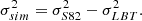
We then followed the procedure outlined in Fig. 1 on the ‘simulated’ IAC Stripe 82 images based on the degraded LBT images and locate the edge of the galaxy. For this particular galaxy, we followed the same masking procedure as that outlined in Trujillo et al. (2021) to ensure the same regions are compared when interpreting the data. The result is shown in Fig. B.1 where we show the radial profiles from LBT (taken from Trujillo et al. (2021)) and the median profile with simulated IAC Stripe 82 depth after 100 separate realisations of random noise. The shaded regions correspond to ± three standard deviations from the median profile plotted up to where the deviation is less than 0.2 mag. From the g − r and Σ⋆ profile, we see that the location of the edge (R = 194″ marked with the vertical dotted line) does not change between the profiles. The main difference is that the profiles are more noisier in the outskirts with IAC Stripe 82 depth but this does not prevent the identification of the edge (although it is certainly harder) using our criteria. For NGC1042, the edge appears at a mass density of 1 M⊙/pc2.
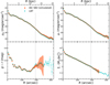 |
Fig. B.1. Radial profiles of NGC1042 from LBT (Trujillo et al. 2021) and simulated IAC Stripe 82 depth (this work, see text for details). The simulated profile is the median of 100 realisations and the shaded regions correspond to ± three standard deviations up to where the deviation from the median is less than 0.2 mag. The vertical grey line is located at the edge of the galaxy (R = 194″). |
B.2. Detecting edges with IAC Stripe 82 depth
In the second part of this appendix, we compare the surface brightness at which the edges of our parent sample appear with the limiting surface brightness of the IAC Stripe 82 images used. We do this by computing the representative depth of each image as it depends on the size of galaxies (i.e. the area near Redge for each galaxy). This can be understood in the following way. In general, the limiting surface brightness of an image can be computed as the xσ fluctuation (where x corresponds to the number of deviations) with respect to the background of the image that is measured over an area A. The form (xσ;A arcsec2) is called a metric. As a rule of thumb, A is optimally chosen according to the apparent size of objects under consideration (using a circle, box etc.). For example in the SDSS g-band, we may write that the limiting surface brightness depth is μlim, g∼ 26.5 mag/arcsec2 (3σ;R = 12”), where A was chosen to be the area of a circle with radius R = 12 (Kniazev et al. 2004). This is a reasonable choice for A because Kniazev et al. (2004) was interested in the search for new dwarf and low surface brightness galaxies in SDSS. To convert the limiting surface brightness (at a given wavelength λ) from metric (x1σ; A1) to (x2σ; A2) is:
![$$ \begin{aligned} \upmu _{lim,\lambda }(x_2\sigma ; A_2) = \upmu _{lim,\lambda }(x_1\sigma ; A_1) - 2.5\log \left[ \frac{x_2}{x_1} \right] + 2.5\log \left[ \frac{A_2}{A_1} \right]^{1/2}, \end{aligned} $$](/articles/aa/full_html/2022/11/aa43612-22/aa43612-22-eq14.gif)
where xk is the number of variations σ and Ak is the area used for k = 1, 2. Given that we know the depth of our images for an area of 10 × 10 arcsec2 (Sect. 3), we can use Eq. B.2 to compute the limit over different areas. We do this for the size of each galaxy in our parent sample in the following way to confirm that the depth of the image is enough to detect their edges.
We plot the observed surface brightness in the g-band at which the edges of the galaxies appear (μg(Redge)) as a function of stellar mass in Fig. B.2. To determine the representative limit of the data given the size of the galaxy, we compute the 3σ limit over the area of pixels in an elliptical annuli (used when deriving the surface brightness profile, see Sect. 4) at Redge for each galaxy. The line of best fit is plotted in black and the grey shaded region bounds the ±1σ dispersion of the fit.
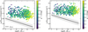 |
Fig. B.2. Observed surface brightness in the g (left) and r-band (right) at Redge (μg(Redge) and μr(Redge) respectively) as a function of stellar mass. The edges appear well-within the 3σ limit of our data computed near Redge (black line, see text for details). |
The figure shows that all the edges appear at surface brightnesses above the limit near Redge, even for the redder galaxies. Therefore, we may conclude that the edges we study here are not a consequence of image depth and the stratification in the size–stellar mass plane is not an observational bias towards bluer edges. In other words, if there were larger galaxies with redder edges in our sample at any fixed stellar mass, we should have been capable of identifying them with our data.
Appendix C: The dependence of radial profile derivation methods on galaxy orientation
Two methods have been mainly used to derive the radial profiles of galaxies in the literature. In the first method, radial profiles are derived along the galaxy’s semi-major axis using a slit of fixed width9. The second method uses elliptical annuli: the axis ratio and position angle to parameterise the ellipse for this procedure may either be fixed (this work) or allowed to vary along the main body of the galaxy. The slit method is generally used to characterise the radial profiles of edge-on oriented galaxies as the method is limited to imaging with high signal-to-noise and edge-on galaxies are naturally observed deeper than face-on ones due to the line-of-sight integration. On the other hand, the ellipse method is limited to galaxies that can be described by an ellipse and this is not the case for edge-on or near edge-on (q ≲ 0.3) galaxies with prominent bulges. Therefore, the ellipse method has been used to derive the profiles of low-inclination galaxies and is possible with lower signal-to-noise imaging.
In this appendix, we study and compare both of these profile derivation methods on an edge-on and low-inclination galaxy to examine its effect on the visibility of the edge and on galaxy orientation. We make use of the LBT data of the low-inclination galaxy NGC1042 as in Appendix B.1 and SDSS DR12 images of the edge-on galaxy UGC09138 shown in Fig. 2.
For the slit method, we used a 1.2 kpc width for both galaxies and we followed the procedure outlined in Sect. 4 for the elliptical annuli method. The result of the comparison is shown in Fig. C.1 for UGC09138 (top panels) and NGC1042 (lower panels). The profiles derived using the slit method is plotted in solid, cyan lines and ellipse method in dashed, black ones. It can be seen that the edge of UGC09138 may only be located using the slit (semi-major) axis method in the μg and Σ⋆ profiles while both methods may be used to locate the edge of NGC1042 in the Σ⋆ profile. However, the edge also becomes clearer in the μg profile of NGC1042 using the slit method. The latter result thus highlights the fact that deeper imaging with higher signal-to-noise than SDSS or IAC Stripe 82 such as LIGHTS and the future LSST will allow the identification and characterisation of edges using the slit method also for near face-on (q ≥ 0.8) galaxies.
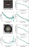 |
Fig. C.1. Comparison between radial profiles derived using a 1.2 kpc slit through the semi-major axis of the galaxy (solid, cyan) and elliptical annuli (dashed, black) for UGC09138 (edge-on, top panels) and NGC1042 (low-inclination, lower panels). The elliptical annuli method is suitable for the low-inclination galaxies studied in this work. See text for details. |
C.1. Dwarf galaxy SDSS J224114.29-003710.2
We have identified Redge using the change in slope in the stellar mass density profile of the dwarf galaxy SDSS J224114.29-003710.2 in Fig. 4. The profiles plotted in that figure were derived using the ellipse method as described above and in Sect. 4. As an example, we also derive the profiles using the slit method, with a 1 kpc width slit through the semi-major axis of the galaxy. The profiles from the two methods are compared in Fig. C.2. We mark Redge as in Fig. C.1 and confirm that both methods have a signature of the edge in the same location. However, while the slit method additionally provides the signature in the g − r profile as a sharp drop towards bluer outskirts, we point out that this feature does not take into account the global colour of the galaxy at Redge because it was strictly computed within the slit region.
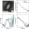 |
Fig. C.2. Comparison between radial profiles derived for the dwarf galaxy SDSS J224114.29-003710.2 using a 1 kpc slit through its semi-major axis (squares, black) and elliptical annuli (dotted, blue). The x-axis and Redge for this galaxy are scaled and marked similarly to Fig. 4. |
Appendix D: Fits to the Σ⋆(Redge)−M⋆ relation
In this appendix, we justify the use of Eqs. 3 and 4 as best fits to the Σ(Redge)−M⋆ relation shown in Fig. 5.
In Fig. D.1, we compare fitting the measurements using two linear fits (as adopted in this work) with a single linear relation and a polynomial of degree 2. We test whether these fitted relations pass through the mean Σ⋆(Redge) in steps of 0.1 dex over our full stellar mass range (107 M⊙ < M⋆ < 1012 M⊙). The grey points show our measurements (Fig. 5), the cyan squares show the mean Σ⋆(Redge) in each stellar mass bin, the pink dot-dashed line shows the single linear fit, the orange dashed line shows the polynomial fit of degree 2 and the purple lines show the linear relationships split at the stellar mass of 1010.5 M⊙ (Eqs. 3 and 4). We mark where the relations split with a vertical dashed black line. The shaded region shows the 1 sigma scatter in the fitted linear relations.
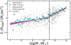 |
Fig. D.1. Fitting functions for the Σ⋆(Redge)−M⋆ relation (grey points). The mean Σ⋆(Redge) is computed in steps of 0.1 dex over the plotted stellar mass range (cyan squares). The best fits (purple lines) are the two linear relations in Eqs. 3 and 4, split at 1010.5 M⊙ (vertical black dashed line). For contrast, we also show a single linear fit (pink dot-dashed line) and polynomial fit of degree two for the full sample (orange dashed line). |
From this figure, it is clear that both the single linear and polynomial fits do not pass through all the mean points (cyan) of the Σ⋆(Redge)–stellar mass plane. The relation also changes slope at a stellar mass of 1010.5 M⊙ (vertical dashed line). These findings do not change if we restrict the single linear fit to galaxies only with stellar masses M⋆ > 109 M⊙, which we confirm by studying the residuals of the fits with respect to the mean data points shown in Fig. D.2. The reduced chi-square values are 1.6 and 1.7 for the purple Σedge(M⋆) relations in Eqs. 3 and 4, 3.1 for the pink linear relation and 2.9 for the polynomial fit, with respect to the mean data points.
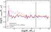 |
Fig. D.2. Comparing the residuals of the fits to the mean Σ⋆(Redge) relation. The single linear fit in pink used here is computed for galaxies with M⋆ > 109 M⊙. The reduced chi-square values are 1.6 and 1.7 for the purple Σedge(M⋆) relations in Eqs. 3 and 4, 3.1 for the pink linear relation and 2.9 for the polynomial fit. |
We also confirm that these results do not change if we exclude the dwarf galaxies in our sample. Therefore, we use the two linear relations as the best fits to our measurements in the Σ⋆(Redge)–stellar mass plane. This choice also leads to comparable sample sizes of galaxies with stellar masses either greater or less than 1010.5 M⊙.
Finally, for the late-type galaxies plotted in Fig. 8, we point out that while the scatter of the relation is large, the Spearman’s correlation coefficient is positive and with a p-value < 1%. This result is an indication that there is a very strong relation in this parameter space even though the scatter is high.
Appendix E: The usability of Redge in large-scale, multi-band surveys
We have visually identified the edges of a large sample of galaxies (645 galaxies). Such a detailed study will no longer be feasible once data will be acquired from wide surveys such as the LSST mentioned above, which is expected to provide 20 TB of data per night10. A natural question is thus how convenient and usable is Redge as a size measure to be included in large-scale galaxy catalogues?
We emphasise that we use the stellar mass density at the location of the edge as a proxy for the underlying theoretical gas density threshold required for star formation in galaxies (see Schaye 2004; Trujillo et al. 2020). For this reason, as an exercise, we used the ⟨Σedge(M⋆)⟩ relations (Eqs. 3 and 4) to ascertain the average location of the edge for each galaxy, ⟨Redge⟩. For each galaxy with stellar mass M⋆ we locate the position of ⟨Σ⋆(Redge)⟩ using the stellar mass density profile of the object: Σ⋆(⟨Redge⟩) = ⟨Σedge(M⋆)⟩. The resulting ⟨Redge⟩–stellar mass relation for the parent sample is shown in Fig. E.1. The ⟨Redge⟩–stellar mass plane also follows a power law of the form 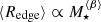 . As expected, the dispersion of this plane is less than that of the observed Redge–stellar mass plane: σ⟨Redge⟩ = 0.093 ± 0.005 dex but the slope is compatible ⟨β⟩ = 0.30 ± 0.006.
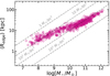 |
Fig. E.1. ⟨Redge⟩–stellar mass relation for the parent sample resulting from the density threshold laws in Eqs. 3 and 4. The structure of the relation is almost exactly the same as the observed Redge–stellar mass relation shown in Fig. 5 which makes it a promising method to determine a proximal measure of Redge automatically for large-scale cataloguing. |
The above result suggests that Eqs. 3 and 4 could potentially be used to obtain ⟨Redge⟩ and provide a proxy for the size of any galaxy, provided its stellar mass is known. These laws can be useful for larger galaxy samples and automated cataloguing in future multi-band surveys such as the LSST. Providing ⟨Redge⟩ is also advantageous for cases where the edge is not apparent and thus serves as a prediction of where the edge should be for a given galaxy. Strong deviations from this prediction could then provide insights about the stellar population properties in the outskirts of the galaxy in comparison with the parent population.
We point out that galaxies with low stellar density and mass (i.e. low surface brightness galaxies, e.g. Sandage & Binggeli (1984)) are not included in our sample and the validity of Eqs. 3 and 4 to such galaxies need to be investigated in future work (but see Chamba et al. 2020).
All Tables
All Figures
|
Fig. 1. Flowchart illustrating the visual identification of edges. An example of a galaxy, SDSS J003143.28+005402.4, and its profiles with the identified edge (vertical dotted line) is shown in the top right side of the flowchart. If the galaxy is symmetric, the relevant parameters in the edge, namely, Redge, the colour and mass density at the edge are saved. However, if the galaxy contains any non-symmetric features such as tidal streams in its outskirts such as the example SDSS J012859.56−003342.96 shown in the lower section of the flowchart, they are masked and the process of finding the edge is attempted once again. No edges are reported for cases when even an improvement in the masking did not present an edge. See Sect. 5.1 for details. |
| In the text | |
|
Fig. 2. Edges of galaxies as viewed in edge-on (left) to face-on (right) orientations. The galaxies were selected to have similar rotational velocities Vrot ∼ 145 km s−1. Left to right: IAC Stripe 82 gri-colour composite image overlaid on a grey scaled gri-band summed image for contrast, surface brightness profiles in the SDSS g, r, GALEX NUV and FUV bands, g − r colour profile and the corresponding Σ⋆ stellar mass density profile. The pink contour in the gri-image and the vertical dotted lines in the other panels indicate the edge of the galaxy. |
| In the text | |
|
Fig. 3. Three examples of elliptical galaxies from the parent sample with stellar mass ∼1011 M⊙. Top: gri-band colour composite images, overlaid on the background gri summed image in grey scale, of the galaxies denoted as A (left), B (middle) and C (right). The SDSS J2000 identifier and Redge are labelled for these galaxies as in Fig. 2. Bottom, left to right: the μg, g − r and Σ⋆ profiles of the objects. The edges for these galaxies are visible as a sudden transition from red to blue in their g − r colour profiles (see Sect. 5.3 for details). The locations of the edges occur at mass densities Σ⋆(Redge) > 1 M⊙ pc−2. |
| In the text | |
|
Fig. 4. Similar to Fig. 3, but for three dwarf galaxies with stellar mass ∼108 M⋆. These examples were specifically chosen to illustrate the diversity in the colour profiles of this galaxy population and the criteria we use to we locate the edge in these different cases. In case A, we use the change in slope in the Σ⋆ profile. In B and C, the edge is identified as a sudden transition to bluer colours in the g − r profile (see Sect. 5.4 for details). The edges of these galaxies occur at mass densities Σ⋆(Redge)≲2 M⊙ pc−2. |
| In the text | |
|
Fig. 5. Redge–stellar mass (left) and Σ⋆(Redge)–stellar mass (right) relations derived in this work. Only those galaxies where an edge was identified are plotted (624 objects). The grey lines in the Redge–stellar mass planes are lines of constant stellar mass surface density within the Redge of the object. Top to bottom: each row shows the same observed relations (top), colour coded according to the morphology of the galaxies, (g − r)edge and a proxy for the age at Redge, for a fixed metallicity [M/H]= − 0.71. We plot the uncertainties in our measurements (see Sect. 4) only in the second row for clarity in the other panels. |
| In the text | |
|
Fig. 6. Similar to Fig. 5, now including the measurements in this work for the sample of galaxies studied in B12 and P17. The grey circles are the measurements for our sample. |
| In the text | |
|
Fig. 7. Representation of the results shown in Fig. 5 as histograms. Top: the distribution of Redge (left) and Σ⋆(Redge). Bottom: the distribution of (g − r)edge in the Redge–stellar mass (left) and Σ⋆(Redge)–stellar mass (right) relations. The subscript ‘fit’ refers to the best fit line of each plane. |
| In the text | |
|
Fig. 8. Stratification of late-type galaxies in the Redge–stellar mass (left) and Σ⋆(Redge)–stellar mass (right) relation. The galaxies are grouped morphologically following Trujillo et al. (2020). The lines are the best-fit relations for each group in both panels. See text for details. |
| In the text | |
|
Fig. 9. Ratios Redge/Re (left) and R1/Re (right) as a function of the respective sizes for the labelled morphologies. The diagrams reinforce how extended galaxies are compared to what the effective radius represents Re. |
| In the text | |
|
Fig. 10. Comparison between Redge and R1. The top and middle panels show Redge vs. R1 for the galaxies in our sample, colour coded in stellar mass and morphology, respectively. The solid black line in the upper panels is the one-to-one relation. The lower panel shows the same distribution as a histogram. |
| In the text | |
|
Fig. 11. R1 of galaxies where we were unable to locate the presence of edges (black) over plotted on the Redge–stellar mass plane (pink). |
| In the text | |
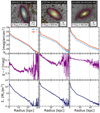 |
Fig. A.1. Radial profiles of three difficult cases. The panels are labelled as in Fig. 2. |
| In the text | |
|
Fig. B.1. Radial profiles of NGC1042 from LBT (Trujillo et al. 2021) and simulated IAC Stripe 82 depth (this work, see text for details). The simulated profile is the median of 100 realisations and the shaded regions correspond to ± three standard deviations up to where the deviation from the median is less than 0.2 mag. The vertical grey line is located at the edge of the galaxy (R = 194″). |
| In the text | |
|
Fig. B.2. Observed surface brightness in the g (left) and r-band (right) at Redge (μg(Redge) and μr(Redge) respectively) as a function of stellar mass. The edges appear well-within the 3σ limit of our data computed near Redge (black line, see text for details). |
| In the text | |
|
Fig. C.1. Comparison between radial profiles derived using a 1.2 kpc slit through the semi-major axis of the galaxy (solid, cyan) and elliptical annuli (dashed, black) for UGC09138 (edge-on, top panels) and NGC1042 (low-inclination, lower panels). The elliptical annuli method is suitable for the low-inclination galaxies studied in this work. See text for details. |
| In the text | |
|
Fig. C.2. Comparison between radial profiles derived for the dwarf galaxy SDSS J224114.29-003710.2 using a 1 kpc slit through its semi-major axis (squares, black) and elliptical annuli (dotted, blue). The x-axis and Redge for this galaxy are scaled and marked similarly to Fig. 4. |
| In the text | |
|
Fig. D.1. Fitting functions for the Σ⋆(Redge)−M⋆ relation (grey points). The mean Σ⋆(Redge) is computed in steps of 0.1 dex over the plotted stellar mass range (cyan squares). The best fits (purple lines) are the two linear relations in Eqs. 3 and 4, split at 1010.5 M⊙ (vertical black dashed line). For contrast, we also show a single linear fit (pink dot-dashed line) and polynomial fit of degree two for the full sample (orange dashed line). |
| In the text | |
|
Fig. D.2. Comparing the residuals of the fits to the mean Σ⋆(Redge) relation. The single linear fit in pink used here is computed for galaxies with M⋆ > 109 M⊙. The reduced chi-square values are 1.6 and 1.7 for the purple Σedge(M⋆) relations in Eqs. 3 and 4, 3.1 for the pink linear relation and 2.9 for the polynomial fit. |
| In the text | |
|
Fig. E.1. ⟨Redge⟩–stellar mass relation for the parent sample resulting from the density threshold laws in Eqs. 3 and 4. The structure of the relation is almost exactly the same as the observed Redge–stellar mass relation shown in Fig. 5 which makes it a promising method to determine a proximal measure of Redge automatically for large-scale cataloguing. |
| In the text | |
Current usage metrics show cumulative count of Article Views (full-text article views including HTML views, PDF and ePub downloads, according to the available data) and Abstracts Views on Vision4Press platform.
Data correspond to usage on the plateform after 2015. The current usage metrics is available 48-96 hours after online publication and is updated daily on week days.
Initial download of the metrics may take a while.