| Issue |
A&A
Volume 675, July 2023
BeyondPlanck: end-to-end Bayesian analysis of Planck LFI
|
|
|---|---|---|
| Article Number | A16 | |
| Number of page(s) | 15 | |
| Section | Cosmology (including clusters of galaxies) | |
| DOI | https://doi.org/10.1051/0004-6361/202243410 | |
| Published online | 28 June 2023 | |
From BEYONDPLANCK to COSMOGLOBE: Preliminary WMAP Q-band analysis
1
Institute of Theoretical Astrophysics, University of Oslo, Blindern, Oslo, Norway
e-mail: duncanwa@astro.uio.no
2
Dipartimento di Fisica, Università degli Studi di Milano, Via Celoria, 16, Milano, Italy
3
INAF/IASF Milano, Via E. Bassini 15, Milano, Italy
4
INFN, Sezione di Milano, Via Celoria 16, Milano, Italy
5
INAF – Osservatorio Astronomico di Trieste, Via G.B. Tiepolo 11, Trieste, Italy
6
Planetek Hellas, Leoforos Kifisias 44, Marousi, 151 25
Greece
7
Department of Astrophysical Sciences, Princeton University, Princeton, NJ, 08544
USA
8
Jet Propulsion Laboratory, California Institute of Technology, 4800 Oak Grove Drive, Pasadena, CA, USA
9
Department of Physics, Gustaf Hällströmin katu 2, University of Helsinki, Helsinki, Finland
10
Helsinki Institute of Physics, Gustaf Hällströmin katu 2, University of Helsinki, Helsinki, Finland
11
Computational Cosmology Center, Lawrence Berkeley National Laboratory, Berkeley, CA, USA
12
Haverford College Astronomy Department, 370 Lancaster Avenue, Haverford, Pennsylvania, USA
13
Max-Planck-Institut für Astrophysik, Karl-Schwarzschild-Str. 1, 85741 Garching, Germany
14
Dipartimento di Fisica, Università degli Studi di Trieste, Via A. Valerio 2, Trieste, Italy
Received:
23
February
2022
Accepted:
6
July
2022
We present the first application of the COSMOGLOBE analysis framework by analyzing nine-year WMAP time-ordered observations that uses similar machinery to that of BEYONDPLANCK for the Planck Low Frequency Instrument (LFI). We analyzed only the Q-band (41 GHz) data and report on the low-level analysis process based on uncalibrated time-ordered data to calibrated maps. Most of the existing BEYONDPLANCK pipeline may be reused for WMAP analysis with minimal changes to the existing codebase. The main modification is the implementation of the same preconditioned biconjugate gradient mapmaker used by the WMAP team. Producing a single WMAP Q1-band sample requires 22 CPU-hrs, which is slightly more than the cost of a Planck 44 GHz sample of 17 CPU-hrs; this demonstrates that a full end-to-end Bayesian processing of the WMAP data is computationally feasible. In general, our recovered maps are very similar to the maps released by the WMAP team, although with two notable differences. In terms of temperature, we find a ∼2 μK quadrupole difference that most likely is caused by different gain modeling, while in polarization we find a distinct 2.5 μK signal that has been previously referred to as poorly measured modes by the WMAP team. In the COSMOGLOBE processing, this pattern arises from temperature-to-polarization leakage from the coupling between the CMB Solar dipole, transmission imbalance, and sidelobes. No traces of this pattern are found in either the frequency map or TOD residual map, suggesting that the current processing has succeeded in modeling these poorly measured modes within the assumed parametric model by using Planck information to break the sky-synchronous degeneracies inherent in the WMAP scanning strategy.
Key words: ISM: general / cosmology: observations / cosmic background radiation / diffuse radiation / Galaxy: general
© The Authors 2023
 Open Access article, published by EDP Sciences, under the terms of the Creative Commons Attribution License (https://creativecommons.org/licenses/by/4.0), which permits unrestricted use, distribution, and reproduction in any medium, provided the original work is properly cited.
This article is published in open access under the Subscribe to Open model. Subscribe to A&A to support open access publication.
1. Introduction
Since the discovery of the cosmic microwave background (CMB; Penzias & Wilson 1965), there have been three generations of groundbreaking satellite missions to characterize the spatial and frequency properties of the microwave sky; the Cosmic Background Explorer (COBE; Smoot et al. 1992; Mather et al. 1994), the Wilkinson Microwave Anisotropy Probe (WMAP; Bennett et al. 2013), and Planck (Planck Collaboration I 2020). Current and future experiments designed to detect primordial gravitational waves due to inflation (e.g., Kamionkowski & Kovetz 2016, and references therein) are built on the foundations of these satellite missions.
The field of CMB cosmology has generally followed a model in which the data from previous experiments are first complemented, then gradually improved upon and superseded by those that follow. One example is COBE/DMR, in operation between 1989 and 1994, which discovered primordial CMB anisotropies at 31.5, 53, and 90 GHz with a resolution of 7° (Smoot et al. 1992). Together with the COBE/FIRAS measurement of the CMB blackbody spectrum (Mather et al. 1994), these observations led to the Nobel Prize in Physics in 2006. While COBE/DMR observations were groundbreaking in their time, they have rarely been directly used for cosmological analysis after the WMAP team released their sky maps in 2003 (Bennett et al. 2003b), which improved on DMR in terms of angular resolution and sensitivity by orders of magnitude. When the Planck mission released its sky maps in 2013 (Planck Collaboration I 2014), they included higher sensitivity, finer angular resolution, and wider frequency coverage, providing tighter constraints on both cosmological parameters and Galactic physics.
Established data sets remain crucial in the analysis of current and future data sets, both for calibration and testing, but also for breaking degeneracies beyond their original primary science goals. One prominent example is the WMAP K-band sky map at 23 GHz (Bennett et al. 2013), which (after Planck) represents the highest signal-to-noise ratio tracer of polarized synchrotron emission and is therefore used extensively for foreground modeling. More generally, the five WMAP frequencies provide essential constraining power for low-frequency CMB foregrounds and it is only through the combination of Planck and WMAP observations (and other data sets) that it is possible to individually constrain the properties of synchrotron, free-free, and anomalous microwave emission (AME) over the full sky (e.g., Planck Collaboration X 2016; Andersen et al. 2023).
A second important example is COBE/FIRAS (Mather et al. 1994), which showed that the CMB is well described by the Planck blackbody radiation law at a temperature of T = 2.72548 ± 0.00057 K (Fixsen 2009); despite being now more than 20 years old, this experiment has not yet been improved upon, and all later CMB experiments rely directly on this value as a strong prior for calibration purposes (e.g., Bennett et al. 2013; Planck Collaboration V 2020; Gjerløw et al. 2023). A third example is the COBE/DIRBE experiment (Hauser et al. 1998), which still represents a state-of-the-art approach in terms of submillimeter zodiacal light observations (Kelsall et al. 1998; Planck Collaboration XIV 2014), due to its unique combination of frequency and sky coverage. A final example is the 408 MHz map of Haslam et al. (1982), which is widely used as a template for Galactic synchrotron emission. There have been attempts to improve its quality, for instance, Remazeilles et al. (2015), and despite its noise properties not being fully characterized, this map is still widely used in foreground studies.
Each of these data sets faces major challenges with regard to how systematic error correction and uncertainty propagation are handled. In most cases, data are provided to the public in the form of processed high-level products (most typically pixelized sky maps, angular power spectra, or cosmological parameters); at these levels, it is difficult to assess the impact of instrumental effects such as calibration, beam and sidelobe errors, and correlated noise. This in turn limits the usefulness of older data sets, as the systematic error requirements of next-generation experiments are more stringent than those of previous generations. A major concern is whether direct joint analyses between old and new data sets may contaminate the latter. For almost any new experiment, there is a tension between the desire of including complementary data sets to break degeneracies to which one’s own experiment is not sensitive, versus the concern of introducing uncontrolled systematics into the analysis.
COSMOGLOBE1 aims to solve this problem by developing a common analysis platform that is applicable to a wide range of radio, microwave, and submillimeter experiments; legacy, current, and future. A joint analysis of complementary experiments is essential to break instrumental and astrophysical parameter degeneracies. Therefore, as more data sets are added to this analysis, better cosmological and astrophysical results will emerge. Enabling and organizing this work is the main goal of the community-wide and Open Science COSMOGLOBE program.
BEYONDPLANCK represents the first stage of the process, in which the Planck Low Frequency Instrument (LFI; Planck Collaboration VI 2014; Planck Collaboration II 2016, 2020) data are processed within a global Bayesian framework. This data set was chosen for three reasons; (1) the LFI data volume is relatively low, allowing for fast debugging; (2) the LFI instrumental systematics are well understood; and (3) the current team members have years of experience working with this data set.
In this paper, we generalize the same framework to support WMAP time domain analysis. We note that a full WMAP reanalysis lies outside the scope of the present paper, as this would require both additional modeling and analysis effort. Rather, the main goals of the current work are to answer the following practical questions: First, how much software development effort is required to generalize the Commander software to support an entirely new data set. Second, whether a proper end-to-end Bayesian analysis of the full WMAP data set is technically feasible with currently available computing power and, if so, how much computational power this would entail. Third, we consider what additional instrument-specific features are required to perform a full WMAP analysis. These questions are important not only for a future WMAP reanalysis itself, but also for other experiments that may adopt the Commander framework for their own analysis. In implementing a WMAP pipeline using Commander, we demonstrate that this Bayesian framework can be generalized to data sets beyond the one it was explicitly designed to analyze (Planck LFI).
2. Bayesian WMAP analysis with Commander
2.1. BeyondPlanck data model and posterior distribution
The BEYONDPLANCK framework (BeyondPlanck Collaboration 2023) takes a novel approach to CMB data analysis by adopting a strictly parametric Bayesian end-to-end formulation. As for any parametric Bayesian calculation, the first step in implementing the algorithm is writing down an explicit parametric data model; everything else will then, ideally, follow naturally from that model. The data model adopted for Planck LFI takes the form:
![$$ \begin{aligned} d_{t,j}=g_{t,j} \mathsf P _{tp,j}\left[ \mathsf B _{j}^\mathrm{mb} s_{j}^\mathrm{sky} + \mathsf B _{j}^\mathrm{fsl} s_{j}^{\mathrm{sky} } +\mathsf B _{j}^\mathrm 4\pi s_{t,j}^\mathrm{orb} \right] + s_{t,j}^\mathrm{1\,Hz }+n_{t,j}^\mathrm{corr} +n_{t,j}^w, \end{aligned} $$](/articles/aa/full_html/2023/07/aa43410-22/aa43410-22-eq1.gif)
where t indexes the observation time, j indexes the detector, p indexes the pixel, gt, j is a time-dependent gain, Ptp, j is a pointing matrix, B includes components of the beam (main beam Bmb, far sidelobes Bfsl, and full B4π, respectively),  is the (time-independent) sky signal,
  is the orbital CMB dipole,
  is the (orientation-dependent) far sidelobe contribution,
  is a contribution from electronic 1 Hz spikes,
  is the correlated noise, and
  is the white noise. We note that the 1 Hz spikes are unique to Planck LFI, and are not used in the WMAP analysis. The parametric sky model ssky(ν, a, β) includes contributions from CMB, synchrotron, free-free, spinning dust, thermal dust, and point source emission. A full description of the sky model can be found in BeyondPlanck Collaboration (2023).
The data model may be written in a compact vector form:

where we have now also introduced the diagonal gain matrix Gj = diag(gt, j) and the mixing matrix M to describe bandpass integration effects,
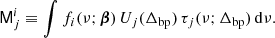
Here, τj is the bandpass for each detector with a free parameter Δbp, Uj converts from a brightness-temperature to frequency-sky map unit integrated over the bandpass (Planck Collaboration IX 2014), fi(ν; β) is the spectral energy distribution (SED) of component, i, given the generalized SED parameters β, and n = ncorr + nwn. For LFI, n is often assumed to be Gaussian distributed with a covariance matrix, N, given by a 1/f power spectral density (PSD),
![$$ \begin{aligned} \mathcal{P} (f) = \sigma ^2[1+(f/f_{\mathrm{knee} })^\alpha ], \end{aligned} $$](/articles/aa/full_html/2023/07/aa43410-22/aa43410-22-eq10.gif)
where σ is the white noise standard deviation, fknee is the correlated noise knee frequency, and α is the correlated noise spectral index. In general, we denote the set of all noise PSD parameters as ξn. For a full discussion of this model, we refer the interested reader to BeyondPlanck Collaboration (2023) and references therein.
Let us now denote the set of all free parameters in Eqs. (1)–(3) by ω, such that ω = {g, ncorr, β, a, …}. The Bayesian approach is to map out the posterior distribution,

using standard Markov chain Monte Carlo (MCMC) sampling methods, where ℒ(ω) is the likelihood function and P(ω) is the prior probability of the vector ω. We define the likelihood by assuming that the noise component in Eq. (2) is Gaussian distributed, such that:

The priors are in general less well-defined, and in practice we use both algorithmic and informative priors to ensure a robust fit; we refer, for example, BeyondPlanck Collaboration (2023) and Andersen et al. (2023). For the special case of the CMB, it is common to assume that its fluctuations are isotropic and Gaussian distributed, with a variance given by the angular power spectrum, Cℓ; estimating this power spectrum is typically a main goal for most CMB experiments.
The posterior distribution defined by Eq. (5) is infeasible to map out directly, due to the sheer number of free parameters and degeneracies within the model. However, the Gibbs sampling algorithm (Gelman & Rubin 1992) allows for efficient exploration of the full joint distribution by iterating through all conditional distributions, each of which are simpler to explore than the full joint distribution. To be specific, the BEYONDPLANCK Gibbs chain takes the form (BeyondPlanck Collaboration 2023):


where ← denotes drawing a sample from the conditional distribution on the right. In the Commander framework, CMB analysis essentially amounts to repeating each of these steps until convergence, which typically requires thousands of iterations.
In this work, we hold the amplitude and SED parameters a and β fixed, as our goal is to determine the feasiblility of extending the time-ordered data (TOD) analysis to the WMAP data set. In a full analysis, we would perform a full Gibbs chain on all of these parameters jointly, but in this paper we first fit the sky model using almost the same data combination as BeyondPlanck Collaboration (2023), namely, Planck LFI 30–70 GHz, Planck HFI 353 (in polarization), and 857 GHz (in temperature), WMAP9 Ka–V, and Haslam 408 MHz. However, unlike the main analysis, we additionally include the WMAP9 K-band data to increase the signal-to-noise ratio for low-frequency foreground components. We then use this fixed sky model throughout to calibrate the Q1 data. This yields a simplified Gibbs chain:


which holds all sky and bandpass parameters fixed throughout.
2.2. Generalization to WMAP
The WMAP mission (Bennett et al. 2013) observed the sky at K, Ka, Q, V, and W-bands (23, 33, 41, 61, and 94 GHz, respectively) using differential radiometers, from August 10, 2001 to August 10, 2010. The satellite observed from the second Sun-Earth Lagrange point with a Lissajous orbit, rotating around its primary axis with a period of 129 s, and precessing around its spin axis with a period of one hour, allowing for total coverage of the sky every six months. This observing strategy allowed for excellent control of systematic effects that appear in the time streams (Bennett et al. 2003a).
The WMAP instrument is inherently differential, with each detector recording the signal difference received in two horns, labeled A and B. Each radiometer is sensitive to two orthogonal polarization directions, γ and γ + π/2, and each of these are coupled pairwise with the two horns, such that each radiometer ultimately results in four polarized time streams, which are treated jointly in a single differencing assembly (DA). WMAP has ten total DAs, one for both K and Ka, two each for Q and V, and four for W. In this paper, we consider the DA corresponding to Q1, whose individual time streams are indexed by Q1ij, where i ∈ {1, 2} labels the detector’s polarization orientation, and j ∈ {3, 4} labels the sA − sB and sB − sA time streams.
The primary goal of the current paper is to understand what is required in terms of coding efforts and computational resources in order to apply the Commander framework as summarized above to the WMAP data. The first step in that process is to write down an explicit parametric data model. When one reviews the descriptions of the WMAP instrument and time-ordered data provided by Bennett et al. (2003b), Barnes et al. (2003), Jarosik et al. (2003, 2007), Hinshaw et al. (2003), Page et al. (2007), and Greason et al. (2012), it becomes clear that the LFI data model defined in Eq. (1) also applies to WMAP with only three modifications: two major and one minor. We go on to address each of these in turn below.
First, while Planck measures the power received from a single point on the sky, WMAP records the difference between two points in digital units (du),
![$$ \begin{aligned} \begin{aligned} s= g\big [\,&\alpha _\mathrm{A} (T_\mathrm{A} + Q_\mathrm{A} \cos 2\gamma _\mathrm{A} +U_\mathrm{A} \sin 2\gamma _\mathrm{A} ), \\ \,-&\alpha _\mathrm{B} (T_\mathrm{B} + Q_\mathrm{B} \cos 2\gamma _\mathrm{B} +U_\mathrm{B} \sin 2\gamma _\mathrm{B} )\big ]. \end{aligned} \end{aligned} $$](/articles/aa/full_html/2023/07/aa43410-22/aa43410-22-eq23.gif)
In this equation, {T, Q, U} are the Stokes parameters seen by each horn, and αA/B is a horn transmission coefficient that quantifies the transmission of the optics and waveguide components, which may be slightly different between the two sides. Following Hinshaw et al. (2003), the transmission coefficients are written in terms of horn imbalance parameters xim that explicitly parameterize the difference between the A and B horn transmissions,
The overall normalization is absorbed into the gain, so that the data model becomes:
![$$ \begin{aligned} \begin{aligned} s= g\big [\,&(1+x_{\mathrm{im} })(T_\mathrm{A} + Q_\mathrm{A} \cos 2\gamma _\mathrm{A} +U_\mathrm{A} \sin 2\gamma _\mathrm{A} ), \\ \,-&(1-x_\mathrm{im} )(T_\mathrm{B} + Q_\mathrm{B} \cos 2\gamma _\mathrm{B} +U_\mathrm{B} \sin 2\gamma _\mathrm{B} )\big ]. \end{aligned} \end{aligned} $$](/articles/aa/full_html/2023/07/aa43410-22/aa43410-22-eq25.gif)
Equation (19) may now be implemented in the LFI data model in Eq. (1) by redefining the pointing matrix, such that a single row reads
![$$ \begin{aligned} \mathsf P _{tp}= \left[ \begin{array}{c} 0\\ \vdots \\ 0\\ (1+x_{\mathrm{im} })\\ (1+x_{\mathrm{im} })\cos 2\gamma _\mathrm{A} \\ (1+x_{\mathrm{im} })\sin 2\gamma _\mathrm{A} \\ 0\\ \vdots \\ 0\\ -(1-x_{\mathrm{im} })\\ -(1-x_{\mathrm{im} })\cos 2\gamma _\mathrm{B} \\ -(1-x_{\mathrm{im} })\sin 2\gamma _\mathrm{B} \\ 0\\ \vdots \\ 0\\ \end{array} \right]^T .\end{aligned} $$](/articles/aa/full_html/2023/07/aa43410-22/aa43410-22-eq26.gif)
Therefore, the fact that WMAP records differential pointing, whereas Planck records the signal from a single point in the sky. This implies that the WMAP pointing matrix has twice as many entries as for LFI and that there is also an additional uncertain parameter per radiometer that needs to be sampled for WMAP, the transmission imbalance parameter. In terms of implementation, this also means that the most important generalization required for Bayesian analysis of WMAP is the implementation of a mapmaker for differential data. This task has already been addressed by the WMAP team, who showed that a stabilized biconjugate gradient method works well for this problem (Jarosik et al. 2011). The main recoding effort done in this paper is thus to reimplement this method in Commander, as discussed in Sect. 3.3.
The second main difference between WMAP and LFI as defined by Eq. (1) lies in the noise model. While the LFI noise is close to white at high temporal frequencies and can be described well with a 1/f model (or, at least, as a sum of a 1/f model and a subdominant Gaussian peak; see Ihle et al. 2023), the WMAP noise is in general colored close to the Nyquist frequency, typically exhibiting a very slight power increase at the highest frequencies. This does have some important sampling technical implications for the noise PSD Gibbs step, as defined in Eq. (9) and discussed by Ihle et al. (2023). The current LFI implementation assumes that the noise is white at the sampling frequency and explicitly uses this to break a degeneracy between the correlated and white noise components. At the same time, the amplitude of this WMAP colored high-frequency noise is very modest, and as shown in Sect. 4, a standard 1/f model does fit reasonably well. Furthermore, a suboptimal noise model will result in slightly suboptimal uncertainties, but not biases. Therefore, this is a minor issue for the purposes of the current paper, which is aimed at assessing the overall applicability of the Bayesian approach for WMAP; low-level noise modeling issues do not affect this approach. We also note that we need to generalize the current noise model to allow for analysis of Planck HFI and other bolometer experiments. An expansion of the Commander noise model has therefore been left for a future work. The third and final difference between LFI and WMAP are electronic 1 Hz spikes, which are not relevant for WMAP. This term is therefore omitted in the following WMAP analysis.
All other parameters and sampling steps in Eqs. (1)–(13) are identical between LFI and WMAP. Since the two experiments cover roughly the same frequency range and angular scales, no new astrophysical components need to be added to the sky model (with the possible exception of HCN and other line emission at W-band, as discussed by Planck Collaboration X 2016), and the required low-level algorithms for sidelobe convolution and orbital dipole generation are identical between the two experiments. Thus, WMAP is an excellent example of the benefits of joint analysis within a single computational framework; nearly all of the existing computer code is directly reusable.
3. Algorithmic details
In this section, we consider in greater detail the four specific algorithmic changes that are necessary for WMAP processing within the Commander framework, namely: (1) handling of compressed TODs; (2) transmission imbalance sampling; (3) mapmaking with differential data; and (4) noise modeling, which are all summarized in Sects. 3.1–3.4. In addition, we review the Commander approach to sidelobe corrections in Sect. 3.5. We summarize the algorithmic differences between WMAP and COSMOGLOBE in Sect. 3.6.
3.1. Data compression
The full nine-year WMAP data set2 spans 626 GB, which has represented a major challenge with respect to optimal mapmaking using all available data in 2013, simply due to computer hardware limitations. In practice, this was overcome by processing each year of observations separately, and then creating a noise-weighted average of the maps. During mapmaking, the TOD were processed in one hour or daily chunks (Bennett et al. 2013).
Today, we circumvent these data volume issues two different ways within Commander. First, having access to large-memory compute nodes with 1.5 TB of RAM greatly alleviates hardware based concerns. This is further improved by storing the TOD in a compressed format in RAM, not only on disk. Specifically, as described by Galloway et al. (2023a), the current pipeline uses Huffman compression to store the TOD, which reduces the number of bits per stored number according to the frequency of that same number. This technique is particularly powerful for the WMAP data, as illustrated in Fig. 1. The most striking feature of this data stream is its discreteness, imposed by the analog-to-digital converter; while the data are delivered in terms of 32-bit integers, typically only 50 of those are encountered in any given data segment. Therefore, relabeling the relevant integers with shorter bit strings yields a significant reduction in data volume. We find that the entire WMAP TOD only requires 186 GB of disk storage after Huffman compression, at which point they may be stored in RAM even on inexpensive modern compute nodes3.
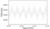 |
Fig. 1. Sample of WMAP TOD. This Q113 datastream was recorded on July 7, 2003. At this resolution, the discreteness of the digital units is apparent, a property which makes these data highly compressible. |
While WMAP used either one or 24 h chunk sizes for their TOD processing (Bennett et al. 2013), we adopted one week periods for our processing. This choice is informed by the extremely low levels of correlated noise in the WMAP data, with fknee ≲ 1 mHz for half of the radiometers (Jarosik et al. 2003), corresponding to 20 min or more in the time domain. With one week time chunks, it is easier to disentangle white and correlated noise and the processing is less sensitive to Fourier-filtering edge effects and aliasing.
3.2. Gain and imbalance sampling
For the purposes of gain sampling, as symbolically defined by Eq. (7), we can simplify the global parametric model in Eq. (1) to:
where  is the full beam-convolved sky signal in time domain for radiometer j. For WMAP, this model may be generalized to differential data with imbalance parameters xim as:
![$$ \begin{aligned} d_{t,j} = g_{t,j}[(1+x_{\mathrm{im} ,j})s_{t,j}^{\mathrm{tot} ,A} - (1-x_{\mathrm{im} ,j})s_{t,j}^{\mathrm{tot} ,B}] +n_{t,j}^\mathrm{corr} + n_{t,j}^\mathrm{wn} . \end{aligned} $$](/articles/aa/full_html/2023/07/aa43410-22/aa43410-22-eq29.gif)
To sample gt, j, we adopt the standard BEYONDPLANCK procedure without modification and define gt, j = g0 + Δgj + δgt, j. Here, g0 denotes the time-independent absolute calibration for the entire DA, Δgj represents the time-independent offset from g0 for the radiometer j, and δgt, j represents the time-dependent fluctuations around the mean for radiometer, j. Each of these three terms is sampled conditionally using its own tuned algorithm. Specifically, g0 is sampled using the orbital CMB dipole only as a calibration source, Δgj is sampled using the full astrophysical sky model, including the Solar dipole, and δgt, j is sampled using an optimal Wiener filter algorithm that weights time-variable fluctuations according to their relative signal-to-noise ratio. For full details, we refer to Gjerløw et al. (2023).
From Eq. (22), we see that xim, j plays a role that is similar to g0 + Δgj. However, unlike those parameters, it applies to pairs of time streams, and for the Q1 DA we estimate the transmission imbalance for Q11 using time streams Q113 and Q114, and the transmission imbalance for Q12 using time streams Q123 and Q124.
To sample xim, we follow Hinshaw et al. (2003) and define the following differential (d) and common-mode (c) signals:
such that
![$$ \begin{aligned} d_{t,j}=g_{t,j}[s_{t,j}^\mathrm{d} +x_{\mathrm{im} ,j}{s_{t,j}^\mathrm{c} }] +n_{t,j}^\mathrm{corr} +n_{t,j}^\mathrm{wn} . \end{aligned} $$](/articles/aa/full_html/2023/07/aa43410-22/aa43410-22-eq32.gif)
If we now form the residual  and define
  , the equation for the residual becomes:

Since we assume the noise is Gaussian distributed with covariance, N, and both T and sc are conditionally fixed, the appropriate conditional distribution for xim, j is also a Gaussian. We can therefore follow the standard procedure outlined in Appendix A.2 of BeyondPlanck Collaboration (2023), and sample xim through the following equation:

where η ∼ N(0, I) is a vector of standard Gaussian random variates. This may be written explicitly as:
![$$ \begin{aligned} x_{\mathrm{im} ,j}= \frac{\sum _{i,t,t^\prime }[g_{i,t}s_{i,c,t}^\mathrm{c} ] \mathsf N ^{-1}_{tt^\prime }r_{i,t^\prime }}{\sum _{i,t,t^\prime }[g_{i,t}s_{i,t,c}^\mathrm{c} ] \mathsf N ^{-1}_{tt^\prime }[g_{i,t^\prime }s_{i,t^\prime ,c}^\mathrm{c} ]} + \frac{\sum _{i,t,t^\prime }[g_{i,t}s_{i,c,t}^\mathrm{c} ] \mathsf N ^{-1/2}_{tt^\prime }\eta _{t^\prime }}{\sum _{i,t,t^\prime }[g_{i,t}s_{i,t,c}^\mathrm{c} ] \mathsf N ^{-1}_{tt^\prime }[g_{i,t^\prime }s_{i,t^\prime ,c}^\mathrm{c} ]},\nonumber \end{aligned} $$](/articles/aa/full_html/2023/07/aa43410-22/aa43410-22-eq37.gif)
where i corresponds to the data streams for radiometer pair j.
3.3. Mapmaking
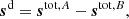
While most instrumental parameters are sampled in the time domain in the Bayesian framework, astrophysical parameters are still sampled in terms of pixelized sky maps. We therefore need to compute coadded maps for each DA. The starting point of this process is the calibrated residual,
where we condition on all instrumental parameters, including g, ncorr, ξn, and xim. In this expression, we have also defined:
which is the difference between the sky signal seen by radiometer j and the same averaged over all radiometers in the given DA. This term accounts for spurious bandpass leakage effects without solving for a spurious map per pixel, as discussed by Svalheim et al. (2023).
Inserting Eq. (28) into the data model in Eq. (1), we find
![$$ \begin{aligned} =&\,(1+x_{\mathrm{im} ,j})[T_{p_\mathrm{A} }+P_{p_\mathrm{A} }(\gamma _{\mathrm{A} ,t})], \nonumber \\&-(1-x_{\mathrm{im} ,j})[T_{p_\mathrm{B} }+P_{p_\mathrm{B} }(\gamma _{\mathrm{B} ,t})] +n_{t,j}, \end{aligned} $$](/articles/aa/full_html/2023/07/aa43410-22/aa43410-22-eq41.gif)
where we denote the total polarized signal as PpA/B(γA/B, t) = QpA/B, tcos2γA/B, t + UpA/B, tsin2γA/B, t. Following Jarosik et al. (2011), we combine these calibrated data into an “intensity” time stream, dt, and a “polarization” time stream, pt,
![$$ \begin{aligned}&=T_{p_\mathrm{A} }-T_{p_\mathrm{B} } +\bar{x}_\mathrm{im} [T_{p_\mathrm{A} }+T_{p_\mathrm{B} }], \nonumber \\&\,\,\,\,\,\,\,\,+\delta x_\mathrm{im} [P_{p_\mathrm{A} }(\gamma _\mathrm{A} )+P_{p_\mathrm{B} }(\gamma _\mathrm{B} )], \end{aligned} $$](/articles/aa/full_html/2023/07/aa43410-22/aa43410-22-eq43.gif)
![$$ \begin{aligned}&=P_{p_\mathrm{A} }(\gamma _{\mathrm{A} })-P_{p_\mathrm{B} }(\gamma _{\mathrm{B} }) +\bar{x}_\mathrm{im} [P_{p_\mathrm{A} }(\gamma _{\mathrm{A} })+P_{p_\mathrm{B} }(\gamma _{\mathrm{B} })] \nonumber \\&\,\,\,\,\,\,\,\,+\delta x_\mathrm{im} [T_{p_\mathrm{A} }+T_{p_\mathrm{B} }], \end{aligned} $$](/articles/aa/full_html/2023/07/aa43410-22/aa43410-22-eq45.gif)
where  and δxim = (xim, 1 − xim, 2)/2. This formalism approximately splits the data streams into intensity-only and polarization-only, except for terms proportional to δxim, which is a factor of ≲10−3. This term must be specifically accounted for in the polarization time stream, since δxim[TpA + TpB] has a non-negligible amplitude compared to PpA − PpB.
Because two pointings contribute to a single observation, we cannot solve for the underlying sky map pixel-by-pixel as is the case with Planck. However, the more general maximum likelihood mapmaking equation
still applies and the only real difference is the structure of the pointing matrix P, as already discussed above.
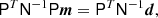
There is an additional complication that arises due to differences in horn A and horn B and the different pixel shapes that are being binned. Differences between the data and the model become exacerbated when one horn is observing a bright source and the other is not. For this reason, we follow the WMAP team’s procedure of asymmetric masking. This entails using a pointing matrix Pam that masks pixel B when pixel A observes a bright spot and pixel B is observing a relatively faint point, and vice versa. We used the same processing mask that is used for LFI to define these bright spots. This gives the modified mapmaking equation:
This form of the mapmaking equation gives an unbiased estimate of the map, while the pixel space covariance matrix is slightly larger due to the data cuts in the asymmetric masking. To solve this equation, we follow Jarosik et al. (2011) and use the stabilized biconjugate gradient method (BiCG-STAB; van der Vorst 1992; Barrett et al. 1994) to solve for this map. We note that we cannot use the usual conjugate gradient algorithm because the matrix  is not symmetric.
Solving Eq. (37) requires iterating over every observation in the TOD and is currently the costliest step in the WMAP analysis pipeline. This typically takes about 20 BiCG iterations, each taking roughly 11 s of wall time or 12 CPU-mins, for a total of about 4 CPU-hrs per sky map. We note that in Table 1, the average time for mapmaking is listed as 6 CPU-hrs. This larger number includes the creation of auxiliary maps (e.g., correlated noise and residual maps) every tenth iteration. The larger figure of 6 CPU-hrs also takes into account the additional variation in the number of samples to reach convergence for a given Gibbs sample. There are several ways to optimize this technique, including using a good initial guess for the map or a well-chosen preconditioner. Although it is not yet implemented in our code, we note that Jarosik et al. (2011) derived the inverse pixel-pixel noise covariance:

Computational resources for end-to-end WMAP Q1-band processing.
and use the central term  evaluated at Nside = 16 as a source for the off-diagonal terms in the preconditioner.
3.4. Noise modeling
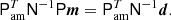
Next, we consider the temporal noise model. The WMAP radiometers have remarkably white noise, with fknee ranging from 0.1–40 mHz, with typical values around 1 mHz (Jarosik et al. 2003). For comparison, the LFI time-ordered data have knee frequencies ranging from 5–200 mHz, with typical values in the 50 mHz region (Ihle et al. 2023). Such long stability periods require more careful analysis in order to characterize the small deviations from white noise in the WMAP data. The WMAP team’s approach was based on a third-order polynomial fit to the two-point temporal correlation function:
![$$ \begin{aligned} N(\Delta t)= {\left\{ \begin{array}{ll} AC&\Delta t=1, \\ \displaystyle {\sum _{n=0}^3} a_n[\log _{10}(|\Delta t|)]^n&1<|\Delta t| < \Delta t_\mathrm{max} , \\ 0&|\Delta t|\ge \Delta t_\mathrm{max} , \end{array}\right.} \end{aligned} $$](/articles/aa/full_html/2023/07/aa43410-22/aa43410-22-eq52.gif)
where AC and an are parameters that were fit to the autocorrelation data, Δt is in units of samples, and Δtmax corresponds to the time lag where the fit crosses zero, typically ∼ 600 s (Jarosik et al. 2007). We convert the parametric noise autocorrelation function4 to a time-domain power spectrum by taking the Fourier transform, 𝒫(f) = [ℱ[N(Δt)]]−1. In contrast, the current LFI-based BEYONDPLANCK noise model is primarily based on a standard 1/f power spectrum density, following Planck Collaboration VI (2014), and Planck Collaboration II (2016, 2020), given in Eq. (4).
Figure 2 shows a comparison of these two noise models in power spectrum domain, compared with one week of Q123 data. Here, we see two main differences. First, the longer stationarity period of one week adopted here allows us to model noise correlations on much longer time scales than the one hour period adopted by WMAP. Second, we see in the inset that the actual WMAP noise spectrum increases at high frequencies, and this is supported by the polynomial-based WMAP approach, but not by the more constrained 1/f noise model. Furthermore, as described by Ihle et al. (2023), the current noise sampler effectively uses the highest frequencies for estimating the white noise level to break a strong degeneracy between fknee and σ0. While this works well for LFI, it is not a good approximation for WMAP; the 1/f model overestimates the noise levels at frequencies f > 0.1 mHz. The recoding effort required to eliminate this bias is easy to describe but nontrivial to implement; essentially, the noise model needs to be augmented with a component proportional to f and the noise PSD sampler needs to fit σ0 jointly with the other parameters, not as a special case.
 |
Fig. 2. Power spectrum for Q123’s week 156, with WMAP’s optimal time-domain filter plotted above. The inset highlights the high frequency region and the need for a non-flat noise model, as originally implemented by the WMAP team. |
However, since the main purpose of the current machinery is to perform joint analysis of many different experiments, it is also necessary to make sure that the new implementation supports other important near-term data sets, and most importantly Planck HFI, which also has strongly colored noise at high frequency. Generalization of the Commander framework to support arbitrary colored noise models will therefore be addressed separately in a future publication. As far as the current work is concerned, the main impact of this shortcoming will be biased time-domain χ2 statistics and slightly overestimated map level uncertainties at intermediate frequencies.
3.5. Sidelobe corrections
The last algorithmic step considered in this paper is far sidelobe corrections. This formalism is identical to the BEYONDPLANCK LFI analysis, as described by Galloway et al. (2023b), and we therefore only give a brief review of the main points here. For a discussion of the corresponding WMAP implementation, we refer to Barnes et al. (2003).
The emission received by a single beam,  , pointing toward the direction
  with a rotation angle ψ may be written as the following convolution,
where s denotes the unpolarized sky signal. As shown by Wandelt & Górski (2001) and Prézeau & Reinecke (2010), this expression may be efficiently computed in harmonic space through the use of fast recurrence relations for the Wigner d-symbols, or, as shown by Galloway et al. (2023b), in terms of spin-weighted spherical harmonics. The main advantage of the latter is the possibility of using highly optimized spherical harmonics libraries for the computationally expensive parts.
In general, b is a full-sky function with a harmonic bandwidth defined by the main beam. However, this is a large and complicated object, and its structure is typically not well characterized outside the main beam. As a result, it is common practice to divide the full beam into (at least) two components, namely, a main beam and far sidelobes. The former is treated at full angular resolution, but limited spatially to just a few degrees around the central axis, while the latter is approximated with a lower resolution grid, but with full 4π coverage (except for the main beam region, which is nulled).
Figure 3 shows the far sidelobe response of the WMAP Q1 radiometer, as estimated by Barnes et al. (2003). In this plot, positive and negative pixels correspond to the A and B sides, respectively. The high resolution regions are measured directly from data, using, for instance, Moon observations, while the low-resolution regions are estimated by model ray tracing and laboratory measurements. The circular holes correspond to the main beam cutouts.
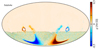 |
Fig. 3. WMAP Q1-band sidelobe map, given in units of relative gain, 4π steradians divided by beam solid angle. |
Following Barnes et al. (2003), we partitioned this map into A and B sides according to positive and negative pixels. To construct the actual sidelobe correction for a given radiometer, we then evaluated Eq. (40) separately for the A and B side radiometers, taking care to evaluate s separately for each detector. That is, the mixing matrices in Eq. (3) are integrated with respect to the bandpass of each individual radiometer. This accounts for possible intensity-to-polarization leakage arising from bandpass differences, which is relevant for the polarized sidelobe corrections.
The issue of spurious polarized signal arising from sidelobes and bandpass differences is treated in Barnes et al. (2003). Given a sidelobe model for two detectors with orthogonal polarization,  and
and  ,
,
the polarized contribution to the sidelobe signal is
![$$ \begin{aligned} \begin{aligned} s^\mathrm{fsl,pol} _t&=[s_{1\mathrm{A} ,t}^\mathrm{fsl} -s_{1\mathrm{B} ,t}^\mathrm{fsl} ] -[s_{2\mathrm{A} ,t}^\mathrm{fsl} -s_{2\mathrm{B} ,t}^\mathrm{fsl} ]. \end{aligned} \end{aligned} $$](/articles/aa/full_html/2023/07/aa43410-22/aa43410-22-eq59.gif)
Given an unpolarized sky, an ideal differential radiometer with identical bandpasses and identical horn transmissions would yield no polarized far sidelobe pickup. Barnes et al. (2003) explicitly models the effect of bandpass mismatch on the spurious polarization signal and constrains its amplitude to be ≲0.4 μK for one year of Q-band data. An additional effect of transmission imbalance can induce a spurious polarization signal:
![$$ \begin{aligned} \begin{aligned} s^\mathrm{fsl,pol} _t&= [(1+x_\mathrm{im,1} )s^\mathrm{fsl} _{1\mathrm{A} ,t}-(1-x_\mathrm{im,1} )s^\mathrm{fsl} _{1\mathrm{B} ,t}] \\&\,-[(1+x_\mathrm{im,2} )s^\mathrm{fsl} _{2\mathrm{A} ,t}-(1-x_\mathrm{im,2} )s^\mathrm{fsl} _{2\mathrm{B} ,t}] \\&=[s_{1\mathrm{A} ,t}^\mathrm{fsl} -s_{1\mathrm{B} ,t}^\mathrm{fsl} ] -[s_{2\mathrm{A} ,t}^\mathrm{fsl} -s_{2\mathrm{B} ,t}^\mathrm{fsl} ] \\&\quad +x_\mathrm{im,1} [s_{1\mathrm{A} ,t}^\mathrm{fsl} +s_{1\mathrm{B} ,t}^\mathrm{fsl} ] -x_\mathrm{im,2} [s_{2\mathrm{A} ,t}^\mathrm{fsl} +s_{2\mathrm{B} ,t}^\mathrm{fsl} ]. \end{aligned} \end{aligned} $$](/articles/aa/full_html/2023/07/aa43410-22/aa43410-22-eq60.gif)
This spurious polarization effect persists when there is no radiometer bandpass mismatch and in this case induces a polarized signal  . In Bennett et al. (2013), Q11 and Q12 have transmission imbalance parameters of:

whereas our analysis has values of


The difference between the imbalance parameters xim, 1 − xim, 2 is consistent between both treatments, suggesting that the imbalance-induced sidelobe polarization signal is also present in the WMAP timestreams. The effect of transmission imbalance on sidelobes is not mentioned in Barnes et al. (2003). This accounts for the main difference between the polarized sidelobe estimate in this work and that of Barnes et al. (2003).
Figure 4 shows the Q1-band temperature-to-polarization leakage sidelobe signal separately for bandpass mismatch (top row) and transmission imbalance (bottom row). Here, we see that the transmission imbalance contribution is about one order of magnitude larger than the bandpass mismatch contribution and it has a very distinct morphology. This morphology is very similar to the imbalance modes described in Sect. 3.5.1 of Jarosik et al. (2007), which we reproduce in Fig. 5.
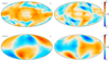 |
Fig. 4. Estimates of WMAP Q1-band polarized sidelobe pickup. We note the differing dynamic ranges for each panel. Top: Commander estimate of the polarized sidelobe pickup, taking into account only the bandpass differences between each channel. Bottom: Commander estimate of the polarized sidelobe pickup, taking into account only the transmission imbalance parameters. |
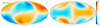 |
Fig. 5. Official WMAP Q-band imbalance template. We note that the units are arbitrary, as this is an eigenmode to be downweighted in the low-resolution likelihood analysis. |
The similarity between the imbalance mode and the polarized sidelobe signal is worth exploring in further detail. The two signals come from different effects. The imbalance template was generated by evaluating the mapmaking procedure assuming a 10% increase and a 10% decrease in the two imbalance parameters, and is thus generated by small deviations from the true underlying imbalance parameters. Conversely, the polarized sidelobe signal persists even if the imbalance parameters are estimated, as long as x1 ≠ x2.
This can be partially explained by the total convolution formalism described in Galloway et al. (2023b). Assuming that we are convolving a beam with spherical harmonic representation bℓmb with a sky signal sℓms dominated by the ℓ = 1 mode, i.e., the Solar dipole, the signal as a function of beam orientation is given by:
This means that the sidelobe pickup will mainly be determined by the ℓ = 1 modes of the beam, hence, adding a large contribution that is modulated by the boresight angle ψ. Conversely, incorrect imbalance templates for a pencil beam will induce extra signal pickup from the Solar dipole that depends only on the orientation of the spacecraft. Essentially, the signals look so similar because they are both dominated by observing the Solar dipole with similar orientations. At the same time, this explains the small differences between the two effects. The two signals are masked in the timestream at different times, since the processing mask depends on the pointing of the main beam. This explains why the signal is not straight along the prime meridian in the sidelobe imbalance signal and why the notches above and below the Galactic anticenter in U are of opposite signs between the two maps.
The main differences between the Commander and the WMAP sidelobe modeling presented by Barnes et al. (2003), are the following: (1) Barnes et al. (2003) used a smaller transition radius between main beam and sidelobe of  than the final nine-year WMAP and the current analysis, both of which use
  (Hill et al. 2009; Bennett et al. 2013). This causes a significant reduction of pickup that in later releases is included in the main beam. (2) Barnes et al. (2003) generated sidelobe templates using the first-year scan pattern convolved with the first-year estimate of the sky map, whereas our analysis uses the full nine-year scan strategy convolved with the parametric sky model ssky(ν, a, β), which has been fit to the WMAP9+Haslam+LFI+Planck 353/857 GHz sky maps. 3) Barnes et al. (2003) explicitly took into account the polarized sidelobe pickup from polarized sky signal using the full antenna gain G(n) and the polarization direction perpendicular to the sky, P(n). Only the gain amplitude is reported on LAMBDA5, so we are unable to account for the intrinsically polarized pickup of the sidelobes. 4) Temperature-to-polarization leakage from transmission imbalance is included in the Commander model, but is not mentioned by Barnes et al. (2003).
From the individual radiometer sidelobe corrections, we form an effective correction per DA in the time domain,  , weighting each timestream by the respective transmission imbalance factors, as outlined in Eq. (25). This function is then subtracted from the calibrated TOD residual in Eq. (28) prior to mapmaking. Alternatively, the entire residual may be replaced by
  , in which case the resulting map will be an image of the net sidelobe correction in the map domain. Both variations are considered in the next section.
As a consistency check, we developed an alternate python pipeline for simulating sidelobe timestreams and mapmaking6. We used the ducc7 implementation of totalconvolver (Wandelt & Górski 2001; Prézeau & Reinecke 2010) to simulate the WMAP sidelobe contribution from a pure Solar dipole reported by Jarosik et al. (2011), with amplitude 3355 μK and direction  and the two horns’ orientations. We use the transmission imbalance parameters reported in Bennett et al. (2013) to simulate observed timestreams, then bin the maps at Nside = 16 and solve for the output map exactly using the scipy sparse linear algebra package (Virtanen et al. 2020). This python implementation of the mapmaker and simulated timestreams reproduces a low resolution version of maps obtained using Commander’s iterative solver.
3.6. Differences between the Cosmoglobe and WMAP pipelines
Although our goal is not a reproduction of the WMAP mapmaking pipeline, we have in general attempted to follow the WMAP team’s approach. There are some algorithmic differences that can result in different frequency maps derived from the same time-ordered data. The differences we are aware of include the following.
Calibration. The WMAP team developed a physical model for the gain of the instrument as a function of housekeeping parameters. These parameters were fit to the hourly gain estimates using the CMB dipole as a calibration source. The nine-year best-fit parameters are given in Appendix A of Greason et al. (2012). In contrast, the Commander framework calibrates the time-ordered data on a weekly cadence by comparing directly to the expected sky amplitude, and most importantly to the orbital and Solar CMB dipoles; for full details, see Gjerløw et al. (2023). The Commander approach makes fewer assumptions regarding the physical origin of gain fluctuations, but stronger assumptions regarding their stability in time.
Transmission imbalance. As discussed by Jarosik et al. (2003, 2007), the WMAP team derived transmission imbalance parameters using ten precession periods at a time and estimated a corresponding uncertainty through the variation during the mission. This quantity is also dependent on the treatment of low-frequency noise, thus, the original algorithm solved for a cubic polynomial in each period while fitting for the transmission imbalance coefficients. The resulting transmission imbalance templates were projected out from low-resolution noise covariance matrices to account for their effect on cosmological parameters. In contrast, the current analysis assumes a constant imbalance parameter for the entire mission, but allows it to vary in each Gibbs iteration, and thereby marginalizing over this parameter directly in the data model in a way that is fully analogous to the gain (Gjerløw et al. 2023). We applied no explicit postproduction corrections to any data product for transmission imbalance.
Baseline evaluation. The raw WMAP data have a large offset from zero. This is treated explicitly as a time-varying constant within each stationary period in the official pipeline, but as an offset in the correlated noise component in the Commander framework. In the picture where baseline and correlated noise are treated as separate terms, there is a correlation between gain, baseline, and 1/f noise, as discussed in Hinshaw et al. (2003). To address this, the WMAP team applied a whitening filter using an estimate of the 1/f noise spectrum, and iteratively solved for the baseline. In contrast, we fit a linear baseline per weeklong scan in the Commander pipeline, and residual baseline fluctuations are absorbed by the ncorr sampling (Ihle et al. 2023).
Solar dipole. While the WMAP team subtracted an estimate of the Solar dipole from the time-ordered data before mapmaking, resulting in dipole-free frequency maps (Hinshaw et al. 2003), Commander retains it for calibration and component separation purposes, following Planck DR4 (Planck Collaboration Int LVII 2020; Gjerløw et al. 2023; Andersen et al. 2023).
Mapmaking. The WMAP team accounted for correlated noise weighting by estimating a two-point correlation function in time-domain and used this to pre-whiten the TOD prior to mapmaking. In contrast, we assumed a 1/f noise model and sampled correlated noise explicitly as a stochastic field in time-domain (Ihle et al. 2023). We note again that this noise PSD model will be generalized in the future to fully capture the temporal behaviour of the WMAP noise, as discussed in Sect. 3.4.
Bandpass corrections. The WMAP team suppressed temperature-to-polarization leakage from bandpass differences between radiometers by solving for a spurious map, S, per radiometer. In contrast, we use a parametric foreground model to subtract these bandpass effects in time-domain (Svalheim et al. 2023). The main advantage of the latter is that it requires fewer free parameters and therefore results in a lower degree of white noise, while the main disadvantage is a stronger sensitivity to the foreground model. We find that the two approaches perform similarly.
4. Results
We are now ready to present the results obtained by applying the methods outlined in Sects. 2 and 3 to the WMAP Q1-band data. We have made all data, code, and parameter files required to perform this analysis publicly available in the Commander source code8.
We emphasize that the results presented below are a simplified version of the more complete Gibbs sampling problem. Similar to the WMAP9 analysis, we calibrate the raw data to a fixed signal and adjust the gain parameters and noise model while correcting for known instrumental effects. Our analysis differs from the WMAP9 processing in that we calibrate to the total sky model rather than just the orbital dipole. The analysis choice to enforce a single sky model across all sky maps is the primary advantage of the Commander method, by design reducing degeneracies due to observing strategy. A complete Commander analysis, jointly analyzing the time-ordered data of both Planck LFI and WMAP, while fitting for the sky parameters, will fully leverage the power of this method.
4.1. Computational resources
The first main goal of the current paper is to quantify the computational resources that will be required for a future full end-to-end WMAP analysis. Most of our efforts have been spent on implementing the main new analysis steps, rather than optimizing for speed. Examples of known optimizations left for future work include using optimal lengths for fast Fourier transform evaluations (Galloway et al. 2023a), implementing a more effective preconditioner for mapmaking (Bennett et al. 2013) and improving load balancing for parallelization. With these caveats in mind, in Table 1, we summarize the computational expenses required to run the Q1-band analysis on a computer system with 64 AMD EPYC3 7543 2.8 GHz cores, using the Intel Parallel Studio XE 20.0.4.912 Fortran compiler. The processing times listed include the integrated time including each parallel core. To obtain the cost in wall time, the cost must be divided by the number of cores used, in this case 64.
The total cost per full Gibbs sample is 22 CPU-hrs, which is comparable to the Planck LFI 44 GHz channel cost of 17 CPU-hrs (Galloway et al. 2023a). This is despite the fact that the compressed Q-band data volume is only 8% of the 44 GHz and all time-domain operations are correspondingly faster. The explanation is the more expensive differential mapmaker; approximately a quarter of the total WMAP analysis time is spent in the mapmaking procedure, evaluating the matrix operation  . For comparison, map binning for the LFI 44 GHz channel accounts for less than 3% of its total run time. Thus, the differential mapmaking procedure is the main additional step in the WMAP analysis and all other processing steps scale with 𝒪(N log N), due to the use of FFTs in the calibration steps. Better preconditioning is a priority for optimizing the current code. Based on a conservative 𝒪(N log N) scaling, we expect the cost for each band to be 20, 20, 30, 40, and 72 CPU hrs for each K, Ka, Q, V, and W DA, respectively.
The memory requirement for storing the Q1-band data is only 14 GB, reduction of the uncompressed 76 GB data by a factor of four. The full WMAP data volume only corresponds to 20% of the LFI data volume, which can be considered an incremental increase. Based both on memory and CPU requirements, we conclude that a future Bayesian end-to-end WMAP analysis is well within the reach of current computer systems, both as a standalone analysis and as a joint WMAP–LFI analysis.
4.2. Temperature map quality assessment
We now turn to the quality of the maps, starting with the temperature component. The top panel in Fig. 6 shows the Commander-derived Q1-band sky map (after subtracting the Solar CMB dipole), the second panel shows the corresponding official WMAP9 sky map (Bennett et al. 2013), and the third panel shows their difference. Overall, we see that the two maps are consistent at the ∼2.5 μK level with several systematic features, of which the most salient is a quadrupole aligned with the Solar dipole.
 |
Fig. 6. Q1-band temperature results. Top panel: CommanderQ1-band temperature map. Second panel: corresponding official WMAP sky map. Third panel: straight difference between Commander and WMAP. Fourth panel: single Commander TOD residual sample. Bottom panel: single Commander correlated noise sample. |
This signal does not appear in either the Commander TOD residual map (created by binning d − stot − ncorr into a sky map; fourth panel in Fig. 6), or the correlated noise map (bottom panel). Together, these two maps act as a “trash can” in the Commander processing framework in the sense that they highlight any signal in the raw data that cannot be accommodated by any of the other components. The main structure in the residual and ncorr maps is correlated with the Galactic plane, indicating an inadequate sky model. An improved sky model will be obtained during a future joint TOD analysis between the Planck LFI data and the WMAP K–V-band data. With the K-band map included (as opposed to being excluded as in BeyondPlanck Collaboration 2023), there will also be an opportunity to improve the low-frequency foreground model by, for example, including a more sophisticated synchrotron model than a simple power law.
We have two hypotheses for the source of the quadrupolar difference between the WMAP and COSMOGLOBE map. One potential explanation is the 1.2 μK kinematic quadrupole, which is not removed in the WMAP analysis (Jarosik et al. 2007; Larson et al. 2015) but is indeed in the BEYONDPLANCK framework (BeyondPlanck Collaboration 2023). Another potential contributor to the residual is different treatments of the Solar dipole. The WMAP estimate of the Solar dipole 3.359 ± 0.008 mK (Hinshaw et al. 2009), is removed directly in the timestream rather than projecting to the map space and removing, as in the Commander framework. Our Q1-band amplitude of 3.358 mK is consistent with the official WMAP results, although we note that since the sky signal is fixed, this is an incomplete comparison.
We reproduce the Q-band intensity sidelobe in Fig. 7, and compare with the dipole-subtracted sidelobe prediction in the bottom panel. The amplitude and morphology of the two computations are very similar, except for the holes in point sources around the Galactic plane. This is due to both the different amounts of data used in the two, one, and nine years, respectively, and to the different sidelobe cutoff radii in both sidelobe maps,  and
and  , respectively9.
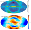 |
Fig. 7. Temperature sidelobe predictions. Top: WMAP estimate of the temperature sidelobe correction; reproduction from Barnes et al. (2003). Bottom: Commander estimate of the temperature sidelobe correction, after an overall dipole is removed. |
4.3. Polarization map quality assessment
We now turn our attention to the polarization sky maps. As in Fig. 6, for the temperature, the top panel of Fig. 8 shows the CommanderQ1-band Stokes Q and U maps; the middle panel shows the corresponding official WMAP sky map; and the bottom panel shows their difference. We see that the Galactic plane is in this case almost perfectly consistent between the two pipelines, but there is also a distinct large-scale pattern present at high Galactic latitudes with a morphology similar to the signal that the WMAP team identified as poorly measured modes in the mapmaking procedure, which can be seen in the WMAP official imbalance templates shown in Fig. 5. This structure was identified in Sect. 3.5.1 of Jarosik et al. (2007) as the coupling of the dipole signal with small errors in the transmission imbalance parameters. However, as discussed in Sect. 3.5, a major novel result from the current analysis is that a nearly identical morphology may be reproduced deterministically in terms of temperature-to-polarization leakage arising from the three-way coupling between the CMB Solar dipole, transmission imbalance, and sidelobe pickup.
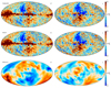 |
Fig. 8. Q1-band polarization maps. Top: CommanderQ1-band polarization map, smoothed to 2° FWHM. Middle: corresponding official WMAP Q1-band sky map, also smoothed to 2° FWHM. Bottom: Commander solution minus WMAP solution, smoothed to 10° FWHM. |
In particular, Fig. 4 shows the polarized sidelobe predicted by Commander, using the model described in Sect. 3.5. We note that the amplitude of the polarized sidelobe predicted by Commander is an order of magnitude smaller than the large scale feature difference feature. The amplitude difference may be caused by the sidelobe itself or the magnitude of the transmission imbalance factors. This implies that the polarized sidelobe as described here can at best only partially explain the difference between the Commander and WMAP9 maps.
Next, we want to understand whether the residual pattern in the bottom panel of Fig. 8 is present in the Commander or WMAP maps, or both. To this aim, Fig. 9 shows differences between the WMAP K-band channel and the WMAP (top) and Commander (bottom) Q1-band maps, in which polarized synchrotron emission is greatly suppressed. In both cases, the K-band map has been scaled with a factor of 0.17 prior to subtraction, to account for the different central frequencies of the two channels, equivalent to assuming a synchrotron spectral index of βs = −3.1. In these plots, we see that the sidelobe pattern is present in the official WMAP Q1-band map, while it is much weaker in the Commander map. This implies that Commander is able to remove the imbalance modes accurately without the need of a post-production modification.
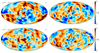 |
Fig. 9. Difference maps between WMAP K-band and WMAP (top row) and Commander (bottom row) Q1-band, designed to reduce polarized synchrotron emission. The K-band map has been scaled by a factor of 0.17 to account for the different central frequencies of the two frequency channels. |
The only possible location for the imbalance modes in the Commander data model is in the correlated noise, which we display a map of, along with the TOD residuals in Fig. 10. Here, we see large-scale structures with a similar amplitude to the imbalance modes in WMAP. The imbalance mode and polarized sidelobe are accounted for in the correlated noise component for Commander, resulting in broad features modulated by the scanning strategy. Ideally, this should look like stochastic, “stripy” noise (see, e.g., Basyrov et al. 2023, for an LFI example), but this map is both systematic and inconsistent with the 1/f correlated noise model. The reason for why this signal does not end up in the actual frequency sky map is that we assume the sky model to be defined by the Planck- and LFI-based BEYONDPLANCK model, which provides the necessary leverage to extract the current signal. We could find no compelling evidence for the imbalance modes being present in the correlated noise map at the 2.5 μK. However, preliminary runs of the other DAs have have this signature in the correlated noise level at a higher level, so we do not yet rule out the imbalance modes being absorbed into the Q1 DA’s correlated noise.
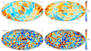 |
Fig. 10. Q1-band polarized deviations from the data model. Top row: Commander correlated noise sample for the Q1 channel in polarization smoothed with 5deg FWHM. Bottom row: corresponding TOD residual sample, also smoothed with a 5deg FWHM beam. |
As a final test of our method, we directly compared the polarized Q1 and Q2-band data. The two DAs have overlapping bandpasses, with effective frequencies of 40.72 GHz and 40.51 GHz, respectively (Bennett et al. 2013). Several other instrumental properties, such as the knee frequencies, gain, and beam orientation, vary between the two DAs. Properly treated, the maps derived from these DAs should be consistent with each other, save for instrumental noise fluctuations. At the same time, the consistency of the WMAP-processed Q DAs compared with the Commander-processed Q DAs highlights the differences between our two approaches.
Figure 11 shows the polarized half-difference maps, (Q1 − Q2)/2, for the Q and U Stokes parameters. As expected, the WMAP half-difference maps are visually dominated by the poorly measured imbalance modes. As explained in Jarosik et al. (2007), this is mainly a large-scale phenomenon that is downweighted in the low-resolution likelihood analysis. Conversely, the Commander half-difference maps are consistent at the 2.5 μK level without any post-processing. This agreement is partially due to conditioning the data on the sky model, so that correlated noise accounts for the deviations from the sky model. Ideally, the WMAP approach of downweighting imbalance modes in the likelihood should be mathematically equivalent to the Commander approach of drawing random samples of these modes to marginalize over them.
 |
Fig. 11. Half-difference maps (Q1 − Q2)/2, smoothed to 5°. Top row: WMAP half-difference map. Bottom row: Commander half-difference map. |
5. Summary and conclusions
This paper has two main goals. The first goal is to assess whether a full Bayesian end-to-end BEYONDPLANCK-style analysis of the WMAP data is technically feasible and, if so, how expensive it would be. Based on the results presented here, we can conclude affirmatively, as the current computational cost is 44 CPU-hrs per full Q1-band Gibbs sample. This is comparable to the cost of the Planck LFI 44 GHz channel and is thus well within the reach of current computers. Furthermore, this estimate is an upper limit, as the current WMAP module has not yet been heavily optimized and, in particular, a new BiCG-STAB preconditioner may result in a significant speedup. We have also found that the amount of recoding effort required to generalize the existing Commander machinery to a new data set is fully manageable; in this specific case, it corresponds to 𝒪(1) postdoc years, starting from no working knowledge of either the WMAP or Commander pipelines.
The second goal was to assess the quality of the maps and whether the current code is ready for production work. In this case, we conclude with a tentatively positive answer. The remaining work either consists of optimization (e.g., better preconditioning in mapmaking, sidelobe interpolation speedups) or improving suboptimal data treatment (e.g., proper baseline fitting, expanded PSD model). Indeed, our preliminary work comparing the WMAP Q1 and Q2 sky maps suggests that the software is quickly reaching a level of maturity at which a joint Planck LFI/WMAP analysis may be performed.
Considering the new results presented in this paper, sidelobe contamination in general has taken on a new importance with respect to the publicly available WMAP large-scale polarization data. Although the polarized sidelobe pattern is morphologically very similar to the imbalance modes, its contribution is not explicitly undergoing marginalization in the low-resolution covariance matrices used for low-ℓ CMB likelihood estimation (Hinshaw et al. 2013); therefore, it can directly bias estimates of, for instance, the reionization optical depth derived from WMAP polarization data, at a level of 𝒪(0.5 μK). The potential sidelobe contamination is an important issue for future joint analyses of WMAP and Planck data, which currently use pre-pixelized sky maps as in the BEYONDPLANCK analysis; a nonnegligible fraction of the Planck–WMAP residuals reported by Planck Collaboration IV (2020) and BeyondPlanck Collaboration (2023) may be due to this specific issue.
We argue that the main takeaway from this work is another illustration of the importance of joint multi-experiment analysis. As amply illustrated through both the WMAP and Planck analysis efforts, any given experiment has blind spots to which it is not sensitive. These blind spots lead to unconstrained modes in the frequency maps, which, in turn, may bias both astrophysical and cosmological conclusions. We argue that the optimal solution to this problem is not primarily more clever algorithms (even though such can certainly can help), but rather adding more data. Whenever a given degeneracy limits the data analysis, whether it is foreground uncertainties caused by a limited frequency range or unconstrained map modes caused by the scanning strategy, the best solution is to bring in more data to break the degeneracy. This is the goal of the COSMOGLOBE project; to jointly analyze the world’s best data. This paper is an important step in that direction, aiming to combine the world’s two best CMB satellite data sets within one joint framework.
The initial version of this work had a difference between the WMAP final sky map and the sky map in this reanalysis that was morphologically identical to the WMAP sidelobe as computed by Barnes et al. (2003). We have since determined that we oriented the beam incorrectly. We have corrected this by rotating by 135° before convolving with the sky model.
Acknowledgments
We thank Prof. Charles Bennett, Dr. Janet Weiland, Prof. Lyman Page, and Dr. Zhilei Xu for useful comments and suggestions that improved this work. We thank the anonymous referee whose suggestions improved this paper. We thank Prof. Pedro Ferreira and Dr. Charles Lawrence for useful suggestions, comments and discussions. We also thank the entire Planck and WMAP teams for invaluable support and discussions, and for their dedicated efforts through several decades without which this work would not be possible. The current work has received funding from the European Union’s Horizon 2020 research and innovation programme under grant agreement numbers 776282 (COMPET-4; BEYONDPLANCK), 772253 (ERC; BITS2COSMOLOGY), and 819478 (ERC; COSMOGLOBE). In addition, the collaboration acknowledges support from ESA; ASI and INAF (Italy); NASA and DoE (USA); Tekes, Academy of Finland (grant no. 295113), CSC, and Magnus Ehrnrooth foundation (Finland); RCN (Norway; grant nos. 263011, 274990); and PRACE (EU). We acknowledge the use of the Legacy Archive for Microwave Background Data Analysis (LAMBDA), part of the High Energy Astrophysics Science Archive Center (HEASARC). HEASARC/LAMBDA is a service of the Astrophysics Science Division at the NASA Goddard Space Flight Center.
References
- Andersen, K. J., Aurlien, R., Banerji, R., et al. 2023, A&A, 675, A13 (BeyondPlanck SI) [NASA ADS] [CrossRef] [EDP Sciences] [Google Scholar]
- Barnes, C., Hill, R. S., Hinshaw, G., et al. 2003, ApJS, 148, 51 [NASA ADS] [CrossRef] [Google Scholar]
- Barrett, R., Berry, M. W., Chan, T. F., et al. 1994, Templates for the Solution of Linear Systems (Society for Industrial and Applied Mathematics) [Google Scholar]
- Basyrov, A., Suur-Uski, A.-S., Colombo, L. P. L., et al. 2023, A&A, 675, A10 (BeyondPlanck SI) [NASA ADS] [CrossRef] [EDP Sciences] [Google Scholar]
- Bennett, C. L., Bay, M., Halpern, M., et al. 2003a, ApJ, 583, 1 [NASA ADS] [CrossRef] [Google Scholar]
- Bennett, C. L., Halpern, M., Hinshaw, G., et al. 2003b, ApJS, 148, 1 [Google Scholar]
- Bennett, C. L., Larson, D., Weiland, J. L., et al. 2013, ApJS, 208, 20 [Google Scholar]
- BeyondPlanck Collaboration (Andersen, K. J., et al.) 2023, A&A, 675, A1 (BeyondPlanck SI) [Google Scholar]
- Fixsen, D. J. 2009, ApJ, 707, 916 [Google Scholar]
- Galloway, M., Andersen, K. J., Aurlien, R., et al. 2023a, A&A, 675, A3 (BeyondPlanck SI) [NASA ADS] [CrossRef] [EDP Sciences] [Google Scholar]
- Galloway, M., Reinecke, M., Andersen, K. J., et al. 2023b, A&A, 675, A8 (BeyondPlanck SI) [NASA ADS] [CrossRef] [EDP Sciences] [Google Scholar]
- Gelman, A., & Rubin, D. B. 1992, Statist. Sci., 7, 457 [NASA ADS] [Google Scholar]
- Gjerløw, E., Ihle, H. T., Galeotta, S., et al. 2023, A&A, 675, A7 (BeyondPlanck SI) [NASA ADS] [CrossRef] [EDP Sciences] [Google Scholar]
- Greason, M. R., Limon, M., Wollack, E., et al. 2012, Nine-Year Explanatory Supplement, 5th edn. (Greenbelt, MD: NASA/GSFC) [Google Scholar]
- Haslam, C. G. T., Salter, C. J., Stoffel, H., & Wilson, W. E. 1982, A&AS, 47, 1 [NASA ADS] [Google Scholar]
- Hauser, M. G., Arendt, R. G., Kelsall, T., et al. 1998, ApJ, 508, 25 [Google Scholar]
- Hill, R. S., Weiland, J. L., Odegard, N., et al. 2009, ApJS, 180, 246 [NASA ADS] [CrossRef] [Google Scholar]
- Hinshaw, G., Barnes, C., Bennett, C. L., et al. 2003, ApJS, 148, 63 [NASA ADS] [CrossRef] [Google Scholar]
- Hinshaw, G., Weiland, J. L., Hill, R. S., et al. 2009, ApJS, 180, 225 [Google Scholar]
- Hinshaw, G., Larson, D., Komatsu, E., et al. 2013, ApJS, 208, 19 [Google Scholar]
- Ihle, H. T., Bersanelli, M., Franceschet, C., et al. 2023, A&A, 675, A6 (BeyondPlanck SI) [NASA ADS] [CrossRef] [EDP Sciences] [Google Scholar]
- Jarosik, N., Barnes, C., Bennett, C. L., et al. 2003, ApJS, 148, 29 [NASA ADS] [CrossRef] [Google Scholar]
- Jarosik, N., Barnes, C., Greason, M. R., et al. 2007, ApJS, 170, 263 [NASA ADS] [CrossRef] [Google Scholar]
- Jarosik, N., Bennett, C. L., Dunkley, J., et al. 2011, ApJS, 192, 14 [Google Scholar]
- Kamionkowski, M., & Kovetz, E. D. 2016, ARA&A, 54, 227 [NASA ADS] [CrossRef] [Google Scholar]
- Kelsall, T., Weiland, J. L., Franz, B. A., et al. 1998, ApJ, 508, 44 [Google Scholar]
- Larson, D., Weiland, J. L., Hinshaw, G., & Bennett, C. L. 2015, ApJ, 801, 9 [NASA ADS] [CrossRef] [Google Scholar]
- Mather, J. C., Cheng, E. S., Cottingham, D. A., et al. 1994, ApJ, 420, 439 [Google Scholar]
- Page, L., Hinshaw, G., Komatsu, E., et al. 2007, ApJS, 170, 335 [Google Scholar]
- Penzias, A. A., & Wilson, R. W. 1965, ApJ, 142, 419 [CrossRef] [Google Scholar]
- Planck Collaboration I. 2014, A&A, 571, A1 [NASA ADS] [CrossRef] [EDP Sciences] [Google Scholar]
- Planck Collaboration VI. 2014, A&A, 571, A6 [NASA ADS] [CrossRef] [EDP Sciences] [Google Scholar]
- Planck Collaboration IX. 2014, A&A, 571, A9 [NASA ADS] [CrossRef] [EDP Sciences] [Google Scholar]
- Planck Collaboration XIV. 2014, A&A, 571, A14 [NASA ADS] [CrossRef] [EDP Sciences] [Google Scholar]
- Planck Collaboration II. 2016, A&A, 594, A2 [NASA ADS] [CrossRef] [EDP Sciences] [Google Scholar]
- Planck Collaboration X. 2016, A&A, 594, A10 [NASA ADS] [CrossRef] [EDP Sciences] [Google Scholar]
- Planck Collaboration I. 2020, A&A, 641, A1 [NASA ADS] [CrossRef] [EDP Sciences] [Google Scholar]
- Planck Collaboration II. 2020, A&A, 641, A2 [NASA ADS] [CrossRef] [EDP Sciences] [Google Scholar]
- Planck Collaboration IV. 2020, A&A, 641, A4 [NASA ADS] [CrossRef] [EDP Sciences] [Google Scholar]
- Planck Collaboration V. 2020, A&A, 641, A5 [NASA ADS] [CrossRef] [EDP Sciences] [Google Scholar]
- Planck Collaboration Int LVII. 2020, A&A, 643, A42 [NASA ADS] [CrossRef] [EDP Sciences] [Google Scholar]
- Prézeau, G., & Reinecke, M. 2010, ApJS, 190, 267 [CrossRef] [Google Scholar]
- Remazeilles, M., Dickinson, C., Banday, A. J., Bigot-Sazy, M.-A., & Ghosh, T. 2015, MNRAS, 451, 4311 [Google Scholar]
- Smoot, G. F., Bennett, C. L., Kogut, A., et al. 1992, ApJ, 396, L1 [Google Scholar]
- Svalheim, T. L., Zonca, A., Andersen, K. J., et al. 2023, A&A, 675, A9 (BeyondPlanck SI) [NASA ADS] [CrossRef] [EDP Sciences] [Google Scholar]
- van der Vorst, H. A. 1992, SIAM J. Sci. Stat. Comput., 13, 631 [CrossRef] [Google Scholar]
- Virtanen, P., Gommers, R., Oliphant, T. E., et al. 2020, Nat. Methods, 17, 261 [Google Scholar]
- Wandelt, B. D., & Górski, K. M. 2001, Phys. Rev. D, 63, 12300 [NASA ADS] [CrossRef] [Google Scholar]
All Tables
All Figures
|
Fig. 1. Sample of WMAP TOD. This Q113 datastream was recorded on July 7, 2003. At this resolution, the discreteness of the digital units is apparent, a property which makes these data highly compressible. |
| In the text | |
|
Fig. 2. Power spectrum for Q123’s week 156, with WMAP’s optimal time-domain filter plotted above. The inset highlights the high frequency region and the need for a non-flat noise model, as originally implemented by the WMAP team. |
| In the text | |
|
Fig. 3. WMAP Q1-band sidelobe map, given in units of relative gain, 4π steradians divided by beam solid angle. |
| In the text | |
|
Fig. 4. Estimates of WMAP Q1-band polarized sidelobe pickup. We note the differing dynamic ranges for each panel. Top: Commander estimate of the polarized sidelobe pickup, taking into account only the bandpass differences between each channel. Bottom: Commander estimate of the polarized sidelobe pickup, taking into account only the transmission imbalance parameters. |
| In the text | |
|
Fig. 5. Official WMAP Q-band imbalance template. We note that the units are arbitrary, as this is an eigenmode to be downweighted in the low-resolution likelihood analysis. |
| In the text | |
|
Fig. 6. Q1-band temperature results. Top panel: CommanderQ1-band temperature map. Second panel: corresponding official WMAP sky map. Third panel: straight difference between Commander and WMAP. Fourth panel: single Commander TOD residual sample. Bottom panel: single Commander correlated noise sample. |
| In the text | |
|
Fig. 7. Temperature sidelobe predictions. Top: WMAP estimate of the temperature sidelobe correction; reproduction from Barnes et al. (2003). Bottom: Commander estimate of the temperature sidelobe correction, after an overall dipole is removed. |
| In the text | |
|
Fig. 8. Q1-band polarization maps. Top: CommanderQ1-band polarization map, smoothed to 2° FWHM. Middle: corresponding official WMAP Q1-band sky map, also smoothed to 2° FWHM. Bottom: Commander solution minus WMAP solution, smoothed to 10° FWHM. |
| In the text | |
|
Fig. 9. Difference maps between WMAP K-band and WMAP (top row) and Commander (bottom row) Q1-band, designed to reduce polarized synchrotron emission. The K-band map has been scaled by a factor of 0.17 to account for the different central frequencies of the two frequency channels. |
| In the text | |
|
Fig. 10. Q1-band polarized deviations from the data model. Top row: Commander correlated noise sample for the Q1 channel in polarization smoothed with 5deg FWHM. Bottom row: corresponding TOD residual sample, also smoothed with a 5deg FWHM beam. |
| In the text | |
|
Fig. 11. Half-difference maps (Q1 − Q2)/2, smoothed to 5°. Top row: WMAP half-difference map. Bottom row: Commander half-difference map. |
| In the text | |
Current usage metrics show cumulative count of Article Views (full-text article views including HTML views, PDF and ePub downloads, according to the available data) and Abstracts Views on Vision4Press platform.
Data correspond to usage on the plateform after 2015. The current usage metrics is available 48-96 hours after online publication and is updated daily on week days.
Initial download of the metrics may take a while.