| Issue |
A&A
Volume 656, December 2021
|
|
|---|---|---|
| Article Number | A120 | |
| Number of page(s) | 15 | |
| Section | The Sun and the Heliosphere | |
| DOI | https://doi.org/10.1051/0004-6361/202142028 | |
| Published online | 10 December 2021 | |
Forward modelling of heating within a coronal arcade
1
School of Mathematics and Statistics, University of St. Andrews, St. Andrews, Fife KY16 9SS, UK
e-mail: This email address is being protected from spambots. You need JavaScript enabled to view it.
2
Rosseland Centre for Solar Physics, University of Oslo, PO Box 1029 Blindern 0315 Oslo, Norway
Received:
16
August
2021
Accepted:
25
October
2021
Abstract
Aims. We investigate the synthetic observational signatures generated from numerical models of coronal heating in an arcade in order to determine what features are associated with such heating and what tools can be used to identify them.
Methods. We consider two simulations of coronal arcades driven by footpoint motions with different characteristic timescales. Forward modelling is then conducted, and the synthetic emission data are analysed (e.g., intensities, Doppler shifts, line widths and estimated kinetic energies).
Results. The total intensity and Doppler shift perturbations clearly show the magnetic structure of the coronal arcade. Contrasts in the local Doppler velocity also highlight the locations of separatrix surfaces. The distinguishing feature of the models with short and long timescale photospheric motions (in comparison to the Alfvén travel time along a loop) is that of the frequencies. Through fast Fourier transform analysis of the Doppler velocities, it is clear that when short timescale footpoint motions are present, higher frequency perturbations are observed. For longer timescale footpoint motions, the dominant signal is that of lower frequencies; however, higher (but less powerful) frequencies were also detected, which matched the natural Alfvén frequency of the background magnetic field. Signatures of Alfvénic waves were identified in both models, with fast wave signatures observable when short timescale driving is present. Finally, we examine the estimates of the kinetic energy using the Doppler velocities and find it to be significantly underestimated within these models.
Conclusions. All of the observables within this article behave as one would expect, given the evolution of the plasma parameters. Such features were, for example, Alfvén waves, fast waves, the arcade structure and separatrix surfaces. We were able to differentiate between the two models by examining the frequencies present. The Doppler velocities cannot provide accurate estimates of the total kinetic energy or even the component parallel to the line-of-sight (LOS). This is due to some of the plasma being outside the formation temperature of the ion, the multi-directional driver limiting the proportion of the velocity aligned along the LOS, and cancellation of the velocity along the LOS. The exact impact each factor has on the estimation is dependent on the setup of the model and the emission line under investigation.
Key words: Sun: corona / Sun: magnetic fields / Sun: oscillations / magnetohydrodynamics (MHD)
© ESO 2021
1. Introduction
It is well established that the solar corona is heated up to millions of degrees. In order to investigate the source of this heating, various models that could generate such high temperatures have been suggested. Coronal heating theories can be found in reviews by, for example, Walsh & Ireland (2003), Klimchuk (2006), Klimchuk (2015), Parnell & De Moortel (2012), and De Moortel & Browning (2015). Convective motions at the Sun’s surface are thought to be the source of energy required to heat the solar corona. Energy flux is injected into the solar atmosphere due to these photospheric motions and is subsequently converted into heat. However, how and where this energy is released is still unclear.
The models proposed for the release of energy into the solar corona largely fall into two broad groups: AC heating and DC heating. These two categories differ according to the timescale of the photospheric motions that drive them. When timescales are short (in comparison to the Alfvén travel time along a coronal loop), we are in the AC heating regime. On the other hand, if the driving timescale is long, we are in the DC heating regime. In either case, in order to obtain any significant energy release, small scales need to be generated within the magnetic and/or velocity fields. For comprehensive coronal heating reviews, we direct the reader to Parnell & De Moortel (2012), Arregui (2015), De Moortel & Browning (2015), Klimchuk (2015), and Van Doorsselaere et al. (2020a,b).
Even though there has been an enhancement to the spatial and temporal resolution in imaging and spectroscopic instruments over the past couple of decades, observing coronal heating is still a challenge. One technique used to further the understanding and knowledge around the AC and DC heating mechanisms is to compare observations to synthetic spectroscopic data obtained from numerical simulations of energy release. For example, Klimchuk et al. (2010) used the 1D time-dependent hydrodynamic equations to model loops in thermal non-equilibrium and subsequently determine if the synthetic extreme ultra violet (EUV) observables of these warm loops satisfy the five observational characteristics summarised by the authors. Lionello et al. (2013) expanded this work by modelling fully 3D simulations that take the geometry of the coronal magnetic field into account, as well as applying a more realistic heating mechanism. Lionello et al. (2013) found that the signatures from their model matched the observed properties of EUV loops. Studies have also been undertaken to distinguish the observational signatures of different heating profiles (e.g., impulsive vs. steady heating) (e.g., Cargill 1994; Winebarger et al. 2018).
Magnetohydrodynamic (MHD) waves and oscillations are known to be ubiquitous within the solar atmosphere. Not only are they thought to contribute to the heating of the solar corona but waves also provide a crucial tool for indirectly measuring atmospheric conditions through coronal seismology (for example, see the review by De Moortel & Nakariakov 2012). By analysing observational signals of MHD waves and oscillations, estimates for the plasma parameters can be found. Often these are difficult to determine with direct observations or measurements. Increasingly, authors are using synthetic observables generated by numerical models to understand the potential and limitations of coronal seismology. (e.g., Antolin & Van Doorsselaere 2013; Yuan et al. 2015; Yuan & Van Doorsselaere 2016).
In this study, we investigate such synthetic spectroscopic data. We use two numerical simulations to generate the synthetic observables from a coronal arcade (Howson et al. 2020); the difference between the two simulations involves the characteristic timescale of the driver imposed at the base of the corona. This will help us further understand potential observables from similar heating within a coronal arcade. In particular, we search for specific diagnostics that will allow us to distinguish between the two mechanisms. In Sect. 2, we give a brief overview of the numerical models and results from Howson et al. (2020). In Sect. 3, the synthetic observables are analysed by investigating the imaging and spectral signatures. Finally, Sect. 4 summarises and concludes the findings of this study.
2. Numerical models
2.1. Setup
To begin, we provide a brief description of the numerical model from which we generate the synthetic emission data and subsequently discuss within this article (see Sect. 3). For additional information on the analysis of this simulation we direct the reader to Howson et al. (2020).
To investigate the effects driving timescales have on heating within a coronal arcade, Howson et al. (2020) performed three simulations, each with different driving timescales. These were also subdivided into ideal, resistive and viscous cases. The numerical simulations were implemented using the Lagrangian-remap code, Lare3d (Arber et al. 2001), which solves the non-ideal 3D MHD equations in normalised form. In Howson et al. (2020), gravity, thermal conduction, and radiative losses were neglected from their model. However, resistivity and viscosity were included within separate simulations, as was an ideal case. Within the resistive regime a step function was implemented such that the resistivity equals zero strictly below z = 1 Mm and equals η0 for z ≥ 1 Mm, where η0 results in a characteristic magnetic Reynolds number of approximately 104. This was calculated using the numerical resolution and typical length scales and velocities within the simulations. By implementing zero resistivity on the lower z boundary, there is limited (only numerical) magnetic field line slippage through the velocity field. As for the viscosity, it is uniform through space and time and generates a characteristic fluid Reynolds number of approximately 103. Again, this value is calculated for the numerical resolution and typical length scales and velocities in these simulations.
The coronal arcade is initially contained within a homogeneous plasma with a temperature and density of approximately 1 MK and 1.67 × 10⁻¹²kgm−3, respectively. The magnetic field has the form B(x, z) = (Bx,0,Bz) where
 (1)
(1)
and with B0 = 100 G and L = 10 Mm. This magnetic field is a potential field that is invariant along the y axis (see Fig. 1). The numerical domain is composed of 2563 grid cells with physical dimensions of −10 Mm ≤ x, y ≤ 10 Mm and 0 Mm ≤ z ≤ 20 Mm.
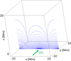 |
Fig. 1. Illustration of the potential arcade which is invariant along the y axis. The arrow depicts the LOS used during the forward modelling (see Sect. 3). This figure is modified from Howson et al. (2020). |
Howson et al. (2020) implement random footpoint motions on the base of the domain (assumed to be representative of photospheric motions). More specifically, the driver is composed of the summation of 2D Gaussians (in space and in time) and has the form v = (vx,vy,0) where
 (2)
(2)
For each i, vi, θi, ri and li are the peak amplitude, direction, centre and length scale of the Gaussian components and ti and τi represent the time of peak amplitude and the duration of the individual Gaussian components, respectively. These variables are derived from the following statistical distributions,
 (3)
(3)
where 𝒩(μ,σ2) and 𝒰(u1,u2) are the normal and uniform distributions, respectively. The mean and variance of the normal distribution are μ and σ2, respectively and u1 and u2 denote the lower and upper bounds for the uniform distribution.
Three different driving timescales are analysed in Howson et al. (2020), of which we shall consider the two extremes, namely τμ = 15 s and τμ = 300 s. The shorter and longer timescales are chosen to replicate the AC and DC heating mechanisms, respectively and hence we shall denote them by τAC and τDC, respectively. The spatio-temporal average of the velocities is set to 1.2 km s−1 in both cases by selecting an appropriate value for vμ. Finally, N is chosen to be a function of the timescale τμ to ensure that a similar number of components in the summation are active at any given time.
The boundaries within this model are periodic on the x and y boundaries. The gradients of the variables are set to zero on both z boundaries with the exception of the velocity driver, which is imposed on the lower boundary. Near the top of the domain, a damping layer is implemented to prevent the reflection of upward waves back into the simulation. It is constructed using v := a(z)v, where a decreases linearly from a(18 Mm) = 1 to a(20 Mm) = 0.99.
2.2. Evolution
Before interpreting the synthetic emission data produced by the forward modelling (see Sect. 3), an understanding of the system’s evolution is helpful. More specifically, we analyse the behaviour of the density, temperature and velocity field.
Figure 2 illustrates the temperature (Fig. 2a), density (Fig. 2b) and velocity profiles (Fig. 2c) at t = 1579 s by taking the median temperature and density (as the mean profile is skewed by large temperatures due to the exclusion of thermal conduction) and average vy along the y axis (invariant direction). This instance in time is chosen as it is fairly representative of the features seen during the complete simulation. We show the results of the ideal (first column), resistive (second column) and viscous (third column) simulations. Within all the simulations, these plasma variable profiles reveal the coronal arcade’s magnetic structure. Due to the absence of thermal conduction, the temperature profiles in the resistive regime do not show these structures as clearly as it potentially would have in coronal conditions. With thermal conduction, these structures would be enhanced due to the diffusion of thermal energy along the magnetic field lines. As for the high density structures in the simulated coronal loops, these may not be realistic as gravity is ignored in these simulations. For both the temperature and density profiles of the resistive simulations, the effect of the zero resistivity region is present for z < 1 Mm. Within the velocity profiles, not only do we see arcade structures, but we observe a signature of the drivers. It is evident that the frequent and short-lived nature of the τAC driver (lower panels of Fig. 2c) generates more distinct small-scale spatial features than in the τDC simulations (upper panels).
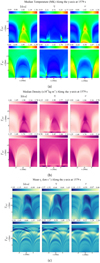 |
Fig. 2. Median temperature (a), density (b), and average vy (c) along the y axis at 1579 s in the ideal (Col. 1), resistive (Col. 2), and viscous (Col. 3) simulations using the τDC (row 1) and τAC (row 2) boundary drivers. |
Howson et al. (2020) found that greater plasma heating occurs when the longer timescale driver was implemented (τDC) in the resistive regime where magnetic energy can be released. The DC-like velocity perturbations are associated with a larger Poynting flux (on average) compared to the τAC driver. In Fig. 2a, in the resistive regime (second column), larger temperatures are present. As optically thin radiation, thermal conduction and mass exchange with the lower atmospheric layers are not modelled here, a large increase in the temperature is observed.
The largest magnetic field perturbations are found near the base of the coronal domain and, as a result, large currents tend to form here. In addition, we also see that large gradients in the magnetic field develop near the separatrix surfaces at x = ±5 Mm. As the magnetic connectivity changes across these planes, footpoint motions on neighbouring field lines can generate strong currents and ultimately, Ohmic heating (Howson et al. 2020). This is apparent in the second column of Fig. 2a, where temperature enhancements are present at the base of the separatrix surfaces. In addition to this Ohmic heating, the dissipation of energy via viscous effects also causes heating. Howson et al. (2020) found that the largest velocity gradients form between the coronal arcades. This was measured using the vorticity of the velocity field. Due to the short timescale driver in the τAC simulation, higher frequency velocity perturbations are present which subsequently generate shorter wave lengths and hence, larger velocity gradients. This results in more viscous heating within the viscous τAC simulation. This viscous heating results in the higher temperature plasma observed on the separatrix surfaces (x ≈ ±5) in the bottom right panel of Fig. 2a.
Howson et al. (2020) found that the kinetic energy is significantly less than the perturbed magnetic energy during all the simulations; hence, the dissipation of kinetic energy within the viscous simulations is expected to have less of an impact than the magnetic energy that is dissipated within the resistive regime. Therefore, Ohmic heating is expected to dominate the plasma heating over the viscous heating (for similar fluid and magnetic Reynolds numbers). Indeed, within Fig. 2a, the heating observed in the resistive simulation (second column) contains hotter plasma than that in the viscous simulation (third column).
3. Forward modelling
3.1. Emission lines and LOS
To forward model the numerical simulations the FoMo code is used (Van Doorsselaere et al. 2016). This code generates optically thin EUV and UV emission lines using the CHIANTI atomic database (Dere et al. 1997; Landi et al. 2013).
For the duration of the simulation, the median temperature of the plasma ranges from approximately 1 MK to 1.5 MK. Nonetheless, the mean temperature can vary from approximately 1 MK to 10 MK. This is due to a small number of locations within the domain of the τDC resistive simulation in which the temperatures are unrealistically high. Approximately 5% of the plasma in this τDC simulation is greater than 6.31 MK (i.e., approximately the maximum temperature that Fe XVI detects). These localised larger temperatures are partially due to the exclusion of optically thin radiation and thermal conduction from the model. In order to cover the majority of the temperatures present, the Fe IX 171 Å, Fe XII 193 Å, and Fe XVI 335 Å emission lines are used. Their peak formation temperatures are approximately log(T) = 5.92 (∼0.839 MK), log(T) = 6.20 (∼1.57 MK) and log(T) = 6.42 (∼2.65 MK), respectively.
Finally, we chose a line-of-sight (LOS) angle aligned with the invariant direction of the initial magnetic field (i.e., the y axis). This is illustrated by the green arrow in Fig. 1.
3.2. Imaging signatures
The (synthetic) total intensity at t = 1579 s in all three emission lines during the ideal, resistive and viscous simulations with the (a) τDC and (b) τAC drivers, is illustrated in Fig. 3. As expected, given the temperature and density profiles (see Fig. 2), the magnetic structure of the coronal arcade is apparent within the total intensity, with the exception of the τAC simulations in Fe XVI (see below). The visible structure for z < 1 Mm in the resistive simulations, caused by the zero resistivity region, is also observable in the total intensity. In general, Fe IX detects the cooler plasma while Fe XII observes the hotter plasma. This hotter plasma is typically found within the central dense arcade in the τDC simulations and along the longer loops bound by the separatrix surfaces in the τAC simulations, in the locations of highest vorticity.
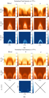 |
Fig. 3. Normalised synthetic total intensity at 1579 s in Fe IX (row 1), Fe XII (row 2), and Fe XVI (row 3) for the ideal (Col. 1), resistive (Col. 2), and viscous (Col. 3) regimes using the (a) τDC and (b) τAC boundary drivers. Every panel is normalised by the spatio-temporal maximum of all simulations in each emission line. The bottom left and right panels in (b) are neglected as very little is detected in the Fe XVI line. |
In this study, the τDC simulation generates hotter plasma than the τAC simulation. Indeed, when comparing the two driving mechanisms, the slow timescale driving generates greater maximum synthetic emission in the plane-of-the-sky (POS) than the AC-like driver for the Fe XII line.
As with the Fe XII synthetic emission, the Fe XVI emission line detects the hotter plasma found within the central arcade in the τDC simulation and in regions of low lying magnetic field line in the τAC simulation. However, due to the reduced heating present in the τAC simulation (in comparison to the τDC simulation) the plasma is not hot enough to be detected by the Fe XVI line within the ideal and viscous regimes. Even within the resistive simulation, very little extremely hot plasma is detected at this time.
The arcade structures are also apparent in the running difference of the synthetic total intensity (current time frame minus the previous with a cadence of 7.2 s) as seen in Fig. 4. Again, the only exception to this is the Fe XVI emission in the τAC simulations. Finer scale features are present within the running difference, with the shorter timescale driver (τAC) creating smaller spatial features as the driver is providing higher frequency velocity perturbations to the system than those in the τDC simulations.
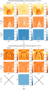 |
Fig. 4. Running difference (cadence of 7.2 s) of the normalised synthetic total intensity at 1579 s in Fe IX (row 1), Fe XII (row 2), and Fe XVI (row 3) for the ideal (Col. 1), resistive (Col. 2), and viscous (Col. 3) simulations using the (a) τDC and (b) τAC boundary drivers. Normalisation and neglected panels are as described in Fig. 3. |
Only within the intensity running difference of the resistive τDC simulation is a structure seen rising between the left and central arcades (see the top two panel of the second column in Fig. 4a where the top of the structure has reached z ≈ 15 Mm). This is the result of adiabatic expansion cause by large temperatures from at the base, between the two arcades, as a result of Ohmic heating. This feature may not be present if thermal conduction was included in the model as it would decrease the large field-aligned temperatures present in our current simulation.
3.3. Doppler velocities
The smaller spatial scale features observed during the total intensity running difference of the τAC simulations are also present within the Doppler velocity signatures. The Doppler velocities are calculated by fitting a (single) Gaussian to the specific intensity and measuring the shift of the Gaussian’s peak from the rest wavelength of the emission line. Figure 5 illustrates the Doppler velocity at 1579 s in the (a) τDC and (b) τAC simulations, where the rows represent the different emission lines and the columns denote the ideal and non-ideal regimes. At this time, there is a dominant blue shift throughout the POS within the τDC simulation. This low variability in the Doppler velocity is due to the long timescale velocity perturbations. Similarly, at other times a dominating red shift is present and the Doppler shift average to zero over the duration of the simulation. Conversely, the τAC driver produces altering red-blue Doppler shifts with smaller spatial features. The arcade’s structure is also observable within both simulation, although it is clearer in the τAC simulation. During the simulations, the general structure and spatial features observed in the Doppler velocity profiles do not change significantly. The magnitude and direction of the Doppler shifts do indeed change but do not alter the analysis provided within this article.
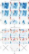 |
Fig. 5. Doppler velocity at 1579 s in Fe IX (row 1), Fe XII (row 2), and Fe XVI (row 3) for the ideal (Col. 1), resistive (Col. 2), and viscous (Col. 3) simulations using the (a) τDC and (b) τAC boundary drivers. |
It is somewhat apparent from the Doppler velocity profiles that higher frequencies features are present when shorter timescale footpoint motions are present (i.e., the τAC simulations compared to τDC simulations). This is confirmed through Fig. 6, which illustrates the Fe XII Doppler velocity as a function of time along five different slits across the POS for the ideal (a) τDC and (b) τAC simulations. The location of these slits in relation to the arcade are indicated in the top left panel. From this point onwards, any analysis shall only be applied to the ideal regime in Fe XII (unless stated otherwise) as there is no significant difference between that and the other emission lines and non-ideal simulations.
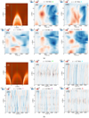 |
Fig. 6. Doppler velocity for Fe XII along various slits as a function of time in the ideal (a) τDC and (b) τAC simulations in km s−1 in panels II–VI. The slits are colour coded in the synthetic total intensity figure in panel I. |
In both Figs. 6a and 6b, propagating features are observed travelling from lower to higher altitudes along the two vertical slits (see panels II:through the apex of the arcade and III:between the arcade structures). To examine these four panels in more detail Fig. 7 was constructed, which restricts the time axis for the four mentioned panels. The solid lines starting on the bottom z boundary at approximately 800 s illustrate how a disturbance travelling at the local Alfvén speed would appear. In particular, we assumed that the lower boundary was perturbed by a linear transverse wave at this time and calculated when it would reach different heights along the slit. These two solid lines (green: Col. II and black: Col. III) are calculated slightly differently. When observing between the arcades (Col. III), the black line is attained by approximately following one single magnetic field line as the slit and field line will have better alignment compared to the green line which passes through the apex of the arcade (Col. II). The green line is therefore calculated by taking multiple magnetic field lines into account. This means the Alfvén travel time is obtained from multiple footpoints to the position in which those field lines meet the slit. Figure 8a illustrates the signature that we would expect to see along the two slits (blue: between arcades and green: through the apex of the arcade) if a linear transverse wave was generated at 800 s on the bottom boundary. These are the same lines as in Fig. 7 with the black line now blue in Fig. 8a. A pictorial representation of the field lines travelled by the wave is given in Fig. 8b before they reach the slits.
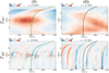 |
Fig. 7. As panels II (through the apex) and III (between arcades) in Fig. 6 for the τDC (top row) and τAC (bottom row) simulations with a truncated time axis between approximately 450 s and 1200 s. The solid lines are the expected signatures of an Alfvén wave excited on the lower boundary at approximately t = 800 s. These are calculated along a single magnetic field line (black: right hand panels) and taking multiple magnetic field lines into account (green: left hand panels). |
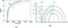 |
Fig. 8. As the lines seen in Fig. 7 now illustrated in panel a along with (b) an illustration of how they are calculated. The black lines depict the arcades structure. For each height zi, tII, i and tIII, i denote the time it takes from z = 0 to reach that height on slits (II: green dashed line) and (III: blue dashed line), respectively. |
From Fig. 8a, we would expect to see shallower gradients when observations along the slit that crosses through the apex – compared to between the arcades – are made. This is the result of the increased amount of time it takes for Alfvénic waves to travel to higher altitudes due to the longer magnetic field lines that cross the slit through the arcade’s apex. Indeed, the propagating structures seen in Fig. 7 (and the zoomed out panels II and III in Fig. 6) coincide with the shape of the overplotted lines. Finally, below the velocity damping layer (z = 18 Mm) (where no observable motion is present), the velocity of the propagating Alfvénic wave features is seen to decrease with altitude. This is simply due to the decrease in Alfvén speed with increasing height (z) (Howson et al. 2020).We note that the change in gradient with altitude corresponds to the decrease in the magnetic field strength (and hence the local Alfvén speed).
Signatures of the Alfvénic waves are also observed in the running difference of the total intensity; however, they are only detected for the τAC (not the τDC) case. Figure 9 illustrates the evolution of the normalised running difference of the Fe XII total intensity along the slit x = 0 Mm (through the arcade’s apex) in the ideal regime (this corresponds to the green slit in panel I of Fig. 6b and the Doppler velocity time-distance contour in the bottom left hand panel of Fig. 7). The green line in Fig. 9 (same as the green line in the bottom left panel of Fig. 7), represents the signature of an Alfvén wave excited at approximately t = 800 s. It is seen to match the shallower gradient features present in the running difference.
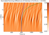 |
Fig. 9. Temporal evolution of the normalised running difference of the Fe XII synthetic total intensity along x = 0 Mm in the ideal τAC simulation. The blue and green lines represent the distance travelled by a fast and Alfvén wave, respectively. |
In Fig. 9, there are also features with larger gradients caused by fast waves. The signature of a fast wave, which is excited at approximately t = 800 s from the base of the domain, is given by the blue line and coincides with the intensity running difference. Similar to the Alfvénic wave, the fast wave slows with increasing altitude due to the decreasing fast speed (Howson et al. 2020). The fast wave is observable in the intensity running difference as it is compressible; however, evidence of the fast wave is not seen in the previous Doppler velocity analysis (see bottom left panel of Fig. 7) as the signature of Alfvénic wave dominates the signal.
As we are able to observe the signatures of the fast and Alfvénic waves, it is possible to estimate the local fast and Alfvén speeds. Using seismology one can estimate, for example, the plasma temperature or the magnetic field strength. However, in our simulation, the uncertainty on the wave speed estimates leads to a wide range of temperature estimates, which does not provide a better constraint on the plasma temperature than the temperature formation range of our emission lines.
Now we shall return to Fig. 6 and consider the lower two horizontal slits, namely panels IV and V. Within the τDC simulation a sharp contrast in the local Doppler velocity is present along x ≈ ±5. This coincides with the location of the separatrix surfaces where larger velocity gradients are predominately found. The reason for the asymmetry of the flows on either side of the separatrix surface is that the magnetic connectivity changes across this plane and thus neighbouring field lines may not be excited in the same way (Howson et al. 2020). This contrast in the Doppler velocity is also present, but less obvious, in the τAC simulations due to the shorter temporal features.
For the τDC simulations (see Fig. 6a), the Doppler velocity in the horizontal slits (see panels IV–VI) shows higher frequency perturbations as well as large spatial structures. To analyse these higher frequencies further, a point in the POS, namely (x, z) = (−9.9.,11.8) Mm, is taken and the behaviour of the Doppler velocity is plotted (black line) in Fig. 10a. The longer period is evidently dominating the signal and originates from the DC boundary driver. To analyse the higher frequency (green line), a smoothed version of the longer period (red line) is subtracted from the original signal. A fast Fourier transform (FFT) (using the standard IDL routine) is then applied to the high frequency signal and shown in Fig. 10b, where the dominant wave periods are annotated within the red boxes. An estimate for the period of the fundamental mode along the initial magnetic field line that passes through the point (x, z) = (−9.9, 11.8) Mm (corresponds to panel VI of Fig. 6a) is obtained by calculating the Alfvén travel time (τA) using
 (4)
(4)
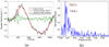 |
Fig. 10. Panel a: Doppler velocity (black) as a function of time at (x, z) = (−9.9, 11.8) Mm, along with a smoothed version of the Doppler velocity curve (red) and the difference between the Doppler velocity and the smoothed Doppler velocity (green). Panel b: corresponding FFT of the high frequency signal (green curve in panel a). |
where ds is an infinitesimal length along the magnetic field line and vA is the local Alfvén speed. The initial conditions are used for this calculation. The period of the fundamental mode is found to be 116 s. This is approximately equal to the period of the high frequency Doppler velocity signal seen in Fig. 10; hence it is reasonable to assume that the high frequency Doppler velocity signal is due to the excitation of standing Alfvénic waves.
The behaviour of the lower, more dominant Doppler velocity frequencies, which are the results of the boundary driver, can also be investigated by implementing an FFT. Figure 11 shows the power of the frequencies observed along the five slits (panels II–VI) across the POS (panel I) for the (a) τDC and (b) τAC simulations. As expected, the long timescale footpoint motions (τDC) produce low frequency velocity perturbations throughout the domain compared to the short timescale driving (τAC). This is seen by the smaller frequency range given for the τDC simulation in comparison to the τAC simulation (see Figs. 11a and 11b, respectively). These smaller and larger frequencies, as well as the structure of the FFTs in Fig. 11, are explained by the FFT of the vy component of the velocity driver averaged along the LOS for each driver (see Fig. 12).
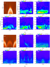 |
Fig. 11. FFT of the Doppler velocity for Fe XII along various slits in the ideal (a) τDC and (b) τAC simulations in panels II–VI. The slits are colour coded in the synthetic total intensity figure in panel I. |
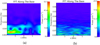 |
Fig. 12. FFT on the bottom z boundary of the LOS average vy of the drivers (a) τDC and (b) τAC. The range in the frequency axis changes between each panel. |
There are some structural features present in the FFT contours of the τAC simulation (see Fig. 11b). Firstly, we shall examine the two vertical slits (panels II and III). When the slit is positioned between two arcades (panel III), it is approximately parallel to the field. As a result the frequencies are similar along the slit. In comparison, when the slit is positioned through the apex of the arcade (panel II), the slit passes through a multitude of magnetic field lines, all of varying length. From the FFT it is clear that the frequencies decrease with increasing altitude. This is because longer magnetic field lines (higher altitudes) have lower natural Alfvén frequencies. This relation is also apparent in the triangular features seen through the horizontal slits in panels V and VI.
Another way to investigate the FFT results is to select a frequency and then analyse the power of this frequency in the POS. Figure 13 shows the power in the POS, with increasing frequencies through panels II to VI, from an FFT analysis for the (a) τDC and (b) τAC simulations. As the τDC driver generates lower frequencies than the τAC driver, different frequencies are used in Figs. 13a and 13b, respectively. Within the τDC simulation, there is no clear correlation between the frequencies and their locations. However, it is evident that with increasing frequency the power decreases as the frequencies are greater than those present in the τDC simulation. Previously, it was shown in Fig. 11b that with increasing altitude (i.e., increasing loop length) the frequencies present in the FFT would decrease. This is indeed the case here for the τAC simulation (see Fig. 13b). With increasing frequency (panels II through VI), the regions of higher power, which approximately outline with arcade’s magnetic field lines, decrease to lower altitudes.
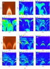 |
Fig. 13. Power from the FFT of the Fe XII Doppler velocity at increasing frequencies through panels II–VI in the ideal (a) τDC and (b) τAC simulations. For reference, panel I illustrates the synthetic total intensity in Fe XII. |
Our final method of analysing the FFT results produces identical conclusions from the previous FFT analysis. Figure 14 shows the frequency with the maximum power of the FFT in the POS for the (a) τDC and (b) τAC simulations. The logarithm of the frequency is taken to help illustrate the features. The τDC simulation does not show any discernible features whereas the short timescale driving (i.e., τAC simulation) generates Doppler velocities whose frequency decreases with increasing altitude (i.e., loop length).
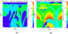 |
Fig. 14. Logarithm of the frequency with the maximum power of the Fe XII Doppler velocity FFT in the ideal (a) τDC and (b) τAC simulations. |
3.4. Line widths
We now investigate the line width of the specific intensity. Figure 15 shows the evolution of the spatial average line width ( ) calculated using the full-width-half-maximum (FWHM) of the Gaussian fitted to the specific intensity (see Gaussian fitting discussion at the start of Sect. 3.3). Panels a–c represent the ideal, resistive and viscous simulations for both the τDC (dashed line) and τAC (solid line) drivers. We show results for the Fe IX (green) and Fe XII (blue) emission lines. Due to the limited differences between the ideal and viscous simulations, the average line widths are very similar (compare panels a and c). On the other hand, the resistive regime produces line widths of approximately 1−3 km s−1 larger than those in the ideal and viscous simulations. The largest increase is observed in the resistive τDC simulation as a result of the substantial heating. Indeed, this is confirmed by the increase in the spatially averaged estimated thermal line width (
 ) shown in Fig. 16. Firstly, to estimate the thermal line width, the mean temperature along the LOS (T̅) was calculated, excluding points from the calculation with temperatures outside the formation range of the ion (Fe IX: ∼0.501–1.33 MK and Fe XII: ∼1.15–2.14 MK). Then, the estimated thermal line width (vth) is calculated and then spatially averaged (
 ). The mean temperature and estimated thermal line width are given by
 (5)
(5)
 (6)
(6)
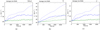 |
Fig. 15. Average line width (FWHM), |

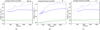 |
Fig. 16. Average estimated thermal line width ( |


respectively. The indices of the coordinates (x, y, z, t) are given by i, j, k and l and ny denotes the number of points along our LOS (i.e., the y axis). The constants, kB, mp and μλ0 denote the Boltzmann constant, the mass of a proton and the atomic weight in proton masses of the emitting element, respectively. The multiplicative constant  seen in the estimated thermal line width (Fig. 16) is to allow for a comparison between the thermal line width and the total line width (Fig. 15). This arises due to the relation between the line width (FWHM) and thermal velocity of a single emission line seen in Eq. (5) of Van Doorsselaere et al. (2016) (it should be noted that there is a minor typo: there is an extra
  in their first expression for λw). In some instances the estimated thermal line width in Fig. 16 is larger than the total line width, which is obviously unphysical. This is due to overestimating the temperature at times within our thermal line width estimation.
3.5. Kinetic energy
In this section, we use the Doppler velocities, previously analysed in Sect. 3.3, to estimate the kinetic energy, and then compare it to the true kinetic energy in the numerical system. The evolution of the kinetic energies (actual and estimated) using the τDC and τAC characteristic timescales are shown in Figs. 17 and 18, respectively. The volume integrated LOS kinetic energy and the estimated kinetic energy, using the spectroscopic data, are calculated using
 (7)
(7)
 (8)
(8)
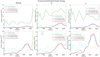 |
Fig. 17. Total (green) and LOS (turquoise) kinetic energy integrated over the full 3D numerical domain compared to the estimated kinetic energy in Fe IX (red), Fe XII (blue) and Fe XVI (orange), during the ideal (Col. 1), resistive (Col. 2) and viscous (Col. 3) τDC simulations. The bottom row is the same as the top row but with a reduced kinetic energy range. |
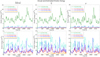 |
Fig. 18. Total (green) and LOS (turquoise) kinetic energy integrated over the full 3D numerical domain compared to the estimated kinetic energy in Fe IX (red), Fe XII (blue) and Fe XVI (orange), during the ideal (Col. 1), resistive (Col. 2) and viscous (Col. 3) τAC simulations. The bottom row is the same as the top row but with a reduced kinetic energy range. |
where vLOS = vy, L is the LOS depth,  is the average density along the LOS, and vD is the Doppler velocity along the LOS (i.e., y axis). Within coronal observations, the LOS depth L and the density profile along the LOS are not easily attainable. The behaviour of the estimated kinetic energy does not change as a result of the length L, which is only a scaling factor (L = 20 Mm). However, to compare the estimated kinetic energy to the actual total kinetic energy, a reasonable estimate of this length is required. As for the density, an average along the LOS can be estimated using line ratios (e.g., Dere et al. 1979; Mason et al. 1979; Landi & Miralles 2014; Polito et al. 2016).
When comparing the kinetic energy in the τDC (Fig. 17) and τAC simulations (Fig. 18), the first stand out feature is there is more variation in the kinetic energy when a short timescale driver is used (Howson et al. 2020). Not only is this seen in the total and LOS kinetic energies but these sharp and frequent gradients are apparent in the estimated kinetic energies too.
Between the ideal and non-ideal simulations, with the same timescale for the boundary driver, the total kinetic energies do not differ significantly, and the LOS kinetic energies only vary slightly. When comparing the different drivers it is found that the τAC simulation is approximately just under one order of magnitude greater than the τDC simulation.
In all the simulations, our chosen LOS (i.e., y axis) generates LOS kinetic energies that underestimate the total kinetic energy. This is to be expected given the multi-directional nature of the velocity driver. As a consequence, even without forward modelling effects, some of the kinetic energy is ‘lost’ along this, and any other, LOS. Obviously, as a result, the estimated kinetic energy underestimates the total kinetic energy. However, it also underestimates the LOS kinetic energy. This is due to both the cancellation of actual velocities along the LOS and only detecting plasma which is within the formation temperature range for the emission line under investigation. A good example of this second case is seen in the Fe XVI estimated kinetic energy. We have shown that Fe IX and Fe XII detect more regions of the domain than Fe XVI does, especially in the τAC simulations. The Doppler velocities at the locations where Fe XVI does not detect the plasma – due to plasma temperatures outwith the formation temperature of Fe XVI – are set to zero; hence a larger underestimation of the LOS kinetic energy is obtained in Fig. 18. Therefore estimates of the total kinetic energy are even more inaccurate. Howson et al. (2020) show that the magnetic energy dominates over the kinetic energy and hence underestimations of the kinetic energy through spectroscopic observations might be insignificant when examining the total energy within the system.
4. Discussion and conclusions
In this paper, we have examined the synthetic emission data produced from simulations of heating in a coronal arcade. We considered resistive, viscous and ideal simulations for velocity drivers with two different characteristic timescales. The drivers were designed to mimic the motions of magnetic footpoints at the base of the corona, with one case akin to AC motions and DC motions in the other. Within our synthetic emission analysis, we used a LOS parallel to the invariant direction of the initial magnetic field (see Fig. 1).
Our model is initially invariant along the y axis, which may not accurately represent the complexity of the corona. As a result, some physical processes (which require a genuinely 3D structure), such as mode coupling and resonant absorption, may be inhibited at the start of the simulations. However, as the simulations progress, perturbations caused by the footpoint driving produce genuinely 3D structures (e.g., see Fig. 5 from Howson et al. 2020), and we do not see any overall change in the relative efficiency of AC and DC drivers once these form. As such, we expect heating to remain larger in the DC cases if a more general field configuration is investigated. Furthermore, even with a genuinely 3D magnetic field structure, the field strength will remain largest at the magnetic footpoints. Therefore, we expect that Ohmic heating will still dominate at low altitudes. Despite these points, a 3D system will have implications for the interpretation of observables. In this article, we take advantage of a specific LOS that is parallel to the (initial) invariant direction. This means the magnetic topology is identifiable in the synthetic emission. Of course, real observations of a less-ordered coronal arcade will be more difficult to analyse.
Within the total intensity, running difference of the total intensity and the Doppler velocity, the arcade’s arch-like structures of the magnetic field are visible regardless of the timescale of the velocity driver. These magnetic field structures are easily identified even though they cannot be measured directly. However, this is not the case when an emission line is chosen that does not fully represent the plasma temperatures present. Indeed, the plasma temperatures within the resistive AC simulation were smaller than the formation temperature range of Fe XVI, and hence only the hotter, low lying magnetic field lines were detected. Cargill (1994) demonstrated, numerically, that plasma exceeding 5 MK is present in loops that have been impulsively heated by nanoflares. The hottest emission line used in this article (Fe XVI) has a peak and maximum formation temperature of approximately 2.65 MK and 6.31 MK, respectively. Therefore, if a hotter emission line is used, such features may be observable. However, in our model we did not include a hotter line as the high temperatures present may be unrealistic due to the absence of thermal conduction and optically thin radiation.
Distinguishing between the associated heating from the AC and DC driving is difficult. The biggest difference we see is the magnitude of the temperature increase (largest for DC driving). However, there is no apparent difference in the spatial distribution of energy release in either case. This translates to the synthetic total intensity, where identifying whether a particular heating event is driven by DC or AC heating may not be possible.
When it comes to comparing Ohmic and viscous heating, resistive simulations do exhibit signatures that are not observed in the viscous cases. For example, in agreement with Van Doorsselaere et al. (2007), the Ohmic heating is found to occur preferentially close to magnetic foot points. Meanwhile, viscous heating is found to occur preferentially at the separatrix surfaces between the coronal arcades (see Howson et al. 2020). However, as there is relatively little energy in the velocity field, the magnitude of this viscous heating is low. As such, we do not see significant differences between the viscous and ideal simulations. As a result, signatures of viscous heating are less visible than those of Ohmic heating and, in these results, are often obscured by changes in the temperature due to adiabatic effects.
As a result of the short-lived velocity perturbations at the magnetic footpoints, short spatial scales are seen in the running difference of the total intensity and the Doppler velocity within the AC simulation. These short timescales in the driver cause higher frequencies than those in the DC simulation. This can be detected via a multitude of methods: analysing the Doppler velocity along a slit as a function of time, taking an FFT along this slit, examining the power of an FFT of Doppler velocity over the POS, and investigating the frequency of the maximum power of a Doppler velocity POS FFT. All of these methods were able to conclude that higher frequencies are present in the AC simulation in comparison to the DC simulation. We were able to identify the signatures of standing Alfvénic waves (see below), despite the random nature of the driver. This resulted in higher frequencies being observed for shorter field lines with higher natural Alfvén frequencies within the τAC simulation.
Propagating features were found when observing the Doppler velocity along vertical slits. These were interpreted as Alfvénic waves and dependent on the position of the slit they appeared to propagate at different rates. A slit that passes through the apex of the arcade, and hence crosses multiple magnetic field lines, produces a slower rate of propagation compared to a slit positioned between two arcades. This is because the distance travelled along the curved magnetic field lines, from the base of the corona to reach a given height on the slit, is farther than the distance travelled along the magnetic field lines that approximately line up with the slit between the arcades. Several different propagating features are identified when observing the running difference of the total intensity along a vertical slit lined up with the apex of the arcade. Some of these features were observed to propagate with the local Alfvén speed and others with the local fast speed. Therefore, within observations, differentiating between Alfvénic and fast waves is attainable as well as identifying the speeds. However, in observations signatures may not be as coherent, especially if the LOS is not directed along the invariant direction of the arcade as in our model.
When observations are taken along horizontal slits, a sharp contrast is seen within the local Doppler velocity at the separatrix surfaces when examining a time-distance plot. These features were more apparent in the DC simulation but still present in the AC simulation. Such a structure occurs due to the magnetic connectivity changing across the separatrix surface and hence neighbouring fieldlines may not be excited in the same way (Howson et al. 2020). This suggests that Doppler shifts are able to identify regions where the connectivity of the coronal field changes.
As well as observing the low frequency Doppler signals during the evolution of the DC simulation, higher frequencies with smaller amplitudes are also present. An estimate of the Alfvén travel time was used to approximate the period of the fundamental mode. This was found to reasonably match the dominant frequencies present in the high frequency signal and hence, suggests that these frequencies are the result of an Alfvénic mode.
The analysis of the line width showed a larger increase within the resistive DC simulation. This is a result of the increased heating present as the magnetic energy is more readily released. Indeed, this increase was confirmed to be a thermal increase as the thermal line width throughout the full 3D domain was estimated and increased more significantly than the other simulations.
An obvious comparison between the estimated kinetic energy (using the spectroscopic data) in the AC and DC simulations was the temporal scales. The AC simulation generated more variation in the kinetic energy as a result of the short timescale velocity driver. When it came to predicting the kinetic energy within the simulations, the LOS caused an underestimation of the kinetic energy. This would be the case for any LOS in this simulation as it is the result of the multi-directional velocity driver, meaning that not all the flows present will line up along a chosen LOS. In the simulations presented here, it is reasonable to assume that there is an equipartition between vx and vy as there is no preferential direction for the horizontal velocity in the driver. Therefore, we should be able to compensate for some of the ‘lost’ kinetic energy. However, this is not necessarily the case in other models or observations. Two further factors that affect the estimation of the kinetic energy are the cancellation of velocity perturbations along the LOS and the plasma temperatures that differ from the formation temperature of the selected emission line. Improvements to the former can be achieved by examining the non-thermal line widths, which can account for the discrepancy between the observed wave energy through Doppler velocities and the true energy in the system (e.g., De Moortel & Pascoe 2012; McIntosh & De Pontieu 2012; Pant et al. 2019). As for the latter, using DEM analysis may minimise the underestimation of the kinetic energy by allowing the most appropriate emission line to be used. Therefore, estimates of kinetic energies within such observations may not capture a significant proportion of the true energy but methods can be used to minimise the error. Howson et al. (2020) showed that the magnetic energy in the simulation dominates the kinetic energy and hence underestimating the kinetic energy does not significantly impact estimates of the total energy within these simulations. However, accurately measuring the observed coronal magnetic field strength and, hence, the associated magnetic field strength is still challenging. Estimates of the kinetic energy are still important in models where the kinetic energy is expected to be comparable to the free magnetic energy, for example in wave models.
In summary, the majority if not all of the observables we have investigated in this paper are relatively easily understood with the knowledge of the evolutionary behaviour of the plasma parameters from the underlying numerical model. However, within observations these parameters are not well known. Our main goal was to establish signatures that could be identified in real observations to distinguish between AC- and DC-like footpoint motions. Firstly, we are able to identify the magnetic structure of the arcade, where the presence of separatrix surfaces is revealed directly by the magnetic field structure but also by contrasts in the local Doppler velocity on either side of the connectivity change. The clearest distinction between the AC and DC models are the frequencies detected through analysis of the Doppler velocities, where, as expected, the DC model exhibits lower frequencies. This is also observed in the spatial scales of the POS Doppler shifts and running difference of the total intensity. Estimating the kinetic energy within the system is challenging because various factors (e.g., multi-directional driver and velocity cancellation along the LOS) prohibit an accurate estimate. Lastly, we note that our model has several limitations (no thermal conduction or optically thin radiation and no coupling to the lower atmosphere) that are likely to affect some of the observational signatures. For example, the extremely large temperatures present in our resistive models will decrease if radiation and thermal conduction are present and this will alter the observables. However, we focused on emission lines with lower temperatures to avoid analysing the unrealistically high temperatures. In addition, we do not expect a large effect on the flows and hence, the analysis of the Doppler velocities presented in this paper.
Acknowledgments
The research leading to these results has received funding from the UK Science and Technology Facilities Council (consolidated grants ST/N000609/1 and ST/S000402/1) and the European Union Horizon 2020 research and innovation programme (grant agreement No. 647214). IDM acknowledges support from the Research Council of Norway through its Centres of Excellence scheme, project number 262622.
References
- Antolin, P., & Van Doorsselaere, T. 2013, A&A, 555, A74 [NASA ADS] [CrossRef] [EDP Sciences] [Google Scholar]
- Arber, T. D., Longbottom, A. W., Gerrard, C. L., & Milne, A. M. 2001, J. Chem. Phys., 171, 151 [Google Scholar]
- Arregui, I. 2015, Philos. Trans. R. Soc. London Ser. A, 373, 20140261 [Google Scholar]
- Cargill, P. J. 1994, ApJ, 422, 381 [Google Scholar]
- De Moortel, I., & Nakariakov, V. M. 2012, Philos. Trans. R. Soc. London Ser. A, 370, 3193 [NASA ADS] [Google Scholar]
- De Moortel, I., & Pascoe, D. J. 2012, ApJ, 746, 31 [Google Scholar]
- De Moortel, I., & Browning, P. 2015, Philos. Trans. R. Soc. London Ser. A, 373, 20140269 [NASA ADS] [Google Scholar]
- Dere, K. P., Mason, H. E., Widing, K. G., & Bhatia, A. K. 1979, ApJS, 40, 341 [NASA ADS] [CrossRef] [Google Scholar]
- Dere, K. P., Landi, E., Mason, H. E., Monsignori Fossi, B. C., & Young, P. R. 1997, A&AS, 125, 149 [NASA ADS] [CrossRef] [EDP Sciences] [Google Scholar]
- Howson, T. A., De Moortel, I., & Fyfe, L. E. 2020, A&A, 643, A85 [NASA ADS] [CrossRef] [EDP Sciences] [Google Scholar]
- Klimchuk, J. A. 2006, Sol. Phys., 234, 41 [Google Scholar]
- Klimchuk, J. A. 2015, Philos. Trans. R. Soc. London Ser. A, 373, 20140256 [NASA ADS] [Google Scholar]
- Klimchuk, J. A., Karpen, J. T., & Antiochos, S. K. 2010, ApJ, 714, 1239 [NASA ADS] [CrossRef] [Google Scholar]
- Landi, E., & Miralles, M. P. 2014, ApJ, 780, L7 [Google Scholar]
- Landi, E., Young, P. R., Dere, K. P., Del Zanna, G., & Mason, H. E. 2013, ApJ, 763, 86 [CrossRef] [Google Scholar]
- Lionello, R., Winebarger, A. R., Mok, Y., Linker, J. A., & Mikić, Z. 2013, ApJ, 773, 134 [NASA ADS] [CrossRef] [Google Scholar]
- Mason, H. E., Bhatia, A. K., Doschek, G. A., & Feldman, U. 1979, A&A, 73, 74 [Google Scholar]
- McIntosh, S. W., & De Pontieu, B. 2012, ApJ, 761, 138 [NASA ADS] [CrossRef] [Google Scholar]
- Pant, V., Magyar, N., Van Doorsselaere, T., & Morton, R. J. 2019, ApJ, 881, 95 [NASA ADS] [CrossRef] [Google Scholar]
- Parnell, C. E., & De Moortel, I. 2012, Philos. Trans. R. Soc. London Ser. A, 370, 3217 [Google Scholar]
- Polito, V., Del Zanna, G., Dudík, J., et al. 2016, A&A, 594, A64 [NASA ADS] [CrossRef] [EDP Sciences] [Google Scholar]
- Van Doorsselaere, T., Andries, J., & Poedts, S. 2007, A&A, 471, 311 [NASA ADS] [CrossRef] [EDP Sciences] [Google Scholar]
- Van Doorsselaere, T., Antolin, P., Yuan, D., Reznikova, V., & Magyar, N. 2016, Front. Astron. Space Sci., 3, 4 [Google Scholar]
- Van Doorsselaere, T., Nakariakov, V. M., Li, B., & Antolin, P. 2020a, Front. Astron. Space Sci., 6, 79 [CrossRef] [Google Scholar]
- Van Doorsselaere, T., Srivastava, A. K., Antolin, P., et al. 2020b, Space Sci. Rev., 216, 140 [Google Scholar]
- Walsh, R. W., & Ireland, J. 2003, A&ARv, 12, 1 [CrossRef] [Google Scholar]
- Winebarger, A. R., Lionello, R., Downs, C., Mikić, Z., & Linker, J. 2018, ApJ, 865, 111 [Google Scholar]
- Yuan, D., & Van Doorsselaere, T. 2016, ApJS, 223, 24 [NASA ADS] [CrossRef] [Google Scholar]
- Yuan, D., Van Doorsselaere, T., Banerjee, D., & Antolin, P. 2015, ApJ, 807, 98 [NASA ADS] [CrossRef] [Google Scholar]
All Figures
|
Fig. 1. Illustration of the potential arcade which is invariant along the y axis. The arrow depicts the LOS used during the forward modelling (see Sect. 3). This figure is modified from Howson et al. (2020). |
| In the text | |
|
Fig. 2. Median temperature (a), density (b), and average vy (c) along the y axis at 1579 s in the ideal (Col. 1), resistive (Col. 2), and viscous (Col. 3) simulations using the τDC (row 1) and τAC (row 2) boundary drivers. |
| In the text | |
|
Fig. 3. Normalised synthetic total intensity at 1579 s in Fe IX (row 1), Fe XII (row 2), and Fe XVI (row 3) for the ideal (Col. 1), resistive (Col. 2), and viscous (Col. 3) regimes using the (a) τDC and (b) τAC boundary drivers. Every panel is normalised by the spatio-temporal maximum of all simulations in each emission line. The bottom left and right panels in (b) are neglected as very little is detected in the Fe XVI line. |
| In the text | |
|
Fig. 4. Running difference (cadence of 7.2 s) of the normalised synthetic total intensity at 1579 s in Fe IX (row 1), Fe XII (row 2), and Fe XVI (row 3) for the ideal (Col. 1), resistive (Col. 2), and viscous (Col. 3) simulations using the (a) τDC and (b) τAC boundary drivers. Normalisation and neglected panels are as described in Fig. 3. |
| In the text | |
|
Fig. 5. Doppler velocity at 1579 s in Fe IX (row 1), Fe XII (row 2), and Fe XVI (row 3) for the ideal (Col. 1), resistive (Col. 2), and viscous (Col. 3) simulations using the (a) τDC and (b) τAC boundary drivers. |
| In the text | |
|
Fig. 6. Doppler velocity for Fe XII along various slits as a function of time in the ideal (a) τDC and (b) τAC simulations in km s−1 in panels II–VI. The slits are colour coded in the synthetic total intensity figure in panel I. |
| In the text | |
|
Fig. 7. As panels II (through the apex) and III (between arcades) in Fig. 6 for the τDC (top row) and τAC (bottom row) simulations with a truncated time axis between approximately 450 s and 1200 s. The solid lines are the expected signatures of an Alfvén wave excited on the lower boundary at approximately t = 800 s. These are calculated along a single magnetic field line (black: right hand panels) and taking multiple magnetic field lines into account (green: left hand panels). |
| In the text | |
|
Fig. 8. As the lines seen in Fig. 7 now illustrated in panel a along with (b) an illustration of how they are calculated. The black lines depict the arcades structure. For each height zi, tII, i and tIII, i denote the time it takes from z = 0 to reach that height on slits (II: green dashed line) and (III: blue dashed line), respectively. |
| In the text | |
|
Fig. 9. Temporal evolution of the normalised running difference of the Fe XII synthetic total intensity along x = 0 Mm in the ideal τAC simulation. The blue and green lines represent the distance travelled by a fast and Alfvén wave, respectively. |
| In the text | |
|
Fig. 10. Panel a: Doppler velocity (black) as a function of time at (x, z) = (−9.9, 11.8) Mm, along with a smoothed version of the Doppler velocity curve (red) and the difference between the Doppler velocity and the smoothed Doppler velocity (green). Panel b: corresponding FFT of the high frequency signal (green curve in panel a). |
| In the text | |
|
Fig. 11. FFT of the Doppler velocity for Fe XII along various slits in the ideal (a) τDC and (b) τAC simulations in panels II–VI. The slits are colour coded in the synthetic total intensity figure in panel I. |
| In the text | |
|
Fig. 12. FFT on the bottom z boundary of the LOS average vy of the drivers (a) τDC and (b) τAC. The range in the frequency axis changes between each panel. |
| In the text | |
|
Fig. 13. Power from the FFT of the Fe XII Doppler velocity at increasing frequencies through panels II–VI in the ideal (a) τDC and (b) τAC simulations. For reference, panel I illustrates the synthetic total intensity in Fe XII. |
| In the text | |
|
Fig. 14. Logarithm of the frequency with the maximum power of the Fe XII Doppler velocity FFT in the ideal (a) τDC and (b) τAC simulations. |
| In the text | |
|
Fig. 15. Average line width (FWHM), |
| In the text | |
|
Fig. 16. Average estimated thermal line width ( |
| In the text | |
|
Fig. 17. Total (green) and LOS (turquoise) kinetic energy integrated over the full 3D numerical domain compared to the estimated kinetic energy in Fe IX (red), Fe XII (blue) and Fe XVI (orange), during the ideal (Col. 1), resistive (Col. 2) and viscous (Col. 3) τDC simulations. The bottom row is the same as the top row but with a reduced kinetic energy range. |
| In the text | |
|
Fig. 18. Total (green) and LOS (turquoise) kinetic energy integrated over the full 3D numerical domain compared to the estimated kinetic energy in Fe IX (red), Fe XII (blue) and Fe XVI (orange), during the ideal (Col. 1), resistive (Col. 2) and viscous (Col. 3) τAC simulations. The bottom row is the same as the top row but with a reduced kinetic energy range. |
| In the text | |
Current usage metrics show cumulative count of Article Views (full-text article views including HTML views, PDF and ePub downloads, according to the available data) and Abstracts Views on Vision4Press platform.
Data correspond to usage on the plateform after 2015. The current usage metrics is available 48-96 hours after online publication and is updated daily on week days.
Initial download of the metrics may take a while.