| Issue |
A&A
Volume 648, April 2021
|
|
|---|---|---|
| Article Number | A125 | |
| Number of page(s) | 21 | |
| Section | Celestial mechanics and astrometry | |
| DOI | https://doi.org/10.1051/0004-6361/202140377 | |
| Published online | 27 April 2021 | |
Characterizing the astrometric instability of extragalactic radio source positions measured with geodetic VLBI
Laboratoire d’astrophysique de Bordeaux, Univ. Bordeaux, CNRS, B18N, Allée Geoffroy Saint-Hilaire,
33615
Pessac,
France
e-mail: cesar.gattano@aiub.unibe.ch; cesar.gattano@obspm.fr; patrick.charlot@u-bordeaux.fr
Received:
18
January
2021
Accepted:
22
February
2021
Context. Geodetic very long baseline interferometry (VLBI) has been used to observe extragalactic radio sources for more than 40 yr. The absolute source positions derived from the VLBI measurements serve as a basis to define the International Celestial Reference Frame (ICRF). Despite being located at cosmological distances, an increasing number of these sources are found to show position instabilities, as revealed by the accumulation of VLBI data over the years.
Aims. We investigate how to characterize the astrometric source position variations, as measured with geodetic VLBI data, in order to determine whether these variations occur along random or preferential directions. The sample of sources used for this purpose is made up of the 215 most observed ICRF sources.
Methods. Based on the geodetic VLBI data set, we derived source coordinate time series to map the apparent trajectory drawn by the successively measured positions of each source in the plane of the sky. We then converted the coordinate time series into a set of vectors and used the direction of these vectors to calculate a probability density function (PDF) for the direction of variation of the source position. For each source, a model that matches the PDF and that comprises the smallest number of Gaussian components possible was further adjusted. The resulting components then identify the preferred directions of variation for the source position.
Results. We found that more than one-half of the sources (56%) in our sample may be characterized by at least one preferred direction. Among these, about three-quarters are characterized by a unique direction, while the remaining sources show multiple preferred directions. The analysis of the distribution of these directions reveals an excess along the declination axis that is attributed to a VLBI network effect. Whether single or multiple, the identified preferred directions are likely due to source-intrinsic physical phenomena.
Key words: astrometry / reference systems / galaxies: nuclei / quasars: general / techniques: interferometric
© C. Gattano and P. Charlot 2021
 Open Access article, published by EDP Sciences, under the terms of the Creative Commons Attribution License (https://creativecommons.org/licenses/by/4.0), which permits unrestricted use, distribution, and reproduction in any medium, provided the original work is properly cited.
1 Introduction
For nearly 30 yr the primary celestial reference system, the International Celestial Reference System (ICRS, Arias et al. 1995), has been extragalactic. It is a kinematic system defined based on fiducial marks representing stable directions in the sky. In practice, this system is realized from a set of celestial objects whose positions on the sky are obtained from observation. The properties of the resulting frame thus depend on the selection of the objects used for this purpose. To tend to the ideal representation, sources with astrometric characteristics that match as closely as possible the above requirements are desired. This has two implications. First, a source should appear point-like at the resolution of the observation technique so that it indeed constitutes a fiducial mark on the sky. Second, its observed position should not vary by more than the level of the measurement noise so that it remains reliable as a fiducial mark over time. This article deals with this second aspect.
Currently, the most accurate realization of the ICRS is the International Celestial Reference Frame (ICRF), which is based on positions of extragalactic radio sources associated with active galactic nuclei (AGN), observed with very long baseline interferometry (VLBI). Since the advent of the VLBI technique and its regular use for geodesy from the late 1970s, three successive realizations of the ICRF have been produced, each of which was in turn formally accepted by the IAU. The first ICRF came into effect in 1998 (Ma et al. 1998), the second, ICRF2, in 2010 (Fey et al. 2015), and the third, ICRF3, in 2019 (Charlot et al. 2020). The last was adopted by the IAU during its XXX General Assembly in August 2018 and is the fundamental celestial reference frame currently in use.
Ever since the first ICRF, the question of the adequacy of certain AGN to serve as fiducial objects was raised due to position variations observed with VLBI. Ma et al. (1998) used the term “arc” sources when a global position (i.e., determined from the entire data set) was not adjusted in the VLBI data reduction process due to significant such variations. More generally, they distinguished 102 sources (denoted “other” sources) out of a total of 608 ICRF sources which showed position instabilities. Gontier et al. (2001) investigated radio source position time series into deeper details for the realization of yearly versions of celestial reference frames in order to assess the stability of the frame axes. Furthermore, Feissel-Vernier (2003) used such time series to define criteria on the basis of which certain sources would be rejected in the selection process of the “defining sources” (i.e., those that define the axes of the frame). Fey et al. (2015) introduced a comparable criterion for the ICRF2 defining source selection process. They also identified 39 “special handling” sources that were treated in the same way as the ICRF arc sources. Charlot et al. (2020) continued along the same line and used coordinate time series as one of the criteria in the selection of the set of defining sources for ICRF3. However, the sources that show significant position instabilities were not categorized separately since they were not found to degrade the frame (in a global sense), and it was then judged preferable to treat all sources in the same way for reasons of consistency of the resulting source positions uncertainties. Alternatively, Karbon et al. (2017) suggested taking care of the source position variations by implementing an automatic algorithm in the VLBI data reduction process.
Categorizing the unstable sources separately or taking care of their astrometric variations is a practical question initially thought to concern a limited number of sources. However, with the data time span becoming longer and the accumulation of the observations, the fraction of sources found to vary has increased. Recently, Gattano et al. (2018) showed that, out of the 647 sources observed in more than 20 geodetic VLBI sessions over the period 1980–2017, the fraction of those that can be considered stable (i.e., with coordinate time series characterized by a white noise process on all time scales) is somewhere between 5% and 40%. In other words, the majority of sources are found to present astrometric variability. Additionally, they noted that stability is even less frequent among the set of the most observed sources, or those monitored on the longest time scales, suggesting that most of the sources would be subject to astrometric variability at the current VLBI accuracy if they had been observed well enough.
While itis a complication for constructing reference frames, the astrometric variability, if intrinsic to the sources, might be of interest for astrophysics. In this study we aim to characterize the position variations for a large number of sources in order to determine whether they occur randomly or along preferred directions, possibly linked to the source physics. Section 2 presents the data set used for this purpose and the method implemented to derive the source position time series. Section 3 presents the algorithm developed to characterize the source position variations and extract information on any favored direction(s) from these variations. The results are given in Sect. 4, first for four individual sources taken as didactic examples throughout this article and then statistically for a sample of 215 sources. Section 5 discusses some elements of the method and proposes an interpretation of our findings.
2 Radio source position time series
2.1 VLBI data set and analysis
The data used for this study consists of dual-frequency (2.3 and 8.4 GHz) VLBI measurements (group delays) acquired on 5099 sources during 6579 VLBI sessions carried out by the International VLBI Service for geodesy and astrometry (Nothnagel et al. 2017) between August 1979 and August 2018. The analysis of these data was accomplished by employing astronomical and geophysical modeling according to the prescriptions of the International Earth Rotation and Reference Systems Service (IERS; Petit et al. 2010). The configuration of the analysis followed standard geodetic practice, though with a specific strategy to derive time series of source positions. A summary of the main features of the modeling and analysis configuration is given below, while the specificity of the analysis for the source positions is presented in Sect. 2.2.
In the analysis process the group delays at the two frequency bands were linearly combined to annihilate the ionospheric effect in the signal propagation. Observations made under 5° of elevation were ignored. Source coordinates, station coordinates and velocities, Earth orientation parameters and their rates, troposphere-related parameters, clock-related parameters, and telescope axis offsets were adjusted during the data reduction process. These parameters were estimated either per session (or on finer timescales) or globally, that is, from the entire data set. The station coordinates and velocities were adjusted globally, apart from discontinuities due to earthquakes. Seismic effects were included for stations that underwent such events. These effects are characterized by a position offset at the moment of the earthquake followed by a nonlinear term modeling the ground relaxation. No-net rotation and no-net translation constraints with respect to ITRF 2014 (Altamimi et al. 2016) were applied to the positions and velocities of a specific set of 41 stations with good observing history. Corrections for the tridimensional displacements of the stations due to oceanic and atmospheric loading were taken into account using the FES2004 model (Lyard et al. 2006) and data from the Atmospheric Pressure Loading Service (APLO; Petrov & Boy 2004). Antenna thermal deformations according to Nothnagel (2009) were also taken into account. Earth orientation parameters and rates were estimated once per session. The nutation offsets were adjusted with respect to the IAU 2006/2000A model which combines the MHB2000 nutation model (Mathews et al. 2002) and the P03 precession quantity (Capitaine et al. 2003). A priori dry zenith delays were derived from local pressure values. Wet zenith delays were estimated every 20 min, while north and east tropospheric gradients were estimated every 6 h. The Vienna Mapping Function (Boehm et al. 2006) was used to map the tropospheric delay to actual elevations. Quadratic clock drift coefficients were estimated every 60 min. Finally, the aberrational effect due to the solar system acceleration around the Galactic center (see, e.g., Kovalevsky 2003; Titov & Lambert 2013; Xu et al. 2013) was corrected in agreement with the modeling for ICRF3 (see Charlot et al. 2020), meaning that a dipolar proper motion field of amplitude 5.8 as yr−1 resulting from an acceleration vector pointing toward the Galactic center was applied to all sources.
2.2 Strategy to derive time series of source positions
Position time series for the entire set of sources present in our observations (i.e., 5099 sources) were derived by running 10 different solutions. The solutions differ from each other in that one-tenth of the sources were treated differently each time. The coordinates for this specific subset of sources were adjusted separately for each session, hence providing time series of positions for the corresponding sources, while the coordinates for the rest of the sources (i.e., nine-tenths of the entire set of sources) were adjusted globally. The 10 subsets were built so that each includes one-tenth of the ICRF3 defining sources (see Charlot et al. 2020). To split the sources into 10 subsets, we first ranked them according to the decreasing number of sessions in which they were observed, after which they were spread across the 10 subsets. The ICRF3 defining sources were treated in the same way but separately from the other sources. Each of 10 subsets is therefore strictly different. In order to obtain consistent orientation for the celestial frame, a no-net rotation condition was applied to the nine-tenths of the ICRF3 defining sources adjusted globally in each of the 10 VLBI global solutions.
From this analysis, we obtained time series of the coordinates α (right ascension) and δ (declination) for each source. In practice the time series are expressed as  and
and  , which represent the offsets with respect to the mean coordinates
  calculated over the entire time series1. We also obtained theassociated uncertainties
  ,
,  and the correlation coefficients between the two coordinates
  for the 5099 sources in our sample. In this denomination, ti is the epoch of the ith session in which the source was observed (i.e., the mean epoch of the observations in the session). In our analysis we assumed that each session-based position is independent, meaning that there is no correlation between the coordinates adjusted from session i with those adjusted from sessionj, i≠ j. For each source, the sessions with too few observations or for which the estimated positions are outliers were discarded. A source is considered to be poorly observed in a session if its position is derived from fewer than three VLBI group delays. A position estimate is considered an outlier if the right ascension or declination is offset from its local mean (calculated on a 2-yr window centered on the assessed data) by six times its local standard deviation (calculated on the same window).
Figure 1 shows the distribution of the sources according to the number of sessions in which they were observed, not counting the sessions that were discarded. Out of the 5099 sources in our data set, 711 were observed in at least 10 valid sessions, 306 in at least 100 sessions, and 72 in at least 1000 sessions. As our interest is to characterize the source astrometric variability, we focused on the sources that have a long observation history. The sample for this study was obtained by selecting the 215 sources for which positions from at least 200 sessions are available.
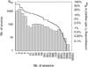 |
Fig. 1 Distribution (in logarithmic scale) of the 5099 sources considered in this analysis according to the number of sessions in which they were observed. Outliers and sessions that had too few observations were discarded (see text). The lower and upper numbers encompassing each bin in abscissa indicate the range of sessions in which the sources comprised in this bin were observed. For example, the sources in the bin
|

2.3 Reduction of the source position time series
In order to reduce the noise level, and hence better assess the potential astrometric variability, the individual measurements were first averaged over some specific periods of time. This was accomplished by splitting the coordinate time series into successive windows of variable lengths including 50 to 100 measurements. The window lengths are set by starting from an initial window of 32 yr (or 64 yr for the sources observed since the 1980s and still observed today), which is first split into two halves, each of which is again split into two halves, and so on until the number of position measurements drops below 100 in every window. In the end, if some windows comprise fewer than 50 measurements the upper boundary of these windows is slightly shifted forward to include a minimum of 50 measurements; if this is not possible the corresponding windows are ignored. Figure 2 shows an example of the time windows derived in this way for a typical source observed over 15 yr.
For each source the reduced coordinate time series  ,
,  were then calculated as the weighted mean of the individual measurements over each window. Here, the set of
  refers to the new time sampling after reduction, whereas the set of ti given above refers to the original time sampling, in other words that resulting from the distribution of the sessions in which thesource was observed. For this calculation the weight of the individual measurements was taken as proportional to
  for the right ascension data and to
  for the declination data. The epochs
  related to the averaged positions were calculated as the weighted mean of the individual epochs ti with weightsproportional to
  . The uncertainties
  and
and  for the reduced coordinate time series and their correlation coefficient
  were derivedby propagating the initial errors through the averaging process assuming no correlation between the coordinates estimated at the different epochs ti.
Figure 3 shows examples of such reduced coordinate time series superimposed onto the initial coordinate time series derived from the VLBI data analysis. Four sources are presented: 0014+813, 0059+581, 1739+522, and 1334−127. The source 0014+813 is a didactic example to illustrate the method devised to characterize the source astrometric variability (see Sect. 3). The other three sources were selected as they each reflect a different astrometric behavior (see results in Sect. 4.1 below).
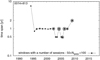 |
Fig. 2 Time windows associated with the reduced positions of the source 0014+813. These windows correspondto the time spans over which session-based coordinates were averaged (see Sect. 2.3). The size of the gray circles is based on the number of sessions within the windows, close to 50 for the smallest circles and near 100 for the largest ones. The abscissa indicates the weighted mean
|

3 Characterization of the source astrometric variability
The method devised to characterize the source astrometric variability aims to determine for each source if there is one (or more) preferred direction(s) on the sky plane along which the source position, as given by the reduced coordinate time series, varies. The method consists of three steps: (1) the reduced coordinate time series are converted into a set of vectors, (2) a probability density function (PDF) is calculated from the direction of those vectors, and (3) the preferred direction is extracted from the PDF.
In the first stage, any two successive positions (from the reduced time series) are converted into a vector with a length  , equal to the angular distance between the two positions, and an angle
  , defined by the direction of the line joining the two positions, counted counterclockwise from the north (i.e., the direction of the declination axis). The errors
  associated with the length and
  associated with the angle of each vector are derived from the combination of the coordinate uncertainties of the two positions and correlation coefficients between right ascension and declination. Figure 4 shows the sets of vectors derived in this way for the four sources investigated.
Based on this set of vectors, a PDF relating to the direction of variation is then calculated. For this purpose, each measurement that characterizes such a direction, meaning each vector, is incorporated into the PDF as a Gaussian function that is parameterized by its center, full width at half maximum (FWHM), and peak value. The center is given by the angle  of the vector, the FWHM is given by
  , and the amplitude is given by the normalized vector length (i.e., the ratio
  of the vector length to its uncertainty). These Gaussian components are then summed and the derived sum is normalized (i.e., it is divided by the sum of the normalized vector lengths) to ensure that the obtained PDF satisfies the property of an integral value equal to one. The PDF is computed modulo 180°, which means that we do not distinguish between opposite directions. In Fig. 4 the PDF for the four sources of interest are materialized as the upper edge of the shaded areas in the insets. We can see that depending on the source the PDF is more or less irregular. The integration of the PDF over only a certain range of angles indicates the probability that the astrometric position of the source varies in that range of directions.
The final step aims to extract the preferred direction of variation of the astrometric position and its uncertainty from the derived PDF. In this determination we leave open the possibility that the astrometric variations occur in multiple directions and adjust in turn from one to five Gaussian components to the computed PDF by using least-squares fits of the form
 (1)
(1)
In this equation, the angle Θn, its standard deviation  , and the amplitude kn of each Gaussian component are the parameters adjusted, with the number of such components, Ncomp, varying between 1 and 5. Initial parameter values are taken from the positions, FWHM, and peak values of the Ncomp highest peaks in the PDF. From this adjustment the preferred directions and their uncertainties are obtained from the Θn and
  values. Additionally, the coefficients kn, which yield the integral of the adjusted Gaussian components, provide a means to estimate the significance of the extracted directions. The closer to one, the more significant the directions. In Fig. 4, the sum of the fitted Gaussian components is superimposed onto the computed PDF and is plotted with a different color for each value of Ncomp (with Ncomp varying from 1 to 5). The sum of the component amplitudes (or integrals) kn indicates the completeness of the model formed by these components with respect to the full PDF. If close to one, the model approaches the PDF. The higher the number of components adjusted, the closer to one the model integral. For our study, the information of interest is the minimum number of components required to approach an integral value of one.
4 Results
4.1 Focus on individual sources
We first present the results obtained for the four sources taken as examples, namely 0014+813, 0059+581, 1739+522, and 1334−127. These results are summarized by the bar charts in Fig. 5. In this figure each gray bar corresponds to a model where a different number of Gaussian components,Ncomp, was adjusted, with Ncomp varying from 1 to 5. The height of these bars is equal to the sum of the integral values of the adjusted components (i.e., the sum of the amplitudes kn in Eq. (1)). For a perfect fit this integral value is equal to 1, whereas in the general case it remains lower than 1. The vertical position of the double-headed arrows plotted within each bar indicates the fraction of this integral associated with the corresponding direction. Table 1 provides the full values for the estimated parameters. It also highlights for each source the model identified as most suitable by the automated treatment described in Sect. 4.2 below.
The source 0014+813 was selected for an evident astrometric position variation in the north–south direction as reflected by the reduced position time series plotted in the right panel of Fig. 3. Considering Ncomp = 1 (red curve in the inset of Fig. 4 and row in bold in Table 1), the derived preferred direction (3 ± 36°) is in line with the expectation from Fig. 3. With a significance of 0.99 (see Table 1) the model also roughly explains the computed PDF. The uncertainty on the estimated direction is large, however, and notably is greater than the 30° limit above which any such uncertainty becomes notmeaningful at the 3σ level. By looking at the details of the source PDF in Fig. 4, we see a secondary peak at about 50°. However, a two-component model does not reveal this secondary peak since the second direction extracted in this case is not significantly different from the first (see the second row for the source 0014+813 in Table 1). Based on our trials, it was foundthat at least three components are needed to extract the information for this secondary peak (see the blue curve in Fig. 4). In this three-component model the first direction extracted, with an uncertainty of 32°, is not reliable, whereas the second and third directions, with respective uncertainties of 14° and 17°, are more constrained. These two directions are at 178° and 54° and match the primary and secondary peaks seen in the PDF. This example shows that examining details of the PDF is necessary to extract the underlying information more completely.
The source 0059+581 appears to be much more complex than 0014+813, as reflected by the position time series in Fig. 3. Its computed PDF, shown in Fig. 4, reveals several peaks of different widths. With a significance of only 0.27, a model with Ncomp = 1 is evidently not sufficient in this case (see Table 1). The model selected by our automatic procedure (bold row in Table 1) is indeed the combination of two components, one that is very well constrained at 107 ± 6°, and another at 19 ± 44° with an uncertainty too large for the direction extracted to be reliable. We note that increasing Ncomp does not significantly change the values and uncertainties of the two components, while it adds new ones, with weaker significance but fine uncertainty, relating to the other peaks seen in the PDF. At Ncomp = 5 the peak of the PDF on the far right side (near ~155°) is still not accounted for by the adjusted model, suggesting that an additional component remains to be identified, which would necessitate pushing the fit further (with Ncomp > 5) to extract it.
The automatic determination of the preferred directions of astrometric variability for the source 1739+522 leads to a three-component model with two well-defined directions at 139 ± 2° and 164 ± 5°, and a third undetermined direction (173 ± 82°), as indicatedby the row printed in bold for this source in Table 1. Interestingly, the first direction seems to be associated with a unique event represented by the sequence of points 14–20 in the reduced position time series in Fig. 3, with point 16 largely offset. In contrast with the source 0059+581 discussed in the preceding paragraph, increasing the number of components to five causes the above undetermined direction to vanish with three strongly determined directions to appear as substitutes. Two of these, at 27 ± 18° and 91 ± 12°, differ significantly from the two directions previously identified when considering the uncertainties (at 2.3σ and 4σ, respectively), while the third direction, at 135 ± 8°, is consistent with the first direction. The source 1739+522 is among the most complex cases encountered in this study, as reflected by the four potential directions of astrometric variations identified.
The fourth source investigated, 1334−127, was selected because it was found to have the highest position stability among the sample of well-observed sources studied by Gattano et al. (2018). In other words, the coordinate time series behavior for this source approaches that of a pure white noise signal when investigated with the Allan standard deviation. For such a source we therefore do not expect to detect any preferred direction of astrometric variation. Looking at Table 1, our automatic scheme returned a single direction with a large uncertainty (131 ± 48°), which confirms the noisy character of the astrometric position variations for this source. This result is also an indicator of stability. Interestingly, the calculated PDF in Fig. 4 reveals two peaks, one of which is not significant while the other one, at 176 ± 6°, seems to be associated only with point 27 in the reduced coordinate time series (Fig. 3). In this respect it should be noted that every reduced point in Fig. 3 is an average over a minimum of 50 VLBI sessions and therefore that point 27 is likely to be a real event that has offset the position of the source over a brief period of time. The presence of a secondary peak in the source PDF shows that such a brief event may be identified and characterized by our method.
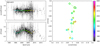 |
Fig. 3 Astrometric variability of the source 0014+813. Left: right ascension and declination time series (upper and lower plot, respectively) represented as offset to the weighted mean coordinates (black dots with error bars plotted in gray) and free from outliers. The colored dots show the associated reduced times series (see Sect. 2.3). The associated colored error bars are smaller than the size of the dots. Right: projection of the reduced coordinate time series on the plane of the sky. The color reflects the weighted mean observing epoch inherent to each reduced position. The numbers enclosed in the colored circles (starting from 0) indicate the successive reduced positions, which allows the apparent source trajectory to be followed on the sky. |
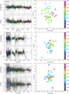 |
Fig. 3 continued. Astrometric variability of the sources 0059+581 (upper plots), 1739+522 (middle plots), and 1334−127 (lower plots). |
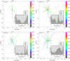 |
Fig. 4 Display of the full sets of vectors characterizing the astrometric position variations for the sources 0014+813, 0059+581, 1739+522, and 1334−127. Each vector connects a pair of successive (reduced) positions in the plane of the sky, as plotted in Fig. 3 for the same four sources. The vector angle is counted from north to east modulo 180°. The color indicates the epoch of the first position in the pair (see the color bar on the right-hand side of each panel). The PDF built from these sets of vectors are given as the upper edge of the shaded areas in the insets. The colored lines in the insetsshow fits to the PDF when one to five components (i.e., the preferred directions) are extracted. |
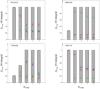 |
Fig. 5 Bar charts showing the results of fitting 1–5 Gaussian components to the PDF of the sources 0014+813, 0059+581, 1739+522, and 1334−127 plotted in Fig. 4. The number of components adjusted is given beneath each gray bar. The height of each bar indicates the total integral value obtained for the corresponding fit. The arrows show the orientation of the resulting preferred directions and the associated uncertainty (represented as a cone around each arrow). The vertical position of the arrows reflects the contribution of the corresponding Gaussian component to the total integral. See Table 1 for the full parameter values. |
Parameters of the preferential directions of astrometric variations identified for the sources 0014+813, 0059+581, 1739+522, and 1334−127.
4.2 Statistics for the entire sample
The study of individual cases, as in the previous section, shows that our algorithm generally identifies one or several directions along which the astrometric variations preferentially occur. Even though individual source inspection maximizes the information extracted from the PDF, it remains desirable to automate the model selection (i.e., determining the number of components, from one to five, that is the most suitable for modeling a given source) so that large samples of sources maybe studied in a consistent way and proper statistics may be derived. We pursued this automation with the goal of characterizing our sample of 215 sources (see Sect. 2.1). For each source, the aim was to automatically select the model with the smallest number of directions (between 1 and 5) that has an integral value approaching 1. In practice, the selection was accomplished by setting a threshold above which the fitted modelwas deemed to be suitable. The number of directions extracted thus depends at some level on the value of the threshold adopted. The higher the threshold, the larger the number of directions. For our study the threshold values considered go from 0.5 to 1. The sources were then categorized according to the number of directions extracted for each value of the threshold in this range. Figure 7 shows the portion of sources in each category (i.e., from one to five directions) as a function of the threshold. From this figure, we see that a majority of sources can be represented by one-direction models up to a threshold value of about 0.95. The rest of the sources are essentially explained by two-direction models. In the following we assume a threshold value of 0.9 to derive further statistics; in other words, models that account for at least 90% of the source PDF are considered. In this case 62% of the sources are found to be characterized by a one-component model, 30% are characterized by a two-component model, and the rest of the sources (8%) need three components or more (see Fig. 7).
Figure 6 shows the distribution of the primary directions (first component in the models) and their uncertainties for the 215 sources in our sample when a threshold value of 0.9 is adopted. In the case of two or more components the distribution of the secondary directions (second component in the models) and tertiary directions, if any, is also plotted. We note that the distribution of the directions (left panel in Fig. 6) is close to homogeneity except for a noticeable excess around 0°, that is, along the declination axis. In other words, all sources considered, it is more likely to find astrometric variations along the declination axis than in any other direction. This peculiarity will be discussed further in Sect. 5.3 below. An issue with these statistics is the reliability of the directions found. In Fig. 6 (right panel) we see that the direction uncertainties are up to 85°. This value makes the corresponding determination basically unreliable since the entire range of directions (from 0 to 180°) falls within the uncertainty range. Assuming a limit of reliability at 3σ, this sets the maximum uncertainty at 30° for a direction to be reliable. This distinction is reflected by two shades of blue in Fig. 6. The histogram in the upper panel of Fig. 8 shows the distribution of the sources according to the number of reliable directions based on this 3σ limit assumption. The colors indicate the number of components included in the original source model. We see from the figure that 44% of the sources are left with no reliable directions when considering the above limit. Conversely, this means that 56% of the sources show at least one well-defined direction along which the astrometric variations preferentially occur. The fraction of sources with only one reliable direction is 34%, with two reliable directions is 17%, and with three reliable directions is 4%. There is also one source that shows four directions and one source that shows five directions.
A final stage in the processing was to check for the presence of duplicates when multiple directions are found. In general, any two directions Θ1 and Θ2 can be considered distinct only if they differ by more than one sigma, that is, if  , where ΔΘ is the shortest difference between Θ1 and Θ2 (i.e., calculated modulo 180°). In all, only six sources were found to have duplicate directions. Removing these duplicate directions thus modifies the previous results only marginally. The adjusted statistics identify 37% of the sources with one preferred reliable direction, 15% with two different preferred reliable directions, 3% with three such directions, and 1% with four directions, a distribution comparable to that in the upper panel of Fig. 8. On the other hand, applying a more stringent criterion, at the three-sigma level, for differentiating the directions (i.e.,
  ) leads to more substantial modifications, as reflected by the histogram in the lower panel of Fig. 8. In this case, 49% of the sources have one preferred reliable direction, 6% have two different preferred reliable directions, and 1% have three such directions. Because the directions extracted generally have limited precision, their combined uncertainty (
 ) is often greater than 30°. As a consequence, the secondary direction is automatically identified as a duplicate and discarded in these cases. In this sense, the 3σ condition is perhaps too strict and the actual distribution may lie between the two distributions shown in the lower and upper panels of Fig. 8.
Complete numerical results for the 215 individual sources studied here are reported in Tables A.1–A.3. These tables list separately the sources showing a unique reliable direction, those with multiple reliable directions, and those where no reliable direction was found.
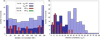 |
Fig. 6 Distribution of the first, second, and third directions extracted from the astrometric variability of the 215 sources in our sample. The directions were derived by assuming a threshold of 0.9 on the model integral (see Fig. 7). The histogram in the left panel shows the primary directions in dark or light blue, the secondary directions in red, and the third directions in green. The histogram in the right panel shows the direction uncertainties with the same color-code. The primary directions are broken into two groups: reliable in dark blue and unreliable in light blue. |
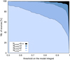 |
Fig. 7 Percentage breakdown of the sources according to the number of components
Ncomp comprised inthe model |

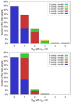 |
Fig. 8 Histogram showing the number of reliable directions for the 215 sources in our sample. The criterion for a reliable direction is to have σΘ < 30°. The color refers to the number of components in the models derived for a threshold of 0.9. Upper panel: histogram before leaving out the duplicate directions. Lower panel: same histogram after leaving out the duplicate directions. The criterion for a direction to be considered a duplicate of a previously identified direction is to present a normalized direction difference smaller than 3 with respect to this other direction (see details in the text). |
5 Discussion
5.1 Consideration about the source sample
Our methodwas applied to reduced coordinate time series with a number of points comprised between 3 and 64. In the minimum case the derived PDF is thus based on only two vectors, or equivalently is the sum of two Gaussian functions. Fitting two Gaussian functions to such a PDF is therefore questionable since it may just return the two initial Gaussians. In Tables A.1 and A.2, we found 10 sources in this situation. Additional sources that have a small number of points are also affected by this limitation, although to a lesser extent. If we reduce the sample to the sources with at least five points, this leaves a subsample of 127 sources. In this subsample, 48% of the sources present at least one preferred direction, while a portion of 17% may show multiple preferred directions, a categorization that is not significantly different from that reported above for the full sample.
In this consideration, it should be remembered that even if the reduced time series consist of a small number of points, the original coordinate time series computed from the VLBI analysis (see Sect. 2.1) consist of at least 200 points, each of which associated with an individual VLBI session. Furthermore, each point in the reduced time series is an average over 50–100 sessions. Consequently, the information contained in these averaged points is robust, and the same is true for the vectors that link them. During the process, the uncertainties are also propagated in order to get meaningful values of these for the extracted directions. These reasons explain why we kept the sources with only a few points in the analysis. It should be noted, however, that the extracted directions for these sources will be subject to more change in the future when additional data points are available.
5.2 Effect of the averaging process
In the description of the averaging process in Sect. 2, we stipulated a condition of having between 50 and 100 sessions within a window to generate one point in the resulting reduced time series. In order to test the impact of this condition, we considered two other possibilities: 25–50 sessions, which extends the sample to sources observed in at least 100 sessions for a total of 305 sources, and 12–25 sessions, which extends the sample to sources observed in at least 50 sessions for a total of 446 sources. Reducing the number of sessions gives access to different timescales for the position variations since the time window over which the individual positions are averaged is also reduced. For example, in the case of source 0014+813, the time scale that is accessed when considering 50–100 sessions is on the order of 0.5–1 yr, whereas it is about 0.25–0.5 yr and 0.1–0.25 yr when considering 25–50 sessions and 12–25 sessions, respectively.
Table 2 compares the results for each of the three ranges of sessions for the sources 0014+813, 0059+581, 1739+522, and 1334−127 taken as examples in this study. The models used for this purpose are those identified in Sect. 4.1. By examining this table, we first note that for the four sources, the shorter the timescale, the stronger (in terms of percentage of the PDF) the unreliable direction extracted (see Col. “Dir. no. 1”). Additionally, the number of reliable directions (see Cols. “Dir. no. 2” and “3”) is found to decrease when the number of sessions considered for averaging is reduced. For the shortest timescales considered (12–25 sessions), it was not possible to get even one direction for the sources 0059+581 and 1334−127 at the end of the process. On the other hand, the uncertainties on the reliable directions when successfully extracted are improved.
The reason of this behavior is that getting to shorter timescales increases the noise level in the reduced coordinate time series. Consequently, any systematics becomes less apparent and thus more difficult to extract. As noted in Sect. 4.2, 62% of the sources are found to be characterized by a one-direction model when considering 50–100 sessions for averaging. This fraction increases to 72% when considering 25–50 sessions for averaging and to 76% when considering only 12–25 sessions. In other words,the number of sources with two or more directions decreases when the averaging time becomes shorter. Additionally, it is also found that the direction extracted at first (i.e., component 1 of the model) is also more often unreliable (i.e., with σΘ > 30°) for shorter timescales.
Examining further the entire sample, we also found that the excess around the declination axis is accentuated when the number of sessions used for averaging decreases. The histogram in the left panel of Fig. 6 shows that there is a bin of 43 sources with the first preferred direction along the declination axis, whereas the rest of the histogram is homogeneous at ~ 20 sources per bin. Hence, 11% (i.e.,  ) of the source sample is in excess. In the case where 25–50 sessions are used for averaging, the bin in excess is found to include 62 sources, with two neighboring bins at 40 sources, while the rest of the distribution is homogeneous at ~ 25 sources per bin. This is equivalent to an excess of
  % of sources with a preferred direction close to the declination axis. If the number of sessions used for averaging to 12–25 is decreased further, the bin in excess becomes even higher, including 78 sources with two neighboring bins at 58 and 70 sources, while the rest of the distribution is homogeneous at approximately 37 sources per bin. The percentage of sources in excess is then
  %. This comparison favors an interpretation of the observed declination excess as an effect inherent to the position time series. The next section discusses this excess in further detail.
Comparison of the models adjusted to the PDF calculated from the position time series of the sources 0014+813, 0059+581, 1739+522, and 1334−127, depending onthe number of sessions used to derive the reduced (i.e., averaged) positions.
5.3 Excess of preferred directions along the declination axis
The sources studied here are associated with AGN. For the most part they are quasars and blazars. According to the unified AGN theory (Antonucci 1993; Urry & Padovani 1995; Padovani et al. 2017), such objects show a pair of symmetric jets that emit in radio, with the forward jet being in the direction of the line of sight for blazars, and slightly tilted from that direction for quasars. At a given observing frequency we only observe the portion of this jet that is not opaque, that is, where the self-absorption optical depth is below unity (Blandford & Königl 1979). The source morphology on VLBI scales then takes the form of a main core plus a potential one-sided jet. Due to opacity effects, the location of the main core may be frequency-dependent (Kovalev et al. 2008).
The existence of such VLBI jets provides specific directions along which astrometric position variations may occur if intrinsic to the sources (i.e., due to the source physics). Under this assumption, VLBI data, as a whole, should not reveal any preferred direction since the AGN jets are not expected to show a preferred orientation in the sky. The distribution of the observed primary directions (i.e., the first direction extracted for each source) should hence be uniform. On the other hand, if the observed astrometric variations relate to systematics in the observing system, such peculiar directions may emerge if the sample of sources considered is large enough.
Our data fall into this second category since we found an excess of primary directions along the declination axis. One known observational aspect is the heterogeneity of the VLBI network coverage with a major difference between the northern and the southern hemisphere. In particular, the limited number of antennas in the south is responsible for the inhomogeneity of the sky coverage of the celestial frame, with the far south being less dense than the northern sky (Fey et al. 2015; Charlot et al. 2020). This also results in right ascension estimates that are more precise than declination estimates in general, due to the lack of north–southbaselines in the network. The error ellipse is then preferably elongated along the direction of declinations, and the vectors extracted are thus more likely to be directed along the declination axis solely due to this asymmetry in the noise. Because of this effect, the interpretation of the directions that are along the declination axis should be treated with caution.
5.4 Astrophysical phenomena possibly involved in the astrometric variability sensed with geodetic VLBI
Our results show that for 56% of the sources in our sample the astrometric position variation occurs in at least one preferred direction. Additionally, multiple preferred directions are found for 7% to 19% of the sources, depending on the criterion used for the identification of duplicate directions (see Sect. 4.2). With the exception of the excess seen along the declination axis, the distribution of the observed directions is uniform, hence leaving open the possibility that these directional astrometric variations come from the source physics. Shabala et al. (2014) brought an argument in this sense since they showed that the radio flux density variability and the astrometric variability are sometimes correlated, with the two being either synchronized or shifted in time. This is also supported by the fact that many sources show extended radio morphology on VLBI scales (e.g., Fey & Charlot 2000). In these cases the observed astrometric position depends on the length and orientation of the VLBI baseline projected onto the sky relative to the source structure and may differ from the VLBI image centroid (Charlot 1990), an effect that can generate astrometric displacements. In the following we review the potential astrophysical phenomena that can induce astrometric position variations. Each of these phenomena is also illustrated in Fig. 9.
The first case (Fig. 9, panel A) is that of radio knots ejected from the VLBI core and moving downstream the jet (e.g., Lister et al. 2009). Simulations of jet evolution enables us to reproduce these phenomena, including the motion of the radio knots (e.g., Hervet et al. 2017), which may be helpful to characterize the corresponding astrometric variability. Due to this evolution, the measured position varies in consequence, and the expected favored direction is that along which the source structure is changing (i.e., the jet direction). Conversely, the astrometric variability may be a good indicator of such structural changes in a source.
In some cases, there is also observational evidence for a bent jet (Fig. 9, panel B), possibly with the presence of VLBI knots moving down this jet. For example, source 3C345 shows these characteristics (Zensus et al. 1995). This makes the extraction of preferred directions from the astrometric variations more complicated (see also Moór et al. 2011) because the measured coordinates vary in a nonlinear way. The jet bending may result from a precession phenomenon2. This is the case for the source 0014+813 (Rozgonyi & Frey 2016), studied in the previous sections, for which a unique direction with an uncertainty of 36°, slightly above the limit of reliability, was found. In the case of a precessing jet, the absolute position of the VLBI core should vary as the jet direction evolves, following an elliptical trajectory on the sky plane. Hypothetically, if the structure is compact enough for the structure effect on the measured source coordinates to be negligible, these measured coordinates should match the absolute position of the VLBI core and thus reproduce its elliptical motion. The observed astrometric variations may therefore be a way to reveal such precessional motion. With our present method the induced effect is expected to manifest itself through a direction that changes with time and is not necessarily aligned with the jet direction. An additional consequence is a degradation of the accuracy of that direction, as extracted with our method, due to not being fixed with time.
Yet another possibility is that the VLBI core itself presents position instabilities due to variations of the jet properties (e.g., during a flare; see Plavin et al. 2019) without showing actual structural changes at the available image resolution. Such fast variations of the properties of the unresolved VLBI core have been found in particular for the TeV-emitting source Mrk 421, where core variability on timescales of weeks was observed (Charlot et al. 2006). In this case, in the event that the radio core moves downstream or upstream, the absolute source position should follow the same path as projected on the sky (Fig. 9, panel C) and the retrieved primary direction should match the projected direction of the jet. Unidirectional astrometric variability without structural changes may then be a way to detect the jitter of the core.
Finally, a scenario is also possible where the sources harbor supermassive binary black hole (SMBBH) systems (or in the more general case supermassive multiple black hole systems). These systems may be formed when galaxies merge, a process that is believed to be an important step in galaxy evolution (Begelman et al. 1980). In this particular case, two different VLBI cores, each associated with one of the black holes, may coexist (Fig. 9, panel D). Such a configuration may be directly identified from VLBI imaging if the two black holes are both radio emitters and are far enough apart, with a separation on the order of a milliarcsecond or more. There is one such case known, 0402+379 (Rodriguez et al. 2006; Bansal et al. 2017). A few other sources are also suspected to harbor similar systems, as indirectly revealed by investigations of the VLBI jet component trajectories in these sources. Such SMBBH candidates include OJ287 (Vicente et al. 1996; Tateyama et al. 1999), 0420−014 (Britzen et al. 2001), 1928+738 (Roos et al. 1993; Roland et al. 2015), 1823+568 (Roland et al. 2013), and 2201+315 (Roland et al. 2020). Regarding the astrometric behavior, it may happen that the source position measured with geodetic VLBI jumps from the location of one black hole to that of the other if the two black holes have similarintensity and vary in time. Since the angular sensitivity of geodetic VLBI is superior to the VLBI image resolution, studies of source position variations may provide further insights into such systems and reveal additional SMBBH candidates, as yet undiscovered. Furthermore, the orbital motion of the two black holes in a binary system may produce jet precession, which would manifest itself as an elliptical trajectory on the sky, as discussed above.
The four scenarios presented in this section are not exclusive. In particular, the first scenario (emergence of radio knots, panel A) is quite common (as evidenced by browsing VLBI image databases such as the Bordeaux VLBI Image Database; Collioud & Charlot 2019) and may coexist with any of the other three scenarios. If occurring in the presence of a SMBBH system (scenario D), the combination of the two phenomena could easily explain the multiple preferred directions that are identified in a number of position time series (see Table A.2). This configuration is discussed by Roland et al. (2020) specifically for source 2201+315, where a scenario with a multiple black hole system is proposed. Looking at our results for this source, we note that up to four preferred directions have been identified. It is interesting that the two predominating ones (at 37 ± 6° and 22 ± 3°; see Table A.2) are consistent with the vector joining the two black holes on the one hand, and with the direction of the radio knot motion as modeled by Roland et al. (2020) on the other hand. Among the other SMBBH systems mentioned above, a single preferred direction has been found for 1823+568. However, some caution is necessary because this determination is based on only two vectors (see Table A.1). For OJ287, our automatic procedure did not return any preferred direction (see Table A.1). Nevertheless, a closer look at our results reveals two reliable directions (located at 137 ± 25° and 73 ± 23°). OJ287 is a BL Lac object and the direction of its VLBI jet is known to oscillate, which was interpreted as being due to a conical helical shape (Vicente et al. 1996). Interestingly, the second direction that we detected is consistent with the sky projection of the helix axis (76°), while its uncertainty is consistent with the pitch angle (20°), both of which were reported by Vicente et al. (1996). For 0420−014 no reliable direction was detected by our automatic procedure, but again a detailed examination of the results shows that the three-component model better fits the source PDF, an indication of a complex behavior. The two other sources listed above, 0402+379 and 1928+738, are not part of the sample studied here. In all, the investigation of these few cases reveals the diversity and richness of the phenomena involved, probably making individual source studies necessary to understand each and every possible case.
 |
Fig. 9 Illustration of four source-intrinsic phenomena that may occur in the inner part of an AGN and induce the astrometric position variations observed with VLBI. The scale used is not realistic. Panel A: ejection and motion of radio knots away from the VLBI core. Panel B: precessing jet. Panel C: VLBI core instabilities. Panel D: dual VLBI core and orbital motion due to the presence of a supermassive binary black hole. |
6 Conclusion and perspective
We developed a method for characterizing VLBI astrometric position variations and for identifying the preferred direction(s) of variability for the radio sources observed with geodetic VLBI. The method consists in calculating a reduced version of the coordinate time series that represent the apparent trajectory of the source’s absolute position drawn on the plane of the sky. These reduced time series are then converted into a set of successive vectors that reflect the direction of variation. From there, a probability density function on the direction of variation is calculated for each source, and a model with a minimum number of Gaussian components is fitted to this function to unveil the underlying preferred directions.
The automation of the procedure facilitates the extraction of the major directions. Additionally, a close scrutiny to the PDF allowed us to obtain a model with a larger number of components in some cases. A preferred direction extracted in such a way is considered to be reliable if its uncertainty is below 30°. Based on the automatically collected results, we found that more than one-half of the sources (56%) among the 215 most observed with geodetic VLBI show at least one such preferred direction. Out of these, about three-quarters are characterized by a unique direction, while the remaining sources show multiple directions. Our results also show that there is an excess of preferred directions along the declination axis. We attribute this excess to a network-related bias coming from the smaller number of north–south baselines in the geodetic VLBI network, thus making declinations generally less precise thanright ascensions. Apart from this excess, the distribution of preferred directions is homogeneous, which indicates that potential source-intrinsic phenomena may be responsible for the observed directions of variations.
The characterization of the source astrometric variability may also bring insights into the source physics. While the astrometric variability may be a good indicator of structural changes within a source, it may also reveal core instabilities in cases where there are no such structural changes. Furthermore, some of the preferred directions detected may evolve with time, which could occur if the VLBI jet is precessing. Finally, the existence of a set of sources with multiple directions brings into question the origin of these directions. They might be a manifestation of as-yet-undiscovered supermassive binary black holes within these objects, a matter of high interest to further understand AGN.
The directions extracted from the astrometric variations, considered solely, do not enable us to go into further details regarding the physical interpretation. A possibility for going forward is to compare those source-dependent directions extracted from astrometric variability with other directions measured independently for the same sources. In this respect we plan to compare ourdetermined directions with the VLBI jet directions as inferred from VLBI images of the sources such as those in the Bordeaux VLBI Image Database (Collioud & Charlot 2019). We also plan to compare these directions with those constructed from the radio-optical position offsets. The Gaia data release 2 (GDR2, Lindegren et al. 2018) comprises more than 550 000 quasars (Gaia Collaboration 2018), of which 265 have been observed in more than 100 geodetic VLBI sessions, hence providing valuable material for comparison. Interestingly, recent studies have showed that radio-optical position offsets tend to align with the VLBI jet direction (Kovalev et al. 2017; Petrov et al. 2019), which points to a relationship between these offsetsand the source physics. Another element suggesting such a relationship comes from the comparisons conducted as part of the ICRF3 work which indicate that sources with extended structures predominate within the subset of ICRF3 sources showing significant radio-optical positional offsets, with a similar predominance also found when examining sources with significant positional offsets between the S/X and K or X/Ka frequency bands (Charlot et al. 2020). All these elements support the presupposed influence of intrinsic source astrophysics in the position determination. Ultimately, these studies, by providing a better understanding of the sources observed in geodetic and astrometric VLBI, should help in further improving the VLBI celestial reference frame, namely the ICRF.
Acknowledgements
This work has been supported by a CNES post-doctoral grant. It relies on geodetic VLBI data and products made available by the International VLBI Service for Geodesy and Astrometry (Nothnagel et al. 2017).
Appendix A Additional material
The tables below provide the estimated preferred directions of astrometric variability for the sample of 215 sources described in Sect. 2.2. These directions were derived from the modeling in Eq. (1), assuming a maximum of five components, and by using the automatic scheme outlined in Sect. 4.2. For each source, the model reported is the model with the smallest number of components that has an integral value of at least 0.9 (see Sect. 3 for more details). The tables list separately the sources with a position variation showing a unique reliable direction (Table A.1), those with a position variation revealing multiple reliable directions (Table A.2), and those where no reliable direction was found (Table A.3).
Preferred directions of VLBI astrometric position variations for the 79 sources of the sample where such variations occur along aunique direction.
Preferred directions of VLBI astrometric position variations for the 41 sources of the sample where such variations occur along two or more directions.
Estimates of the direction of VLBI astrometric position variations for the 95 sources of the sample where such variations occur along no preferred direction.
References
- Altamimi, Z., Rebischung, P., Métivier, L., & Collilieux, X. 2016, J. Geophys. Res. (Solid Earth), 121, 6109 [Google Scholar]
- Antonucci, R. 1993, ARA&A, 31, 473 [Google Scholar]
- Arias, E. F., Charlot, P., Feissel, M., & Lestrade, J.-F. 1995, A&A, 303, 604 [Google Scholar]
- Bansal, K., Taylor, G. B., Peck, A. B., Zavala, R. T., & Romani, R. W. 2017, ApJ, 843, 14 [Google Scholar]
- Begelman, M. C., Blandford, R. D., & Rees, M. J. 1980, Nature, 287, 307 [Google Scholar]
- Blandford, R. D., & Königl, A. 1979, ApJ, 232, 34 [NASA ADS] [CrossRef] [Google Scholar]
- Boehm, J., Werl, B., & Schuh, H. 2006, J. Geophys. Res. (Solid Earth), 111, 2406 [Google Scholar]
- Britzen, S., Roland, J., Laskar, J., et al. 2001, A&A, 374, 784 [Google Scholar]
- Capitaine, N., Wallace, P. T., & Chapront, J. 2003, A&A, 412, 567 [NASA ADS] [CrossRef] [EDP Sciences] [Google Scholar]
- Charlot, P. 1990, AJ, 99, 1309 [NASA ADS] [CrossRef] [Google Scholar]
- Charlot, P., Gabuzda, D. C., Sol, H., Degrange, B., & Piron, F. 2006, A&A, 457, 455 [Google Scholar]
- Charlot, P., Jacobs, C. S., Gordon, D., et al. 2020, A&A, 644, A159 [EDP Sciences] [Google Scholar]
- Collioud, A., & Charlot, P. 2019, in Proceedings of the 24th Meeting of the European VLBI Group for Geodesy and Astrometry [Google Scholar]
- Feissel-Vernier, M. 2003, A&A, 403, 105 [NASA ADS] [CrossRef] [EDP Sciences] [Google Scholar]
- Fey, A. L., & Charlot, P. 2000, ApJS, 128, 17 [Google Scholar]
- Fey, A. L., Gordon, D., Jacobs, C. S., et al. 2015, AJ, 150, 58 [Google Scholar]
- Gaia Collaboration (Mignard, F., et al.) 2018, A&A, 616, A14 [NASA ADS] [CrossRef] [EDP Sciences] [Google Scholar]
- Gattano, C., Lambert, S. B., & Le Bail, K. 2018, A&A, 618, A80 [NASA ADS] [CrossRef] [EDP Sciences] [Google Scholar]
- Gontier, A.-M., Le Bail, K., Feissel, M., & Eubanks, T. M. 2001, A&A, 375, 661 [Google Scholar]
- Hervet, O., Meliani, Z., Zech, A., et al. 2017, A&A, 606, A103 [NASA ADS] [CrossRef] [EDP Sciences] [Google Scholar]
- Karbon, M., Heinkelmann, R., Mora-Diaz, J., et al. 2017, J. Geodesy, 91, 755 [Google Scholar]
- Kovalev, Y. Y., Lobanov, A. P., Pushkarev, A. B., & Zensus, J. A. 2008, A&A, 483, 759 [NASA ADS] [CrossRef] [EDP Sciences] [Google Scholar]
- Kovalev, Y. Y., Petrov, L., & Plavin, A. V. 2017, A&A, 598, A1 [NASA ADS] [CrossRef] [EDP Sciences] [Google Scholar]
- Kovalevsky, J. 2003, A&A, 404, 743 [NASA ADS] [CrossRef] [EDP Sciences] [Google Scholar]
- Lindegren, L., Hernández, J., Bombrun, A., et al. 2018, A&A, 616, A2 [NASA ADS] [CrossRef] [EDP Sciences] [Google Scholar]
- Lister, M. L., Cohen, M. H., Homan, D. C., et al. 2009, AJ, 138, 1874 [Google Scholar]
- Lyard, F., Lefevre, F., Letellier, T., & Francis, O. 2006, Ocean Dyn., 56, 394 [Google Scholar]
- Ma, C., Arias, E. F., Eubanks, T. M., et al. 1998, AJ, 116, 516 [NASA ADS] [CrossRef] [Google Scholar]
- Mathews, P. M., et al. 2002, J. Geophys. Res. (Solid Earth), 107, 2068 [Google Scholar]
- Moór, A., Frey, S., Lambert, S. B., Titov, O. A., & Bakos, J. 2011, AJ, 141, 178 [Google Scholar]
- Nothnagel, A. 2009, J. Geodesy, 83, 787 [Google Scholar]
- Nothnagel, A., Artz, T., Behrend, D., & Malkin, Z. 2017, J. Geodesy, 91, 711 [Google Scholar]
- Padovani, P., Alexander, D. M., Assef, R. J., et al. 2017, A&ARv, 25, 2 [Google Scholar]
- Petit, G., Luzum, B., et al. 2010, IERS Technical Note, 36 [Google Scholar]
- Petrov, L., & Boy, J.-P. 2004, J. Geophys. Res. (Solid Earth), 109, B03405 [Google Scholar]
- Petrov, L., Kovalev, Y. Y., & Plavin, A. V. 2019, MNRAS, 482, 3023 [NASA ADS] [CrossRef] [Google Scholar]
- Plavin, A. V., Kovalev, Y. Y., Pushkarev, A. B., & Lobanov, A. P. 2019, MNRAS, 485, 1822 [NASA ADS] [CrossRef] [Google Scholar]
- Rodriguez, C., Taylor, G. B., Zavala, R. T., et al. 2006, ApJ, 646, 49 [Google Scholar]
- Roland, J., Britzen, S., Caproni, A., et al. 2013, A&A, 557, A85 [Google Scholar]
- Roland, J., Britzen, S., Kun, E., et al. 2015, A&A, 578, A86 [NASA ADS] [CrossRef] [EDP Sciences] [Google Scholar]
- Roland, J., Gattano, C., Lambert, S. B., & Taris, F. 2020, A&A, 634, A101 [Google Scholar]
- Roos, N., Kaastra, J. S., & Hummel, C. A. 1993, ApJ, 409, 130 [Google Scholar]
- Rozgonyi, K., & Frey, S. 2016, Galaxies, 4, 10 [Google Scholar]
- Shabala, S. S., Rogers, J. G., McCallum, J. N., et al. 2014, J. Geodesy, 88, 575 [Google Scholar]
- Tateyama, C. E., Kingham, K. A., Kaufmann, P., et al. 1999, ApJ, 520, 627 [Google Scholar]
- Titov, O., & Lambert, S. 2013, A&A, 559, A95 [NASA ADS] [CrossRef] [EDP Sciences] [Google Scholar]
- Urry, C. M., & Padovani, P. 1995, PASP, 107, 803 [Google Scholar]
- Vicente, L., Charlot, P., & Sol, H. 1996, A&A, 312, 727 [NASA ADS] [Google Scholar]
- Xu, M. H., Wang, G. L., & Zhao, M. 2013, MNRAS, 430, 2633 [Google Scholar]
- Zensus, J. A., Cohen, M. H., & Unwin, S. C. 1995, ApJ, 443, 35 [Google Scholar]

All Tables
Parameters of the preferential directions of astrometric variations identified for the sources 0014+813, 0059+581, 1739+522, and 1334−127.
Comparison of the models adjusted to the PDF calculated from the position time series of the sources 0014+813, 0059+581, 1739+522, and 1334−127, depending onthe number of sessions used to derive the reduced (i.e., averaged) positions.
Preferred directions of VLBI astrometric position variations for the 79 sources of the sample where such variations occur along aunique direction.
Preferred directions of VLBI astrometric position variations for the 41 sources of the sample where such variations occur along two or more directions.
Estimates of the direction of VLBI astrometric position variations for the 95 sources of the sample where such variations occur along no preferred direction.
All Figures
|
Fig. 1 Distribution (in logarithmic scale) of the 5099 sources considered in this analysis according to the number of sessions in which they were observed. Outliers and sessions that had too few observations were discarded (see text). The lower and upper numbers encompassing each bin in abscissa indicate the range of sessions in which the sources comprised in this bin were observed. For example, the sources in the bin
|
| In the text | |
|
Fig. 2 Time windows associated with the reduced positions of the source 0014+813. These windows correspondto the time spans over which session-based coordinates were averaged (see Sect. 2.3). The size of the gray circles is based on the number of sessions within the windows, close to 50 for the smallest circles and near 100 for the largest ones. The abscissa indicates the weighted mean
|
| In the text | |
|
Fig. 3 Astrometric variability of the source 0014+813. Left: right ascension and declination time series (upper and lower plot, respectively) represented as offset to the weighted mean coordinates (black dots with error bars plotted in gray) and free from outliers. The colored dots show the associated reduced times series (see Sect. 2.3). The associated colored error bars are smaller than the size of the dots. Right: projection of the reduced coordinate time series on the plane of the sky. The color reflects the weighted mean observing epoch inherent to each reduced position. The numbers enclosed in the colored circles (starting from 0) indicate the successive reduced positions, which allows the apparent source trajectory to be followed on the sky. |
| In the text | |
|
Fig. 3 continued. Astrometric variability of the sources 0059+581 (upper plots), 1739+522 (middle plots), and 1334−127 (lower plots). |
| In the text | |
|
Fig. 4 Display of the full sets of vectors characterizing the astrometric position variations for the sources 0014+813, 0059+581, 1739+522, and 1334−127. Each vector connects a pair of successive (reduced) positions in the plane of the sky, as plotted in Fig. 3 for the same four sources. The vector angle is counted from north to east modulo 180°. The color indicates the epoch of the first position in the pair (see the color bar on the right-hand side of each panel). The PDF built from these sets of vectors are given as the upper edge of the shaded areas in the insets. The colored lines in the insetsshow fits to the PDF when one to five components (i.e., the preferred directions) are extracted. |
| In the text | |
|
Fig. 5 Bar charts showing the results of fitting 1–5 Gaussian components to the PDF of the sources 0014+813, 0059+581, 1739+522, and 1334−127 plotted in Fig. 4. The number of components adjusted is given beneath each gray bar. The height of each bar indicates the total integral value obtained for the corresponding fit. The arrows show the orientation of the resulting preferred directions and the associated uncertainty (represented as a cone around each arrow). The vertical position of the arrows reflects the contribution of the corresponding Gaussian component to the total integral. See Table 1 for the full parameter values. |
| In the text | |
|
Fig. 6 Distribution of the first, second, and third directions extracted from the astrometric variability of the 215 sources in our sample. The directions were derived by assuming a threshold of 0.9 on the model integral (see Fig. 7). The histogram in the left panel shows the primary directions in dark or light blue, the secondary directions in red, and the third directions in green. The histogram in the right panel shows the direction uncertainties with the same color-code. The primary directions are broken into two groups: reliable in dark blue and unreliable in light blue. |
| In the text | |
|
Fig. 7 Percentage breakdown of the sources according to the number of components
Ncomp comprised inthe model |
| In the text | |
|
Fig. 8 Histogram showing the number of reliable directions for the 215 sources in our sample. The criterion for a reliable direction is to have σΘ < 30°. The color refers to the number of components in the models derived for a threshold of 0.9. Upper panel: histogram before leaving out the duplicate directions. Lower panel: same histogram after leaving out the duplicate directions. The criterion for a direction to be considered a duplicate of a previously identified direction is to present a normalized direction difference smaller than 3 with respect to this other direction (see details in the text). |
| In the text | |
|
Fig. 9 Illustration of four source-intrinsic phenomena that may occur in the inner part of an AGN and induce the astrometric position variations observed with VLBI. The scale used is not realistic. Panel A: ejection and motion of radio knots away from the VLBI core. Panel B: precessing jet. Panel C: VLBI core instabilities. Panel D: dual VLBI core and orbital motion due to the presence of a supermassive binary black hole. |
| In the text | |
Current usage metrics show cumulative count of Article Views (full-text article views including HTML views, PDF and ePub downloads, according to the available data) and Abstracts Views on Vision4Press platform.
Data correspond to usage on the plateform after 2015. The current usage metrics is available 48-96 hours after online publication and is updated daily on week days.
Initial download of the metrics may take a while.