Abundances of neutron-capture elements in thin- and thick-disc stars in the solar neighbourhood

G. Tautvaišienė; C. Viscasillas Vázquez; Š. Mikolaitis; E. Stonkutė; R. Minkevičiūtė; A. Drazdauskas; V. Bagdonas

doi:10.1051/0004-6361/202039979

Home

All issues

Volume 649 (May 2021)

A&A, 649 (2021) A126

Full HTML

Free Access

Issue		A&A Volume 649, May 2021


Article Number		A126
Number of page(s)		20
Section		Galactic structure, stellar clusters and populations
DOI		https://doi.org/10.1051/0004-6361/202039979
Published online		26 May 2021

A&A 649, A126 (2021)

Abundances of neutron-capture elements in thin- and thick-disc stars in the solar neighbourhood^⋆,^⋆⋆

G. Tautvaišienė, C. Viscasillas Vázquez, Š. Mikolaitis, E. Stonkutė, R. Minkevičiūtė, A. Drazdauskas and V. Bagdonas

Astronomical Observatory, Institute of Theoretical Physics and Astronomy, Vilnius University, Saulėtekio Av. 3, 10257 Vilnius, Lithuania
e-mail: grazina.tautvaisiene@tfai.vu.lt

Received: 24 November 2020
Accepted: 5 March 2021

Abstract

Aims. The aim of this work is to determine abundances of neutron-capture elements for thin- and thick-disc F, G, and K stars in several selected sky fields near the north ecliptic pole and to compare the results with the Galactic chemical evolution models, to explore elemental gradients according to stellar ages, mean galactocentric distances, and maximum heights above the Galactic plane.

Methods. The observational data were obtained with the 1.65 m telescope at the Molėtai Astronomical Observatory and a fibre-fed high-resolution spectrograph covering a full visible wavelength range (4000−8500 Å). Elemental abundances were determined using a differential line-by-line spectrum synthesis using the TURBOSPECTRUM code with the MARCS stellar model atmospheres and accounting for the hyperfine-structure effects.

Results. We determined abundances of Sr, Y, Zr, Ba, La, Ce, Pr, Nd, Sm, and Eu for 424 thin- and 82 thick-disc stars. The sample of thick-disc stars shows a clearly visible decrease in [Eu/Mg] with increasing metallicity compared to the thin-disc stars, bringing more evidence of a different chemical evolution in these two Galactic components. Abundance correlation with age slopes for the investigated thin-disc stars are slightly negative for the majority of s-process dominated elements, while r-process dominated elements have positive correlations. Our sample of thin-disc stars with ages spanning from 0.1 to 9 Gyr gives the [Y/Mg] = 0.022 (±0.015)−0.027 (±0.003)⋅age [Gyr] relation. However, for the thick-disc stars, when we also took data from other studies into account, we found that [Y/Mg] cannot serve as an age indicator. The radial abundance-to-iron gradients in the thin disc are negligible for the s-process dominated elements and become positive for the r-process dominated elements. The vertical gradients are negative for the light s-process dominated elements and become positive for the r-process dominated elements. In the thick disc, the radial abundance-to-iron slopes are negligible, and the vertical slopes are predominantly negative.

Key words: Galaxy: evolution / stars: abundances / Galaxy: disk / solar neighborhood

^⋆

Full Table 3 is only available at the CDS via anonymous ftp to cdsarc.u-strasbg.fr (130.79.128.5) or via http://cdsarc.u-strasbg.fr/viz-bin/cat/J/A+A/649/A126

^⋆⋆

Based on observations collected with the 1.65 m telescope and VUES spectrograph at the Molėtai Astronomical Observatory, Institute of Theoretical Physics and Astronomy, Vilnius University, for the SPFOT Survey.

© ESO 2021

1. Introduction

To gain a better understanding of the evolution of the Galaxy and therefore the Universe, it is necessary to know the evolution of the most basic units that comprise it: the chemical elements. The variety of chemical elements found in the spectra of stars is a result of multiple chemical processes and specific conditions. A study of elemental abundances and their distribution in various Galactic components therefore allows us to create Galactic chemical enrichment scenarios and trace back the cosmic events that shaped the current state of the Galaxy.

Most of the observable Universe is formed from hydrogen and helium, which originated during the Big Bang, whereas the remaining elements were formed later in stars (e.g. Coc & Vangioni 2017). Nuclear fusion reactions are responsible for the production of light chemical elements, while elements heavier than A = 56 can only be formed during the capture of free neutrons (Burbidge et al. 1957). Based on timescales of neutron capture versus β⁻-decay ratio, the neutron capture processes are divided into slow (s-process) and rapid (r-process). The s-process takes place at low neutron fluxes (about 10⁵ to 10¹¹ neutrons per cm² per second) when there is enough time for radioactive β⁻ decay to occur before the next neutron is captured. The r-process occurs when the atomic nucleus captures several neutrons due to the high neutron density (about 10²⁴ neutrons per cm³) and high temperature (e.g. Burbidge et al. 1957; Sneden et al. 2008).

The s-processes can occur at various sites and are subdivided into three components: weak, main, and strong (e.g. Kappeler et al. 1989). The weak component prevails in massive stars (> 10 M_⊙) where neutrons are provided by the ²²Ne(α, n)²⁵Mg reaction. This component is partly responsible for the production of the elements from iron to strontium (e.g. Peters 1968; Lamb et al. 1977; Pignatari et al. 2010). Low-mass asymptotic giant branch (AGB) stars are mostly responsible for the main s-process component, which receives free neutrons from the ¹³C(α, n)¹⁶O reaction. This reaction contributes mostly to production of elements beyond A = 90 (e.g. Busso et al. 1999; Käppeler et al. 2011; Bisterzo et al. 2015). The strong s-process component is believed to occur in low-metallicity and low initial mass AGB stars and produces about a half of the solar Pb abundance (e.g. Clayton & Rassbach 1967; Gallino et al. 1998; Travaglio et al. 2001). Estimates of s- and r-process contributions to producing specific elements in various sites vary from study to study (e.g. Arlandini et al. 1999; Travaglio et al. 2004; Sneden et al. 2008; Bisterzo et al. 2014; Shen et al. 2015; Thielemann et al. 2017; Cowan et al. 2021; Haynes & Kobayashi 2019; Mishenina et al. 2019; Siegel et al. 2019, and references therein).

It is known that the r-process is typical in violent conditions with a high density of free neutrons, but environments in which this process takes place are still poorly understood. Several possible sites of the r-process have been proposed: neutrino-induced winds from core-collapse supernovae (Woosley et al. 1994), polar jets from rotating core-collapse supernova (Nishimura et al. 2006), ejecta from neutron star mergers (Freiburghaus et al. 1999) or from neutron star and black hole mergers (Surman et al. 2008). The neutron star merging events were revealed in the LIGO/Virgo experiment by detecting gravitational waves (e.g. Abbott et al. 2017). The neutron star mergers could be a dominant source of r-process dominated elements (Côté et al. 2018), but s-process dominated elements also can be produced, as shown by the recent identification of strontium in the merger of two neutron stars by Watson et al. (2019). The current Galactic chemical evolution (GCE) models also possess uncertainties in accounting for a contribution by the most massive AGB stars (cf. Karakas 2014). Travaglio et al. (2004) have invoked an additional so-called light element primary process (LEPP) in their GCE model in order to solve the deficit of Sr, Y, and Zr as well as the Solar System abundances of s-only isotopes with 90 < A < 130. Recently, the LEPP mechanism was also involved in GCE models by Bisterzo et al. (2017). However, some studies have argued that GCE models could avoid the additional LEPP contribution (cf. Cristallo et al. 2015; Trippella et al. 2016; Prantzos et al. 2018; Kobayashi et al. 2020). The additional source of neutron-capture (n-capture) elements required to explain the solar abundances that led Travaglio et al. (2004) to introduce the additional LEPP process could for instance apparently be explained by the contribution from rotating massive stars (Prantzos et al. 2018). We compared observational results with this new model by Prantzos et al. (2018) and with the semi-empirical model by Pagel & Tautvaisiene (1997), which was the first attempt to model the evolution of n-capture chemical elements in the Galaxy.

Many studies have been dedicated to n-capture element abundance determinations in the Galactic disc field stars (Da Silva et al. 2012; Bensby et al. 2014; Mishenina et al. 2013, 2015, 2019; Nissen 2015, 2016; Nissen et al. 2020, 2017; Zhao et al. 2016; Battistini & Bensby 2016; Spina et al. 2016; Tucci Maia et al. 2016; Delgado Mena et al. 2017, 2019; Luck 2017, 2018a; Reddy & Lambert 2017; Slumstrup et al. 2017; Adibekyan et al. 2018; Guiglion et al. 2018; Magrini et al. 2018; Forsberg et al. 2019; Griffith et al. 2019; Titarenko et al. 2019; Liu et al. 2020, and references therein) with more or fewer chemical elements investigated. The ages of stars, and even less frequently, Galactic radial and vertical locations of stars in the investigated samples are not always determined, however. It is very important to interpret observational results by taking into account as many stellar characteristics as possible. We used an advantage of the new possibilities that were opened by the Gaia space mission (Gaia Collaboration 2016, 2018) in determining accurate stellar locations in the Galaxy and computed slopes of n-capture element abundances in respect to the mean galactocentric distances and distances from the Galactic plane. We would also like to emphasise that the mean galactocentric distances of stars are much more informative than the in situ galactocentric distances that are often used in other studies.

Recently, it was found that abundances of s-process dominated chemical elements are higher in young Galactic open clusters than was predicted by the chemical evolution models. This was raised by D’Orazi et al. (2009), who reported a significant barium overabundance in young open clusters, reaching [Ba/Fe] > 0.6. The enhancement of Ba abundances in young open clusters was confirmed by later studies, but to a lesser degree (see Reddy & Lambert 2017; Spina et al. 2020 for a discussion and possible influence of stellar activity), while abundances of other s-process dominated elements displayed negative or flat abundance trends with increasing age that varied with studies (e.g. Yong et al. 2012; Jacobson & Friel 2013; Mishenina et al. 2013, 2015). The investigations were extended to the Galactic field stars, especially solar twins, even though the accuracy of the age determinations is less precise (e.g. Da Silva et al. 2012; Nissen et al. 2017; Feltzing et al. 2017). Battistini & Bensby (2016) suggested that the trends of abundance ratios [El/Fe] as a function of stellar ages have different slopes before and after 8 Gyr. An increasing trend for solar twins through the entire age range of 10 Gyr was found by Reddy & Lambert (2017) for La, Ce, Nd and Sm, and higher for barium. Spina et al. (2018) also found a strong age-dependent trend for all investigated s-process dominated chemical elements in solar twins. A recent homogeneous study of cluster and field stars in the Gaia-ESO Survey by Magrini et al. (2018), encompassing stars in an age range larger than 10 Gyr, found that an increase in abundances with decreasing object age is more clearly visible for Y, Zr, and Ba, but is less prominent for La and Ce. We compared the n-capture element – age slopes in our sample of stars with those of the solar twins (Spina et al. 2018) and with results by Magrini et al. (2018), as well as with slopes computed for stars investigated by Battistini & Bensby (2016). In order to contribute to solving the so-called barium puzzle, we compared our results with the model by Maiorca et al. (2012), which was computed with the aim to explain the high abundances of s-process dominated elements in young open clusters.

In this study, we extend and complement the results of published studies with a homogeneous abundance analysis of ten neutron capture elements of diverse s/r-process inputs in their production (Sr, Y, Zr, Ba, La, Ce, Nd, Pr, Sm, and Eu) in a sample of 506 FGK dwarfs, subgiants, and giants in the solar neighbourhood. The aim is to investigate how their abundances depend on metallicity, stellar age, the mean galactocentric distance, and the maximum height from the Galactic plane.

The work is structured as follows. In Sect.2 we describe the stellar sample and analysis methods, in Sect. 3 we discuss the elemental abundance trends relative to metallicity and compare with evolutionary models, in Sect. 4 we present the abundance gradients with age and evaluate elemental abundance ratios such as stellar age indicators, while radial and vertical abundance gradients are presented in Sect. 5. We conclude this work with a summary and conclusions in Sect. 6.

2. Stellar sample and analysis

We used archival stellar spectra of the Spectroscopic and Photometric Survey of the Northern Sky (SPFOT) from the Molėtai Astronomical Observatory (MAO, Lithuania) observed by Mikolaitis et al. (2018, 2019) and Tautvaišienė et al. (2020) (hereinafter called Paper I, Paper II, and Paper III). In Paper I and Paper II, all F, G, and K spectral type dwarf and subgiant stars with V < 8 mag were observed within two fields of approximately 20° radii centred at $α (2000) = 161 \overset{°}{.} 03552$ $\alpha(2000) = 161{{\overset{\circ}{.}}}03552$ , $δ (2000) = 86 \overset{°}{.} 60225$ $\delta(2000) = 86{{\overset{\circ}{.}}}60225$ and at $α (2000) = 265 \overset{°}{.} 08003$ $\alpha(2000) = 265{{\overset{\circ}{.}}}08003$ , $δ (2000) = 39 \overset{°}{.} 58370$ $\delta(2000) = 39{{\overset{\circ}{.}}}58370$ , respectively. These fields are preliminary targets of the upcoming ESA PLATO space mission (Rauer et al. 2014; Miglio et al. 2017). In Paper III, all F5 and cooler stars with V < 8 mag were observed within a field of approximately 12° radii centred at α(2000) = 270°, δ(2000) = 66°. This field corresponds to the continuous viewing zone of the NASA TESS space mission (Ricker et al. 2015; Sullivan et al. 2015). Our final list contained 247 stars in the PLATO fields (138 in the first and 109 in the second preliminary field) and 275 in the TESS field. Sixteen stars are in common in the two fields. The list contains no double-line spectroscopic binaries and no stars rotating faster than 25 km s⁻¹. The positions of all programme stars are presented in Fig. 1.

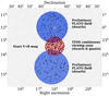Fig. 1.

Positions of all selected programme stars (black dots) observed from the Molėtai Astronomical Observatory in Lithuania. The violet areas denote the preliminary PLATO fields and all observed dwarf stars, while the red area marks the continuous viewing zone of the TESS telescope.

The observations were carried out with the Vilnius University Echelle Spectrograph (VUES; Jurgenson et al. 2014, 2016) mounted on the MAO f/12 1.65 m Ritchey-Chretien telescope. The VUES is a multimode spectrograph with three spectral resolutions (R = 36 000, 51 000, and 68 000) and covers a wavelength range from 4000 to 8800 Å. Stars in Paper I were observed using the R = 68 000 mode, in Paper II we used the R = 36 000 mode, and in Paper III the R = 68 000 mode for the M spectral type stars and the R = 36 000 mode for other objects.

2.1. Stellar atmospheric parameters

The main atmospheric parameters (effective temperature T_eff, surface gravity log g, metallicity [Fe/H], and microturbulence velocity v_t) of the investigated stars were taken from Paper I–Paper III. Figure 2 displays the investigated stars in a surface gravity and effective temperature diagram.

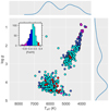Fig. 2.

Investigated stars in a surface gravity and effective temperature diagram showing a density estimation and bivariate distribution.

The stellar atmospheric parameters in these papers were determined from equivalent widths of Fe I and Fe II lines using standard spectroscopic techniques. Effective temperatures were derived by minimising a slope of abundances determined from Fe I lines with different excitation potentials. Surface gravities were found by requiring the Fe I and Fe II lines to give the same iron abundances. The microturbulence velocity values were attributed by requiring the Fe I lines to give the same iron abundances regardless of their equivalent widths. In total, 299 Fe I and Fe II lines were used to compute the stellar atmospheric parameters with the tenth version of the MOOG code (Sneden 1973) and the MARCS grid of stellar atmosphere models (Gustafsson et al. 2008).

2.2. Line list of neutron-capture chemical elements

The line list selection was made based on line quality in terms of their purity and depth, considering only lines that were relatively unblended. The blue region of visible spectra contains many lines of n-capture elements, but this region is disadvantageous because of rather strong blending and lower sensitivity of the CCD detector.

Our main line list was therefore confined to the range 4740 − 6650 Å. An exception was made just for the Sr I line, which is at 4607 Å. This line is relatively clean and deep, and we did not have other good candidates in the redder spectral region. In total, 35 spectral lines were selected (Table 1).

Table 1.

Solar abundances of the investigated chemical elements as determined using two different resolution modes of the VUES spectrograph and values by Asplund et al. (2009).

We used the Gaia-ESO Survey line-list version 5 (Heiter et al. 2021), and took the lines with flags “Yes” or “Undecided”. These labels indicate that the line is “relatively unblended” or “may be useful in some stars”.

Here we also give a summary of the references for transition probabilities (oscillator strengths, log gf), and where applicable, the information for the hyperfine structure and isotopic splitting (hereafter HFS and IS).

The log gf value for the selected line of Sr I was taken from Parkinson (1976), and for all Y II lines we used from Biémont et al. (2011). The values of log gf for all Zr I lines were taken from Biemont et al. (1981), and for the Zr II line, we took the values from Cowley & Corliss (1983). For all Ba II lines the log gf values were taken from Davidson et al. (1992). The strong barium lines have a background line list containing Ba II data and are from Miles & Wiese (1969). The log gf value for the La II 6320.4 Å line was taken from Corliss & Bozman (1962) and the values for the remaining La II lines from Lawler et al. (2001a). We took log gf from the high-quality experimental data by Lawler et al. (2009) for all Ce II lines. Experimental log gf values for two Pr II lines at 5219 and 5322 Å were taken from Li et al. (2007), and for the third line at 5259 Å, no data were provided. We therefore adopted a value from Ivarsson et al. (2001). All Nd II lines were taken from Den Hartog et al. (2003). The oscillator strength experimental value for the Sm II line was taken from Lawler et al. (2006) and from Lawler et al. (2001b) for the Eu II line.

The HFS effects were taken into account to investigate the lines of Ba, La, Nd, Pr, Sm, and Eu. The HFS and IS values were taken for all Ba II lines from Davidson et al. (1992); for the La II 5123, 5303, and 6390 Å lines from Lawler et al. (2001a); for the Nd II 5092 and 5740 Å lines from Den Hartog et al. (2003); for the 5276 Å line from Meggers et al. (1975); for all Pr II lines from Sneden et al. (2009); for the Sm II line from Lawler et al. (2006); and for the Eu II line from Lawler et al. (2001b).

For the remaining lines, for example, La II 4748.7 and 6320.4 Å, the HFS were not provided. These lines are relatively weak, however, and give abundances that are similar to those of the three other La II lines used with HFS. We therefore assume that the HFS effect on our sample stars is small regardless of the spectral resolution.

2.3. Abundance determination

The abundances of all investigated chemical elements were determined using spectral synthesis. To model the synthetic spectra, we used the spectrum synthesis code TURBOSPECTRUM (v12.1.1, Alvarez & Plez 1998). To compute synthetic spectra, we used a set of plane-parallel, one-dimensional, hydrostatic, and constant-flux local thermodynamic equilibrium (LTE) model atmospheres taken from the MARCS¹ stellar model atmosphere and flux library described by Gustafsson et al. (2008). This is the same as assuming that the atmosphere is in statistical equilibrium, homogeneous in abundances, constant in time, R_atm ≪ R_star, and that the energy transport takes place only by radiation and convection. For the barium abundances, we applied the non-local thermodynamic equilibrium (NLTE) corrections taken from Korotin et al. (2015) as the strongest Ba II lines are affected by deviations from LTE. In our sample, for stars with [Fe/H] > 0, the corrections are about −0.027 ± 0.01 dex, in the interval −0.5 < [Fe/H] < 0 the corrections are about −0.033 ± 0.016 dex, and for [Fe/H] < −0.5 the corrections are about −0.06 ± 0.02 dex. In this work, we provide both the LTE and NLTE barium abundances.

The analysis was carried out differentially with respect to the Sun by applying a line-by-line investigation. As our target stars were observed using two different resolutions (36 000 and 68 000), their spectra were investigated differentially to the solar spectra observed in the corresponding resolution mode. In order to increase precision in determining the solar elemental abundances, we averaged the abundances derived from several observations. Table 1 presents the solar abundance values for each investigated line and the corresponding values by Asplund et al. (2009) for comparison. For some stars, due to shallowness of lines, the abundances of some elements were not determined. This was encountered most frequently for the Zr I and Sm II lines.

2.4. Mean galactocentric distances, maximum heights from the Galactic plane, and ages

The mean galactocentric distances (R_mean) and maximum heights from the Galactic plane |z_max| were taken from Paper II and Paper III, where they were computed using input data (parallaxes, proper motions, and coordinates) from the Gaia DR2 catalogue (Luri et al. 2018; Katz et al. 2019; Gaia Collaboration 2016, 2018) and the python-based package for galactic-dynamics calculations galpy by Bovy (2015). Our stellar sample is very well confined in the proximity of the Sun up to 0.14 kpc. We therefore applied a standard distance definition (1/parallax). As recommended, the parallax shift of −0.029 mas from Luri et al. (2018) was adopted, although the effect of this shift on our stellar sample is very small. We did not apply any cut in parallax uncertainties either. We took them into account when we calculated the R_mean and z_max uncertainties. We are aware that for more distant stars in the Gaia DR2, reliable distances should be delivered using a more correct inference procedure that accounts for the nonlinearity of the transformation and the asymmetry of the resulting probability distribution (cf. Bailer-Jones et al. 2018). Our estimates of stellar distances compared with those provided by Bailer-Jones et al. (2018) differ by just 0.0015 ± 0.0048 kpc, which is much smaller than the uncertainties on the distance estimates.

The ages of the investigated stars were taken from Paper I–Paper III, as determined with the UniDAM code by Mints & Hekker (2017). This code combines spectroscopic data with infrared photometry from 2MASS (Skrutskie et al. 2006) and AllWISE (Cutri et al. 2014) and compares them with PARSEC isochrones to derive probability density functions (PDFs) for ages.

The maximum uncertainty allowed for age is 3 Gyr. The mean uncertainty of the age determination as calculated from the uncertainties of individual stars is 2 Gyr, the mean uncertainty of the mean galactocentric distances is 0.2 kpc, and the mean uncertainty of the maximum height from the Galactic plane is 0.05 kpc.

2.5. Evaluation of elemental abundance uncertainties

Systematic and random uncertainties should be taken into consideration. The systematic uncertainties may occur due to uncertainties in atomic data, but they were mostly eliminated because of the differential analysis relative to the Sun.

The random uncertainties may appear because of a local continuum placement and a specific line fitting. A scatter that occurs in averaging abundances from multiple lines of the same element represents the random uncertainty quite well. The average random uncertainties (σ_rand) for every investigated element are presented in Table 2 (the last column). Because we used one Sr I, Zr II, and Eu II line for the abundance determination, we attributed the standard deviation value of 0.07 dex, which was the average of all standard deviations from all the stars and all elements with more than one measured line.

Table 2.

Sensitivity of abundances to the median values of uncertainties in atmospheric parameters and random uncertainties.

Abundance uncertainties may also appear due to uncertainties in atmospheric parameters. The uncertainties in abundances can be measured by calculating the abundance changes that are caused by the error of each individual atmospheric parameter, keeping other parameters fixed. The uncertainties of atmospheric parameters for every star are presented in Paper I–Paper III. The calculated medians of atmospheric parameter determination uncertainties from all stars in our sample are the following: σT_eff = 48 K, σlog g = 0.30, σ[Fe/H] = 0.11, and σv_t = 0.28 km s⁻¹ for dwarfs (log g > 3.5) and σT_eff = 57 K, σlog g = 0.21, σ[Fe/H] = 0.11, and σv_t = 0.22 km s⁻¹ for giants (log g ≤ 3.5). The median dwarf star (log g > 3.5) in our sample has T_eff = 6057 K, log g = 4.20, [Fe/H] = −0.10, and v_t = 1.21 km s⁻¹ and the median giant has (log g ≤ 3.5) T_eff = 4646 K, log g = 2.50, [Fe/H] = −0.14, and v_t = 1.49 km s⁻¹. The sensitivity of the abundances to the median values of uncertainties in atmospheric parameters for stars with log g smaller or larger than 3.5 as well as for solar twins is presented in Table 2. Because most of the investigated chemical elements are ionised, the sensitivity to the uncertainties in log g is highest. The Ba lines, which are relatively strong, are also quite sensitive to v_t.

Finally, the total uncertainty budget was estimated for every elemental abundance determination by taking the uncertainties from stellar parameters as well as random uncertainties into account. We thus calculated σ_El for every given element of every given star as

$\begin{matrix} σ_{El} = \sqrt{σ_{atm}^{2} + {(\frac{σ_{rand}}{\sqrt{N}})}^{2}}, \end{matrix}$ $\begin{aligned} \sigma _{\rm El} = \sqrt{\sigma ^2_{\rm atm}+\left(\frac{\sigma _{\rm rand}}{\sqrt{N}}\right)^2}, \end{aligned}$

where σ_rand is the line-to-line scatter and N is the number of analysed atomic lines. If the number of lines is N = 1, we adopted 0.07 dex for a given element as σ_rand. The uncertainties from four stellar parameters were quadratically summed for every star and gave us σ_atm. The final combined uncertainty σ_El is provided for every element of every star in Table 3.

Table 3.

Atmospheric parameters and abundances of neutron-capture elements.

In Fig. 3 we show a comparison between the expected uncertainties (red line) and the measured dispersion (black line) in metallicity and age bins, where the bin limits are indicated by thin dashed vertical lines. The bin sizes were selected in order to have enough points (at leat five) for the statistical analysis. Because there are fewer the thick-disc stars, the comparison was made for the thin-disc component alone. If the thin disc is well mixed, homogeneous, and well defined, we expect that the scatter of the results in every bin is comparable to the expected uncertainties. In Fig. 4 we show the individual uncertainties (σ_El) as a function of T_eff, log g, and [Fe/H]. Stars of the thin and thick discs (their attribution to the discs is described in the next section) are indicated by different symbols.

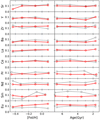Fig. 3.

Observed rms scatter around the median [El/Fe] abundance (grey lines) and expected uncertainties (red lines) in four metallicity and age bins (thin vertical lines). The open circles at every bin are placed at the median value of the [Fe/H] or age of the corresponding bin.

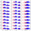Fig. 4.

Uncertainties on the abundance ratios as a function of T_eff, log g, and [Fe/H]. The blue dots represent the thin-disc and the red triangles represent the thick-disc stars. See Sect. 2.5 for details of how the uncertainties have been evaluated.

3. Elemental abundance trends relative to metallicity

We determined the abundances of Sr (453 stars), Y (506 stars), Zr I (307 stars), Zr II (476 stars), Ba (504 stars), La (504 stars), Ce (467 stars), Pr (402 stars), Nd (466 stars), Sm (257 stars), and Eu (488 stars). The results are presented in Table 3 (a full version is available at the CDS). The stars in our sample span an approximate range of T_eff between 3800 and 6900 K, log g between 0.9 and 4.7, [Fe/H] between −1.0 and 0.5 dex, ages between 0.1 and 10 Gyr, R_mean between 5.5 and 11.8 kpc, and |z_max| between 0.03 and 3.73 kpc. These parameters are also presented in Table 3 for convenience. As follows from Paper I–Paper III, there are 424 stars of the Galactic thin disc and 82 of the thick disc in our sample. The [Mg I/Fe I] ratio was adopted to define the thin-disc (α-poor) and thick-disc (α-rich) stars. The last column in Table 3 contains information about which of the Galactic discs a star is attributed to.

We display the elemental abundances versus metallicities² in Fig. 5. For the analysis of the Zr abundances, we used both neutral and ionised lines. The abundance of zirconium was calculated from Zr I lines in 307 stars and from Zr II lines in 476 stars. In the plots, only the [Zr II/Fe I] abundance distribution is depicted, while the [Zr I/H] abundances can be found in Table 3.

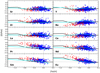Fig. 5.

Elemental abundance trends relative to [Fe I/H]. The blue dots represent the thin-disc stars, and red triangles indicate the thick-disc stars. The continuous lines show the models by Prantzos et al. (2018) (cyan) and Pagel & Tautvaisiene (1997) (black).

Our results coincide well with the previous studies within the uncertainties. Delgado Mena et al. (2017) investigated equivalent widths of Sr, Y, Zr, Ba, Nd, and Eu lines in a large sample of about 1000 FGK dwarfs using spectra of R ∼ 115 000. Mishenina et al. (2013) investigated 276 FGK dwarfs and determined abundances of Y, Zr, Ba, La, Ce, Nd, Sm, and Eu (the abundances of Ba and Eu were determined from spectral synthesis). Forsberg et al. (2019) investigated abundances of Zr, La, and Eu in 196 thin- and 70 thick-disc stars using spectral synthesis. In these studies, the stars were divided into thin- and thick-disc populations, which is essential when GCE models are evaluated, but no ages and kinematic parameters were determined. Bensby et al. (2014) and Battistini & Bensby (2016) analysed the n-capture element abundance and age relations in dwarf stars of the solar neighbourhood (using spectral synthesis, the Y and Ba abundances were determined in the first study, and the Sr, Zr, La, Ce, Nd, Sm, and Eu abundances in the second study). In the study by Magrini et al. (2018), the abundances of Y, Zr, Ba, La, and Ce were homogenised from results obtained with several different methods used in the Gaia-ESO Survey, and their time evolution was investigated.

A remark is due about the strontium abundances. The [Sr/Fe] abundances in the Battistini & Bensby (2016) sample of stars are systematically lower at the solar metallicity by about −0.2 dex. Battistini & Bensby (2016) and Delgado Mena et al. (2017) used the same single neutral line of strontium (4607.33 Å) as we did. Delgado Mena et al. (2017) employed the equivalent width method, while Battistini & Bensby (2016) and we applied spectral synthesis. As the line possibly does not suffer from the HFS splitting (cf. Gratton & Sneden 1994), the method that is used should not play an important role in this case. See Mishenina et al. (2019) for a wider discussion of Sr abundance studies.

Furthermore, we discuss the abundances of n-capture chemical elements divided into groups depending on their origins as well as abundance gradients as a function of stellar age, mean galactocentric radii, and maximum heights from the Galactic plane. We compare the results with model predictions and previous studies if available.

3.1. Sr, Y, and Zr

Sr, Y and, Zr belong to the first s-process peak and are called the light s-process (ls) dominated chemical elements. While the s-process is the key contributor to their abundances, their detailed production is still debated. As displayed in Table 4, studies sometimes provide different contributions of s-process to production of these elements (Arlandini et al. 1999; Sneden et al. 2008; Bisterzo et al. 2014; Prantzos et al. 2020). Moreover, these elements are produced not only by the main but also by the weak s-processes and by the r-process.

Table 4.

Solar percentage of s-process input for the n-capture elements.

According to Bisterzo et al. (2014), in addition to the s-process contributions, there are pure r-process contributions of 12, 8, and 15% to Sr, Y, and Zr, respectively. Hence, the origin of about 8% of Sr and by 18% of Y and Zr is still unclear. As proposed by Travaglio et al. (2004), the missing LEPP process might be present in low-metallicity massive stars. However, this hypothesis was challenged for instance by Cristallo et al. (2015), Trippella et al. (2016), Prantzos et al. (2018), and Kobayashi et al. (2020). In Fig. 5 we compare our observational results to the model by Prantzos et al. (2018). In this grid of models, the authors used metallicity-dependent isotopic yields from low- and intermediate-mass stars and yields from massive stars that include the combined effect of metallicity, mass loss, and rotation for a large grid of stellar masses and for all stages of stellar evolution. The yields of massive stars are weighted by a metallicity-dependent function of the rotational velocities, constrained by observations as to obtain a primary-like ¹⁴N behaviour at low metallicity and to avoid overproduction of s-elements at intermediate metallicities. The semi-empirical model by Pagel & Tautvaisiene (1997), the first attempt to model the evolution of the n-capture elements in the Galaxy, is also displayed to show the advancement of modern models.

As shown in Fig. 5, the [Sr, Y, Zr/Fe] values follow the thin-disc models by Prantzos et al. (2018) and Pagel & Tautvaisiene (1997) quite well. Regarding the abundance values in the thick-disc stars, in our sample of stars they are quite close to those in the thin-disc stars and do not provide strong evidence to support the finding by Delgado Mena et al. (2017) that in metal-deficient thick-disc stars the zirconium abundances are much higher than in the thin-disc stars. A similar pattern to ours was reported in Mishenina et al. (2013). This question should be explored further.

3.2. Ba, La, and Ce

The production for barium, lanthanum, and cerium, the so-called heavy s-process (hs) elements belonging to the second s-process peak, are clearly dominated by the s-process (see Table 4). As indicated in Käppeler et al. (2011), all isotopes beyond A = 90, except for Pb, are mainly produced by the s-process main component. The remaining element yields are produced via the r-process component. Thus, a similar production pattern for all three elements should be reflected in their abundances.

Figure 5 shows that the chemical evolution of Ba, La, and Ce is indeed very similar. In the Prantzos et al. (2018) baseline model, the LIMS contribution to Ba, La, and Ce abundances reaches its maximum at around [Fe/H] = −0.4 and then starts to drop, creating a downward trend at sub-solar metallicities. Figure 5 shows that a convex shape of the model should have its maximum at [Fe/H] of about −0.2 dex, and should start accounting for the LIMS input at higher metallicities (∼ − 0.7 dex), as was modelled by Pagel & Tautvaisiene (1997). This is also very clearly seen in the Ba and Ce abundance trends. The model by Prantzos et al. (2018) reflects elemental abundances in the stars of super-solar metallicities quite well.

The [Ba, La, Ce/Fe] ratios in the thick-disc stars are slightly lower than in the thin-disc sample stars of the neighbouring metallicity. They still agree with the thin-disc model by Pagel & Tautvaisiene (1997), however. They also indicate that the time-delay of the main s-process contribution should be longer in the model by Prantzos et al. (2018).

3.3. Pr and Nd

Praseodymium and neodymium are attributed to the second s-process peak as well. They have a more mixed origin than Ba, La, and Ce, however, because about half of their abundances comes from the s-process main component and the other half from the r-process (see Table 4).

For praseodymium, our results agree well with the Prantzos et al. (2018) model from slightly sub-solar to super-solar metallicities. [Pr/Fe] are more enhanced at metallicities lower than −0.2 dex, however. The lower LIMS effect on Pr compared to Ba, La, or Ce is compensated for by the r-process. The model by Prantzos et al. (2018) therefore has no expressed peak at around −0.4 dex. However, our observational data for Pr indicate that the r-process contribution to the praseodymium production may be higher. The model underestimation of Pr abundances at lower metallicity stars of our sample could indicate that the r-process effect was underestimated both by Prantzos et al. (2018) and Pagel & Tautvaisiene (1997). The trend of [Pr/Fe] versus metallicity is quite similar to the [Sm/Fe] and [Eu/Fe] trends.

The model by Prantzos et al. (2018) fits to the distribution of [Nd/Fe] ideally. Differently from [Pr/Fe], at sub-solar metallicities [Nd/Fe] abundances show flatter behaviour. This corresponds to the high percentage of s-process input in Nd than in Pr.

The thick-disc stars have higher ratios of Pr and Nd to Fe than in the case of more s-process dominated elements, which qualitatively agree well with the GCE predictions for the thin disc. However, in the metal-deficient thick-disc stars, the abundance difference between the s- and r-process dominated chemical elements is stronger.

3.4. Sm and Eu

Samarium and europium are two r-process dominated elements we investigated. About 70% of Sm is made by this process, and more than 90% of Eu. The s-process main component is responsible for the remaining abundances of these elements.

Samarium abundances were determined for fewer stars than in the case of other chemical elements. Nevertheless, the abundances form an increasing trend towards lower metallicities, as expected for the element with a high r-process input. Compared with the Mishenina et al. (2013) sample, some stars have higher [Sm/Fe] ratios. Compared with the sample from Battistini & Bensby (2016), however, the overall patterns of the samarium abundance results agree well. The [Eu/Fe] abundance results for the stars in our sample show a complete agreement with other studies discussed in this work. Recently, Forsberg et al. (2019) debated that europium abundances might be super-solar at the solar metallicity. They investigated abundances of Zr, La, Ce, and Eu in a sample of 291 giants in the Galactic thin and thick discs. Their Fig. 5 shows that the abundances of zirconium, which were determined from the neutral lines, agree with the results of other studies, while the abundances of La, Ce, and Eu, which were determined from the ionised lines, are systematically higher. This may be caused by systematic uncertainties in determining a surface gravity of these stars. The authors used the stellar atmospheric parameters from Jönsson et al. (2017), who reported that the surface gravities are overestimated while comparing the results with the Gaia stellar parameter benchmark values. If this is the case, the abundances of the ionised elements are overestimated as well.

The thin- and thick-disc stars show higher abundances, especially for europium, compared with the s-process dominated elements. This agrees with the GCE theory.

If all the stars in our sample can be correctly attributed to the thin and thick discs, which can hardly be achieved for all studies, the chemical evolution models both by Prantzos et al. (2018) and Pagel & Tautvaisiene (1997), which agree with each other quite well, are slightly too low. Further developments in modelling the r-process yields and time delays in production of these elements are continuing. New production sites are about to be revealed (see e.g. Côté et al. 2019; Schönrich & Weinberg 2019). The additional origin in Eu production could be related to neutron star mergers and other sources, as discussed in the introduction. Matteucci et al. (2014), for instance, found that the models with only neutron star mergers producing Eu or mixed with type II supernovae can reproduce the observed Eu abundances in the Galactic disc. However, Côté et al. (2019) emphasised that the neutron star mergers cannot reproduce the observational constraints at all metallicities on their own. They proposed to consider an input of so-called magnetorotational or other rare types of supernovae acting in the early universe, but fading away with increasing metallicity.

3.5. Comparison of the light and heavy s-process element abundances

The reliability of s-process yields in the GCE models can be verified by comparing the abundances of heavy and light s-process dominated elements. It is common to monitor the s-process efficiency through the relative abundances of the s-elements with neutron magic numbers N = 50 at the Zr peak with respect to those with the neutron magic numbers N = 82 at the Ba peak. These nuclei are mainly synthesised by the s-process and act as bottlenecks for the s-process path because of their low neutron capture cross-sections.

Prantzos et al. (2018) compared in their Fig. 17 the computed [hs/ls] versus [Fe/H] evolution model with observations for the unevolved thin- and thick-disc stars by Delgado Mena et al. (2017). The [hs/ls] ratios were computed using the average abundance ratios of Ba, Ce, and Nd for the [hs/Fe] ratios, while for the [ls/Fe] ratios, the averages of Sr, Y, and Zr were taken. From the comparison, the authors concluded that the yields used in their baseline GCE model are reliable and reproduce observational trends of unevolved stars. However, they did not take into account that measurements of the specific elements considered in the observational average [hs/Fe] and [ls/Fe] abundances were not present for every star due to the quality of the observed spectra. If the authors had taken only the stars from the Delgado Mena et al. (2017) sample with the abundances of all the six chemical elements determined, it would be visible that the agreement is poor. This is also seen when the model is compared with our sample stars (see Fig. 6). As the heavy s-element, we also included lanthanum. The abundances of this chemical element were absent in Delgado Mena et al. (2017). When the plots with and without La are compared, the systematic difference in the [hs/ls] ratios is just 0.003 dex.

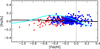Fig. 6.

Ratio of heavy (Ba, La, Ce, Nd) and light (Sr, Y, Zr) s-process dominated element abundances with respect to [Fe I/H] compared with the GCE model predictions by Prantzos et al. (2018) (cyan line) and the thin-disc model by Pagel & Tautvaisiene (1997) (black line). Our results are marked as blue circles for the thin-disc and as red triangles for the thick-disc stars.

The model agreement with the observations appears to have been better if the convex shape of the model had its maximum not at the [Fe/H] of −0.4 dex, but at about −0.2 dex, and would start accounting for the LIMS input at higher metallicities (about −0.7 dex). The GCE model by Prantzos et al. (2018) still has to be further developed by investigating the roles of the yields from rotating massive stars and low- and intermediate-mass stars. This is also visible from the comparisons of the model in the [El/Fe] versus age plots that we discussed in Sect. 2.4.

3.6. Comparison of the s- and r-process dominated element abundances

The abundance patterns of s- and r-process dominated elements allow us to show how different star formation histories are in the Galactic discs. In Fig. 7 we compare abundance ratios of r-process dominated element europium and s-process dominated element barium [Eu/Ba] versus [Fe I/H] with the GCE model predictions for the thin disc by Prantzos et al. (2018) and by Pagel & Tautvaisiene (1997), as well as with a pure r-process ratio derived using the percentages of Bisterzo et al. (2014) and the solar abundances of Grevesse et al. (2007). The GCE models of the thin disc clearly have to be further developed in order to account for the higher europium production and for other r-process dominated chemical elements such as samarium (Fig. 8).

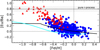Fig. 7.

[Eu/Ba] ratio with respect to [Fe I/H]. Symbols are the same as in Fig. 6. The dotted line and the shadowed area of ±0.1 dex uncertainty represent a pure r-process ratio derived using the percentages of Bisterzo et al. (2014) and the solar abundances of Grevesse et al. (2007).

Fig. 8.

[Sm/Ba] ratio with respect to [Fe I/H]. Symbols are the same as in Fig. 7.

For the evolution of the thick disc, Guiglion et al. (2018) have recently raised the idea that the abundance ratios of [Eu/Ba] might be constant with metallicity. Other r-process dominated elements investigated in their study, gadolinium and dysprosium, showed an abundance to barium ratios that decreased with increasing metallicity. The authors concluded that their observations clearly indicate a different nucleosynthesis history in the thick disc between Eu and Gd-Dy. In our study, we clearly see the decline of [Eu/Ba] ratio as a function of metallicity as in other studies (e.g. Battistini & Bensby 2016; Delgado Mena et al. 2017; Magrini et al. 2018).

The [Eu/Ba] and [Sm/Ba] ratios are close to the pure r-process line for metal-poor thick-disc stars, meaning that the r-process was the only n-capture process active at the beginning of the formation of the thick disc. The difference between samarium-to-barium abundance ratios in the thin and thick discs is not as prominent as in the case of europium. This agrees with the relatively lower production of samarium in the r-process sites.

A comment could also be made about the [Eu/Ba] ratios in the super-solar metallicity stars. Delgado Mena et al. (2017) reported that the [Eu/Mg] ratios in the thin-disc stars start to increase with increasing metallicity. This might be caused by the underestimation of barium abundances using the equivalent width method applied in this study or other methodological reasons. Another study by Trevisan & Barbuy (2014), which was dedicated especially to the analysis of metal-rich stars, shows a quite flat but slightly decreasing trend until [Eu/Ba] of about −0.2 dex at [Fe/H] of about +0.5 dex. In our study, the stars span about [Fe/H] of +0.3 dex and show the same trend as in Trevisan et al. and other studies (e.g. Battistini & Bensby 2016; Magrini et al. 2018).

3.7. [Eu/Mg] ratio

The study of magnesium and europium abundances in different galactic components is essential for determining the formation and evolution of the Galaxy. Mashonkina & Gehren (2001) studied 63 cool stars with metallicities ranging from −2.20 dex to 0.25 dex. In their Fig. 8, the authors pointed to a tendency of [Eu/Mg] ratios to decrease with increasing metallicity both for the thin- and thick-disc stars. They also found an overabundance of Eu relative to Mg in three halo stars. However, in 2003 they reanalysed the sample including 15 additional moderately metal-deficient stars (Mashonkina et al. 2003), and an overabundance of Eu relative to Mg was determined only for two thick-disc and halo stars (see Fig. 5 in their paper). Furthermore, Delgado Mena et al. (2017) also found an almost flat [Eu/Mg] (see their Fig. 15), suggesting that these two elements receive an important contribution from supernovae progenitors of similar masses. However, Guiglion et al. (2018) recently addressed the topic in the AMBRE project for a large sample of FGK Milky Way stars in a range of metallicities very similar to ours. They reported a decreasing [r/α] trend for increasing metallicity, from which one of the main conclusions in their work was derived.

The europium-to-magnesium abundance ratios versus metallicity in our sample of stars are presented in Fig. 9. The magnesium abundances were taken from Paper II and Paper III. We found that the [Eu/Mg] ratio in the investigated metallicity range tends to slightly decrease with increasing metallicity for the thin-disc stars. This is even more evident for the thick-disc stars. The abundances of Eu are higher when they are compared to the semi-empirical model by Pagel & Tautvaisiene (1997), which foresees the production of Eu by type II supernova alone. The model by Prantzos et al. (2018) extends far too high (mainly because of the Mg modelling uncertainties, see their Fig. 13).

Fig. 9.

[Eu/Mg] ratio with respect to [Fe I/H]. Symbols are the same as in Fig. 6.

We have mentioned the negative trend of [r/α] with increasing metallicity for the thin-disc stars found by Guiglion et al. (2018) in the AMBRE project. Based on 25 thick-disc stars in the AMBRE sample, however, it was difficult to make a confident conclusion about the thick disc. Our sample of 76 thick-disc stars shows an even stronger decrease of [Eu/Mg], as well as [r/α], with increasing metallicity than in the thin-disc stars. This indicates a different chemical evolution of these two Galactic components.

4. Abundance gradients with age

Figure 10 shows distributions of element-to-iron ratios as a function of stellar ages. The figure also includes the best linear fits to the [El/Fe I] versus age and theoretical models by Prantzos et al. (2018) and Maiorca et al. (2012).

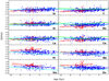Fig. 10.

Elemental-to-iron abundance ratios as a function of age. The blue dots and red triangles represent the thin- and thick-disc stars of our study, respectively. The green lines represent the models by Maiorca et al. (2012) and the cyan lines those by Prantzos et al. (2018). The blue lines are the linear fits for the thin-disc stars of this work and the red lines show the thick-disc stars, with a 95% confidence interval for the ordinary least-squares regressions. The vertical dashed lines indicate the adopted age of the Sun (4.53 Gyr).

The determined best linear fits to the [El/Fe I] and age relations are presented in Table 5. We provide the slopes, y-intercepts, Pearson correlation coefficients (PCC), and standard errors of the linear fits.

Table 5.

Best linear fits to the [El/Fe I]−age distributions in dex Gyr⁻¹ and the Pearson correlation coefficients for the thin disc stars and comparison with other works.

For comparison, we also computed fits using data by Battistini & Bensby (2016) for Sr, Zr, La, Ce, Nd, Sm, and Eu, and data by Bensby et al. (2014) for Y and Ba. We took data of the thin-disc stars (TD/D < 0.5) with age determination uncertainties better than 3 Gyr. The determined slopes from our sample agree well with the slopes determined using the Battistini & Bensby (2016) and Bensby et al. (2014) studies, but there are more stars with higher barium abundances in the sample of Bensby et al. (2014), probably because this study included more stars with larger mean galactocentric distances. In some of these young stars, which are often quite active, the high Ba abundances may be caused by the NLTE effects, which are under-accounted for the Ba II lines that emerge in the upper layers of stellar atmospheres (Reddy & Lambert 2017).

Table 5 also shows slopes obtained for solar twins in the recent study by Spina et al. (2018) and for the Galactic thin-disc stars with ages younger than 8 Gyr computed by Magrini et al. (2018). The authors investigated abundances of Y, Zr. Ba, La, and Ce using internal data of the Gaia-ESO Survey.

In Fig. 11 we compile all [El/Fe I] trends as a function of age determined in our work. With increasing age, all the s-process dominated elements in the thin-disc stars of our sample show negative or flat trends (for [Sr/Fe], [Y/Fe], and [Ba/Fe], the downward trends being most clearly visible), while the r-process dominated elements have slightly positive or flat trends. These patterns agree with the GCE theory, which predicts a noticeable production of s-process dominated elements during the evolution of the Galactic disc.

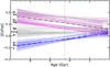Fig. 11.

Compilation of [El/Fe I] trends as a function of age for the thin-disc stars. The continuous purple lines represent the r-process dominated elements Eu, Sm, and Pr. The thick dash-dotted line is an averaged trend of these element-to-iron abundance ratios. The continuous blue lines represent the s-process dominated elements Y, Sr, and Ba. The thick dash-dotted line is an averaged trend of these element-to-iron abundance ratios. The grey continuous lines are for elements with negligible [El/Fe I] age trends (Nd, Ce, La, and Zr). The continuous magenta line represents the [Mg/Fe I] age correlation. The shadowed areas show the 95% confidence interval for the regressions. The vertical dashed line marks the solar age.

In Fig. 10 we also compare the observational data with the models by Prantzos et al. (2018) and Maiorca et al. (2012). The model by Maiorca et al. (2012) closely follows our stars for Zr, but it has a slightly positive offset for Y at older ages. The model by Prantzos et al. (2018) predicts quite flat trends for Sr, Y, and Zr from around 9 Gyr to the youngest objects, with a slightly positive offset for Sr and Y and a negative offset for Zr.

Our [Ba, La, Ce/Fe] ratios are close to the chemical evolution model by Maiorca et al. (2012) for the sub-solar ages. The younger stars display not so high abundance values as are predicted by the model, however. This is expected because the model was oriented to account for the higher abundances of Ba, La, and Ce that are observed in open clusters. The authors suggested that the observed enhancements might be produced by nucleosynthesis in AGB stars of low mass (M < 1.5 M_⊙) if they release neutrons from the ¹³C(α, n)¹⁶O reaction in reservoirs larger by a factor of four than assumed in more massive AGB stars. In the current literature, the same assumptions on the formation of the ¹³C neutron source for all stars between 1 and 3 M_⊙ are reported. However, these elements are not so abundant in the field stars, and Marsakov et al. (2016), for example, discussed on the basis of 90 open clusters the reasons for the s-process dominated element overabundances in open clusters, which include high and elongated orbits, for instance.

The model by Prantzos et al. (2018) predicts a completely different behaviour for Ba, La, and Ce than the model by Maiorca et al. (2012). The model reaches its abundance peak at around 8 Gyr and then slightly decreases with decreasing age. Compared to our results, the model overestimates the abundances in the older stars and slightly underestimates the abundances in the youngest stars.

As the [Ba/Fe] abundances in our work are very close to those of [La/Fe] and [Ce/Fe] and show close to solar abundances at young ages, we can state that our study does not support the barium puzzle anomaly (also opposed by Reddy & Lambert 2017) and does not require the additional intermediate process (i-process), as proposed by Cowan & Rose (1977), Mishenina et al. (2015). Stars with ages younger than 2 Gyr in our sample are dwarfs and unevolved giants. The mean uncertainty in their age determination is (+1.17; −0.62) Gyr.

Praseodymium, neodymium, samarium, and europium have a significant input from r-process in their production. As r-process requires quite harsh conditions to occur, a production peak of such elements took place at earlier times in the Galaxy. For these elements the Prantzos et al. (2018) model predicts a steady decline in [El/Fe] ratios with decreasing ages, but still steeper than our results suggest, especially for europium.

The 76 thick-disc stars of our sample show uncertain [El/Fe I] trends with age (Fig. 12). Of the r-process dominated elements, only Sm shows a slightly positive trend. Its accuracy is quite low, however. In contrast, of the s-process dominated elements, only Y has a more noticeable but also quite uncertain trend. The [Mg/Fe I] versus age slope is also presented for comparison. We address the question of age dependence of the elemental abundance rations in the following section.

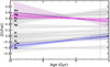Fig. 12.

Compilation of [El/FeI] trends as a function of age for the thick-disc stars. The continuous purple line represents the r-process dominated element Sm, which alone shows a slight trend, but with a quite low accuracy. The continuous blue line represents the s-process dominated element Y, which has a more noticeable trend than the others. The grey continuous lines are for elements with negligible trends of [El/FeI] vs. age. The continuous magenta line represents the [Mg/FeI] age correlation. The shadowed areas show the 95% confidence interval for the regressions. The vertical dashed line marks the solar age.

4.1. [Y/Mg] as an age indicator for the thin-disc stars

As was proven previously, [Y/Mg] is a sensitive age indicator for solar twins (Da Silva et al. 2012; Nissen 2015, 2016; Spina et al. 2016; Tucci Maia et al. 2016). Feltzing et al. (2017) showed that this relation depends on [Fe/H] and flattens for stars with lower than solar metallicities. They concluded that the [Y/Mg] versus age relation is unique to solar analogues. However, Slumstrup et al. (2017) confirmed that the empirical relation between [Y/Mg] and age as presented by Nissen (2016) also holds for the solar metallicity helium-core-burning giants. Nissen et al. (2017) also confirmed that the abundances of the Kepler LEGACY stars, with asteroseismic ages, support the same relation between [Y/Mg] and stellar age as was previously found for solar twins. The sub-sample of Kepler LEGACY stars in Nissen et al. (2017) has a metallicity range similar to that of solar twins (−0.15 < [Fe/H] < +0.15), but the range of effective temperatures is much wider (5700 < T_eff < 6400 K).

Nissen et al. (2017) found that the relation [Y/Mg] versus age for the Kepler stars and solar twins has a slope of −0.035 dex Gyr⁻¹ with a [Y/Mg] intercept of 0.15 dex. The Nissen et al. (2017) relation was based on a mixture of ages derived from two techniques, asteroseismology and isochrone fitting, but the slope coefficients are similar to those determined for solar twins by Nissen (2016). This relation was also calculated by Delgado Mena et al. (2019) for FGK solar-type dwarf stars from the HARPS-GTO program using Padova and Yonsei-Yale isochrones and HIPPARCOS and Gaia parallaxes. The authors obtained a result for the slope of −0.041 dex Gyr⁻¹, for the solar twins. Casali et al. (2020) recently studied how the slope varies with metallicity for solar twins in the Gaia-ESO samples of open clusters and field stars, analysing this relation in four different regions of metallicity. They found a slope of −0.018 dex Gyr⁻¹ for [Fe/H] > 0.1, −0.040 for −0.1 < [Fe/H] < +0.1, −0.042 for −0.3 < [Fe/H] < −0.1, and −0.038 for −0.5 < [Fe/H] < −0.3.

In our study, we took abundances of magnesium and the thin-to-thick disc separation of the investigated stars from Paper II and Paper III into account, and from the thin-disc sample of 371 stars with the mean ⟨T_eff⟩ = 5503 ± 56 K, ⟨log g⟩ = 3.51 ± 0.26, ⟨[Fe/H]⟩ = −0.09 ± 0.11, and the UniDAM ages spanning from 0.1 to 9 Gyr, calculated the following [Y/Mg] age relation with PCC = −0.41:

$\begin{matrix} {[Y / Mg]}_{Thin} = 0.022 (\pm 0.015) - 0.027 (\pm 0.003) \cdot age [Gyr] . \end{matrix}$ $\begin{aligned} \mathrm{[Y/Mg]_{Thin}}=0.022\,({\pm }0.015)-0.027\,({\pm }0.003)\cdot \mathrm{age\,[Gyr]}. \end{aligned}$ (1)

The [Y/Mg] data and the computed slope with respect to age are shown in Fig. 13. The slope and intercept are almost the same as those of Titarenko et al. (2019), who investigated the AMBRE project sample of 325 turn-off thin-disc stars in the solar neighbourhood.

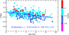Fig. 13.

[Y/Mg] of the thin-disc stars colour-coded by metallicity as a function of age. The continuous line is a fit to the sample of 368 stars. The shadowed area shows a 95% confidence interval for the ordinary least-squares regression.

We also tested the [Y/Al] ratio as a function of age for the thin disc, as a potential age indicator and obtained

$\begin{matrix} {[Y / Al]}_{Thin} = 0.067 (\pm 0.015) - 0.029 (\pm 0.003) \cdot age [Gyr] \end{matrix}$ $\begin{aligned} \mathrm{[Y/Al]_{Thin}}=0.067\,({\pm }0.015)-0.029\,({\pm }0.003)\cdot \mathrm{age\,[Gyr]} \end{aligned}$ (2)

with PCC = −0.42, which is comparable with the [Y/Mg]-age relation. We also targeted other low-scatter light s-process dominated elements as age indicators. Sr also appears to have a good sensitivity to stellar age:

$\begin{matrix} {[Sr / Mg]}_{Thin} = 0.033 (\pm 0.014) - 0.023 (\pm 0.003) \cdot age [Gyr] \end{matrix}$ $\begin{aligned} \mathrm{[Sr/Mg]_{Thin}}= 0.033\,({\pm }0.014)-0.023\,({\pm }0.003)\cdot \mathrm{age\,[Gyr]} \end{aligned}$ (3)

with PPC = −0.39, which makes the [Sr/Mg] abundance ratio a promising age indicator (displayed in Fig. 14). Very recently, Nissen et al. (2020) also tested the sensitivity of Sr in solar-type stars, obtaining a result very similar to that of Y, which is in agreement with our results. Nissen et al. (2020) used the same single Sr I 4607.34 Å line as in our study.

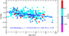Fig. 14.

[Sr/Mg] of the thin-disc stars colour-coded by metallicity as a function of age. The continuous line is a fit to the sample of 368 stars. The shadowed area shows the 95% confidence interval for the ordinary least-squares regression.

When we compare the [Y/Mg] versus age slope obtained in this work to the slope obtained by Nissen et al. (2020), we see a difference of about 0.15 dex in the intercepts even for stars of the same metallicity. In search for the reason, we decided to compute the mean galactocentric distances for the Nissen et al. sample stars and to compare them with those of our sample. Figure 15 shows that in the Nissen et al. (2020) sample, young stars predominantly have larger R_mean. This may cause a larger intercept in the [Y/Mg] and age relation compared to our study and that of Titarenko et al. (2019). Therefore we follow Casali et al. (2020) and Magrini et al. (2021) in concluding that the relations between ages and abundance ratios obtained from samples of stars located in a limited region of the Galaxy cannot be translated into general relations valid for the whole disc. It is worth mentioning that differences in methods used for computing relations and accounting for uncertainties in different studies may also play a role while comparing the results.

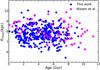Fig. 15.

R_mean and age relation for the sample of thin-disc stars investigated in this work (blue dots) and in Nissen et al. (2020) (magenta diamonds). This figure shows that in the Nissen et al. (2020) sample, young stars predominantly have larger R_mean. This causes a larger intercept in the [Y/Mg] and age relation in Nissen et al. (2020) than in this work.

4.2. [Y/Mg] as age indicator for the thick-disc stars

Our thick-disc sample contains 76 stars with estimated ages. They have a mean ⟨T_eff⟩ = 4715 ± 77 K, ⟨log g⟩ = 2.49 ± 0.25 and ⟨[Fe/H]⟩= − 0.46 ± 0.12, and ages from about 3 to 10 Gyr. Using this sample, we computed a steeper (than the thin-disc stars) negative slope of −0.041 ± 0.013 dex Gyr⁻¹ with a [Y/Mg] intercept of −0.115 ± 0.079 dex, and PPC = −0.35. The [Y/Mg]-age slope given by Titarenko et al. (2019) for the AMBRE sample of 11 thick-disc turn-off stars with ages from about 11.5 to 14.5 Gyr strongly disagrees with our result.

Because of this disagreement, we decided to increase the sample of 76 thick-disc stars by including data from other studies that provided abundances of Y and Mg, as well as ages and separated components of the Galactic disc. Consequently, we included 62 stars (with age uncertainties < 3 Gyr) from Bensby et al. (2014), 88 stars (with age uncertainties < 3 Gyr) from Delgado Mena et al. (2017) and Adibekyan et al. (2012), and 11 stars from Titarenko et al. (2019). The final sample consisted of 237 stars that cover different ranges of metallicity and age.

In Fig. 16 we show the almost negligible [Y/Mg] correlation with age (PCC = −0.04) for the compilation of 237 thick-disc stars:

$\begin{matrix} {[Y / Mg]}_{Thick} = - 0.303 (\pm 0.027) - 0.002 (\pm 0.003) \cdot age [Gyr] . \end{matrix}$ $\begin{aligned} \mathrm{[Y/Mg]_{Thick}}=-0.303\,({\pm }0.027)-0.002\,({\pm }0.003)\cdot \mathrm{age\,[Gyr]}. \end{aligned}$ (4)

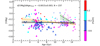Fig. 16.

[Y/Mg] of the thick-disc stars colour-coded by metallicity as a function of age. Our sample stars (triangles) are suplemented by data from Bensby et al. (2014) (dots), Delgado Mena et al. (2018) and Adibekyan et al. (2012) (stars), and Titarenko et al. (2019) (crosses). The black continuous line is a fit to the entire sample of 237 stars. For a comparison, the dashed green line represents the trend taken from Titarenko et al. (2019), who computed it for the AMBRE sample of 11 thick-disc stars; and the dashed yellow line represents the trend that we computed using Bensby et al. (2014) data alone covering the entire investigated age interval. The shadowed areas show the 95% confidence interval for the ordinary least-squares regressions.

In Fig. 16 we show the trend taken from Titarenko et al. (2019) for comparison, who computed this for the AMBRE sample of 11 thick-disc stars, which are all older. This slope disagrees with the results of other old thick-disc stars investigated by Delgado Mena et al. (2017), Bensby et al. (2014), and Adibekyan et al. (2012). Having in mind that the Bensby et al. (2014) sample contains thick-disc stars of a wide range of ages, we computed and displayed a slope based on the Bensby et al. (2014) stellar sample alone. This slope is also quite shallow ([Y/Mg] = −0.168 (±0.040)−0.014 (±0.004)⋅age [Gyr]).

Thus, our study shows that [Y/Mg] can be used as a clock to find stellar ages for the thin-disc stars. The chemical evolution of the thick disc is different, however, and it seems that the [Y/Mg] ratios cannot be used to evaluate the age. Hopefully, the number of thick-disc stars with determined n-capture element abundances will soon increase and a comprehensive study of the thick-disc evolution will proceed.

5. Radial and vertical abundance gradients

The radial and vertical abundance [El/Fe I] gradients were calculated as a function of the mean galactocentric distance (R_mean) and the maximum height from the Galactic plane (|z_max|). R_mean is a better indicator of the stellar birth place than an in situ galactocentric distance. It was used in several previous studies (e.g. Edvardsson et al. 1993; Rocha-Pinto et al. 2004; Trevisan & Barbuy 2014; Adibekyan et al. 2016; Mikolaitis et al. 2019), and could be used more widely, especially while investigating older stars. The target selection strategy in the selected fields was to observe all stars in the selected magnitude and colour range. In this sense, the sample is homogeneous and minimally biased. The targeted sample is magnitude (V < 8 mag) and colour ((B − V) > 0.39) limited, as described in Paper II and Paper III and Sect. 2. The final sample consists of 506 F, G, and K stars distributed in wide atmospheric parameters and age space. The different populations of stars with different metallicities and ages might introduce a bias in the derived abundance radial and vertical gradients. We therefore divided our sample into thin- and thick-disc subsamples in order to avoid the potential bias in analysing gradients.

The resulting values of the radial and vertical abundance gradients for the thin- and thick-disc stars are listed in Tables 6 and 7, respectively. The individual uncertainties of the x- and y-axis data were taken into account when we computed the linear fits with the orthogonal distance regression method using the Kapteyn package (Terlouw & Vogelaar 2014).

Table 6.

Best linear fits to the [El/Fe I]−R_mean and |z_max| distributions in dex kpc⁻¹ for the thin-disc stars.

Table 7.

Best linear fits to the [El/Fe I]−R_mean and |z_max| distributions in dex kpc⁻¹ for the thick-disc stars.

In Fig. 17 we show the radial distribution of [El/Fe I] abundances. The sample stars span the range 5.5 < R_mean < 10 kpc, except for one star at 11.8 kpc.

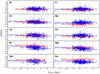Fig. 17.

Elemental-to-iron abundance ratios as a function of the mean galactocentric distances. The blue dots and red triangles represent the thin- and thick-disc stars of our study, respectively. The blue lines are the linear fits for the thin-disc stars and the red lines show the thick-disc stars. The uncertainties in [El/Fe] and R_mean were taken into account while computing the slopes. The 95% confidence intervals for the slopes are shadowed. The dotted lines correspond to the solar mean galactocentric distance.

For the thin-disc stars, the radial [El/Fe] abundance gradients are negligible for the s-process dominated elements and become slightly positive for the elements with stronger r-process domination. The same slightly positive radial [El/Fe] gradients as for the r-process dominated elements in our study were found for α-elements (except odd ones) in Paper II as well as in Li et al. (2018).

Studies of the radial n-capture-to-iron abundance gradients are very scarce so far. We can only search for a broad agreement of our results with several studies of abundance gradients with galactocentric distances (R_gc). da Silva et al. (2016) studied n-capture elements across the Galactic thin disc based on Cepheid variables. Because the Cepheids are young stars, their R_gc may be rather close to their birthplaces and R_mean. da Silva et al. (2016) supplemented their sample of 111 Cepheids with 324 more stars from other studies and found that the [Y/Fe] distribution is flat throughout the entire disc. In our study, we confirm this finding not only based on the whole thin-disc sample of stars and on a subsample of younger ≤4 Gyr stars, but also add another light s-process dominated element strontium. Like in our study, da Silva et al. (2016) also obtained positive [El/Fe] radial gradients for La, Ce, Nd, and Eu. The slopes are rather similar. For [Eu/Fe], they differ just by 0.002 dex kpc⁻¹. More recently, Luck (2018b) also investigated the gradients of n-capture element abundance-to-iron ratios with respect to R_gc for a sample of 435 Cepheids. It is interesting to note that the [Ba/Fe] versus R_gc slope according to this Cepheid sample is also negative, as in our study. [Ba/Fe] is the only n-capture element-to-iron ratio with a negative radial gradient in our sample of stars and in Luck (2018b). Overbeek et al. (2016) investigated trends of Pr, Nd, and Eu to Fe abundance ratios with respect to R_gc using 23 open clusters. As in our study, they found that these elements have positive linear trends with galactocentric radius (the linear regression slopes are of about +0.04 dex kpc⁻¹). They also suggested that the [El/Fe] relation of Pr and Nd, but not Eu, with the galactocentric radius may not be linear because the [El/Fe] of these elements appears to be enhanced around 10 kpc and drop around 12 kpc. Because only a small number of stars lie at these large radial distances, we cannot address this question. For the thick-disc stars, the radial abundance-to-iron slopes are negligible, as was found for α-process elements by Li et al. (2018), even though the production sites of α-elements and s-processes dominated elements are quite different.

In Fig. 18 we present the vertical distribution of the [El/Fe I] abundances. The analysed stars are in the range of 0 < |z_max| < 1.3 kpc, except for one star at 3.73 kpc.

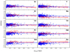Fig. 18.

Elemental-to-iron abundance ratios as a function of the |z_max|. Symbols are the same as in Fig. 17.

For the thin-disc stars, the vertical abundance gradients are predominately negative for the s-process dominated elements and become slightly positive for the r-process dominated elements. For the thick-disc stars, the vertical [El/Fe] gradients for the investigated n-capture elements are negative and become flatter for the r-process dominated elements. The y-intercepts are noticeably larger for the r-process dominated elements.

The vertical [El/Fe] ratio gradients have recently been studied on rather large samples of thin- and thick-disc stars (e.g. Duong et al. 2018; Li et al. 2018; Yan et al. 2019), and for the thin disc in Paper II. Although only α-process elements were investigated in these studies, we can still compare these trends with the r-process dominated element trends in our study because the abundance-to-iron ratios of α-elements and r-process dominated elements are both affected by yields of type II supernovae. It was found that the vertical [α/Fe] trends are positive in the thin disc and negligible in the thick disc. This agrees with the trends of the r-process dominated elements in our study.

Neutron-capture elements are the least well understood in terms of nucleosynthesis and formation environments. These elements can provide much information about the Galactic star formation and enrichment, but observational data are limited, especially for the thick disc.

6. Summary and conclusions

With the aim of testing trends of n-capture element-to-iron abundance ratios versus stellar metallicity, age, mean galactocentric distance, and maximum height from the Galactic plane, we have analysed high-resolution spectra for a sample of 506 F, G, and K spectral-type solar vicinity (V < 8 mag) dwarf, subgiant, and giant stars. The investigated stars are located in the continuous viewing zone of the TESS space mission and in two neighbouring preliminary PLATO space mission fields.

With this work we complement the studies we carried out in Paper I–Paper III, where we provided stellar parameters and abundances of 24 chemical species, which together with those of the present study reach 34 elements, calculated using the same method and instrumentation. The elemental abundance values of the n-capture elements were determined in our work by a differential line-by-line synthesis of spectral lines using MARCS one-dimensional model atmospheres and accounting for the hyperfine-structure effects.

The approximate ranges of atmospheric parameters covered by the stars are the following: 3800 < T_eff < 6900 K, 0.9 < log g < 4.7, and −1.0 < [Fe/H] < +0.5. The stellar ages span from 0.1 to 10 Gyr, R_mean are between 5.5 and 11.8 kpc, and |z_max| are between 0.03 and 3.74 kpc.

The sample contains 424 stars attributed to the Galactic thin disc and 82 stars that belong to the thick disc. We determined abundances of Sr (453 stars), Y (506 stars), Zr I (307 stars), Zr II (476 stars), Ba (504 stars), La (504 stars), Ce (467 stars), Pr (402 stars), Nd (466 stars), Sm (257 stars), and Eu (489 stars).

We compared the observational results with the recent Galactic chemical evolution model by Prantzos et al. (2018). The detailed evaluation of [El/Fe I] versus [Fe I/H] and age trends, and heavy-to-light s-process dominated element abundance ratios versus [Fe I/H] in particular showed that the contribution from the LIMS has to be further investigated and developed. The model agreement with the observations might be better if the convex shape of the model had its maximum not at the [Fe I/H] of −0.4 dex, but at about −0.2 dex, and would start accounting the LIMS input at higher metallicities (about −0.7 dex).

Abundance correlations with age slopes for the thin-disc stars are slightly negative or near zero for the majority of s-process dominated elements. The light s-process elements strontium and yttrium stand out by having a strong negative abundance correlation with age. For the r-process dominated elements, the abundance slopes with age become positive. Similar slopes were also computed in our work using data by Bensby et al. (2014) and Battistini & Bensby (2016), whereas for a sample of solar twins (Spina et al. 2018), all slopes of the same elements were negative. Further studies of the europium abundance versus age gradients deserve special attention.

The neighbouring Galactic thin-disc stars investigated in our study do not show the barium abundance anomaly, like it was found also by Reddy & Lambert (2017) and Marsakov et al. (2016). They do not require the additional i-process as proposed by Cowan & Rose (1977) or Mishenina et al. (2015) to act in the production of barium alone.

The relation obtained from our sample of 424 thin-disc stars is [Y/Mg] = 0.022 (±0.015)−0.027 (±0.003)⋅age [Gyr]. This slope is very similar to the one obtained by Titarenko et al. (2019) for the 325 turn-off thin-disc stars in the AMBRE project.

The thick-disc sample of 76 stars with a mean ⟨[Fe/H]⟩= − 0.51 ± 0.16 might imply a steeper negative slope of [Y/Mg] and age relation. When we increased the sample with data from other studies for the thick disc to 237 stars including larger ages, however, we concluded that the [Y/Mg] and age slope is almost negligible. This proves different chemical evolution histories of the Galactic thin and thick disc components and shows that [Y/Mg] can be used as a clock to determine the age only for the thin-disc stars.

Our sample of 76 thick-disc stars clearly shows a visible decrease in [Eu/Mg] and [r/α] with increasing metallicity compared to the thin-disc stars. This indicates a different chemical evolution of these two Galactic components.

We used the advantage of new possibilities that were opened by the Gaia space mission (Gaia Collaboration 2016, 2018) to determine accurate stellar locations in the Galaxy. We computed slopes of n-capture element abundances with respect to the mean galactocentric distances and distances from the Galactic plane. The mean galactocentric distances of stars are much more informative in indicating stellar birthplaces than the in situ galactocentric distances.

The best linear fits to the [El/Fe I]−R_mean and |z_max| relations (Table 6) show that the radial abundance gradients in the thin disc are negligible for the light s-process dominated elements and become positive for the elements with stronger r-process domination. The vertical abundance gradients are negative for the light s-process dominated elements and become positive for the r-process dominated elements. For the thick disc, the radial abundance-to-iron slopes are negligible, and the vertical slopes are predominantly negative.

The Galactic chemical evolution models still have to be further developed by investigating the roles of yields from rotating massive stars and low- and intermediate-mass stars in producing s-process dominated elements. The relative roles of neutron star mergers and core-collapse supernova in producing r-process dominated elements also await further investigations. Observational data are still scarce for the thick-disc stars. More observational data should be collected for stars of different ages and Galactic locations. The first results from the Gaia-ESO Spectroscopic survey (Magrini et al. 2018), the APOGEE Survey (Cunha et al. 2017), the R-Alliance (Hansen et al. 2018; Sakari et al. 2018), the on-going GALAH (Martell et al. 2017; Griffith et al. 2019) and up-coming WEAVE (Dalton et al. 2016) and 4MOST (de Jong et al. 2019) surveys as well as smaller projects show great potential in bringing new useful observational results. We continue observations in the SPFOT survey as well and plan to compare our expanded observational results with the new GCE models by Grisoni et al. (2020), which appear to fit the thick-disc chemical evolution rather well. With increasing numbers of stars with accurate asteroseismic ages and masses determined from the currently working NASA TESS and the upcoming ESA PLATO space missions, the detailed stellar composition results obtained in the current work and other studies will be very useful for further investigations of Galaxy formation and evolution and for characterising newly found exoplanets.

¹

http://marcs.astro.uu.se/

²

We refer to [Fe I/H] when talking about metallicity.

Acknowledgments

We acknowledge funding from the Research Council of Lithuania (LMTLT) (grant no. LAT-08/2016) and the European Social Fund via the LMTLT (grant no. 09.3.3-LMT-K-712-01-0103). This work has made use of data from the European Space Agency (ESA) mission Gaia (https://www.cosmos.esa.int/gaia), processed by the Gaia Data Processing and Analysis Consortium (DPAC, https://www.cosmos.esa.int/web/gaia/dpac/consortium). Funding for the DPAC has been provided by national institutions, in particular the institutions participating in the Gaia Multilateral Agreement. We gratefully acknowledge Laura Magrini and Nikos Prantzos for providing the GCE models, Alexey Mints for his help with UniDAM, Mark Taylor for his help with TopCat, and Martin Vogelaar for his advises with the Kapteyn Package. We thank the anonymous referee, whose constructive review helped to improve this paper comprehensively. This research made use of the Stilts and Topcat (Taylor 2005, 2006), Astropy (http://www.astropy.org) (Astropy Collaboration 2018), galpy (Bovy 2015) and UniDAM (Mints & Hekker 2017) astronomical tools. We have made extensive use of the NASA ADS and SIMBAD databases.

References

Abbott, B. P., Abbott, R., Abbott, T. D., et al. 2017, ApJ, 848, L12 [Google Scholar]
Adibekyan, V. Z., Sousa, S. G., Santos, N. C., et al. 2012, A&A, 545, A32 [NASA ADS] [CrossRef] [EDP Sciences] [Google Scholar]
Adibekyan, V., Delgado-Mena, E., Figueira, P., et al. 2016, A&A, 592, A87 [NASA ADS] [CrossRef] [EDP Sciences] [Google Scholar]
Adibekyan, V., de Laverny, P., Recio-Blanco, A., et al. 2018, A&A, 619, A130 [CrossRef] [EDP Sciences] [Google Scholar]
Alvarez, R., & Plez, B. 1998, A&A, 330, 1109 [NASA ADS] [Google Scholar]
Arlandini, C., Käppeler, F., Wisshak, K., et al. 1999, ApJ, 525, 886 [NASA ADS] [CrossRef] [Google Scholar]
Asplund, M., Grevesse, N., Sauval, A. J., & Scott, P. 2009, ARA&A, 47, 481 [NASA ADS] [CrossRef] [Google Scholar]
Astropy Collaboration (Price-Whelan, A. M., et al.) 2018, AJ, 156, 123 [Google Scholar]
Bailer-Jones, C. A. L., Rybizki, J., Fouesneau, M., Mantelet, G., & Andrae, R. 2018, VizieR Online Data Catalog: I/347 [Google Scholar]
Battistini, C., & Bensby, T. 2016, A&A, 586, A49 [NASA ADS] [CrossRef] [EDP Sciences] [Google Scholar]
Bensby, T., Feltzing, S., & Oey, M. S. 2014, A&A, 562, A71 [NASA ADS] [CrossRef] [EDP Sciences] [Google Scholar]
Biémont, É., Blagoev, K., Engström, L., et al. 2011, MNRAS, 414, 3350 [NASA ADS] [CrossRef] [Google Scholar]
Biemont, E., Grevesse, N., Hannaford, P., & Lowe, R. M. 1981, ApJ, 248, 867 [NASA ADS] [CrossRef] [Google Scholar]
Bisterzo, S., Travaglio, C., Gallino, R., Wiescher, M., & Käppeler, F. 2014, ApJ, 787, 10 [NASA ADS] [CrossRef] [Google Scholar]
Bisterzo, S., Gallino, R., Käppeler, F., et al. 2015, MNRAS, 449, 506 [NASA ADS] [CrossRef] [Google Scholar]
Bisterzo, S., Travaglio, C., Wiescher, M., Käppeler, F., & Gallino, R. 2017, ApJ, 835, 97 [NASA ADS] [CrossRef] [Google Scholar]
Bovy, J. 2015, ApJS, 216, 29 [Google Scholar]
Burbidge, E. M., Burbidge, G. R., Fowler, W. A., & Hoyle, F. 1957, Rev. Mod. Phys., 29, 547 [NASA ADS] [CrossRef] [Google Scholar]
Busso, M., Gallino, R., & Wasserburg, G. J. 1999, ARA&A, 37, 239 [Google Scholar]
Casali, G., Spina, L., Magrini, L., et al. 2020, A&A, 639, A127 [CrossRef] [EDP Sciences] [Google Scholar]
Clayton, D. D., & Rassbach, M. E. 1967, ApJ, 148, 69 [NASA ADS] [CrossRef] [Google Scholar]
Coc, A., & Vangioni, E. 2017, Int. J. Mod. Phys. E, 26, 1741002 [CrossRef] [Google Scholar]
Corliss, C. H., & Bozman, W. R. 1962, Experimental Transition Probabilities for Spectral Lines of Seventy Elements; Derived from the NBS Tables of Spectral-line Intensities (Washington: US Department of Commerce) [Google Scholar]
Côté, B., Fryer, C. L., Belczynski, K., et al. 2018, ApJ, 855, 99 [NASA ADS] [CrossRef] [Google Scholar]
Côté, B., Eichler, M., Arcones, A., et al. 2019, ApJ, 875, 106 [NASA ADS] [CrossRef] [Google Scholar]
Cowan, J. J., & Rose, W. K. 1977, ApJ, 212, 149 [Google Scholar]
Cowan, J. J., Sneden, C., Lawler, J. E., et al. 2021, Rev. Mod. Phys., 93, 15002 [Google Scholar]
Cowley, C. R., & Corliss, C. H. 1983, MNRAS, 203, 651 [NASA ADS] [CrossRef] [Google Scholar]
Cristallo, S., Abia, C., Straniero, O., & Piersanti, L. 2015, ApJ, 801, 53 [NASA ADS] [CrossRef] [Google Scholar]
Cunha, K., Smith, V. V., Hasselquist, S., et al. 2017, ApJ, 844, 145 [NASA ADS] [CrossRef] [Google Scholar]
Cutri, R. M., Wright, E. L., Conrow, T., et al. 2014, VizieR Online Data Catalog: II/328 [Google Scholar]
Dalton, G., Trager, S., Abrams, D. C., et al. 2016, Proc. SPIE, 9908, 99081G [Google Scholar]
Da Silva, R., Porto de Mello, G. F., Milone, A. C., et al. 2012, A&A, 542, A84 [NASA ADS] [CrossRef] [EDP Sciences] [Google Scholar]
da Silva, R., Lemasle, B., Bono, G., et al. 2016, A&A, 586, A125 [NASA ADS] [CrossRef] [EDP Sciences] [Google Scholar]
Davidson, M. D., Snoek, L. C., Volten, H., & Doenszelmann, A. 1992, A&A, 255, 457 [NASA ADS] [Google Scholar]
de Jong, R. S., Agertz, O., Berbel, A. A., et al. 2019, The Messenger, 175, 3 [NASA ADS] [Google Scholar]
Delgado Mena, E., Tsantaki, M., Adibekyan, V. Z., et al. 2017, A&A, 606, A94 [NASA ADS] [CrossRef] [EDP Sciences] [Google Scholar]
Delgado Mena, E., Adibekyan, V. Z., Figueira, P., et al. 2018, PASP, 130, 094202 [NASA ADS] [CrossRef] [Google Scholar]
Delgado Mena, E., Moya, A., Adibekyan, V., et al. 2019, A&A, 624, A78 [NASA ADS] [CrossRef] [EDP Sciences] [Google Scholar]
Den Hartog, E. A., Lawler, J. E., Sneden, C., & Cowan, J. J. 2003, ApJS, 148, 543 [Google Scholar]
D’Orazi, V., Magrini, L., Randich, S., et al. 2009, ApJ, 693, L31 [NASA ADS] [CrossRef] [Google Scholar]
Duong, L., Freeman, K. C., Asplund, M., et al. 2018, MNRAS, 476, 5216 [NASA ADS] [CrossRef] [Google Scholar]
Edvardsson, B., Andersen, J., Gustafsson, B., et al. 1993, A&A, 500, 391 [NASA ADS] [Google Scholar]
Feltzing, S., Howes, L. M., McMillan, P. J., & Stonkutė, E. 2017, MNRAS, 465, L109 [Google Scholar]
Forsberg, R., Jönsson, H., Ryde, N., & Matteucci, F. 2019, A&A, 631, A113 [CrossRef] [EDP Sciences] [Google Scholar]
Freiburghaus, C., Rosswog, S., & Thielemann, F.-K. 1999, ApJ, 525, L121 [Google Scholar]
Gaia Collaboration (Prusti, T., et al.) 2016, A&A, 595, A1 [NASA ADS] [CrossRef] [EDP Sciences] [Google Scholar]
Gaia Collaboration (Brown, A. G. A., et al.) 2018, A&A, 616, A1 [NASA ADS] [CrossRef] [EDP Sciences] [Google Scholar]
Gallino, R., Arlandini, C., Busso, M., et al. 1998, ApJ, 497, 388 [Google Scholar]
Gratton, R. G., & Sneden, C. 1994, A&A, 287, 927 [NASA ADS] [Google Scholar]
Grevesse, N., Asplund, M., & Sauval, A. J. 2007, Space Sci. Rev., 130, 105 [Google Scholar]
Griffith, E., Johnson, J. A., & Weinberg, D. H. 2019, ApJ, 886, 84 [Google Scholar]
Grisoni, V., Cescutti, G., Matteucci, F., et al. 2020, MNRAS, 492, 2828 [NASA ADS] [CrossRef] [Google Scholar]
Guiglion, G., de Laverny, P., Recio-Blanco, A., & Prantzos, N. 2018, A&A, 619, A143 [NASA ADS] [CrossRef] [EDP Sciences] [Google Scholar]
Gustafsson, B., Edvardsson, B., Eriksson, K., et al. 2008, A&A, 486, 951 [NASA ADS] [CrossRef] [EDP Sciences] [Google Scholar]
Hansen, T. T., Holmbeck, E. M., Beers, T. C., et al. 2018, ApJ, 858, 92 [NASA ADS] [CrossRef] [Google Scholar]
Haynes, C. J., & Kobayashi, C. 2019, MNRAS, 483, 5123 [CrossRef] [Google Scholar]
Heiter, U., Lind, K., Bergemann, M., et al. 2021, A&A, 645, A106 [EDP Sciences] [Google Scholar]
Ivarsson, S., Litzen, U., & Wahlgren, G. M. 2001, Phys. Scr., 64, 455 [Google Scholar]
Jacobson, H. R., & Friel, E. D. 2013, AJ, 145, 107 [NASA ADS] [CrossRef] [Google Scholar]
Jönsson, H., Ryde, N., Nordlander, T., et al. 2017, A&A, 598, A100 [NASA ADS] [CrossRef] [EDP Sciences] [Google Scholar]
Jurgenson, C. A., Fischer, D. A., McCracken, T. M., et al. 2014, Proc. SPIE, 9147, 91477F [Google Scholar]
Jurgenson, C., Fischer, D., McCracken, T., et al. 2016, J. Astron. Instrum., 5, 1650003 [CrossRef] [Google Scholar]
Kappeler, F., Beer, H., & Wisshak, K. 1989, Rep. Progr. Phys., 52, 945 [Google Scholar]
Käppeler, F., Gallino, R., Bisterzo, S., & Aoki, W. 2011, Rev. Mod. Phys., 83, 157 [Google Scholar]
Karakas, A. I. 2014, in Setting the Scene for Gaia and LAMOST, eds. S. Feltzing, G. Zhao, N. A. Walton, & P. Whitelock, IAU Symp., 298, 142 [Google Scholar]
Katz, D., Sartoretti, P., Cropper, M., et al. 2019, A&A, 622, A205 [NASA ADS] [CrossRef] [EDP Sciences] [Google Scholar]
Kobayashi, C., Karakas, A. I., & Lugaro, M. 2020, ApJ, 900, 179 [CrossRef] [Google Scholar]
Korotin, S. A., Andrievsky, S. M., Hansen, C. J., et al. 2015, A&A, 581, A70 [NASA ADS] [CrossRef] [EDP Sciences] [Google Scholar]
Lamb, S. A., Howard, W. M., Truran, J. W., & Iben, I., Jr. 1977, ApJ, 217, 213 [NASA ADS] [CrossRef] [Google Scholar]
Lawler, J. E., Bonvallet, G., & Sneden, C. 2001a, ApJ, 556, 452 [NASA ADS] [CrossRef] [Google Scholar]
Lawler, J. E., Wickliffe, M. E., den Hartog, E. A., & Sneden, C. 2001b, ApJ, 563, 1075 [CrossRef] [Google Scholar]
Lawler, J. E., Den Hartog, E. A., Sneden, C., & Cowan, J. J. 2006, ApJS, 162, 227 [NASA ADS] [CrossRef] [Google Scholar]
Lawler, J. E., Sneden, C., Cowan, J. J., Ivans, I. I., & Den Hartog, E. A. 2009, ApJS, 182, 51 [Google Scholar]
Li, R., Chatelain, R., Holt, R. A., et al. 2007, Phys. Scr., 76, 577 [Google Scholar]
Li, C., Zhao, G., Zhai, M., & Jia, Y. 2018, ApJ, 860, 53 [NASA ADS] [CrossRef] [Google Scholar]
Liu, S., Shi, J., & Wu, Z. 2020, ApJ, 896, 64 [Google Scholar]
Luck, R. E. 2017, AJ, 153, 21 [Google Scholar]
Luck, R. E. 2018a, AJ, 155, 111 [NASA ADS] [CrossRef] [Google Scholar]
Luck, R. E. 2018b, AJ, 156, 171 [NASA ADS] [CrossRef] [Google Scholar]
Luri, X., Brown, A. G. A., Sarro, L. M., et al. 2018, A&A, 616, A9 [NASA ADS] [CrossRef] [EDP Sciences] [Google Scholar]
Magrini, L., Spina, L., Randich, S., et al. 2018, A&A, 617, A106 [NASA ADS] [CrossRef] [EDP Sciences] [Google Scholar]
Magrini, L., Vescovi, D., Casali, G., et al. 2021, A&A, 646, L2 [EDP Sciences] [Google Scholar]
Maiorca, E., Magrini, L., Busso, M., et al. 2012, ApJ, 747, 53 [Google Scholar]
Marsakov, V. A., Gozha, M. L., Koval’, V. V., & Shpigel’, L. V. 2016, Astron. Rep., 60, 61 [Google Scholar]
Martell, S. L., Sharma, S., Buder, S., et al. 2017, MNRAS, 465, 3203 [Google Scholar]
Mashonkina, L., & Gehren, T. 2001, A&A, 376, 232 [NASA ADS] [CrossRef] [EDP Sciences] [Google Scholar]
Mashonkina, L., Gehren, T., Travaglio, C., & Borkova, T. 2003, A&A, 397, 275 [NASA ADS] [CrossRef] [EDP Sciences] [Google Scholar]
Matteucci, F., Romano, D., Arcones, A., Korobkin, O., & Rosswog, S. 2014, MNRAS, 438, 2177 [NASA ADS] [CrossRef] [Google Scholar]
Meggers, W. F., Corliss, C. H., & Scribner, B. F. 1975, Tables of Spectral-line Intensities. Part I, II_– Arranged by Elements [Google Scholar]
Miglio, A., Chiappini, C., Mosser, B., et al. 2017, Astron. Nachr., 338, 644 [NASA ADS] [CrossRef] [Google Scholar]
Mikolaitis, Š., Tautvaišienė, G., Drazdauskas, A., et al. 2018, PASP, 130, 074202 [CrossRef] [Google Scholar]
Mikolaitis, Š., Drazdauskas, A., Minkevičiūtė, R., et al. 2019, A&A, 628, A49 [EDP Sciences] [Google Scholar]
Miles, B. M., & Wiese, W. L. 1969, At. Data, 1, 1 [Google Scholar]
Mints, A., & Hekker, S. 2017, A&A, 604, A108 [NASA ADS] [CrossRef] [EDP Sciences] [Google Scholar]
Mishenina, T. V., Pignatari, M., Korotin, S. A., et al. 2013, A&A, 552, A128 [NASA ADS] [CrossRef] [EDP Sciences] [Google Scholar]
Mishenina, T., Pignatari, M., Carraro, G., et al. 2015, MNRAS, 446, 3651 [Google Scholar]
Mishenina, T., Pignatari, M., Gorbaneva, T., et al. 2019, MNRAS, 484, 3846 [Google Scholar]
Nishimura, S., Kotake, K., Hashimoto, M.-A., et al. 2006, ApJ, 642, 410 [NASA ADS] [CrossRef] [Google Scholar]
Nissen, P. E. 2015, A&A, 579, A52 [NASA ADS] [CrossRef] [EDP Sciences] [Google Scholar]
Nissen, P. E. 2016, A&A, 593, A65 [NASA ADS] [CrossRef] [EDP Sciences] [Google Scholar]
Nissen, P. E., Silva Aguirre, V., Christensen-Dalsgaard, J., et al. 2017, A&A, 608, A112 [NASA ADS] [CrossRef] [EDP Sciences] [Google Scholar]
Nissen, P. E., Christensen-Dalsgaard, J., Mosumgaard, J. R., et al. 2020, A&A, 640, A81 [CrossRef] [EDP Sciences] [Google Scholar]
Overbeek, J. C., Friel, E. D., & Jacobson, H. R. 2016, ApJ, 824, 75 [NASA ADS] [CrossRef] [Google Scholar]
Pagel, B. E. J., & Tautvaisiene, G. 1997, MNRAS, 288, 108 [NASA ADS] [CrossRef] [Google Scholar]
Parkinson, J. H. 1976, Philos. Trans. R. Soc. London Ser. A, 281, 375 [Google Scholar]
Peters, J. G. 1968, ApJ, 154, 225 [NASA ADS] [CrossRef] [Google Scholar]
Pignatari, M., Gallino, R., Heil, M., et al. 2010, ApJ, 710, 1557 [NASA ADS] [CrossRef] [Google Scholar]
Prantzos, N., Abia, C., Limongi, M., Chieffi, A., & Cristallo, S. 2018, MNRAS, 476, 3432 [Google Scholar]
Prantzos, N., Abia, C., Cristallo, S., Limongi, M., & Chieffi, A. 2020, MNRAS, 491, 1832 [Google Scholar]
Rauer, H., Catala, C., Aerts, C., et al. 2014, Exp. Astron., 38, 249 [Google Scholar]
Reddy, A. B. S., & Lambert, D. L. 2017, ApJ, 845, 151 [Google Scholar]
Ricker, G. R., Winn, J. N., Vanderspek, R., et al. 2015, J. Astron. Telesc. Instrum. Syst., 1, 014003 [Google Scholar]
Rocha-Pinto, H. J., Flynn, C., Scalo, J., et al. 2004, A&A, 423, 517 [NASA ADS] [CrossRef] [EDP Sciences] [Google Scholar]
Sakari, C. M., Placco, V. M., Farrell, E. M., et al. 2018, ApJ, 868, 110 [NASA ADS] [CrossRef] [Google Scholar]
Schönrich, R. A., & Weinberg, D. H. 2019, MNRAS, 487, 580 [NASA ADS] [CrossRef] [Google Scholar]
Shen, S., Cooke, R. J., Ramirez-Ruiz, E., et al. 2015, ApJ, 807, 115 [NASA ADS] [CrossRef] [Google Scholar]
Siegel, D. M., Barnes, J., & Metzger, B. D. 2019, Nature, 569, 241 [Google Scholar]
Skrutskie, M. F., Cutri, R. M., Stiening, R., et al. 2006, AJ, 131, 1163 [NASA ADS] [CrossRef] [Google Scholar]
Slumstrup, D., Grundahl, F., Brogaard, K., et al. 2017, A&A, 604, L8 [NASA ADS] [CrossRef] [EDP Sciences] [Google Scholar]
Sneden, C. A. 1973, PhD Thesis, The University of Texas at Austin, USA [Google Scholar]
Sneden, C., Cowan, J. J., & Gallino, R. 2008, ARA&A, 46, 241 [NASA ADS] [CrossRef] [EDP Sciences] [Google Scholar]
Sneden, C., Lawler, J. E., Cowan, J. J., Ivans, I. I., & Den Hartog, E. A. 2009, ApJS, 182, 80 [Google Scholar]
Spina, L., Meléndez, J., Karakas, A. I., et al. 2016, A&A, 593, A125 [NASA ADS] [CrossRef] [EDP Sciences] [Google Scholar]
Spina, L., Meléndez, J., Karakas, A. I., et al. 2018, MNRAS, 474, 2580 [NASA ADS] [Google Scholar]
Spina, L., Nordlander, T., Casey, A. R., et al. 2020, ApJ, 895, 52 [Google Scholar]
Sullivan, P. W., Winn, J. N., Berta-Thompson, Z. K., et al. 2015, ApJ, 809, 77 [NASA ADS] [CrossRef] [Google Scholar]
Surman, R., McLaughlin, G. C., Ruffert, M., Janka, H.-T., & Hix, W. R. 2008, ApJ, 679, L117 [Google Scholar]
Tautvaišienė, G., Mikolaitis, Š., Drazdauskas, A., et al. 2020, ApJS, 248, 19 [Google Scholar]
Taylor, M. B. 2005, in Astronomical Data Analysis Software and Systems XIV, eds. P. Shopbell, M. Britton, & R. Ebert, ASP Conf. Ser., 347, 29 [Google Scholar]
Taylor, M. B. 2006, in Astronomical Data Analysis Software and Systems XV, eds. C. Gabriel, C. Arviset, D. Ponz, & S. Enrique, ASP Conf. Ser., 351, 666 [Google Scholar]
Terlouw, J. P., & Vogelaar, M. G. R. 2014, Kapteyn Package, version 2.3b3, Kapteyn Astronomical Institute, Groningen, http://www.astro.rug.nl/software/kapteyn/ [Google Scholar]
Thielemann, F. K., Eichler, M., Panov, I. V., & Wehmeyer, B. 2017, Annu. Rev. Nucl. Part. Sci., 67, 253 [Google Scholar]
Titarenko, A., Recio-Blanco, A., de Laverny, P., Hayden, M., & Guiglion, G. 2019, A&A, 622, A59 [NASA ADS] [CrossRef] [EDP Sciences] [Google Scholar]
Travaglio, C., Gallino, R., Busso, M., & Gratton, R. 2001, ApJ, 549, 346 [NASA ADS] [CrossRef] [Google Scholar]
Travaglio, C., Gallino, R., Arnone, E., et al. 2004, ApJ, 601, 864 [NASA ADS] [CrossRef] [Google Scholar]
Trevisan, M., & Barbuy, B. 2014, A&A, 570, A22 [NASA ADS] [CrossRef] [EDP Sciences] [Google Scholar]
Trippella, O., Busso, M., Palmerini, S., Maiorca, E., & Nucci, M. C. 2016, ApJ, 818, 125 [NASA ADS] [CrossRef] [PubMed] [Google Scholar]
Tucci Maia, M., Ramírez, I., Meléndez, J., et al. 2016, A&A, 590, A32 [NASA ADS] [CrossRef] [EDP Sciences] [Google Scholar]
Watson, D., Hansen, C. J., Selsing, J., et al. 2019, Nature, 574, 497 [NASA ADS] [CrossRef] [Google Scholar]
Woosley, S. E., Wilson, J. R., Mathews, G. J., Hoffman, R. D., & Meyer, B. S. 1994, ApJ, 433, 229 [NASA ADS] [CrossRef] [Google Scholar]
Yan, Y., Du, C., Liu, S., et al. 2019, ApJ, 880, 36 [Google Scholar]
Yong, D., Carney, B. W., & Friel, E. D. 2012, AJ, 144, 95 [NASA ADS] [CrossRef] [Google Scholar]
Zhao, G., Mashonkina, L., Yan, H. L., et al. 2016, ApJ, 833, 225 [Google Scholar]

All Tables

Table 1.

Solar abundances of the investigated chemical elements as determined using two different resolution modes of the VUES spectrograph and values by Asplund et al. (2009).

In the text

Table 2.

Sensitivity of abundances to the median values of uncertainties in atmospheric parameters and random uncertainties.

In the text

Table 3.

Atmospheric parameters and abundances of neutron-capture elements.

In the text

Table 4.

Solar percentage of s-process input for the n-capture elements.

In the text

Table 5.

Best linear fits to the [El/Fe I]−age distributions in dex Gyr⁻¹ and the Pearson correlation coefficients for the thin disc stars and comparison with other works.

In the text

Table 6.

Best linear fits to the [El/Fe I]−R_mean and |z_max| distributions in dex kpc⁻¹ for the thin-disc stars.

In the text

Table 7.

Best linear fits to the [El/Fe I]−R_mean and |z_max| distributions in dex kpc⁻¹ for the thick-disc stars.

In the text

All Figures

	Fig. 1. Positions of all selected programme stars (black dots) observed from the Molėtai Astronomical Observatory in Lithuania. The violet areas denote the preliminary PLATO fields and all observed dwarf stars, while the red area marks the continuous viewing zone of the TESS telescope.
In the text

	Fig. 2. Investigated stars in a surface gravity and effective temperature diagram showing a density estimation and bivariate distribution.
In the text

	Fig. 3. Observed rms scatter around the median [El/Fe] abundance (grey lines) and expected uncertainties (red lines) in four metallicity and age bins (thin vertical lines). The open circles at every bin are placed at the median value of the [Fe/H] or age of the corresponding bin.
In the text

	Fig. 4. Uncertainties on the abundance ratios as a function of T_eff, log g, and [Fe/H]. The blue dots represent the thin-disc and the red triangles represent the thick-disc stars. See Sect. 2.5 for details of how the uncertainties have been evaluated.
In the text

	Fig. 5. Elemental abundance trends relative to [Fe I/H]. The blue dots represent the thin-disc stars, and red triangles indicate the thick-disc stars. The continuous lines show the models by Prantzos et al. (2018) (cyan) and Pagel & Tautvaisiene (1997) (black).
In the text

	Fig. 6. Ratio of heavy (Ba, La, Ce, Nd) and light (Sr, Y, Zr) s-process dominated element abundances with respect to [Fe I/H] compared with the GCE model predictions by Prantzos et al. (2018) (cyan line) and the thin-disc model by Pagel & Tautvaisiene (1997) (black line). Our results are marked as blue circles for the thin-disc and as red triangles for the thick-disc stars.
In the text

	Fig. 7. [Eu/Ba] ratio with respect to [Fe I/H]. Symbols are the same as in Fig. 6. The dotted line and the shadowed area of ±0.1 dex uncertainty represent a pure r-process ratio derived using the percentages of Bisterzo et al. (2014) and the solar abundances of Grevesse et al. (2007).
In the text

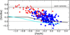	Fig. 8. [Sm/Ba] ratio with respect to [Fe I/H]. Symbols are the same as in Fig. 7.
In the text

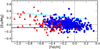	Fig. 9. [Eu/Mg] ratio with respect to [Fe I/H]. Symbols are the same as in Fig. 6.
In the text

Fig. 10.

Elemental-to-iron abundance ratios as a function of age. The blue dots and red triangles represent the thin- and thick-disc stars of our study, respectively. The green lines represent the models by Maiorca et al. (2012) and the cyan lines those by Prantzos et al. (2018). The blue lines are the linear fits for the thin-disc stars of this work and the red lines show the thick-disc stars, with a 95% confidence interval for the ordinary least-squares regressions. The vertical dashed lines indicate the adopted age of the Sun (4.53 Gyr).

In the text

Fig. 11.

Compilation of [El/Fe I] trends as a function of age for the thin-disc stars. The continuous purple lines represent the r-process dominated elements Eu, Sm, and Pr. The thick dash-dotted line is an averaged trend of these element-to-iron abundance ratios. The continuous blue lines represent the s-process dominated elements Y, Sr, and Ba. The thick dash-dotted line is an averaged trend of these element-to-iron abundance ratios. The grey continuous lines are for elements with negligible [El/Fe I] age trends (Nd, Ce, La, and Zr). The continuous magenta line represents the [Mg/Fe I] age correlation. The shadowed areas show the 95% confidence interval for the regressions. The vertical dashed line marks the solar age.

In the text

Fig. 12.

Compilation of [El/FeI] trends as a function of age for the thick-disc stars. The continuous purple line represents the r-process dominated element Sm, which alone shows a slight trend, but with a quite low accuracy. The continuous blue line represents the s-process dominated element Y, which has a more noticeable trend than the others. The grey continuous lines are for elements with negligible trends of [El/FeI] vs. age. The continuous magenta line represents the [Mg/FeI] age correlation. The shadowed areas show the 95% confidence interval for the regressions. The vertical dashed line marks the solar age.

In the text

	Fig. 13. [Y/Mg] of the thin-disc stars colour-coded by metallicity as a function of age. The continuous line is a fit to the sample of 368 stars. The shadowed area shows a 95% confidence interval for the ordinary least-squares regression.
In the text

	Fig. 14. [Sr/Mg] of the thin-disc stars colour-coded by metallicity as a function of age. The continuous line is a fit to the sample of 368 stars. The shadowed area shows the 95% confidence interval for the ordinary least-squares regression.
In the text

	Fig. 15. R_mean and age relation for the sample of thin-disc stars investigated in this work (blue dots) and in Nissen et al. (2020) (magenta diamonds). This figure shows that in the Nissen et al. (2020) sample, young stars predominantly have larger R_mean. This causes a larger intercept in the [Y/Mg] and age relation in Nissen et al. (2020) than in this work.
In the text

Fig. 16.

[Y/Mg] of the thick-disc stars colour-coded by metallicity as a function of age. Our sample stars (triangles) are suplemented by data from Bensby et al. (2014) (dots), Delgado Mena et al. (2018) and Adibekyan et al. (2012) (stars), and Titarenko et al. (2019) (crosses). The black continuous line is a fit to the entire sample of 237 stars. For a comparison, the dashed green line represents the trend taken from Titarenko et al. (2019), who computed it for the AMBRE sample of 11 thick-disc stars; and the dashed yellow line represents the trend that we computed using Bensby et al. (2014) data alone covering the entire investigated age interval. The shadowed areas show the 95% confidence interval for the ordinary least-squares regressions.

In the text

Fig. 17.

Elemental-to-iron abundance ratios as a function of the mean galactocentric distances. The blue dots and red triangles represent the thin- and thick-disc stars of our study, respectively. The blue lines are the linear fits for the thin-disc stars and the red lines show the thick-disc stars. The uncertainties in [El/Fe] and R_mean were taken into account while computing the slopes. The 95% confidence intervals for the slopes are shadowed. The dotted lines correspond to the solar mean galactocentric distance.

In the text

	Fig. 18. Elemental-to-iron abundance ratios as a function of the \|z_max\|. Symbols are the same as in Fig. 17.
In the text

Current usage metrics show cumulative count of Article Views (full-text article views including HTML views, PDF and ePub downloads, according to the available data) and Abstracts Views on Vision4Press platform.

Data correspond to usage on the plateform after 2015. The current usage metrics is available 48-96 hours after online publication and is updated daily on week days.

Initial download of the metrics may take a while.

[1] Abbott, B. P., Abbott, R., Abbott, T. D., et al. 2017, ApJ, 848, L12 [Google Scholar]

[2] Adibekyan, V. Z., Sousa, S. G., Santos, N. C., et al. 2012, A&A, 545, A32 [NASA ADS] [CrossRef] [EDP Sciences] [Google Scholar]

[3] Adibekyan, V., Delgado-Mena, E., Figueira, P., et al. 2016, A&A, 592, A87 [NASA ADS] [CrossRef] [EDP Sciences] [Google Scholar]

[4] Adibekyan, V., de Laverny, P., Recio-Blanco, A., et al. 2018, A&A, 619, A130 [CrossRef] [EDP Sciences] [Google Scholar]

[5] Alvarez, R., & Plez, B. 1998, A&A, 330, 1109 [NASA ADS] [Google Scholar]

[6] Arlandini, C., Käppeler, F., Wisshak, K., et al. 1999, ApJ, 525, 886 [NASA ADS] [CrossRef] [Google Scholar]

[7] Asplund, M., Grevesse, N., Sauval, A. J., & Scott, P. 2009, ARA&A, 47, 481 [NASA ADS] [CrossRef] [Google Scholar]

[8] Astropy Collaboration (Price-Whelan, A. M., et al.) 2018, AJ, 156, 123 [Google Scholar]

[9] Bailer-Jones, C. A. L., Rybizki, J., Fouesneau, M., Mantelet, G., & Andrae, R. 2018, VizieR Online Data Catalog: I/347 [Google Scholar]

[10] Battistini, C., & Bensby, T. 2016, A&A, 586, A49 [NASA ADS] [CrossRef] [EDP Sciences] [Google Scholar]

[11] Bensby, T., Feltzing, S., & Oey, M. S. 2014, A&A, 562, A71 [NASA ADS] [CrossRef] [EDP Sciences] [Google Scholar]

[12] Biémont, É., Blagoev, K., Engström, L., et al. 2011, MNRAS, 414, 3350 [NASA ADS] [CrossRef] [Google Scholar]

[13] Biemont, E., Grevesse, N., Hannaford, P., & Lowe, R. M. 1981, ApJ, 248, 867 [NASA ADS] [CrossRef] [Google Scholar]

[14] Bisterzo, S., Travaglio, C., Gallino, R., Wiescher, M., & Käppeler, F. 2014, ApJ, 787, 10 [NASA ADS] [CrossRef] [Google Scholar]

[15] Bisterzo, S., Gallino, R., Käppeler, F., et al. 2015, MNRAS, 449, 506 [NASA ADS] [CrossRef] [Google Scholar]

[16] Bisterzo, S., Travaglio, C., Wiescher, M., Käppeler, F., & Gallino, R. 2017, ApJ, 835, 97 [NASA ADS] [CrossRef] [Google Scholar]

[17] Bovy, J. 2015, ApJS, 216, 29 [Google Scholar]

[18] Burbidge, E. M., Burbidge, G. R., Fowler, W. A., & Hoyle, F. 1957, Rev. Mod. Phys., 29, 547 [NASA ADS] [CrossRef] [Google Scholar]

[19] Busso, M., Gallino, R., & Wasserburg, G. J. 1999, ARA&A, 37, 239 [Google Scholar]

[20] Casali, G., Spina, L., Magrini, L., et al. 2020, A&A, 639, A127 [CrossRef] [EDP Sciences] [Google Scholar]

[21] Clayton, D. D., & Rassbach, M. E. 1967, ApJ, 148, 69 [NASA ADS] [CrossRef] [Google Scholar]

[22] Coc, A., & Vangioni, E. 2017, Int. J. Mod. Phys. E, 26, 1741002 [CrossRef] [Google Scholar]

[23] Corliss, C. H., & Bozman, W. R. 1962, Experimental Transition Probabilities for Spectral Lines of Seventy Elements; Derived from the NBS Tables of Spectral-line Intensities (Washington: US Department of Commerce) [Google Scholar]

[24] Côté, B., Fryer, C. L., Belczynski, K., et al. 2018, ApJ, 855, 99 [NASA ADS] [CrossRef] [Google Scholar]

[25] Côté, B., Eichler, M., Arcones, A., et al. 2019, ApJ, 875, 106 [NASA ADS] [CrossRef] [Google Scholar]

[26] Cowan, J. J., & Rose, W. K. 1977, ApJ, 212, 149 [Google Scholar]

[27] Cowan, J. J., Sneden, C., Lawler, J. E., et al. 2021, Rev. Mod. Phys., 93, 15002 [Google Scholar]

[28] Cowley, C. R., & Corliss, C. H. 1983, MNRAS, 203, 651 [NASA ADS] [CrossRef] [Google Scholar]

[29] Cristallo, S., Abia, C., Straniero, O., & Piersanti, L. 2015, ApJ, 801, 53 [NASA ADS] [CrossRef] [Google Scholar]

[30] Cunha, K., Smith, V. V., Hasselquist, S., et al. 2017, ApJ, 844, 145 [NASA ADS] [CrossRef] [Google Scholar]

[31] Cutri, R. M., Wright, E. L., Conrow, T., et al. 2014, VizieR Online Data Catalog: II/328 [Google Scholar]

[32] Dalton, G., Trager, S., Abrams, D. C., et al. 2016, Proc. SPIE, 9908, 99081G [Google Scholar]

[33] Da Silva, R., Porto de Mello, G. F., Milone, A. C., et al. 2012, A&A, 542, A84 [NASA ADS] [CrossRef] [EDP Sciences] [Google Scholar]

[34] da Silva, R., Lemasle, B., Bono, G., et al. 2016, A&A, 586, A125 [NASA ADS] [CrossRef] [EDP Sciences] [Google Scholar]

[35] Davidson, M. D., Snoek, L. C., Volten, H., & Doenszelmann, A. 1992, A&A, 255, 457 [NASA ADS] [Google Scholar]

[36] de Jong, R. S., Agertz, O., Berbel, A. A., et al. 2019, The Messenger, 175, 3 [NASA ADS] [Google Scholar]

[37] Delgado Mena, E., Tsantaki, M., Adibekyan, V. Z., et al. 2017, A&A, 606, A94 [NASA ADS] [CrossRef] [EDP Sciences] [Google Scholar]

[38] Delgado Mena, E., Adibekyan, V. Z., Figueira, P., et al. 2018, PASP, 130, 094202 [NASA ADS] [CrossRef] [Google Scholar]

[39] Delgado Mena, E., Moya, A., Adibekyan, V., et al. 2019, A&A, 624, A78 [NASA ADS] [CrossRef] [EDP Sciences] [Google Scholar]

[40] Den Hartog, E. A., Lawler, J. E., Sneden, C., & Cowan, J. J. 2003, ApJS, 148, 543 [Google Scholar]

[41] D’Orazi, V., Magrini, L., Randich, S., et al. 2009, ApJ, 693, L31 [NASA ADS] [CrossRef] [Google Scholar]

[42] Duong, L., Freeman, K. C., Asplund, M., et al. 2018, MNRAS, 476, 5216 [NASA ADS] [CrossRef] [Google Scholar]

[43] Edvardsson, B., Andersen, J., Gustafsson, B., et al. 1993, A&A, 500, 391 [NASA ADS] [Google Scholar]

[44] Feltzing, S., Howes, L. M., McMillan, P. J., & Stonkutė, E. 2017, MNRAS, 465, L109 [Google Scholar]

[45] Forsberg, R., Jönsson, H., Ryde, N., & Matteucci, F. 2019, A&A, 631, A113 [CrossRef] [EDP Sciences] [Google Scholar]

[46] Freiburghaus, C., Rosswog, S., & Thielemann, F.-K. 1999, ApJ, 525, L121 [Google Scholar]

[47] Gaia Collaboration (Prusti, T., et al.) 2016, A&A, 595, A1 [NASA ADS] [CrossRef] [EDP Sciences] [Google Scholar]

[48] Gaia Collaboration (Brown, A. G. A., et al.) 2018, A&A, 616, A1 [NASA ADS] [CrossRef] [EDP Sciences] [Google Scholar]

[49] Gallino, R., Arlandini, C., Busso, M., et al. 1998, ApJ, 497, 388 [Google Scholar]

[50] Gratton, R. G., & Sneden, C. 1994, A&A, 287, 927 [NASA ADS] [Google Scholar]

[51] Grevesse, N., Asplund, M., & Sauval, A. J. 2007, Space Sci. Rev., 130, 105 [Google Scholar]

[52] Griffith, E., Johnson, J. A., & Weinberg, D. H. 2019, ApJ, 886, 84 [Google Scholar]

[53] Grisoni, V., Cescutti, G., Matteucci, F., et al. 2020, MNRAS, 492, 2828 [NASA ADS] [CrossRef] [Google Scholar]

[54] Guiglion, G., de Laverny, P., Recio-Blanco, A., & Prantzos, N. 2018, A&A, 619, A143 [NASA ADS] [CrossRef] [EDP Sciences] [Google Scholar]

[55] Gustafsson, B., Edvardsson, B., Eriksson, K., et al. 2008, A&A, 486, 951 [NASA ADS] [CrossRef] [EDP Sciences] [Google Scholar]

[56] Hansen, T. T., Holmbeck, E. M., Beers, T. C., et al. 2018, ApJ, 858, 92 [NASA ADS] [CrossRef] [Google Scholar]

[57] Haynes, C. J., & Kobayashi, C. 2019, MNRAS, 483, 5123 [CrossRef] [Google Scholar]

[58] Heiter, U., Lind, K., Bergemann, M., et al. 2021, A&A, 645, A106 [EDP Sciences] [Google Scholar]

[59] Ivarsson, S., Litzen, U., & Wahlgren, G. M. 2001, Phys. Scr., 64, 455 [Google Scholar]

[60] Jacobson, H. R., & Friel, E. D. 2013, AJ, 145, 107 [NASA ADS] [CrossRef] [Google Scholar]

[61] Jönsson, H., Ryde, N., Nordlander, T., et al. 2017, A&A, 598, A100 [NASA ADS] [CrossRef] [EDP Sciences] [Google Scholar]

[62] Jurgenson, C. A., Fischer, D. A., McCracken, T. M., et al. 2014, Proc. SPIE, 9147, 91477F [Google Scholar]

[63] Jurgenson, C., Fischer, D., McCracken, T., et al. 2016, J. Astron. Instrum., 5, 1650003 [CrossRef] [Google Scholar]

[64] Kappeler, F., Beer, H., & Wisshak, K. 1989, Rep. Progr. Phys., 52, 945 [Google Scholar]

[65] Käppeler, F., Gallino, R., Bisterzo, S., & Aoki, W. 2011, Rev. Mod. Phys., 83, 157 [Google Scholar]

[66] Karakas, A. I. 2014, in Setting the Scene for Gaia and LAMOST, eds. S. Feltzing, G. Zhao, N. A. Walton, & P. Whitelock, IAU Symp., 298, 142 [Google Scholar]

[67] Katz, D., Sartoretti, P., Cropper, M., et al. 2019, A&A, 622, A205 [NASA ADS] [CrossRef] [EDP Sciences] [Google Scholar]

[68] Kobayashi, C., Karakas, A. I., & Lugaro, M. 2020, ApJ, 900, 179 [CrossRef] [Google Scholar]

[69] Korotin, S. A., Andrievsky, S. M., Hansen, C. J., et al. 2015, A&A, 581, A70 [NASA ADS] [CrossRef] [EDP Sciences] [Google Scholar]

[70] Lamb, S. A., Howard, W. M., Truran, J. W., & Iben, I., Jr. 1977, ApJ, 217, 213 [NASA ADS] [CrossRef] [Google Scholar]

[71] Lawler, J. E., Bonvallet, G., & Sneden, C. 2001a, ApJ, 556, 452 [NASA ADS] [CrossRef] [Google Scholar]

[72] Lawler, J. E., Wickliffe, M. E., den Hartog, E. A., & Sneden, C. 2001b, ApJ, 563, 1075 [CrossRef] [Google Scholar]

[73] Lawler, J. E., Den Hartog, E. A., Sneden, C., & Cowan, J. J. 2006, ApJS, 162, 227 [NASA ADS] [CrossRef] [Google Scholar]

[74] Lawler, J. E., Sneden, C., Cowan, J. J., Ivans, I. I., & Den Hartog, E. A. 2009, ApJS, 182, 51 [Google Scholar]

[75] Li, R., Chatelain, R., Holt, R. A., et al. 2007, Phys. Scr., 76, 577 [Google Scholar]

[76] Li, C., Zhao, G., Zhai, M., & Jia, Y. 2018, ApJ, 860, 53 [NASA ADS] [CrossRef] [Google Scholar]

[77] Liu, S., Shi, J., & Wu, Z. 2020, ApJ, 896, 64 [Google Scholar]

[78] Luck, R. E. 2017, AJ, 153, 21 [Google Scholar]

[79] Luck, R. E. 2018a, AJ, 155, 111 [NASA ADS] [CrossRef] [Google Scholar]

[80] Luck, R. E. 2018b, AJ, 156, 171 [NASA ADS] [CrossRef] [Google Scholar]

[81] Luri, X., Brown, A. G. A., Sarro, L. M., et al. 2018, A&A, 616, A9 [NASA ADS] [CrossRef] [EDP Sciences] [Google Scholar]

[82] Magrini, L., Spina, L., Randich, S., et al. 2018, A&A, 617, A106 [NASA ADS] [CrossRef] [EDP Sciences] [Google Scholar]

[83] Magrini, L., Vescovi, D., Casali, G., et al. 2021, A&A, 646, L2 [EDP Sciences] [Google Scholar]

[84] Maiorca, E., Magrini, L., Busso, M., et al. 2012, ApJ, 747, 53 [Google Scholar]

[85] Marsakov, V. A., Gozha, M. L., Koval’, V. V., & Shpigel’, L. V. 2016, Astron. Rep., 60, 61 [Google Scholar]

[86] Martell, S. L., Sharma, S., Buder, S., et al. 2017, MNRAS, 465, 3203 [Google Scholar]

[87] Mashonkina, L., & Gehren, T. 2001, A&A, 376, 232 [NASA ADS] [CrossRef] [EDP Sciences] [Google Scholar]

[88] Mashonkina, L., Gehren, T., Travaglio, C., & Borkova, T. 2003, A&A, 397, 275 [NASA ADS] [CrossRef] [EDP Sciences] [Google Scholar]

[89] Matteucci, F., Romano, D., Arcones, A., Korobkin, O., & Rosswog, S. 2014, MNRAS, 438, 2177 [NASA ADS] [CrossRef] [Google Scholar]

[90] Meggers, W. F., Corliss, C. H., & Scribner, B. F. 1975, Tables of Spectral-line Intensities. Part I, II_– Arranged by Elements [Google Scholar]

[91] Miglio, A., Chiappini, C., Mosser, B., et al. 2017, Astron. Nachr., 338, 644 [NASA ADS] [CrossRef] [Google Scholar]

[92] Mikolaitis, Š., Tautvaišienė, G., Drazdauskas, A., et al. 2018, PASP, 130, 074202 [CrossRef] [Google Scholar]

[93] Mikolaitis, Š., Drazdauskas, A., Minkevičiūtė, R., et al. 2019, A&A, 628, A49 [EDP Sciences] [Google Scholar]

[94] Miles, B. M., & Wiese, W. L. 1969, At. Data, 1, 1 [Google Scholar]

[95] Mints, A., & Hekker, S. 2017, A&A, 604, A108 [NASA ADS] [CrossRef] [EDP Sciences] [Google Scholar]

[96] Mishenina, T. V., Pignatari, M., Korotin, S. A., et al. 2013, A&A, 552, A128 [NASA ADS] [CrossRef] [EDP Sciences] [Google Scholar]

[97] Mishenina, T., Pignatari, M., Carraro, G., et al. 2015, MNRAS, 446, 3651 [Google Scholar]

[98] Mishenina, T., Pignatari, M., Gorbaneva, T., et al. 2019, MNRAS, 484, 3846 [Google Scholar]

[99] Nishimura, S., Kotake, K., Hashimoto, M.-A., et al. 2006, ApJ, 642, 410 [NASA ADS] [CrossRef] [Google Scholar]

[100] Nissen, P. E. 2015, A&A, 579, A52 [NASA ADS] [CrossRef] [EDP Sciences] [Google Scholar]

[101] Nissen, P. E. 2016, A&A, 593, A65 [NASA ADS] [CrossRef] [EDP Sciences] [Google Scholar]

[102] Nissen, P. E., Silva Aguirre, V., Christensen-Dalsgaard, J., et al. 2017, A&A, 608, A112 [NASA ADS] [CrossRef] [EDP Sciences] [Google Scholar]

[103] Nissen, P. E., Christensen-Dalsgaard, J., Mosumgaard, J. R., et al. 2020, A&A, 640, A81 [CrossRef] [EDP Sciences] [Google Scholar]

[104] Overbeek, J. C., Friel, E. D., & Jacobson, H. R. 2016, ApJ, 824, 75 [NASA ADS] [CrossRef] [Google Scholar]

[105] Pagel, B. E. J., & Tautvaisiene, G. 1997, MNRAS, 288, 108 [NASA ADS] [CrossRef] [Google Scholar]

[106] Parkinson, J. H. 1976, Philos. Trans. R. Soc. London Ser. A, 281, 375 [Google Scholar]

[107] Peters, J. G. 1968, ApJ, 154, 225 [NASA ADS] [CrossRef] [Google Scholar]

[108] Pignatari, M., Gallino, R., Heil, M., et al. 2010, ApJ, 710, 1557 [NASA ADS] [CrossRef] [Google Scholar]

[109] Prantzos, N., Abia, C., Limongi, M., Chieffi, A., & Cristallo, S. 2018, MNRAS, 476, 3432 [Google Scholar]

[110] Prantzos, N., Abia, C., Cristallo, S., Limongi, M., & Chieffi, A. 2020, MNRAS, 491, 1832 [Google Scholar]

[111] Rauer, H., Catala, C., Aerts, C., et al. 2014, Exp. Astron., 38, 249 [Google Scholar]

[112] Reddy, A. B. S., & Lambert, D. L. 2017, ApJ, 845, 151 [Google Scholar]

[113] Ricker, G. R., Winn, J. N., Vanderspek, R., et al. 2015, J. Astron. Telesc. Instrum. Syst., 1, 014003 [Google Scholar]

[114] Rocha-Pinto, H. J., Flynn, C., Scalo, J., et al. 2004, A&A, 423, 517 [NASA ADS] [CrossRef] [EDP Sciences] [Google Scholar]

[115] Sakari, C. M., Placco, V. M., Farrell, E. M., et al. 2018, ApJ, 868, 110 [NASA ADS] [CrossRef] [Google Scholar]

[116] Schönrich, R. A., & Weinberg, D. H. 2019, MNRAS, 487, 580 [NASA ADS] [CrossRef] [Google Scholar]

[117] Shen, S., Cooke, R. J., Ramirez-Ruiz, E., et al. 2015, ApJ, 807, 115 [NASA ADS] [CrossRef] [Google Scholar]

[118] Siegel, D. M., Barnes, J., & Metzger, B. D. 2019, Nature, 569, 241 [Google Scholar]

[119] Skrutskie, M. F., Cutri, R. M., Stiening, R., et al. 2006, AJ, 131, 1163 [NASA ADS] [CrossRef] [Google Scholar]

[120] Slumstrup, D., Grundahl, F., Brogaard, K., et al. 2017, A&A, 604, L8 [NASA ADS] [CrossRef] [EDP Sciences] [Google Scholar]

[121] Sneden, C. A. 1973, PhD Thesis, The University of Texas at Austin, USA [Google Scholar]

[122] Sneden, C., Cowan, J. J., & Gallino, R. 2008, ARA&A, 46, 241 [NASA ADS] [CrossRef] [EDP Sciences] [Google Scholar]

[123] Sneden, C., Lawler, J. E., Cowan, J. J., Ivans, I. I., & Den Hartog, E. A. 2009, ApJS, 182, 80 [Google Scholar]

[124] Spina, L., Meléndez, J., Karakas, A. I., et al. 2016, A&A, 593, A125 [NASA ADS] [CrossRef] [EDP Sciences] [Google Scholar]

[125] Spina, L., Meléndez, J., Karakas, A. I., et al. 2018, MNRAS, 474, 2580 [NASA ADS] [Google Scholar]

[126] Spina, L., Nordlander, T., Casey, A. R., et al. 2020, ApJ, 895, 52 [Google Scholar]

[127] Sullivan, P. W., Winn, J. N., Berta-Thompson, Z. K., et al. 2015, ApJ, 809, 77 [NASA ADS] [CrossRef] [Google Scholar]

[128] Surman, R., McLaughlin, G. C., Ruffert, M., Janka, H.-T., & Hix, W. R. 2008, ApJ, 679, L117 [Google Scholar]

[129] Tautvaišienė, G., Mikolaitis, Š., Drazdauskas, A., et al. 2020, ApJS, 248, 19 [Google Scholar]

[130] Taylor, M. B. 2005, in Astronomical Data Analysis Software and Systems XIV, eds. P. Shopbell, M. Britton, & R. Ebert, ASP Conf. Ser., 347, 29 [Google Scholar]

[131] Taylor, M. B. 2006, in Astronomical Data Analysis Software and Systems XV, eds. C. Gabriel, C. Arviset, D. Ponz, & S. Enrique, ASP Conf. Ser., 351, 666 [Google Scholar]

[132] Terlouw, J. P., & Vogelaar, M. G. R. 2014, Kapteyn Package, version 2.3b3, Kapteyn Astronomical Institute, Groningen, http://www.astro.rug.nl/software/kapteyn/ [Google Scholar]

[133] Thielemann, F. K., Eichler, M., Panov, I. V., & Wehmeyer, B. 2017, Annu. Rev. Nucl. Part. Sci., 67, 253 [Google Scholar]

[134] Titarenko, A., Recio-Blanco, A., de Laverny, P., Hayden, M., & Guiglion, G. 2019, A&A, 622, A59 [NASA ADS] [CrossRef] [EDP Sciences] [Google Scholar]

[135] Travaglio, C., Gallino, R., Busso, M., & Gratton, R. 2001, ApJ, 549, 346 [NASA ADS] [CrossRef] [Google Scholar]

[136] Travaglio, C., Gallino, R., Arnone, E., et al. 2004, ApJ, 601, 864 [NASA ADS] [CrossRef] [Google Scholar]

[137] Trevisan, M., & Barbuy, B. 2014, A&A, 570, A22 [NASA ADS] [CrossRef] [EDP Sciences] [Google Scholar]

[138] Trippella, O., Busso, M., Palmerini, S., Maiorca, E., & Nucci, M. C. 2016, ApJ, 818, 125 [NASA ADS] [CrossRef] [PubMed] [Google Scholar]

[139] Tucci Maia, M., Ramírez, I., Meléndez, J., et al. 2016, A&A, 590, A32 [NASA ADS] [CrossRef] [EDP Sciences] [Google Scholar]

[140] Watson, D., Hansen, C. J., Selsing, J., et al. 2019, Nature, 574, 497 [NASA ADS] [CrossRef] [Google Scholar]

[141] Woosley, S. E., Wilson, J. R., Mathews, G. J., Hoffman, R. D., & Meyer, B. S. 1994, ApJ, 433, 229 [NASA ADS] [CrossRef] [Google Scholar]

[142] Yan, Y., Du, C., Liu, S., et al. 2019, ApJ, 880, 36 [Google Scholar]

[143] Yong, D., Carney, B. W., & Friel, E. D. 2012, AJ, 144, 95 [NASA ADS] [CrossRef] [Google Scholar]

[144] Zhao, G., Mashonkina, L., Yan, H. L., et al. 2016, ApJ, 833, 225 [Google Scholar]

Abundances of neutron-capture elements in thin- and thick-disc stars in the solar neighbourhood⋆,⋆⋆

1. Introduction

2. Stellar sample and analysis

2.1. Stellar atmospheric parameters

2.2. Line list of neutron-capture chemical elements

2.3. Abundance determination

2.4. Mean galactocentric distances, maximum heights from the Galactic plane, and ages

2.5. Evaluation of elemental abundance uncertainties

3. Elemental abundance trends relative to metallicity

3.1. Sr, Y, and Zr

3.2. Ba, La, and Ce

3.3. Pr and Nd

3.4. Sm and Eu

3.5. Comparison of the light and heavy s-process element abundances

3.6. Comparison of the s- and r-process dominated element abundances

3.7. [Eu/Mg] ratio

4. Abundance gradients with age

4.1. [Y/Mg] as an age indicator for the thin-disc stars

4.2. [Y/Mg] as age indicator for the thick-disc stars

5. Radial and vertical abundance gradients

6. Summary and conclusions

Acknowledgments

References

All Tables

All Figures

Abundances of neutron-capture elements in thin- and thick-disc stars in the solar neighbourhood^⋆,^⋆⋆