| Issue |
A&A
Volume 647, March 2021
|
|
|---|---|---|
| Article Number | A97 | |
| Number of page(s) | 18 | |
| Section | Stellar structure and evolution | |
| DOI | https://doi.org/10.1051/0004-6361/202039740 | |
| Published online | 15 March 2021 | |
Long-term, orbital, and rapid variations of the Be star V923 Aql = HD 183656⋆,⋆⋆
1
Astronomical Institute, Faculty of Mathematics and Physics, Charles University, V Holešovičkách 2, 180 00 Praha 8, Czech Republic
e-mail: wolf@cesnet.cz, hec@sirrah.troja.mff.cuni.cz
2
Hvar Observatory, Faculty of Geodesy, Zagreb University, Kačićeva 26, 10000 Zagreb, Croatia
3
Astronomical Institute, Czech Academy of Sciences, Fričova 298, 251 65 Ondřejov, Czech Republic
4
Physics & Astronomy Department, University of Victoria, PO Box 3055 STN CSC, Victoria, BC V8W 3P6, Canada
5
Erciyes University, Science Faculty, Astronomy and Space Sci. Dept., 38039 Kayseri, Turkey
6
Department of Space Sciences and Technologies, Akdeniz University, Faculty of Science, Antalya, Turkey
Received:
22
October
2020
Accepted:
12
January
2021
We present the latest results of a long-term observational project aimed at observing, collecting from the literature, and homogenising the light, colour, and spectral variations of the well-known emission-line Be star V923 Aql. Our analysis of these parameters confirms that all of the observables exhibit cyclic changes with variable cycle length between about 1800 and 3000 days, so far documented for seven consecutive cycles. We show that these variations can be qualitatively understood within the framework of the model of one-armed oscillation of the circumstellar disk, with a wave of increased density and prograde revolution in space. We confirm the binary nature of the object with a 214.716 day period and estimate the probable system properties. We also confirm the presence of rapid light, and likely also spectral changes. However, we cannot provide any firm conclusions regarding their nature. A quantitative modelling study of long-term changes is planned as a follow-up to this work.
Key words: binaries: spectroscopic / stars: emission-line, Be / stars: early-type / stars: individual: V923 Aql / stars: fundamental parameters
Full Tables 1–4 are only available at the CDS via anonymous ftp to cdsarc.u-strasbg.fr (130.79.128.5) or via http://cdsarc.u-strasbg.fr/viz-bin/cat/J/A+A/647/A97
Based on new spectral and photometric observations from the following observatories: Canakkale, Dominion Astrophysical Observatory, ESO La Silla, Haute Provence Chiron, Hvar, Mt. Palomar, Ondřejov, San Pedro Mártir, Sierra Nevada, Toronto, Trieste, Tubitak National Observatory, ASAS and ASAS-SN services, BeSS spectra database, and Kamogata-Kiso-Kyoto Wide-field Survey.
© ESO 2021
1. Introduction
Be stars are early-type B-type stars whose spectra have exhibited emission in the Balmer lines at least once over the course of their recorded history. In particular, the Hα emission line is typically the dominant feature in the spectra of such stars and many authors have studied the time evolution of the Balmer emission line profiles in order to understand the Be star phenomenon better. In spite of the substantial efforts of several generations of astronomers, the true reason for the repeated appearance of the emission lines remains unknown. For further details, we refer to a detailed review of the Be star properties, variability, and modelling by Rivinius et al. (2013).
Renewed interest in the studies of long-term spectral and light variations of Be stars started after Lee et al. (1991) proposed a model of a viscous decretion disk (VDD). It was investigated and developed in a number of studies, for example, by Telting et al. (1994), Carciofi et al. (2006, 2009, 2012), Haubois et al. (2012), and Ghoreyshi et al. (2018). Quite often, such studies are based on a modelling of the time evolution of one or a limited set of parameters, such as the secular light changes of ω CMa in the V passband (Ghoreyshi et al. 2018). However, to restrict a certain class of models, it is necessary to study the time evolution of a number of well-observed variables. The importance of such an approach has been demonstrated, for instance, in a recent study of β Lyr (Brož et al. 2021). Systematic studies of individual well-observed Be stars over an extended time interval and an investigation of the mutual behaviour of various observables is, therefore, of utmost importance. Individual Be stars exhibit wide variety of complex variability patterns, some of them exhibiting the most substantial light changes in the visual region, while others such as V923 Aql, exhibit the most significant light changes in the ultraviolet region. Also, the mutual relation between various spectral and photometric observables differs from one star to another. The collection of a representative number of well-documented cases may therefore provide a good starting point for critical tests of the models that have been proposed thus far. This study represents one such attempt, that is, a carefully documented analysis of spectral and photometric observations for the well-known bright Be star V923 Aql (HR 7415, HD 183656, HIP 95929, MWC 988; V = 6m.0–6m.2 var.), which belongs to the type of Be stars exhibiting long-term radial-velocity (RV) and a V/R ratio of the double Balmer emission lines, as well as light and colour changes.
2. History of investigations
2.1. Spectral variations
Initially, Harper (1937) reported variable RVs and the presence of narrow Balmer lines and strong Fe II lines. These were interpreted by Bidelman (1950) as shell lines. He also noted the presence of diffuse He I lines. Merrill (1952) studied the RV variations of Balmer and metallic shell lines from ten spectra secured between 1949 and 1952 and concluded that they varied with a 6.5 year period. Gulliver (1976) studied a collection of spectra of the star secured between 1949 to 1975, including the spectra used by Merrill (1952). He confirmed the cyclic long-term RV variations and found also parallel V/R changes, with V/R and RV maxima coinciding. In reference to the binary hypothesis of the Be star origin by Kříž & Harmanec (1975), he remarked that it would be desirable to measure small RV changes on high-dispersion spectra. Another spectroscopic study was published by Ringuelet & Sahade (1981), in which the authors studied a few spectra and demonstrated that the RV of the broad emission wings of Hα differs from the shell RV on the spectra taken on JD 2444450–52. Alduseva & Kolotilov (1980) measured the RVs and emission strengths of the double Hα emission based on two spectra from 1979. Ringuelet et al. (1984) obtained optical and IUE spectra in July 1981 and measured and published their RVs, concluding that the high-excitation UV lines are formed in a transition region between the stellar photosphere and the disk where the shell lines are formed. Koubský et al. (1989) collected all the RVs available in the astronomical literature and measured new RVs on the spectra from several observatories. They found that over the whole interval of 60 years covered by the available data, the RVs varied cyclically, with an average cycle length of about 5.8 years and a full amplitude of about 80 km s−1, noting, however, the variable length of the individual cycles. After prewhitening the RVs for these cyclic changes with the help of spline functions, they found that the RV residuals vary periodically, with a 214 7 period and a semi-amplitude of 6.4 km s−1 ; they interpreted this as the orbital motion in a binary with a circular orbit. Denizman et al. (1994) studied optical and near-infrared spectra of V923 Aql. They confirmed variable Balmer Hα line profiles with shell components and calculated the parameters of the envelope. Arias et al. (2004) analysed UV and visual spectra. They used Fe II lines to derive temperatures and locations of the line-forming regions. Their results indicate that the dimensions of the circumstellar envelope vary with the phase of the orbital period of 214.75 days. In addition, they also estimated a cycle length of 6.8 years for the cyclic V/R cyclic changes of Hα, which was also found in the RVs and photometry.
2.2. Light and colour changes
The light variability of V923 Aql, with a characteristic timescale of 0 85 and a secularly variable amplitude, was discovered by Lynds (1960). He provided the ephemeris of the light minima, that is:

Percy et al. (1988) reported small-amplitude light variations on several time scales and noted a light decrease on JD 44810. Mennickent et al. (1994) studied systematic ESO uvby photometry of V923 Aql spanning about 3000 days. They found cyclic variations with a cycle length of about seven years and amplitudes of 0m.07 in y, and 0m.25 in u. They also found rapid variations on a time scale of days, reaching up to 0m.1, but without any obvious periodicity. However, in the residuals from the long cycle, they detected a possible periodicity of 261 d. Pavlovski et al. (1997) studied systematic UBV observations secured at Hvar and spanning about 4000 d. They basically confirmed the results found by Mennickent et al. (1994). A similar behaviour was also reported by Percy et al. (1997). Balona (1995) reported a period of 0 882, but without giving any further details. The HIPPARCOSHp photometry (Perryman & ESA 1997) was analysed by Hubert & Floquet (1998), who found a period of 0
 652, and by Percy et al. (2002), who was unable to detect any short period. Gutiérrez-Soto et al. (2007) analysed uvby photometry from Observatorio de Sierra Nevada (OSN) secured in 2002 and 2005. For 2002 data, they found a period of 0
 4566, which is, as they remarked, a one-day alias of the period found by Lynds (1960). Removing a systematic trend from the 2005 observations, they found a short period of 0
 2755.
2755.
3. Available observational data and their reduction
Throughout this paper, we use the abbreviated form for heliocentric Julian dates, RJD = HJD-2400000.0, to avoid overlooking the 0.5 d shift in case of MJD. Whenever the heliocentric Julian dates were not provided in the original papers, we calculated them ourselves.
3.1. Spectroscopy
New spectra used in this study consist of 46 Ondřejov (OND) CCD spectra secured in the red spectral region between 2003 and 2011 and five similar spectra taken with another CCD detector in the summer of 2019, 78 CCD spectra from the Dominion Astrophysical Observatory (DAO), one Haute Provence Observatory (OHP) Elodie echelle spectrum, one ESO Feros echelle spectrum, and 54 amateur spectra extracted from the BeSS database. The BeSS database1 (Neiner et al. 2011) contains spectra of all known Be stars obtained by a number of amateur and professional observers and is an ideal tool for long-term studies of their spectral variation.
We also extracted five published normalised Hα spectra from Trieste Observatory acquired with the 0.91 m telescope by Catanzaro (2013) and reduced by the authors. An overview of all new electronic spectra that we used is given in Table D.1. Besides, we critically collected published RVs from many sources. The journal of all RV data sets is in Table D.2.
We also collected records of published Hα profiles and used enlarged plots of them to measure the peak intensities of the double emission IV and IR, and central intensity of the shell absorption line Ic, all in the units of continuum level. The same quantities plus the equivalent width of the Hα line were measured in all electronic spectra used. We also collected records of the Hα equivalent width published by previous investigators. The journal of these Hα spectrophotometric measurements is in Table D.3. Inconsistencies and misprints, which we noted in some published papers, are listed in Appendix A.
Initial reductions of OND, and DAO spectra was carried out in IRAF (by M. Š, and S. Y., respectively), while the initial reductions of the spectra from the BeSS database were carried out by their authors in a standardised way. The normalisation of all spectra and their RV measurements was carried out independently twice, by M. W. and P. H., with the new Java program reSPEFO2. We recall that the RV measurements in reSPEFO are based on the comparison of the direct and flipped line profile on the computer screen. This technique is also known as the tracing paper method. It was devised by K. Kordylewski in Cracow in 1924 to enable the determination of the times of the minima of eclipsing binaries. It was first described by Szafraniec (1948). Its application to the RV measurements in reSPEFO is carried out in such a way that the user specifies the laboratory wavelength of each measured spectral line, λ0, and the wavelength range around it, dλ. The spectrum for the interval (λ0 − dλ, λ0 + dλ) is defined by discrete data points λ1, λ2, …λN. It is then re-normalised into representation with discrete steps linear in RV, using a three-fold finer step,
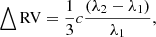
than what would correspond to the original resolution in the wavelength scale. The re-normalisation of the whole spectrum is carried out with the recursive formula:
where c is the speed of light in vacuum and sk are new pixel numbers in the RV scale (k = 1…M). The flipped spectrum in the RV scale, fj, is calculated for the line neighbourhood as:
and displayed on the screen in a different colour. The user can move the flipped spectrum on the computer screen interactively to achieve the best agreement between the original and flipped profile for the part of the line to be measured. The radial velocity RVmeas is derived from the shift △s in the s scale via
The advantage of this type of RV measurements over some automatic procedures is that the user clearly sees the quality of the profile and can avoid flaws or blends by telluric lines in the red parts of spectra. An automatic process of RV measurement for the Hα emission profile was compared to the manual one described here for the Be star γ Cas by Nemravová et al. (2012) with the result that the manual settings provided a lower scatter around the mean RV curve than the automatic one.
For the absorption lines, we made the settings on the line cores, while for the Hα emission, we measured the RV on the broad line wings. An illustration of this can be seen in Fig. C.2 of Harmanec et al. (2020). To obtain some estimate of the uncertainties involved, all such RV measurements were carried out independently by M. W. and P. H. and the average values of these were used.
All individual RVs collected from the literature and corrected for misprints are provided in Table 1; our RV measurements of the Hα, He I 6678 Å, Si II 6347 and 6371 Å doublet, and Fe II 6677 Å lines, along with their rms errors, are provided in Table 2. Spectrophotometric quantities measured on the Hα profiles collected from the literature and corrected for misprints are in Table 3 and our measurements of spectrophotometric quantities in the new electronic spectra are in Table 4. These four tables are published in their entirety only in the electronic form and are available at the CDS.
All RVs from the literature, edited and corrected for misprints.
All RVs with their rms errors (in km s−1) measured on electronic spectra at our disposal.
Spectrophotometry of Hα line from various published papers.
Spectrophotometric quantities measured on electronic spectra at our disposal for all five considered spectral lines.
3.2. Photometry
The star was rather systematically observed at Hvar over a number of observing seasons, first in the UBV, and later in the UBVR photometric systems. In addition, we tried to collect and homogenise all numerous photometric observations with known times of observation published by a number of investigations. The journal of these observations is in Table D.4 and details of the individual data sets can be found in Appendix B. All the individual photometric observations will be published in a separate study after we finish the final homogenisation and standardisation of our photometric archives.
4. Long-term changes
As we attempted to collect and homogenise most of the available spectral and photometric observations, we start our analysis with the description of long-term changes in various observed quantities and their mutual relation. This will provide a good starting point for any future quantitative modelling and the elimination of some possible models.
We first inspected the RV measurements on the electronic spectra at our disposal, plotted versus time in Fig. 1. One can see that all measured RVs undergo slow cyclic changes. Their amplitude differs from one line to another, being smallest for the He I 6678 absorption wings and largest for the Si II doublet. We also take note that there are phase shifts on the part of the RVs for individual measured features. To combine our RVs with the earlier ones, we chose the RV of the Hα absorption core, which could be measured for all our electronic spectra.
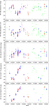 |
Fig. 1. Time plots of RVs (in km s−1) of individual measured features based on our new measurements. From top to bottom: Hα emission wing, Hα absorption core, He 6678 Å absorption wings, Fe II absorption core, and the mean Si II 6347&6371 Å. The RVs taken from the higher-resolution Elodie, Feros, and DAO are shown as blue circles, those from OND in red, those from the BeSS amateur spectra in green, and those from our re-measurements of the Trieste Hα spectra are shown as magenta circles. |
The time evolution of RV, V magnitude and B − V and U − B colour indices over the whole recorded history of observations is shown in Fig. 2. In Fig. B.1, we show additional photometric observations in several passbands different from the Johnson UBV photometry. They cover shorter time intervals.
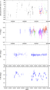 |
Fig. 2. Time evolution of absorption RV (mean RV from the literature, and the Hα core RV for all the new spectra at our disposal), the V magnitude, and B − V, and U − B colour indices over the whole time interval covered by available observations. In the RV plot, black dots show the RVs from the literature, blue circles are from our high signal-to-noise (S/N) spectra, red ones from OND spectra, and green ones from the BeSS spectra. In panels with photometry, blue dots denote calibrated UBV values, red the y magnitude of the Strömgren system, green the HIPPARCOSHp magnitudes transformed to Johnson V, magenta the ASAS3 V magnitude, and brown the KWS V magnitude. We note the shorter time interval covered by the observed colour changes. |
Figures 3 and 4 show the parallel time evolution of some spectrophotometric quantities measured in the Hα, Si II, Fe II 6677 Å, and He I 6678 Å line profiles. For the two last lines, which mutually blend with each other, it was only possible to measure their central intensities. Finally, Fig. 5 shows the variations in the U − B versus B − V diagram. Variations of another Be star V744 Her = 88 Her observed systematically at Hvar are also shown for comparison. We note the following:
-
The absorption-line RVs, V/R ratio of the strength of the violet and red peaks of the double Hα emission, star brightness, and U − B colour all undergo cyclic variations during the whole documented history, whereas the B − V index remains secularly quite stable and close to zero (compare Figs. 1–3). These variations are so regular that they look almost like a periodic phenomenon with a ’period’ of some 2400 days. We note, however, that the quantitative fits of individual cycles carried out in Sect. 5.2 show gradually varying length of consecutive cycles. While large parallel cyclic RV and V/R changes, which come and go, are known for many Be stars, the regular behavior observed for V923 Aql is rather rare. McLaughlin (1963) reported similar regularity for HD 20336 = BK Cam. Cyclic V/R and RV variations were observed between 1903–1937 and never since then. In the time interval between 1916–1931, they followed a regular 4.5 yr cycle, whereas outside that interval the cycles were longer. For 105 Tau = V1155 Tau, McLaughlin (1966) observed large parallel RV and V/R variations, with about a 10 yr ‘period’ over the time interval of 1930–1965.
-
The strength of the violet and red peaks of the Hα emission also varies cyclically and in the opposite manner (see Fig. 3). A notable fact is that the amplitude of these changes is larger for the V peak than for the R one in one cycle, while the opposite is true for the consecutive cycles. This indicates that the geometry of the envelope is dynamically evolving over time.
-
There is no systematic secular trend in either RV or brightness, perhaps with the exception of a slight recent brightening in the V band, as Fig. 2 shows. However, the Hα emission strength has been increasing over about 18 000 days covered by electronic spectra (cf. Fig. 3). A part of the increase has already been noted by Ruždjak (2008). It is best seen in the mean peak emission, measured as (IV + IR)/2. The same effect, but less clearly, is also seen in the EW of Hα. It is our experience that the errors in all, the relative flux, wavelength, choice of line range due to continuum placement for spectra with different S/N ratios, and the scatter due to variable strength of numerous telluric lines in the Hα region, contribute to the increased scatter of measured values of EW, making it less useful as the indicator of changes.
-
Variations in different photometric passbands show similar general trends but indicate that the amplitude of more rapid changes can depend on wavelength; see Figs. B.1 and B.2.
-
The spectral and photometric variations are clearly correlated, but in a complicated way, as documented by Figs. 1, 3, 4, and B.2. Cyclic RV variations of individual spectral features vary with mutual phase shifts and different amplitudes (growing from He to Si lines). The object becomes the brightest and bluest in U − B during the He and metallic-line RV minima and vice versa. The HαV/R ratio varies in phase with the metallic RVs. The central intensity Ic and the equivalent width EW of both Si II lines also vary cyclically, with the ∼2400 d cycle. The lines become weakest when the HαV/R ratio changes from V < R to V > R and when the U − B index is getting redder. The full width at half maximum (FWHM) of the Si II lines is largest, when their RV is decreasing but these variations show a great deal of scatter. The central intensity of Fe II 6677 Å line seems to follow the variations of Si II lines, while the Ic of the He I 6678 Å line does not exhibit any clear secular changes.
-
Variations in the U − B versus B − V diagram (Fig. 5) are typical for the inverse correlation between the emission strength and stellar brightness as defined by Harmanec (1983) and later modelled by Sigut & Patel (2013). Such correlation is observed for stars seen roughly equator-on.
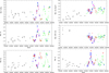 |
Fig. 3. Long-term spectral variations of the Hα line profile. From top to bottom: left panels show the ratio of the violet and red emission peak strength, normalised flux of the V peak, and normalised flux of the R peak. Right panels show the mean of the normalised fluxes in the V and R peak, equivalent width of the whole line, and central intensity of the core absorption. Data from the higher-resolution Elodie, Feros, and DAO are shown by blue circles, those from OND by the red circles, those from the BeSS amateur spectra by the green circles, those from the Trieste spectra re-reduced by us by magenta circles, and those from the literature by the black circles. |
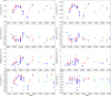 |
Fig. 4. Time evolution of the spectral changes of the Si II 6347 and 6371 Å, Fe II 6677 Å, and He I 6678 Å. Blue dots denote data from the higher-resolution Elodie, Feros, and DAO spectra, circles, the red ones those from OND spectra, and the green ones those from the BeSS amateur spectra. |
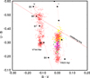 |
Fig. 5. U − B vs. B − V colour diagram showing the secular changes of V923 Aql. The object is reddened and moves along the main sequence. This is indicative of an inverse correlation between the brightness and emission-line strength. The data from different observatories are distinguished by different colours as follows: Hvar = red, SPM = blue, Tug = magenta, Canakkale = yellow, Haute Provence = black, Geneve = green, and Ondřejov = cyan. For comparison, the Hvar photometric observations of another systematically studied Be star V744 Her = 88 Her are also shown. They are less reddened but show a remarkably similar pattern of variations. |
In Fig. 6, we show selected Hα profiles over one whole 2400 d cycle and two DAO line profiles of metallic lines from the two extrema of the long-term V/R changes We note that the Si II line profiles for the spectrum with V > R are notably broader than those of the opposite extremum.
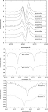 |
Fig. 6. Selected line profiles. Top: sequence of Hα profiles over one whole 2400 d cycle. Shifts of continua in ordinate are scaled in such a way to correspond to differences of individual spectra in RJD. Middle and bottom panels: comparison of two DAO Si II, and He I line profiles from the two consecutive extrema of the long-term V/R changes. |
5. Orbital and rapid changes
The scatter in the time plots for various quantities is certainly larger than the expected measuring errors, which is indicative of changes on shorter time scales. However, the simultaneous presence of rapid, orbital, and long-term changes makes the analysis rather complicated.
5.1. Rapid changes
Before addressing the orbital variations, we attempted to find a characteristic pattern of rapid variations occurring on a time scale of days. After a number of trials, we concluded that in spite of the large amount of photometric and spectral observations we are unable to identify a clear and unique pattern of such changes. The time distribution of the available data is insufficient with respect to this goal and only a systematic, uninterrupted series of future space observations may help to shed light on the nature of these changes.
In Fig. B.3, we show, for the purposes of illustration, the amplitude power spectra for three V magnitude data segments without any obvious secular trends. Their power spectra clearly differ from each other. In the upper panel of Fig. 7, individual Hvar 2020 V observations are plotted versus time, while the bottom plot shows a phase curve for the U magnitude (which has the largest amplitude) for the most prominent peak of the periodogram. We note that the period of 0 84417 is close to the originally suggested period of 0
 8518 (Lynds 1960). However, this periodicity is not seen in the first Hvar season. We also inspected several about 0
 2 long time series of DAO spectra. There might be some indication of rapid changes in the Si II line profiles, but once again, we were unable to document any clear pattern.
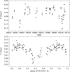 |
Fig. 7. Top: a time plot of the Hvar V photometry from the 2020 season. Rapid variations are quite obvious. Bottom: a phase plot of the Hvar U photometry for the 0 |

5.2. A new ephemeris of the orbital motion
We first extended the analysis that had previously been carried out by Koubský et al. (1989). We used all RVs listed in Table D.2, adopting the Hα absorption core RVs for all new spectra that we had already reduced. We removed their long-term changes (displayed in the top panel of Fig. 2) with the help of spline functions using the program HEC13, based on the Vondrák (1977) method3. For a comparison with Koubský et al. (1989), we used the same smoothing parameter ε = 1.0 ⋅ 10−15 as they did. The RV residuals were used as the input into program FOTEL, with which new circular orbital elements were derived. The results are in Table 5 and the phase plot is in the upper panel of Fig. 8.
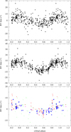 |
Fig. 8. Orbital RV curves after removal of the long-term cyclic changes. Top: residuals from a smoothing by Vondrák (1977) method, using the smoothing parameter ε = 1.0 s × 10−15. Middle: residuals from the local ‘triple-star’ solutions (see the text for details). Bottom: residuals for the RVs of the Hα emission wings also based on the ‘triple-star’ local solutions. Data from Feros, Elodie and DAO spectra are shown by blue circles, OND by red, Trieste by magenta, and BeSS by green circles. |
Several FOTEL orbital solutions for the RV residuals prewhitened for the long-term cyclic RV changes.
Next, we tried another approach. Using the subsets of RVs from reasonably well covered individual long cycles and the program FOTEL, we formally calculated ‘triple-star’ solutions, treating the ∼2000 d cycles as ‘an outer orbit’. This allowed us to obtain the residuals from the long cycles and combined them into one complete data set. As seen in the middle panel of Fig. 8, this resulted in a better-defined RV curve and a solution with lower mean rms error (cf. Table 5). As Table 6 shows, the length of individual cycles varied between about 1800 and 3000 days, as was already noted by Koubský et al. (1989).
Calculated duration of individual RV cycles as derived from the ‘triple-star’ solutions.
It is reassuring to note that the orbital elements obtained by the two different methods agree mutually within the limits of their errors. Thus, for the remainder of this study, we adopt the following linear ephemeris, based on the more accurate solution 2 of Table 5:

5.3. Final orbital elements and the properties of the binary
Harmanec (2003) showed that also seemingly photospheric absorption lines can be slightly filled by a weak emission coming from the rotating circumstellar envelope. Given the Roche-model geometry, it seems logical that more emission will come from the ‘nose’ of the Roche lobe, which is facing the secondary. This leads to a situation where, upon observing the Be component receding from us, it exhibits a maximum RV but since the violet wing of the line is more strongly filled by the emission, the measured RV of the apparently absorption line is actually more positive than what would correspond to the orbital RV at that orbital phase. An opposite effect is observed when the Be star is approaching to the observer. As a consequence, the amplitude of the RV curve of such an absorption line is higher than the true amplitude of the orbital motion. The effect is modelled and discussed in more detail in Appendix C. In contrast to it, the RV of the steep wings of the Hα emission, which is formed in the inner, more or less spherically symmetric parts of the Be disk, describes the true orbital velocity much better (see e.g. Harmanec et al. 2002; Ruždjak et al. 2009). This conclusion was nicely confirmed by Peters et al. (2013) who obtained the true RV curves of both components of V832 Cyg = 59 Cyg and found that the RV curve of the Be primary agrees with that derived from the Hα emission-wings RVs by Harmanec et al. (2002). The effect was found for quite a few binary Be stars.
We removed the cyclic RV changes of the Hα emission-wing RVs once again via local fits of a ‘triple-star’ solutions and then derived the final orbital solution 3 of Table 5, keeping the orbital period fixed at the value from ephemeris (6). The semi-amplitude of this solution is indeed smaller than those for solutions 1 and 2, based on absorption-line RVs.
Zorec et al. (2016) published a critical study of the distribution of rotational velocities of a group of Be stars including V923 Aql. They obtained observed radiative properties of the stars and their apparent v sin i values. They carefully analysed the effects of gravity darkening, macroturbulence, and other effects and then attempted to estimate corrected values that would correspond to non-rotating stars having the same mass as the studied objects. Their results for V923 Aql are summarised in Table 7. Using the corrected values, they also estimated the mass of V923 Aql m = 6.2 ± 0.3 M⊙ and inclination of the rotational axis i = 88° ±22°.
Observed and corrected radiative properties of V923 Aql derived by Zorec et al. (2016).
Using the corrected values above and interpolating them in a grid of non-rotating models of Schaller et al. (1992), we find that the radius of the star should be about 5.4 R⊙, which is in a broad agreement with the assumption that the photometric 0 84 period could be the rotational period of the star. However, the uncertainties of all parameters involved are too large to reach a firm conclusion.
Adopting the mass of 6.2 M⊙ for the Be primary and solution 3 of Table 5, we estimated the probable properties of the binary for several possible orbital inclinations. They are summarised in Table 8. It is clear that the semi-major axis is quite insensitive to the orbital inclination within the considered range of inclinations.
The HIPPARCOS (Perryman & ESA 1997) and Gaia (Gaia Collaboration 2016, 2018; Arenou et al. 2018) satellites measured the parallaxes of V923 Aql with following results:  (distance d from 237 to 391 pc), later revised by van Leeuwen (2007a,b) to
  (d = 230−269 pc), and
  (d = 234−327 pc), respectively. Adopting the Gaia DR2 value of the parallax, we estimate the angular projection of the semi-major axis of the V923 Aql binary to be
  . Horch et al. (2020) observed V923 Aql in 2015 as a part of their differential speckle survey and were unable to detect any wide companion at angular separations larger than 0
 2.
2.
6. Discussion
Okazaki (1991) was the first to suggest that the cyclic long-term variations of Be stars could be a consequence of a global one-armed oscillation in the Be star disk. Such an oscillation manifest itself as a density enhancement in an (essentially Keplerian) rotating disk, which gradually revolves in space, with a typical cycle length of several years. Oktariani & Okazaki (2009) investigated the properties of such oscillations for the binary Be stars. Telting et al. (1994) discussed the expected parameter correlations for that model for the objects seen roughly edge-on and predicted that for a prograde revolution of the density enhancement, the shell cores of the absorption lines should get deepest during the transition from V > R to V < R. Mennickent et al. (1997) attempted to interpret the observed light and spectral variations of several Be stars within the framework of that model. For V923 Aql, they had continuous uvby ESO photometry covering more than one long cycle and showing large cyclic variations in the u colour (see Fig. B.1 here). Using a limited set of HαV/R variations found by these authors from the literature, they tentatively suggested that the light minimum coincides with the cyclic transition from V > R to V < R, which indicates a prograde revolution of the one-arm oscillation.
The rich observational coverage of spectral, light, and colour variations that we collect here provides a very broad and detailed description that qualitatively supports the model of prograde one-arm oscillation. We recall that both the estimates of the disk inclination by Zorec et al. (2016) and our finding that V923 Aql shows an inverse correlation in the U − B versus B − V diagram indicate that we observe the disk more or less equator-on. Therefore, the shadowing effects of the density enhancement inside the disk are easily possible. However, the absence of detectable binary eclipses means that the inclination is not close to 90°. As Figs. 1–4, B.1, and B.2 show, the light minima, very pronounced in the ultraviolet passbands, indeed coincide with the phase, when V = R for the double Hα emission on the descending branch of the V/R curve. The measured central intensities for both the Hα core and metallic lines show that these shell lines indeed get deeper. However, they become strongest only some 500 days later than the photometric minima. This probably indicates that the revolving region of increased density is curved and lags behind the ‘root’ of one-arm oscillation wave during its revolution. This is why it produces the largest absorption against the stellar disk a bit later, as schematically shown in Fig. 9.
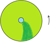 |
Fig. 9. Sketch of the model of the circumstellar disk around the Be component with one-armed density enhancement curved in space. |
A comparison of Figs. 3 and B.2 also shows that the Hα emission is strongest at the light minima and vice versa. We suspect that it can be only an apparent effect, a consequence of the fact that the observed continuum, to which the line is normalised, gets smaller during the light minima. Such an effect was documented for β Lyr by Ak et al. (2007). We note, however, that the secular increase of the emission strength over about 18 000 days has nothing to do with the one-armed oscillation and must be related to the still unknown mechanism of the formation and dispersal of Be envelopes.
7. Conclusion
In this work, we collect, homogenise, and analyse all the available spectral and photometric observations of the well-known emission-line Be star V923 Aql. We confirm the binary nature of the object and improve the accuracy of the value of its orbital period, adjusting it to: 214 716 ± 0
 033. We also provide the most complete description of its cyclic long-term changes. V923 Aql is a rather rare object, which has exhibited cyclic long-term changes over the whole recorded time interval of about 25000 days, during which it never lost the Balmer emission. By analysing the mutual relation of the variations in a number of observed variables, we were able to qualitatively confirm the tentative conclusion of Mennickent et al. (1997) stating that the long-term variations can be understood as variable shadowing of the stellar disk by the density enhancement produced by one-armed oscillation with a prograde revolution within the rotating Be-star disk.
We hope that the future comparison of similar studies for other well-observed Be stars will lead to a definition of the taxonomy of their variations, which is seemingly quite different for different objects, and to progress in improving our understanding of this intriguing class of hot stars. In a future study, we plan to apply a hydrodynamical model of the disk to a quantitative modelling of the observed changes.
The program was written by A. Harmanec and is available with the User manual at https://astro.troja.mff.cuni.cz/projects/respefo/
Program HEC13 with brief instructions on how to use it is available at https://astro.troja.mff.cuni.cz/ftp/hec/HEC13
The whole program suite with references to relevant studies, a detailed manual, examples of data, auxiliary data files, and results is available at http://astro.troja.mff.cuni.cz/ftp/hec/PHOT
Acknowledgments
We acknowledge the use of the program FOTEL written by P. Hadrava, and the program reSPEFO written by A. Harmanec. We thank P. Hadrava, A. Kawka, D. Korčáková, M. Kraus, J. Kubát, B. Kučerová, P. Neméth, M. Netolický, J. Polster, S. Vennes, and V. Votruba, who obtained a number of Ondřejov spectra used in this study. J.R. Percy kindly provided us with the digital archive of systematic UBV observations of bright Be stars secured by him and his collaborators. Our thanks also belong to G. Burki, who provided us with Geneva 7C observations of a number of Be stars, including V923 Aql, to H.F. Haupt, who provided us with their individual UBV observations secured at the OHP Chiron station, and to J. Gutiérrez-Soto, who provided us with the individual OSN uvby observations of V923 Aql. H. Maehara provided us with information about their KWS wide-field photometry and gave us the permission to use these data. Denis Gillet kindly provided us with copies of several OHP observing diaries, which allowed us to check the dates and times of exposures of the OHP spectra used by Denizman et al. (1994). During the corona lockdown in the spring of 2020, the staff of the Ondřejov Observatory Library put us into contact with E. Sulistialie from Bosscha Observatory who kindly sent us a copy of the Palmer et al. (1968) paper. This allowed us to check the times and RVs of V923 Aql published there. This work has made use of the BeSS database, operated at LESIA, Observatoire de Meudon, France: http://basebe.obspm.fr and we thank the following amateur observers, who contributed their spectra: P. Berardi, Ch. Buil, A. de Bruin, V. Desneoux, A. Favaro, O. Garde, T. Garrel, K. Graham, J. Guarro Fló, F. Houpert, P. Lailly, G. Martineau, J. Ribeiro, O. Thizy. We also thank to Jan Kára, who helped us to prepare the upper panel of Fig. C.1. Conctructive criticism and useful suggestions by an anonymous referee helped to improve the clarity of the paper and are greatly appreciated. P.H. and M.W. were supported by the Czech Science Foundation grant GA19-01995S. H.B. acknowledges financial support from Croatian Science Foundation under the project 6212 “Solar and Stellar Variability". D.R. acknowledges financial support from Croatian Science Foundation under the project 7549 “Millimeter and submillimeter observations of the solar chromosphere with ALMA". The following internet-based resources were consulted: the SIMBAD database and the VizieR service operated at CDS, Strasbourg, France; and the NASA’s Astrophysics Data System Bibliographic Services. This work has made use of data from the European Space Agency (ESA) mission Gaia (https://www.cosmos.esa.int/gaia), processed by the Gaia Data Processing and Analysis Consortium (DPAC; https://www.cosmos.esa.int/web/gaia/dpac/consortium). Funding for the DPAC has been provided by national institutions, in particular the institutions participating in the Gaia Multilateral Agreement.
References
- Aab, O. E., & Vojkhanskaya, N. F. 1977, Astrofizicheskie Issledovaniia Izvestiya Spetsial’noj Astrofizicheskoj Observatorii, 9, 22 [Google Scholar]
- Ak, H., Chadima, P., Harmanec, P., et al. 2007, A&A, 463, 233 [NASA ADS] [CrossRef] [EDP Sciences] [Google Scholar]
- Alduseva, V. Y., & Kolotilov, E. A. 1980, Astronomicheskij Tsirkulyar, 1111, 2 [Google Scholar]
- Arenou, F., Luri, X., Babusiaux, C., et al. 2018, A&A, 616, A17 [NASA ADS] [CrossRef] [EDP Sciences] [Google Scholar]
- Arias, M. L., Cidale, L. S., & Ringuelet, A. E. 2004, A&A, 417, 679 [EDP Sciences] [Google Scholar]
- Ballereau, D., Alvarez, M., Chauville, J., & Michel, R. 1987, RM&AC, 15, 29 [Google Scholar]
- Balona, L. A. 1995, MNRAS, 277, 1547 [NASA ADS] [Google Scholar]
- Bidelman, W. P. 1950, PASP [Google Scholar]
- Brož, M., Mourard, D., Budaj, J., et al. 2021, A&A, 645, A51 [EDP Sciences] [Google Scholar]
- Carciofi, A. C., Miroshnichenko, A. S., Kusakin, A. V., et al. 2006, ApJ, 652, 1617 [NASA ADS] [CrossRef] [Google Scholar]
- Carciofi, A. C., Okazaki, A. T., Le Bouquin, J. B., et al. 2009, A&A, 504, 915 [NASA ADS] [CrossRef] [EDP Sciences] [Google Scholar]
- Carciofi, A. C., Bjorkman, J. E., Otero, S. A., et al. 2012, ApJ, 744, L15 [NASA ADS] [CrossRef] [Google Scholar]
- Catanzaro, G. 2013, A&A, 550, A79 [NASA ADS] [CrossRef] [EDP Sciences] [Google Scholar]
- Denizman, L., Ak, T., Koktay, T., Saygac, T., & Kocer, D. 1994, Ap&SS, 222, 191 [NASA ADS] [CrossRef] [Google Scholar]
- Doazan, V., Sedmak, G., Barylak, M., & Rusconi, L. 1991, in A Be Star Atlas of Far UV and Optical High-resolution Spectra, ESA Spec. Pub., 1147 [Google Scholar]
- Fontaine, G., Villeneuve, B., Landstreet, J. D., & Taylor, R. H. 1982, ApJS, 49, 259 [NASA ADS] [CrossRef] [Google Scholar]
- Gaia Collaboration (Prusti, T., et al.) 2016, A&A, 595, A1 [NASA ADS] [CrossRef] [EDP Sciences] [Google Scholar]
- Gaia Collaboration (Brown, A. G. A., et al.) 2018, A&A, 616, A1 [NASA ADS] [CrossRef] [EDP Sciences] [Google Scholar]
- Ghoreyshi, M. R., Carciofi, A. C., Rímulo, L. R., et al. 2018, MNRAS, 479, 2214 [NASA ADS] [CrossRef] [Google Scholar]
- Gulliver, A. F. 1976, PhD thesis, University of Toronto, Canada [Google Scholar]
- Gutiérrez-Soto, J., Fabregat, J., Suso, J., et al. 2007, A&A, 476, 927 [NASA ADS] [CrossRef] [EDP Sciences] [Google Scholar]
- Hanuschik, R. W., Hummel, W., Sutorius, E., Dietle, O., & Thimm, G. 1996, A&AS, 116, 309 [NASA ADS] [CrossRef] [EDP Sciences] [Google Scholar]
- Harmanec, P. 1983, Hvar Obs. Bull., 7, 55 [NASA ADS] [Google Scholar]
- Harmanec, P. 1998, A&A, 335, 173 [NASA ADS] [Google Scholar]
- Harmanec, P. 2003, in New Directions for Close Binary Studies: The Royal Road to the Stars, eds. O. Demircan, & E. Budding, 221 [Google Scholar]
- Harmanec, P., & Božić, H. 2001, A&A, 369, 1140 [NASA ADS] [CrossRef] [EDP Sciences] [Google Scholar]
- Harmanec, P., & Horn, J. 1998, J. Astron. Data, 4, 5 [Google Scholar]
- Harmanec, P., Horn, J., & Juza, K. 1994, A&AS, 104, 121 [NASA ADS] [Google Scholar]
- Harmanec, P., Božić, H., Percy, J. R., et al. 2002, A&A, 387, 580 [NASA ADS] [CrossRef] [EDP Sciences] [Google Scholar]
- Harmanec, P., Lipták, J., Koubský, P., et al. 2020, A&A, 639, A32 [EDP Sciences] [Google Scholar]
- Harper, W. E. 1937, Pub. Dominion Astrophys. Obs. Victoria, 7, 1 [Google Scholar]
- Haubois, X., Carciofi, A. C., Rivinius, T., Okazaki, A. T., & Bjorkman, J. E. 2012, ApJ, 756, 156 [NASA ADS] [CrossRef] [Google Scholar]
- Haupt, H. F., & Schroll, A. 1974, A&AS, 15, 311 [NASA ADS] [Google Scholar]
- Horch, E. P., van Belle, G. T., Davidson, J. W., et al. 2020, AJ, 159, 233 [Google Scholar]
- Hubert, A. M., & Floquet, M. 1998, A&A, 335, 565 [NASA ADS] [Google Scholar]
- Jayasinghe, T., Stanek, K. Z., Kochanek, C. S., et al. 2019, MNRAS, 485, 961 [NASA ADS] [CrossRef] [Google Scholar]
- Kochanek, C. S., Shappee, B. J., Stanek, K. Z., et al. 2017, PASP, 129, 104502 [Google Scholar]
- Koubský, P., Gulliver, A. F., Harmanec, P., et al. 1989, Bull. Astron. Inst. Czechoslovakia, 40, 31 [Google Scholar]
- Kříž, S., & Harmanec, P. 1975, Bull. Astron. Inst. of Czechoslovakia, 26, 65 [Google Scholar]
- Kuschnig, R., Paunzen, E., & Weiss, W. W. 1994, IBVS, 4070, 1 [Google Scholar]
- Lee, U., Osaki, Y., & Saio, H. 1991, MNRAS, 250, 432 [NASA ADS] [CrossRef] [Google Scholar]
- Lynds, C. R. 1959, ApJ, 130, 577 [NASA ADS] [CrossRef] [Google Scholar]
- Lynds, C. R. 1960, ApJ, 131, 390 [NASA ADS] [CrossRef] [Google Scholar]
- Maehara, H. 2014, JAXA Research and Development Report JAXA-RR-13-010, 119 [Google Scholar]
- Manfroid, J., Sterken, C., Bruch, A., et al. 1991, A&AS, 87, 481 [NASA ADS] [Google Scholar]
- Manfroid, J., Sterken, C., Cunow, B., et al. 1995, A&AS, 109, 329 [NASA ADS] [Google Scholar]
- McLaughlin, D. B. 1963, ApJ, 137, 1085 [Google Scholar]
- McLaughlin, D. B. 1966, ApJ, 143, 285 [Google Scholar]
- Mennickent, R. E., Vogt, N., & Sterken, C. 1994, A&AS, 108, 237 [NASA ADS] [Google Scholar]
- Mennickent, R. E., Sterken, C., & Vogt, N. 1997, A&A, 326, 1167 [NASA ADS] [Google Scholar]
- Merrill, P. W. 1952, ApJ, 116, 501 [NASA ADS] [CrossRef] [Google Scholar]
- Neiner, C., de Batz, B., Cochard, F., et al. 2011, AJ, 142, 149 [Google Scholar]
- Nemravová, J., Harmanec, P., Koubský, P., et al. 2012, A&A, 537, A59 [NASA ADS] [CrossRef] [EDP Sciences] [Google Scholar]
- Okazaki, A. T. 1991, PASJ, 43, 75 [NASA ADS] [Google Scholar]
- Oktariani, F., & Okazaki, A. T. 2009, PASJ, 61, 57 [NASA ADS] [Google Scholar]
- Palmer, D. R., Walker, E. N., Jones, D. H. P., & Wallis, R. E. 1968, Roy. Greenwich Obs. Bull., 135, 385 [Google Scholar]
- Pavlovski, K., Harmanec, P., Božić, H., et al. 1997, A&AS, 125, 75 [NASA ADS] [CrossRef] [EDP Sciences] [Google Scholar]
- Percy, J. R., Coffin, B. L., Drukier, G. A., et al. 1988, PASP, 100, 1555 [NASA ADS] [CrossRef] [Google Scholar]
- Percy, J. R., Harlow, J., Hayhoe, K. A. W., et al. 1997, PASP, 109, 1215 [NASA ADS] [CrossRef] [Google Scholar]
- Percy, J. R., Hosick, J., Kincaide, H., & Pang, C. 2002, PASP, 114, 551 [NASA ADS] [CrossRef] [Google Scholar]
- Perryman, M. A. C., & ESA 1997, in The HIPPARCOS and TYCHO catalogues, (Noordwijk, Netherlands: ESA Publications Division), ESA SP Ser., 1200 the ESA Hipparcos Space Astrometry Mission [Google Scholar]
- Peters, G. J., Pewett, T. D., Gies, D. R., Touhami, Y. N., & Grundstrom, E. D. 2013, ApJ, 765, 2 [Google Scholar]
- Pojmanski, G. 2002, Acta Astron., 52, 397 [NASA ADS] [Google Scholar]
- Rachkovskaya, T. M. 1969, Izvestiya Ordena Trudovogo Krasnogo Znameni Krymskoj Astrofizicheskoj Observatorii, 39, 96 [Google Scholar]
- Ringuelet, A. E., & Sahade, J. 1981, PASP, 93, 594 [NASA ADS] [CrossRef] [Google Scholar]
- Ringuelet, A. E., Sahade, J., Rovira, M., Fontenla, J. M., & Kondo, Y. 1984, A&A, 131, 9 [NASA ADS] [Google Scholar]
- Rivinius, T., Carciofi, A. C., & Martayan, C. 2013, A&ARv, 21, 69 [Google Scholar]
- Ruždjak, D. 2008, Investigation of V/R variations in Be stars, Unpublished PhD Thesis, University of Zagreb, Faculty of Science, Department of Physics, 67 [Google Scholar]
- Ruždjak, D., Božić, H., Harmanec, P., et al. 2009, A&A, 506, 1319 [NASA ADS] [CrossRef] [EDP Sciences] [Google Scholar]
- Schaller, G., Schaerer, D., Meynet, G., & Maeder, A. 1992, A&AS, 96, 269 [Google Scholar]
- Shappee, B. J., Prieto, J. L., Grupe, D., et al. 2014, ApJ, 788, 48 [NASA ADS] [CrossRef] [Google Scholar]
- Sigut, T. A. A., & Patel, P. 2013, ApJ, 765, 41 [NASA ADS] [CrossRef] [Google Scholar]
- Sterken, C., Manfroid, J., Anton, K., et al. 1993, A&AS, 102, 79 [NASA ADS] [Google Scholar]
- Sterken, C., Manfroid, J., Beele, D., et al. 1995, A&AS, 113, 31 [NASA ADS] [Google Scholar]
- Szafraniec, R. 1948, Acta Astron., 4, 81 [Google Scholar]
- Telting, J. H., Heemskerk, M. H. M., Henrichs, H. F., & Savonije, G. J. 1994, A&A, 288, 558 [NASA ADS] [Google Scholar]
- van Leeuwen, F. 2007a, in Astrophysics and Space Science Library, ed. F. van Leeuwen, Astrophys. Space Sci. Lib., 350 [CrossRef] [Google Scholar]
- van Leeuwen, F. 2007b, A&A, 474, 653 [NASA ADS] [CrossRef] [EDP Sciences] [Google Scholar]
- Vondrák, J. 1977, Bull. Astron. Inst. Czechoslovakia, 28, 84 [Google Scholar]
- Zorec, J., Frémat, Y., Domiciano de Souza, A., et al. 2016, A&A, 595, A132 [NASA ADS] [CrossRef] [EDP Sciences] [Google Scholar]
Appendix A: Some notes on spectra from published papers
While collecting the RVs and spectrophotometric quantities from published papers, we noted - and if possible - corrected some misprints and other problems as detailed below.
-
The RVs published by Harper (1937) generally show such a smooth variation that we suspect there is a misprint for the spectrum taken on 1930 May 13 (RJD 26109.9755) and that the RV for this spectrum should read as −37.4 km s−1, and not the −57.4 km s−1 tabulated by the author.
-
Aab & Vojkhanskaya (1977) published RVs and Hα line profiles for a series of photographic spectra secured in 1974 at the Special Astrophysical Observatory (SAO). The list of these spectra is in Table 1 of their paper but the problem is that the dates of exposures quoted there are for one day earlier than the tabulated Julian dates, with the exception of the last spectrum, where the date and JD agree. Besides, the date of the last but one spectrum is not clear at all. They also tabulate phases, reportedly calculated for the photometric ephemeris given by Lynds (1960), but we were unable to reproduce these phases, no matter whether we considered the JDs from their table or JDs for one day earlier or later. They also measured RVs on 1965-1966 Crimean spectra studied earlier by Rachkovskaya (1969) but identified them only by the photometric phases, which we were unable to reproduce. Because of this, we only use mean RVs for mean JD of all those spectra for the description of the long-term RV changes.
-
Ringuelet & Sahade (1981) published an Hα profile from RJD 44450.7 (their Fig. 4), which shows a nearly symmetric double Hα emission with the peak intensity of about 1.5 of the continuum level. The same profile was again reproduced and measured by Arias et al. (2004) but with peak intensities of about 1.9! Arias et al. (2004) quote the (obviously) correct JD 2444450.740 for the first red CTIO spectrum in their Table 2 but give, probably by a mistake, JD 2444450.748 for this spectrum in their Table 3. This corresponds to the first blue CTIO spectrum. We adopted the value from their Table 2 for the determination of heliocentric RJD.
-
Denizman et al. (1994) tabulate JDs of the OHP spectra they used in their Tables II, IV, V, and VI. We noted some obvious problems. Denis Gillet from OHP kindly provided us with copies of original observing diaries and we spotted the following misprints in Table II: Correct JD of spectrum GA 7251 is 2446638.443 (not 2446683.443), for GA 7255 it is 2446640.486 (not 2446640.459; the correct value is in Table IV) and for GB 9208 the correct JD is 2446640.590 (not 2446640.912). As for other data sets, we used the mid-exposures from the OPH diaries to calculate heliocentric Julian dates for all these spectra.
-
Koubský et al. (1989) used only the first two spectra (out of three) from the paper by Ballereau et al. (1987). There is also a misprint in the quotation of the first page of paper by Palmer et al. (1968): 71 is given instead of the correct 385.
-
The BeSS database contains one low-resolution (R = 6000) red spectrum obtained by French amateur astronomer Eric Barbotin. The R peak of the Hα profile has an anomalously high intensity and differs dramatically from some other BeSS spectra taken only a few days apart. Mr. Barbotin informed us upon our inquiry that he is no longer active in the field of stellar spectroscopy and does not have the software needed to re-reduce the spectrum. As a precaution, we do not use any quantities measured on his spectrum (file M of Table D.1).
Appendix B: Details on the photometric data reductions and some additional data plots
Since we used photometry from various sources and photometric systems, both all-sky and differential, relative to several different comparison stars, we attempted to arrive at some homogenisation and standardisation. Observations from several observatories were reduced and transformed to the standard UBV system with the help of the reduction program HEC22, which uses non-linear seasonal transformation formulæ and models changes of the atmospheric extinction in the course of observing nights. See Harmanec et al. (1994) and Harmanec & Horn (1998) for the observational strategy and data reduction4.
Special efforts were made to derive improved all-sky values for the comparison stars used by observers at different observatories, employing carefully standardised UBV observations secured at Hvar (station 01) over several decades of systematic observations. The adopted values are collected in Table B.1, together with the number of all-sky observations and the rms errors of one observation. They were added to the respective magnitude differences for all available differential observations from all observing stations to obtain directly comparable standard UBV magnitudes. To demonstrate the internal consistency of all-sky data from other observing stations, whose data were reduced with the program HEC22, we also show there the UBV values of observed comparison stars from these stations.
Mean all-sky UBV values for all comparison stars used.
Below, we provide some details of the individual data sets and their reductions.
-
Station 01 – Hvar. These differential observations have been secured by a number of Croatian and Czech observers. Initially, 35 Aql = HD 183324 was used as the principal comparison. However, after Kuschnig et al. (1994) reported its microvariability on the 0m.01 level and the star obtained a variable-star name V1431 Aql, we used HR 7397 = HD 183227 as a new comparison. In several cases, the check star HR 7438 = HD 184663 was used as the comparison. The check star was usually observed as frequently as the variable. All observations were transformed into the standard UBV system via non-linear transformation formulæ with the program HEC22.
-
Station 12 – ESO La Silla. These differential Strömgren uvby observations were obtained and transformed into the standard system in the course of the ESO long-term monitoring campaign (Manfroid et al. 1991, 1995; Sterken et al. 1993, 1995). Comparisons V1431 Aql and HR 7397 were observed along with V923 Aql.
-
Station 20 – Toronto. These B and V observations were secured relative to HR 7397 by Percy et al. (1988, 1997) and transformed into the standard system via linear transformation formulæ by the authors. We just added the Hvar mean all-sky values of HR 7397 to their magnitude differences.
-
Station 30 – San Pedro Mártir. These UBV observations were obtained by M.W. and reduced to the standard system with the program HEC22 in a similar way as the Hvar data.
-
Station 37 – Jungfraujoch. These all-sky seven-colour (7-C) observations were secured in the Geneva photometric system using the P3 photometer mounted on the 0.76 m reflector. They were transformed into the UBV using the transformation formulae given by Harmanec & Božić (2001).
-
Station 44 – Mount Palomar. These observations were secured by Lynds (1959) with a 0.51 m reflector and a photometer with EMI 6094 tube though yellow Corning 3384 filter, relative to HR 7438. Inspecting the magnitude differences yellow - Johnson V filter for a number of microvariables observed by Lynds (1959), we found that the observations are very close to the Johnson V filter. We thus only added the Hvar V magnitude of HR 7438 to the Lynds (1960) magnitude differences V923 Aql – HR 7438.
-
Station 61 – HIPPARCOS. These all-sky observations were reduced to the standard V magnitude via the transformation formulæ derived by Harmanec (1998) to verify that no secular light changes in the system were observed.
-
Station 66 – Tubitak. These differential UBV observations were obtained by one of us (H. A.) and transformed to the standard system with the help of the program HEC22.
-
Station 89 – Canakkale. There differential UBV observations were also obtained by two of us (H. Bakış and V. Bakış) and reduced with the program HEC22.
-
Station 93 – ASAS3 V photometry. We extracted these all-sky observations from the ASAS3 public archive (Pojmanski 2002), using the data for diaphragm 1, having, on average, the lowest rms errors. We omitted all observations of grade D and observations having rms errors larger than 0m.04. We also omitted a strongly deviating observation at HJD 2452662.6863.
-
Station 114 – ASAS-SN network. These V and g band photometries were downloaded from the ASAS-SN database and cleaned for some deviating data points. We note that the V band photometry is for about 0m.5 fainter than the usual Johnson V.
-
Station 117 – KWS V and Ic photometry. We extracted these CCD photometric observations (Maehara 2014) from http://kws.cetus-net.org/~maehara/VSdata.py database. It is aperture photometry with fixed aperture radius. The flux zero-point calibration was carried out by the author, who used stars of magnitudes 5–9 having B − V < 1.5 and a scatter smaller than 0m.03 in the Hp magnitude. All the V and Ic were published as instrumental magnitudes. The preliminary transformation formulae to the standard magnitudes, derived by the author (Maehara, priv. comm.), are:
and
where B − V and Ic are the standard values from the HIPPARCOS catalogue. Since B − V ∼ 0 for V923 Aql, we adopted the instrumental V magnitudes for the standard ones. When using these observations, we omitted a few deviating data points.
-
Station 118 – Sierra Nevada (OSN). These differential uvby observations were obtained by Gutiérrez-Soto et al. (2007) and kindly provided by Juan Gutiérrez Soto as magnitude differences relative to the comparison star.


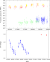 |
Fig. B.1. Time evolution of various photometric observations in different passbands. Top: green dots denote the ASAS-SN V magnitude (which is for some 0m.5 fainter than the usual Johnson V magnitude, blue dots denote the ASAS-SN g filter observations, red dots denote the KWS Cousins’ Ic observations, and yellow dots denote Hvar Johnson R observations. Bottom: stromgren u − b index from ESO observations (blue) and from Sierra Nevada differential photometry (red). The data generally confirm the long-term trends seen in the UBV photometry (cf. Fig. 2), but with different amplitude and scatter. |
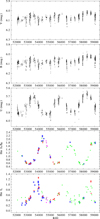 |
Fig. B.2. Time evolution of calibrated UBV photometry from stations 1, 20, and 30 (black), and Hα spectrophotometry (V/R and Ic) over a limited time interval RJD 51500 to 59500, which is covered by electronic spectra. Data from the higher-resolution Elodie, Feros, and DAO are shown by blue circles, those from OND by the red circles, those from the BeSS amateur spectra by the green circles, those from the Trieste spectra re-reduced by us by magenta circles. |
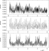 |
Fig. B.3. Amplitude periodograms for three V magnitude data subsets over the range from 0 |


Appendix C: An explanation for the origin of incorrect semi-amplitudes of seemingly photopheric lines of Be stars in binary systems
As shown in the upper panel of Fig. C.1, it is probable that as the Be disk fills a large part of the volume given by the dimensions of the critical Roche lobe around the Be-star primary and there will be more emission power in the part of the envelope facing the secondary. Since the disk rotates, this implies that when the Be star is receding from the observer and has a maximum RV, also the phase-locked V/R changes will attain their maximum. If, in addition, the seemingly photospheric absorption line of the Be star is actually partly blended with a weak emission contribution from the disk, the phase-locked V/R changes can affect the measured position of such a line.
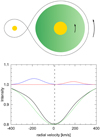 |
Fig. C.1. Illustration of the systematic distortion of seemingly photospheric absorption lines of Be stars in binaries due to unnoticed weak emission from the envelope with phase-locked V/R changes. Top: sketch of the Be-star circumstellar disk located inside the Roche lobe of a binary system (with a mass ratio of 0.1 in this example). Bottom: plot shows a superposition of the true rotationally broadened photospheric line profile (green) with a weak double-peak emission having V/R > 1 (simulated by the blue and red Gaussians). The resulting (black) profile has a more positive RV than the original profile. This situation corresponds to an observation at the elongation with the Be component receding from us. Just the opposite happens at the other elongation. |
We attempted to model the situation replacing the true spectral lines by the Gaussian profiles simulating the absorption and double emission profile. The result of their superposition is shown in the bottom panel of Fig. C.1 for the elongation with the Be star receding from us. It can be seen that this leads to a small but significant shift of the RV measured on the resulting (and still apparent) absorption line. In the chosen example, the shift amounts to +10 km s−1 in the elongation when the V/R is at maximum and the Be star is receding from us. In the opposite elongation, it is −10 km s−1, of course. As a consequence, the RV curve measured on such a seemingly photospheric absorption line has a larger amplitude than what would correspond to the true amplitude of the orbital RV curve of the Be star itself.
Appendix D: Journals of spectroscopic and photometric observations of V923 Aql
Journal of spectroscopic observations of V923 Aql.
Journal of all RV data sets.
Journal of available records of the Hα profile.
Journal of available photometry.
All Tables
All RVs with their rms errors (in km s−1) measured on electronic spectra at our disposal.
Spectrophotometric quantities measured on electronic spectra at our disposal for all five considered spectral lines.
Several FOTEL orbital solutions for the RV residuals prewhitened for the long-term cyclic RV changes.
Calculated duration of individual RV cycles as derived from the ‘triple-star’ solutions.
Observed and corrected radiative properties of V923 Aql derived by Zorec et al. (2016).
All Figures
|
Fig. 1. Time plots of RVs (in km s−1) of individual measured features based on our new measurements. From top to bottom: Hα emission wing, Hα absorption core, He 6678 Å absorption wings, Fe II absorption core, and the mean Si II 6347&6371 Å. The RVs taken from the higher-resolution Elodie, Feros, and DAO are shown as blue circles, those from OND in red, those from the BeSS amateur spectra in green, and those from our re-measurements of the Trieste Hα spectra are shown as magenta circles. |
| In the text | |
|
Fig. 2. Time evolution of absorption RV (mean RV from the literature, and the Hα core RV for all the new spectra at our disposal), the V magnitude, and B − V, and U − B colour indices over the whole time interval covered by available observations. In the RV plot, black dots show the RVs from the literature, blue circles are from our high signal-to-noise (S/N) spectra, red ones from OND spectra, and green ones from the BeSS spectra. In panels with photometry, blue dots denote calibrated UBV values, red the y magnitude of the Strömgren system, green the HIPPARCOSHp magnitudes transformed to Johnson V, magenta the ASAS3 V magnitude, and brown the KWS V magnitude. We note the shorter time interval covered by the observed colour changes. |
| In the text | |
|
Fig. 3. Long-term spectral variations of the Hα line profile. From top to bottom: left panels show the ratio of the violet and red emission peak strength, normalised flux of the V peak, and normalised flux of the R peak. Right panels show the mean of the normalised fluxes in the V and R peak, equivalent width of the whole line, and central intensity of the core absorption. Data from the higher-resolution Elodie, Feros, and DAO are shown by blue circles, those from OND by the red circles, those from the BeSS amateur spectra by the green circles, those from the Trieste spectra re-reduced by us by magenta circles, and those from the literature by the black circles. |
| In the text | |
|
Fig. 4. Time evolution of the spectral changes of the Si II 6347 and 6371 Å, Fe II 6677 Å, and He I 6678 Å. Blue dots denote data from the higher-resolution Elodie, Feros, and DAO spectra, circles, the red ones those from OND spectra, and the green ones those from the BeSS amateur spectra. |
| In the text | |
|
Fig. 5. U − B vs. B − V colour diagram showing the secular changes of V923 Aql. The object is reddened and moves along the main sequence. This is indicative of an inverse correlation between the brightness and emission-line strength. The data from different observatories are distinguished by different colours as follows: Hvar = red, SPM = blue, Tug = magenta, Canakkale = yellow, Haute Provence = black, Geneve = green, and Ondřejov = cyan. For comparison, the Hvar photometric observations of another systematically studied Be star V744 Her = 88 Her are also shown. They are less reddened but show a remarkably similar pattern of variations. |
| In the text | |
|
Fig. 6. Selected line profiles. Top: sequence of Hα profiles over one whole 2400 d cycle. Shifts of continua in ordinate are scaled in such a way to correspond to differences of individual spectra in RJD. Middle and bottom panels: comparison of two DAO Si II, and He I line profiles from the two consecutive extrema of the long-term V/R changes. |
| In the text | |
|
Fig. 7. Top: a time plot of the Hvar V photometry from the 2020 season. Rapid variations are quite obvious. Bottom: a phase plot of the Hvar U photometry for the 0 |
| In the text | |
|
Fig. 8. Orbital RV curves after removal of the long-term cyclic changes. Top: residuals from a smoothing by Vondrák (1977) method, using the smoothing parameter ε = 1.0 s × 10−15. Middle: residuals from the local ‘triple-star’ solutions (see the text for details). Bottom: residuals for the RVs of the Hα emission wings also based on the ‘triple-star’ local solutions. Data from Feros, Elodie and DAO spectra are shown by blue circles, OND by red, Trieste by magenta, and BeSS by green circles. |
| In the text | |
|
Fig. 9. Sketch of the model of the circumstellar disk around the Be component with one-armed density enhancement curved in space. |
| In the text | |
|
Fig. B.1. Time evolution of various photometric observations in different passbands. Top: green dots denote the ASAS-SN V magnitude (which is for some 0m.5 fainter than the usual Johnson V magnitude, blue dots denote the ASAS-SN g filter observations, red dots denote the KWS Cousins’ Ic observations, and yellow dots denote Hvar Johnson R observations. Bottom: stromgren u − b index from ESO observations (blue) and from Sierra Nevada differential photometry (red). The data generally confirm the long-term trends seen in the UBV photometry (cf. Fig. 2), but with different amplitude and scatter. |
| In the text | |
|
Fig. B.2. Time evolution of calibrated UBV photometry from stations 1, 20, and 30 (black), and Hα spectrophotometry (V/R and Ic) over a limited time interval RJD 51500 to 59500, which is covered by electronic spectra. Data from the higher-resolution Elodie, Feros, and DAO are shown by blue circles, those from OND by the red circles, those from the BeSS amateur spectra by the green circles, those from the Trieste spectra re-reduced by us by magenta circles. |
| In the text | |
|
Fig. B.3. Amplitude periodograms for three V magnitude data subsets over the range from 0 |
| In the text | |
|
Fig. C.1. Illustration of the systematic distortion of seemingly photospheric absorption lines of Be stars in binaries due to unnoticed weak emission from the envelope with phase-locked V/R changes. Top: sketch of the Be-star circumstellar disk located inside the Roche lobe of a binary system (with a mass ratio of 0.1 in this example). Bottom: plot shows a superposition of the true rotationally broadened photospheric line profile (green) with a weak double-peak emission having V/R > 1 (simulated by the blue and red Gaussians). The resulting (black) profile has a more positive RV than the original profile. This situation corresponds to an observation at the elongation with the Be component receding from us. Just the opposite happens at the other elongation. |
| In the text | |
Current usage metrics show cumulative count of Article Views (full-text article views including HTML views, PDF and ePub downloads, according to the available data) and Abstracts Views on Vision4Press platform.
Data correspond to usage on the plateform after 2015. The current usage metrics is available 48-96 hours after online publication and is updated daily on week days.
Initial download of the metrics may take a while.