| Issue |
A&A
Volume 646, February 2021
|
|
|---|---|---|
| Article Number | A8 | |
| Number of page(s) | 13 | |
| Section | Cosmology (including clusters of galaxies) | |
| DOI | https://doi.org/10.1051/0004-6361/202038807 | |
| Published online | 29 January 2021 | |
Clustering of CODEX clusters
1
Department of Physics, University of Helsinki, Gustaf Hällströmin katu 2 A, Helsinki, Finland
e-mail: This email address is being protected from spambots. You need JavaScript enabled to view it.
2
Helsinki Institute of Physics, University of Helsinki, Gustaf Hällströmin katu 2, Helsinki, Finland
3
Max-Planck institute for Extraterrestrial physics, Giessebachstr, Garching 85748, Germany
4
Kavli Institute for Particle Astrophysics & Cosmology, Stanford University, PO Box 2450, Stanford, CA 94305, USA
5
SLAC National Accelerator Laboratory, Menlo Park, CA 94025, USA
6
IRAP, Université de Toulouse, CNRS, UPS, CNES, Toulouse, France
7
Astrophyics Research Institute, Liverpool John Moores University, IC2, Liverpool Science Park, 146 Brownlow Hill, Liverpool L3 5RF, UK
8
Instituto de Astrofísica, Pontificia Universidad Católica de Chile, Av. Vicuna Mackenna 4860, 782-0436 Macul, Santiago, Chile
Received:
1
July
2020
Accepted:
17
November
2020
Abstract
Context. The clustering of galaxy clusters links the spatial nonuniformity of dark matter halos to the growth of the primordial spectrum of perturbations. The amplitude of the clustering signal is widely used to estimate the halo mass of astrophysical objects. The advent of cluster mass calibrations enables using clustering in cosmological studies.
Aims. We analyze the autocorrelation function of a large contiguous sample of galaxy clusters, the Constrain Dark Energy with X-ray (CODEX) sample, in which we take particular care of cluster definition. These clusters were X-ray selected using the ROentgen SATellite All-Sky Survey and then identified as galaxy clusters using the code redMaPPer run on the photometry of the Sloan Digital Sky Survey. We develop methods for precisely accounting for the sample selection effects on the clustering and demonstrate their robustness using numerical simulations.
Methods. Using the clean CODEX sample, which was obtained by applying a redshift-dependent richness selection, we computed the two-point autocorrelation function of galaxy clusters in the 0.1 < z < 0.3 and 0.3 < z < 0.5 redshift bins. We compared the bias in the measured correlation function with values obtained in numerical simulations using a similar cluster mass range.
Results. By fitting a power law, we measured a correlation length r0 = 18.7 ± 1.1 and slope γ = 1.98 ± 0.14 for the correlation function in the full redshift range. By fixing the other cosmological parameters to their nine-year Wilkinson Microwave Anisotropy Probe values, we reproduced the observed shape of the correlation function under the following cosmological conditions: Ωm0 = 0.22−0.03+0.04 and S8 = σ8(Ωm0/0.3)0.5 = 0.85−0.08+0.10 with estimated additional systematic errors of σΩm0 = 0.02 and σS8 = 0.20. We illustrate the complementarity of clustering constraints by combining them with CODEX cosmological constraints based on the X-ray luminosity function, deriving Ωm0 = 0.25 ± 0.01 and σ8 = 0.81−0.02+0.01 with an estimated additional systematic error of σΩm0 = 0.07 and σσ8 = 0.04. The mass calibration and statistical quality of the mass tracers are the dominant source of uncertainty.
Key words: large-scale structure of Universe / cosmology: observations / galaxies: clusters: general
© ESO 2021
1. Introduction
Galaxy clusters are the largest gravitationally bound objects in the Universe. A common assumption is that they completely and uniquely trace the population of the high-mass dark matter halos. Thus galaxy clusters form a powerful probe for the large-scale structure of the Universe. This power is further enhanced by the fact that several of the galaxy cluster properties, such as the abundance as a function of total mass and spatial clustering, can be predicted based on a cosmological model. A particularly important aspect of the clustering of clusters is that they are biased tracers of the underlying matter distribution, meaning that their clustering amplitude is higher than that of the full distribution of matter. Moreover, the amount of enhancement grows with increasing cluster masses. By studying the relationship between cluster masses and bias, we can gain further insights into the cosmology (see, e.g., Mo & White 1996; Sheth & Tormen 1999)
Because the clustering amplitude of dark matter halos of a given mass is sensitive to the underlying cosmology, the application of the clustering theory to galaxy clusters is theoretically highly motivated. Moreover, galaxy clusters exhibit scaling relations between their baryonic properties and the total mass of their hosting halos. These properties include the cluster X-ray luminosity and richness (i.e., the number of galaxies belonging to the cluster). Using these observable quantities as mass proxies on the one hand and the connection between cluster masses and their bias on the other, we can make inference on the cosmological model. Most attempts to follow this route have resulted in cosmological parameters that disagree with the constraints obtained using the number counts of the same sample (Schuecker et al. 2002), however, or lead to strongly disagreeing scaling relations (Jimeno et al. 2017). Remarkably, Allevato et al. (2012) obtained a precise agreement between the modeling of the clustering based on the weak-lensing mass calibration and the measured clustering amplitudes of galaxy groups by taking the definition of the object and the effects of sample variance into account.
The goal of this paper is to measure the clustering of galaxy clusters detected in the galaxy cluster survey called Constrain Dark Energy with X-ray (CODEX; Finoguenov et al. 2020) by computing their auto two-point correlation function. A brief description of the CODEX catalog is given in Sect. 2. Furthermore, we aim at predicting the excess clustering, quantified by the bias factor, based on the cluster masses and a cosmological prediction for the total matter distribution. The details of this procedure are presented in Sect. 3, which is a continuation of the developments presented in Allevato et al. (2011, 2012). In Sect. 4 we apply this pipeline to a simulated dark matter halo catalog to ensure that the predicted and measured clustering amplitudes match. In Sect. 5 we present the clustering measurements for the CODEX cluster catalog. Finally, in Sect. 6 we use the measured and predicted clustering amplitudes to constrain two parameters within the spatially flat ΛCDM cosmology: the matter density parameter Ωm0, and the power spectrum normalization σ8. Similar analyses have been performed, for example, by Marulli et al. (2018) using data from another X-ray selected survey, the XXL survey (Pierre et al. 2016), and by Annalisa et al. (2013) for a cluster sample selected using the maxBCG red-sequence method from Sloan Digital Sky Survey (SDSS) photometric data (Koester et al. 2007). A key improvement with the CODEX catalog compared to the first analysis is the significantly larger sample size (1892 clusters in our analysis here compared to 187 clusters), and compared to the second analysis, we gain an improvement through the X-ray selection.
2. CODEX galaxy cluster survey and its modeling
The CODEX galaxy cluster survey is constructed by performing the detection of faint X-ray sources in the ROentgen SATellite (ROSAT) All-Sky Survey (RASS) and a subsequent identification of those sources using the redMaPPer algorithm (Rykoff et al. 2014) applied to the SDSS photometry inside the 10 000 square degree area of the Baryon Oscillation Spectroscopic Survey (BOSS) footprint. A detailed description of the survey and the catalog is presented in Finoguenov et al. (2020). Spectroscopic identification of the sample has been a target of the SPectroscopic IDentification of eROSITA Sources (SPIDERS) program of SDSS-IV, with first results presented in Clerc et al. (2016, 2020). These first results confirmed the high quality of the redMaPPer redshifts and the virialized nature of CODEX clusters.
To perform the clustering analysis, we selected the clean CODEX catalog by applying a richness cut
 (1)
(1)
where z denotes the redshift of the cluster and λ ≡ ln(SDSS Richness) (defined at the optical peak, with a detailed description provided in Rykoff et al. 2014). We describe the effect of this cleaning as a PRASS(I|λ, z) term in the modeling. Because we use multivariate log-normal distributions throughout this paper, we conveniently define the quantities rc ≡ ln(Rc) (core radius of the X-ray surface brightness), l ≡ ln(Lx) (rest-frame X-ray luminosity in the 0.1–2.4 keV band), μ ≡ ln(M200c) (total mass measured within the overdensity of 200 with respect to the critical density). In addition to the redshift-dependent richness cut, we also discarded all clusters with richness below 25. The lowest and highest redshifts in the cleaned catalog are 0.047 and 0.682, respectively, but we restrict our analysis to the range 0.1 < z < 0.5. After the richness cut, 1892 clusters lie within this redshift range.
We applied the BOSS stellar mask to remove the areas affecting optical cluster detection. We considered that the optical completeness of the CODEX catalog above the applied richness cut does not to vary over the BOSS area and modeled it using
 (2)
(2)
which was obtained using the tabulations of Rykoff et al. (2014). We used an error function with the mean of λ50%(z) and a σ = 0.2, which reproduces the 75% and 90% quantiles of the distribution tabulated in Rykoff et al. (2014). We used the probability of the optical detection of the cluster in SDSS data as
 (3)
(3)
We verified the lack of sensitivity toward variations in the photometric depths using an agreement in the clustering signal between Northern and Southern Galactic Cap areas and using the tests for the presence of artificial correlation due to the bright stars.
The RASS survey has large spatial inhomogeneities in its coverage; the limiting flux changes by a factor of 10. To properly account for the variation in the spatial distribution caused by it, we generated a random catalog in which the number of objects was six times higher than in the real catalog. We divided the survey area into 100 zones of equal sensitivity S, with a 12% step in flux sensitivity between the subsequent zones. We denote the sky area of these zones as ΔΩS. We computed the probability of cluster detection
 (4)
(4)
where η denotes X-ray count (superscript “true” stands for predicted and “ob” for observed),  , and all the probabilities are described in detail in Finoguenov et al. (2020). This modeling accounts for the effect of the X-ray shape (rc, β) of the clusters and for the RASS sensitivity on the cluster selection, and predicts changes in the distribution of X-ray shapes based on the measured covariance of cluster properties (Cavaliere & Fusco-Femiano 1976; Mulroy et al. 2019; Farahi et al. 2019; Käfer et al. 2019). In this way, we accounted for the effect of the anticorrelation between the scatter of the X-ray luminosity and the optical richness and of the anticorrelation of the core radii of galaxy clusters and their scatter in luminosity. Our simulations reproduce the correct mix of shapes, luminosities, and richnesses of galaxy clusters. They were then used for the cluster detection modeling in all areas of the survey.
We estimated the expected number of clusters in each bin of redshift as
 (5)
(5)
where
 (6)
(6)
Figure 2 shows a correspondence of the slope of the dn/dz distribution of the real clusters and the random catalog. They agree well.
 |
Fig. 1. Sky footprint of the subset of the CODEX catalog used to compute the two-point correlation function. Orange points show the clusters, and blue points show the random points. |
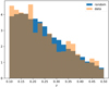 |
Fig. 2. Redshift distribution (dn/dz) of the subset of the CODEX catalog used to compute the two-point correlation function along with the corresponding random catalog. The area of the two histograms is normalized to 1. |
3. Analysis methods
Our clustering analysis consists of first estimating the clustering of the clusters by computing their two-point correlation function; next, computing the expected bias of the sample from the cluster masses and redshifts; then, computing a prediction for the clustering signal by scaling a prediction for dark matter two-point correlation by the square of the predicted bias; and finally, comparison between the measured and predicted signals.
We used the widely adopted Landy-Szalay estimator (Landy & Szalay 1993) to estimate the two-point correlation function from our cluster sample. The estimator was constructed from pairs within the cluster catalog (DD), pairs within the random catalog (RR), and pairs between the two (DR):
 (7)
(7)
where r is a vector encoding arbitrary separation bins, nD is the total number of clusters, and nR is the total number of random points. The simplest way to bin number counts is by their three-dimensional distance. This estimate is distorted by changes in cluster positions along the line-of- sight direction due to redshift caused by their peculiar velocities, however. These redshift space distortions can be minimized by estimating the so-called projected two-point correlation function (Davis & Peebles 1983). The projected two-point correlation function is the line-of-sight integral of two-point correlation function that has been binned in distance of the points along directions parallel and perpendicular to the line-of-sight direction:
 (8)
(8)
The upper limit of the integral is selected in a way that increasing it would only increase noise and not the signal.
We estimated the covariance matrix of the two-point correlation function using the jackknife method: we split the sample into M subsections of the sky and computed a set of two-point correlation functions by excluding one subsection at a time. The covariance matrix element Cij was then computed as
![Mathematical equation: $$ \begin{aligned} C_{ij} = \frac{M-1}{M}\sum _{k=1}^M [ \xi _k(r_i) - \langle \xi _k(r_i)\rangle ] [ \xi _k(r_j) - \langle \xi _k(r_j)\rangle ], \end{aligned} $$](/articles/aa/full_html/2021/02/aa38807-20/aa38807-20-eq13.gif) (9)
(9)
where ⟨ξk(rj)⟩ is the mean over M subsections. All the error bars we show for the two-point correlation function estimates are then the square root of the diagonal of this matrix,  .
.
As discussed in the introduction, galaxy clusters are biased tracers of the total matter distribution, and their clustering bias is connected to dark matter masses of their host halos. The goal of our analysis is to compare mass-based cluster bias predictions to the actual bias measured from the two-point correlation function estimate. Thus a key ingredient in our analysis is the relation between cluster masses and their biases. It is possible to predict the clustering bias based on the mass function n(M), that is, the number density of halos of a given mass, using the so-called peak background split (see, e.g., Mo & White 1996; Sheth & Tormen 1999). In this approach it is customary to consider masses in terms of the variance of the linear matter power spectrum P(k, z),
 (10)
(10)
where W(k, M) is the Fourier transform of a top-hat window function at  that encloses mass M. Here
  is the mean matter density in the Universe. For cleaner notation, we write in in Eqs. (11)–(14) σ instead of σ(M, z). Now the halo mass function can be expressed as
 (11)
(11)
where f(σ) is so-called multiplicity function. It is simply the fraction of mass contained in halos in a unit range of dlnσ. Using the ellipsoidal collapse model, Sheth et al. (2001) arrived at a parameterized multiplicity function,
![Mathematical equation: $$ \begin{aligned} \begin{array}{@ll}&f_{\mathrm{ST} }(\sigma ; A, a, p) = A \sqrt{\frac{2}{\pi }}\left[1 + \left(\frac{\sigma ^2}{a^2\delta _c^2}\right)^{p}\right] \\&\qquad \qquad \qquad \left(\frac{\sqrt{a}\delta _c}{\sigma }\right)\exp \left[-\frac{a}{2}\frac{\delta _c^2}{\sigma ^2} \right], \end{array} \end{aligned} $$](/articles/aa/full_html/2021/02/aa38807-20/aa38807-20-eq19.gif) (12)
(12)
where δc = 1.686 is the critical density for halo collapse. To improve the compatibility with N-body simulations, Bhattacharya et al. (2011) introduced an additional ad hoc parameter q, which is a function of redshift, and changed
and consequently allowed parameters (A, a, p) in Eq. (12) to evolve with redshift. By following the procedure of computing ratio of conditional and unconditional mass function (from Sheth & Tormen 1999), we can express the halo bias using the parameters (a, p, q) of the halo mass function model,
 (13)
(13)
The parameters of this model can be calibrated by identifying dark matter halos in N-body simulations and estimating the clustering amplitudes of halo populations in different mass bins and comparing them to the total matter distribution. Instead of semianalytical formulas based on halo mass function, we can also consider purely empirical fitting functions, as was done by Tinker et al. (2010), for instance. They allow a more flexible functional form,
 (14)
(14)
Again, the parameters (A, a, B, b, C, c) were fixed by fitting N-body simulations. In Sect. 4 we consider both mass-function-based and empirical bias-to-mass models.
With Eqs. (13) and (14), we can predict the clustering bias of a halo population of a given mass at a given redshift. The simplest way to use this to estimate the clustering bias within a cluster sample is to compute the mean bias within the sample as
 (15)
(15)
where nD is again the number of clusters in the sample, and b(Mi, zi) is the predicted bias for cluster with mass Mi at redshift zi. Factor g(zi) is a redshift-dependent correction for the growth of structure, which is required because we include estimates across a wide redshift range. The correction factor is defined as
 (16)
(16)
Here  is the dark matter projected two-point correlation function at a redshift z and a scale r. Thus in principle, factor g(z) is also a function of scale r, but following Allevato et al. (2011), we approximated it simply by D1(z)/D1(0), where D1(z) is the growth function (see, e.g., Eisenstein & Hu 1999). If the mass estimates and mass-to-bias conversion are correct, we expect the bias-scaled dark matter two-point correlation function at z = 0, that is,
  , to agree with the measured two-point correlation function. Throughout this paper all the predictions for the dark matter two-point correlation functions are Fourier transforms from linear dark matter power spectra computed based on Eisenstein & Hu (1998) and Eisenstein & Hu (1999, referred to as Eisenstein & Hu hereinafter) at redshift z = 0. We also tried using power spectra from the Code for Anisotropies in the Microwave Background (CAMB; Lewis et al. 2000), but the differences were negligible and our pipeline implementation is faster by roughly a factor of ten when using Eisenstein & Hu (which is important for cosmological parameter space scanning). Thus all the results we present are based on Eisenstein & Hu.
We used the CosmoBolognaLib1 C++/python library (Marulli et al. 2016) to compute the pair counts needed to estimate the two-point correlation function and also to divide sky into subregions to compute the covariance matrix from the corresponding jackknife sample. Dark matter two-point correlation function predictions, mass-to-bias conversion, and all the other theoretical cosmology-dependent computations were performed using the COLOSSUS2 python library (Diemer 2018).
4. Comparison with simulations
To validate our analysis pipeline, we ran it using a dark matter halo catalog from the Huge MultiDark Planck (HMDPL) simulation (Prada et al. 2012; Klypin et al. 2016). This is a dark matter only N-body simulation in a 4h−1Gpc box with a cosmology that is consistent with the results of Planck Collaboration XVI (2014). In the case of the simulated catalog, we know the underlying cosmology and halo masses exactly, therefore we expect to be able to recover the halo bias at a high accuracy. The catalog we used in our test is a light cone obtained from the HMDPL simulation. This light cone covers the full sky in the redshift range 0.00 < z < 1.8. In our clustering analysis we masked galactic latitudes glat < 10 and picked a subset of halos with redshifts 0.1 < z < 0.5 and masses M200c > 4.8 × 10¹⁴h−1 M⊙, which produces a sample with similar masses and redshift as in our CODEX sample. After these selections, the catalog contained 6350 halos. We estimated the covariance matrix for the two-point correlation function by splitting the sky area into 35 jackknife subsections.
The HMDPL catalog contains halo redshifts with and without their peculiar motion. To validate our method in a scenario that is free of complications from redshift-space effects and binning in two dimensions we first computed the one-dimensional two-point correlation function ξ(r) using purely cosmological redshifts. In this case, the pair counts were binned simply in the three-dimensional distance of the points. We computed the two-point correlation function estimate in six bins spaced logarithmically over scales of 10h−1 Mpc < r < 200h−1 Mpc. Figure 3 shows a comparison between the measured halo two-point correlation function and a dark matter two-point correlation prediction scaled by the square of the halo bias. The bias estimate was obtained from the known halo masses using Eq. (15) and the b(M) calibration from Comparat et al. (2017), which is based on the HMDPL simulation. In addition to Comparat et al. (2017) we tested three other models for b(M) from Sheth et al. (2001), Tinker et al. (2010), and Bhattacharya et al. (2011). The resulting biases are presented in Table 1. They can be compared to the bias estimate we obtained by directly fitting the bias factor, using its definition as
 (17)
(17)
Biases predicted using different models b(M).
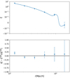 |
Fig. 3. One-dimensional two-point correlation function from HMDPL halos. Top panel: data points are the two-point correlation function estimate from the halo distribution. The solid curve is the predicted dark matter two-point correlation function scaled by |

We used our jackknife covariance matrix estimate to obtain a least-squares fit for the bias factor, which in this case gives b = 4.33 ± 0.07. Comparat et al. (2017) predicted a value of  which agrees best with the predicted bias as expected because it was calibrated on the same simulation that we used for validation. For the rest of this paper we use the model of Comparat et al. (2017) as our baseline model and treat the deviations from this as the source of the systematic uncertainty.
We then studied the effect of including halo peculiar velocities in their redshifts. In this case, the appropriate clustering statistics is the projected two-point correlation function introduced in Sect. 3. Our dark matter prediction is purely isotropic and obtained from the one-dimensional two-point correlation function by setting  . The binning in rp direction was the same as in distance r for our one-dimensional ξ(r) estimate. We chose πmin = 0h−1Mpc and πmax = 120h−1Mpc for the integral in Eq. (8). The result of this integral is the projected two-point correlation function wp(rp) shown in Fig. 4 along with the corresponding bias-scaled dark matter prediction. Because the halo sample is still the same, the mass-based bias prediction does not change compared to the one-dimensional case, but fitting the bias gives a slightly higher value of b = 4.41 ± 0.11. The difference of the predicted and measured bias is slightly larger than the 1σ uncertainty in the latter. The difference is 3% of the predicted bias, which is well within the estimated uncertainty of the b(M) model (Comparat et al. 2017).
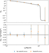 |
Fig. 4. Effect of redshift errors on the projected two-point correlation function estimate. Top panel: projected two-point correlation function from HMDPL halos. Blue data points are the two-point correlation function estimate from the halo distribution without redshift errors, and orange data points are this estimate including redshift errors. The solid curve shows the predicted dark matter two-point correlation function scaled by |

In real data, the radial cluster distances are distorted by redshift measurement errors in addition to their peculiar velocities. For a discussion of this effect, see Estrada et al. (2009), for instance. To model the effect, we measured the redshift error distribution from the CODEX clusters. Spectroscopic redshifts are available for a subset of CODEX clusters from the SDSS IV DR16 release of the SPIDERS cluster catalog (Ahumada et al. 2020). Descriptions of the survey area and spectroscopic redshift assignment are provided in Clerc et al. (2020) and Kirkpatrick et al. (2021), respectively. For areas outside of the SPIDERS footprint, redshifts were collected from public SDSS III data and several Nordic Optical Telescope (NOT) programs (PI A. Finoguenov, NOT Program IDs: 48-025, 52-026, 53-020, 51-034). The redshift assignment follows the same procedure as we used for the DR16 catalog. The number of clusters with spectroscopic redshifts is 1223, or 65% of the entire sample. We estimated the redshift error distribution as the difference between spectroscopic and photometric redshift for each cluster. We then fit this distribution with a Gaussian function of width σz and used this function to draw a random redshift error for each halo in the simulated catalog. We obtained σz = 0.0071 in the range 0.1 < z < 0.5. The effect this has on measured projected two-point correlation function is shown in Fig. 4. The corresponding measured bias of 4.29 ± 0.07, which is compatible with the bias without redshift errors and also with the predicted bias within the statistical errors. Thus we do not expect the measurement of the projected two-point correlation function to be biased by the redshift measurement errors in the CODEX catalog.
5. Clustering of CODEX clusters
Because the predicted halo bias is compatible with the measured bias for the simulated halos, we proceeded to apply the same analysis to the CODEX cluster catalog. We again estimated the projected two-point correlation function. We chose five logarithmically spaced bins over scales of 10h−1 Mpc < rp < 200h−1 Mpc and integrated over scales of 0h−1 Mpc < π < 120h−1 Mpc. We also tried using other values for πmax, but 120h−1 Mpc maximizes the clustering amplitude with minimum noise. Figure 5 shows the fitted bias as a function of πmax. To derive the covariance matrix estimates, we split the sky area into 16 jackknife subsections.
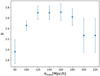 |
Fig. 5. Effect of πmax to the clustering amplitude quantified via fitted bias b. |
Figure 6 shows the projected two-point correlation function obtained from the CODEX catalog compared with dark matter two-point correlation functions scaled with the predicted bias factors based on three different mass estimates. Two estimates come from cluster X-ray luminosities (LX) using two different scaling relations, one adopted in the CODEX main paper (Finoguenov et al. 2020), and the other from Capasso et al. (2020). The third estimate comes from the cluster richness, using the summary of weak-lensing richness calibrations presented in Kiiveri et al. (2021). In Table 2 we show the mass-based bias predictions. These can be compared to the bias estimate obtained by direct fitting, which in this case is b = 3.70 ± 0.13. The richness-based mass estimates predict a bias of  which is closest to the measured value, the difference being 17% of the fitted value. The superiority of the richness-based masses is most likely due to the better quality of its measurement compared to LX based on a few counts in RASS data. Thus, we selected richness to be our baseline case in the following sections and used the deviating results from other mass estimates to illustrate an associated systematic uncertainty. To verify the robustness of our results against the rp range, we also ran the analysis in the ranges 10h−1 Mpc < rp < 100h−1 Mpc and 20h−1 Mpc < rp < 200h−1 Mpc. The results are listed in Table 3. Increasing the lower limit has a stronger effect on the fitted bias than decreasing the upper limit, but all the results are compatible within the statistical uncertainty.
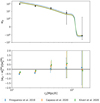 |
Fig. 6. Comparison of different cluster mass estimates. Top panel: projected two-point correlation function in redshift range 0.1 < z < 0.5. Data points are two-point correlation function estimate from CODEX clusters. The solid curves show the predicted dark matter two-point correlation function scaled by |

Predicted biases using different mass estimates.
Fitted bias using different rp ranges.
We also studied the effect of redshift binning on clustering. Figure 7 compares the CODEX clusters and predicted bias-scaled dark matter two-point correlation functions in lower 0.1 < z < 0.3 and higher 0.3 < z < 0.5 redshift samples, and for reference, also in the full range of 0.1 < z < 0.5. The corresponding comparison between predicted and fitted biases is presented in Table 4. The difference between the predicted and measured bias for the low- and high-redshift samples is 5% and 8% of the measured bias, respectively. The measured high-redshift two-point correlation function appears to deviate from the prediction at the largest scales. This might be a residual from the limitations caused by modeling the survey effects at high redshifts. We give a more detailed account of this matter in Appendix A. The predicted and measured biases are also higher for the high-redshift sample. This is expected because with increasing redshift, only massive clusters can be detected in RASS. This effect is further reinforced by our richness cut, which discards increasingly rich clusters at higher redshifts.
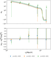 |
Fig. 7. Comparison of different redshift ranges. Top panel: projected two-point correlation function in three redshift ranges 0.1 < z < 0.5, 0.1 < z < 0.3 and 0.3 < z < 0.5. Data points are the two-point correlation function estimates from the CODEX clusters. The solid curves in corresponding colors show the predicted dark matter two-point correlation function scaled by |

Comparison of the measured and predicted biases in different redshift ranges.
A common way to characterize the amplitude of the cluster two-point correlation function is to fit a power law,
 (18)
(18)
which is found to be a good approximation at the scales ≲100 Mpc h−1 (see, e.g., Peacock & West 1992). The scale at which the correlation function crosses unity, r0, is called the correlation length, and determining its value has been the goal of many galaxy cluster studies. Collins et al. (2000) measured the correlation length from another smaller X-ray selected sample provided by the ROSAT-ESO Flux-Limited X-ray (REFLEX, Böhringer et al. 2011) survey. The value they obtained is r0 = 18.8 ± 0.9, with a slope of  over the range of 4 Mpc h−1 < r < 40 Mpc h−1. To compare with this result, we performed a least-squares fit for parameters r0 and γ. The results for our three redshift ranges are listed in Table 5. We measure a slightly steeper slope, especially for the high-redshift sample, but within the errors all the results are compatible with those of Collins et al. (2000).
Fitted power-law parameters for different redshift ranges.
6. Cosmology
As a of a proof-of-concept study, we performed a Markov chain Monte Carlo (MCMC) sampling (implemented using the emcee library3, Foreman-Mackey et al. 2013) of the matter density parameter Ωm0 and power spectrum amplitude σ8 within the ΛCDM model by comparing the two-point correlation function obtained from cluster distribution (halo distribution in case of simulations) and one obtained by scaling dark matter two-point correlation function with predicted bias. All the other cosmological parameters were fixed at values based on Wilkinson Microwave Anisotropy Probe (WMAP) nine-year results (Hinshaw et al. 2013) in the case of CODEX clusters (we later combine the posterior with one based on cluster mass function and WMAP nine-year cosmology) or Planck 2015 results in the case of HMDPL halos (the simulation was run using this cosmology). We restricted ourselves to spatially flat cosmologies so that the dark energy density parameter is determined by the matter density parameter: ΩDE0 = 1 − Ωm0 for each value of Ωm0. We assumed a Gaussian likelihood,
![Mathematical equation: $$ \begin{aligned} \ln {\mathcal{L} } = -\frac{1}{2}\left[\left(\boldsymbol{\xi }- \overline{b}^{\; 2}\boldsymbol{\xi }^\mathrm{DM} \right)^T \mathbf C ^{-1}\left(\boldsymbol{\xi }- \overline{b}^{\; 2}\boldsymbol{\xi }^\mathrm{DM} \right) + c\right], \end{aligned} $$](/articles/aa/full_html/2021/02/aa38807-20/aa38807-20-eq41.gif) (19)
(19)
where c is a constant. The predicted two-point correlation function ξDM and the mean bias  are both functions of cosmological parameters and thus updated at each MCMC step. For simplicity, we ignored the effect of errors in cluster masses on
  and on the likelihood.
The estimated two-point correlation function ξ changes with cosmology as well as with the cosmology-dependent transformation of redshifts to distances; in principle, it should therefore be reestimated at each cosmology. This effect is small, however. Figure 8 compares two-point correlation function estimates from HMDPL halos using drastically differing values of Ωm0. The fitted biases are presented in Table 6. Both of the extreme values are compatible with the central value within the statistical errors. To take the difference into account, we modeled the effect of comparing estimated and predicted two-point correlation functions computed at different cosmologies (so-called geometrical distortions, GD) following Marulli et al. (2012). Distances perpendicular and parallel to the line of sight, rp and π, are related in the two different cosmologies, labeled 1 and 2, by
 (20)
(20)
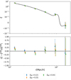 |
Fig. 8. Effect of changing Ωm0 on the two-point correlation function estimate. Top panel: bias-scaled dark matter prediction for HMDPL cosmology Ωm0 = 0.307115 (solid curve) and two-point correlation function estimates obtained using this same value and values ±0.1. Bottom panel: relative difference between the estimates and the dark matter prediction. The data points have been shifted horizontally for clarity. |
Comparison of fitted biases using different values of Ωm0 while estimating the two-point correlation function.
where DA(z) is the angular diameter distance and H(z) is the Hubble parameter at redshift z. To compare theoretical predictions at varying cosmologies with the measurement at the fiducial cosmology at scales (rp, π), we therefore evaluated them at scales (DA(z)/DA, f(z)rp,H(z)f/H(z)π), where f refers to the fiducial cosmology, and we took z to be the mean redshift of the sample.
To verify that we are able to recover the correct cosmology, we first ran the MCMC sampling using the HMDPL halo catalog. We used the same redshift, mass ranges, and binning for the projected two-point correlation function as in Sect. 4. We also included photometric redshift errors estimated from the CODEX catalog. The resulting posterior distributions of the cosmological parameters are shown in Fig. 9, displaying the full two-dimensional likelihood contours and marginalized posterior distributions for Ωm0 and σ8. The parameter values that were used to run the simulation are Ωm0 = 0.307115 and σ8 = 0.8228. The marginalized constraints we obtain are  and
and  , which are clearly compatible with the simulation cosmology.
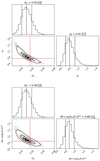 |
Fig. 9. Posterior distribution for the parameters Ωm0 and σ8 for the HMDPL catalog. The contours show the 68% and 95% confidence regions, and the values used in the simulation are shown by the dashed red lines. The dashed black lines in the marginalized posteriors show the 16%, 50%, and 84% quantiles. |
We then performed the same analysis on the CODEX clusters. All the details of the two-point correlation function estimates (such as binning) were exactly the same as described in Sect. 5. We applied flat priors in the range of 0.05 < Ωm0 < 0.5 and 0.4 < σ8 < 1.9. Figure 10 shows the posterior distributions obtained for the full CODEX cluster catalog. It favors extremely high values of σ8. The richness-to-mass scaling relation we used, however, has a quite significant uncertainty. When we take the lower 1σ extreme value for its normalization instead of the mean value, which is supported by calibrations obtained for Sunyaev–Zeldovich (SZ) clusters (Bleem et al. 2020), we obtain the posterior distribution of Fig. 11. The obtained value of σ8 is more compatible with canonical values. We adopt this 1σ lower limit as our baseline for the rest of the analysis.
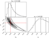 |
Fig. 10. Posterior distribution for the parameters Ωm0 and σ8 for the CODEX catalog in the full redshift range of 0.1 < z < 0.5. The contours show the 68% and 95% confidence regions, and the best fit, values are shown by the dashed red lines. The dashed black lines in the marginalized posteriors show the 16%, 50%, and 84% quantiles. |
For high values of σ8 the distributions are very flat providing poor constraints. However, Pillepich et al. (2012, 2018), for example, showed that it is possible to make the angular clustering of clusters more sensitive to the cosmology by splitting the cluster sample into redshift bins. Motivated by this, we ran the MCMC sampling using two redshift bins, 0.1 < z < 0.3 and 0.3 < z < 0.5, and computed a two-point correlation function estimate for both bins (see Fig. 7 for a display). The resulting posterior distributions for Ωm0 and σ8 are shown in Fig. 12. The distribution is in this case far less skewed toward high σ8, and we obtain marginalized parameter constraints of  and
and  (or correcting for the dependency on Ωm0,
  ). The constraints we obtain from the two redshift bins separately are
  ,
,  for the low-redshift bin and
  ,
,  for the high-redshift bin. When the two redshift bins are combined in the analysis, the constraints become tighter. However, the sampling was made assuming that the two redshifts bins are independent. This might not be the case, especially with photometric redshifts. Taking the covariance between the bins into account might loosen the constraints by some amount. For comparison with the WMAP9 cosmology, we also ran the MCMC sampling using Planck Collaboration XIII (2016) values for the fixed parameters. In this case, we obtain constraints
  and
and  . Both are compatible with values using WMAP9 cosmology within the statistical errors.
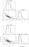 |
Fig. 12. Posterior distribution for the parameters Ωm0, σ8, and S8 for the CODEX catalog split into two redshift bins 0.1 < z < 0.3 and 0.3 < z < 0.5. The contours show the 68% and 95% confidence regions, and the best fit values are shown by the dashed red lines. The dashed black lines in the marginalized posteriors show the 16%, 50%, and 84% quantiles. |
Figures 10–12 show a strong degeneracy between Ωm0 and σ8 when clustering data alone are used. It is possible to break some of this degeneracy by combining the likelihood from the clustering analysis with that from the cluster mass function. Finoguenov et al. (2020) used the cluster X-ray luminosity function, which is essentially a proxy for their mass function, to obtain constraints Ωm0 = 0.270 ± 0.06 and σ8 = 0.79 ± 0.05. In the top panel of Fig. 13 we show the constraints we obtain by combining the two likelihoods. The individual likelihood functions are mutually nearly orthogonal, and by combining them, we can significantly tighten the parameter constraints. The bottom panel of Fig. 13 shows the marginalized posterior distributions for Ωm0 and σ8 obtained from the joint likelihood. From these we derive the parameter constraints  ,
,  . It should be noted, however, that we have estimated the joint likelihood by a simple product of the two likelihoods. This can result in an overly optimistic estimate because the two quantities involved are correlated; see, for example, Lacasa & Rosenfeld (2016), who estimated the cross-correlations of cluster counts (essentially their mass function) and galaxy power spectrum to be at ∼20% level.
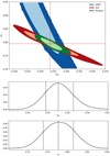 |
Fig. 13. Parameter constraints combining two-point correlation function and luminosity function likelihoods. Top panel: likelihood function of (Ωm0, σ8) from the cluster two-point correlation function (blue), X-ray luminosity function (red), and joint distribution (green). The light and dark contours are the 68% and 95% confidence regions, respectively, and the dashed red lines show the best-fit values for the joint likelihood. Bottom panel: marginalized posterior distributions for Ωm0 and σ8 obtained from the joint likelihood in the top panel. The dashed black lines show the 16%, 50%, and 84% quantiles. |
To estimate the effect of systematic uncertainties in our parameter constraints, we ran set of MCMC samplings using a variety of redshift measurements, selection functions, mass proxies, and bias-to-mass calibrations. A full account of this exercise is provided in Appendix A. We estimate the systematic error of parameter p as the sum of the squared differences between best-fit parameter values in the baseline case (presented in Fig. 12) and the comparison cases,
 (21)
(21)
where  is the best-fit value in the baseline case, and p are the best fit values for the comparison cases. We separately estimated the systematic error originating from survey effects (redshift measurement and selection function) and the systematic error from predicting the bias. The results along with the combination of the two error categories are shown in Table 7. The total systematic errors are σΩm0 = 0.02 and σσ8 = 0.23 for the two-point correlation function alone and σΩm0 = 0.07 and σσ8 = 0.04 for the combination of the two-point correlation function and the X-ray luminosity function. Both are of similar magnitude than the statistical errors in their respective cases.
Systematic errors from survey effects and bias prediction, and their combination.
A summary of our results along with a comparison with the WMAP9 and Planck 2018 results (Planck Collaboration VI 2020) is listed in Table 8. Our results from combining clustering and mass function are fully consistent with the WMAP9 results within the statistical uncertainty. A difference larger than 1σ between our values and those from Planck 2018 for Ωm0 is visible, but this difference is smaller than our estimated systematic uncertainty.
Summary of cosmological constraints obtained from the cluster two-point correlation function, two-point correlation function combined with the X-ray luminosity function, the X-ray luminosity function alone, and for CMB datasets.
All the posterior distribution corner plots in this work were plotted using the python library corner4 (Foreman-Mackey 2016).
7. Conclusions
We performed a clustering analysis on the CODEX galaxy cluster catalog. As a part of this analysis, we aimed at predicting the clustering bias of these clusters based on their masses. We first verified with a halo catalog from the HMDPL simulation that using this approach we can predict the clustering bias of dark matter halos with perfectly known masses in a known cosmology. We showed that we can recover the observed clustering bias within the statistical errors by simply averaging over the mass-based bias prediction for each individual halo in the sample. All three components in the analysis, the clustering of galaxy clusters (or dark matter halos in the case of simulations), the expected dark matter distribution, and the mass-to-bias conversion, depend on the cosmology, thus the agreement of them is a test of the cosmological model. We performed an MCMC sampling of parameters Ωm0 and σ8 to find the best-fit values by comparing the measured two-correlation function of HMDPL halos to the total matter distribution scaled by the predicted bias factor. We recovered the input cosmological parameters within the statistical uncertainty.
We applied the same analysis to the CODEX catalog. Cluster masses can be estimated from their X-ray luminosities or their richness. We determined which of these estimates of bias was best compatible with the data. We found that the mass estimates predict bias factors that agree with the measured value at a level of 17–39%; the richness-based estimates give the best agreement. We also tested how splitting the sample into redshifts bins affects the results and found that the predicted bias agrees with the measured value at the 5–17% level depending on the redshift range used. We applied the same MCMC sampling as to the HMDPL halo catalog to CODEX clusters. We found that in order to have a constraining power on σ8, we need to split the cluster sample into redshift bins (two in the case of our analysis). By binning the sample according to redshift, we obtained the following parameter constraints:  and
and  . We estimated an additional error of ±0.02 and ±0.19, respectively, that originates from systematic effects related to survey effects and bias modeling. After combining the clustering-based likelihood with one from the cluster mass function, we obtained the following parameter constraints:
  and
and  . In this case, we estimated that the systematic uncertainties contribute ±0.07 and ±0.04 additionally, respectively. It should be noted, however, that proper handling of the covariance between the two quantities would most likely loosen the constraints by some amount. In any case, our parameter constraints from clustering bias are consistent with the WMAP nine-year cosmology, and when systematic uncertainties are included, also with the Planck 2018 cosmology.
Acknowledgments
The authors wish to acknowledge CSC – IT Center for Science, Finland, for computational resources. We acknowledge grants of computer capacity from the Finnish Grid and Cloud Infrastructure (persistent identifier urn:nbn:fi:research-infras-2016072533). Based on observations made with the Nordic Optical Telescope, operated by the Nordic Optical Telescope Scientific Association at the Observatorio del Roque de los Muchachos, La Palma, Spain, of the Instituto de Astrofisica de Canarias. The authors gratefully acknowledge the Gauss Centre for Supercomputing e.V. (www.gauss-centre.eu) and the Partnership for Advanced Supercomputing in Europe (PRACE, www.prace-ri.eu) for funding the MultiDark simulation project by providing computing time on the GCS Supercomputer SuperMUC at Leibniz Supercomputing Centre (LRZ, www.lrz.de). Funding for the Sloan Digital Sky Survey IV has been provided by the Alfred P. Sloan Foundation, the U.S. Department of Energy Office of Science, and the Participating Institutions. SDSS-IV acknowledges support and resources from the Center for High-Performance Computing at the University of Utah. The SDSS web site is www.sdss.org. SDSS-IV is managed by the Astrophysical Research Consortium for the Participating Institutions of the SDSS Collaboration including the Brazilian Participation Group, the Carnegie Institution for Science, Carnegie Mellon University, the Chilean Participation Group, the French Participation Group, Harvard-Smithsonian Center for Astrophysics, Instituto de Astrofísica de Canarias, The Johns Hopkins University, Kavli Institute for the Physics and Mathematics of the Universe (IPMU)/University of Tokyo, the Korean Participation Group, Lawrence Berkeley National Laboratory, Leibniz Institut für Astrophysik Potsdam (AIP), Max-Planck-Institut für Astronomie (MPIA Heidelberg), Max-Planck-Institut für Astrophysik (MPA Garching), Max-Planck-Institut für Extraterrestrische Physik (MPE), National Astronomical Observatories of China, New Mexico State University, New York University, University of Notre Dame, Observatário Nacional/MCTI, The Ohio State University, Pennsylvania State University, Shanghai Astronomical Observatory, United Kingdom Participation Group, Universidad Nacional Autónoma de México, University of Arizona, University of Colorado Boulder, University of Oxford, University of Portsmouth, University of Utah, University of Virginia, University of Washington, University of Wisconsin, Vanderbilt University, and Yale University.
References
- Ahumada, R., Allende, P., Carlos, A. P., et al. 2020, ApJS, 249, 3 [CrossRef] [Google Scholar]
- Allevato, V., Finoguenov, A., Cappelluti, N., et al. 2011, ApJ, 736, 99 [NASA ADS] [CrossRef] [Google Scholar]
- Allevato, V., Finoguenov, A., Hasinger, G., et al. 2012, ApJ, 758, 47 [NASA ADS] [CrossRef] [Google Scholar]
- Annalisa Mana, A., Giannantonio, T., & Weller, J. 2013, MNRAS, 434, 684 [NASA ADS] [CrossRef] [Google Scholar]
- Bhattacharya, S., Heitmann, K., White, M., et al. 2011, ApJ, 732, 122 [NASA ADS] [CrossRef] [Google Scholar]
- Bleem, L. E., Bocquet, S., Stalder, B., et al. 2020, ApJS, 247, 25 [CrossRef] [Google Scholar]
- Böhringer, H., Schuecker, P., Guzzo, L., et al. 2011, A&A, 369, 826 [Google Scholar]
- Capasso, R., Mohr, J. J., Saro, A., et al. 2019, MNRAS, 486, 1594 [CrossRef] [Google Scholar]
- Capasso, R., Mohr, J. J., Saro, A., et al. 2020, MNRAS, 494, 2736 [CrossRef] [Google Scholar]
- Cavaliere, A., & Fusco-Femiano, R. 1976, A&A, 49, 137 [NASA ADS] [Google Scholar]
- Clerc, N., Merloni, A., Zhang, Y.-Y., et al. 2016, MNRAS, 463, 4490 [NASA ADS] [CrossRef] [Google Scholar]
- Clerc, N., Kirkpatrick, C. C., Finoguenov, A., et al. 2020, MNRAS, 497, 3976 [CrossRef] [Google Scholar]
- Collins, C. A., Guzzo, L., Böhringer, H., et al. 2000, MNRAS, 319, 939 [NASA ADS] [CrossRef] [Google Scholar]
- Comparat, J., Prada, F., Yepes, G., & Klypin, A. 2017, MNRAS, 469, 4157 [CrossRef] [Google Scholar]
- Comparat, J., Merloni, A., Salvato, M., et al. 2019, MNRAS, 487, 2005 [NASA ADS] [CrossRef] [Google Scholar]
- Comparat, J., Eckert, D., Finoguenov, A., et al. 2020, Open J. Astrophys., 3, 13 [CrossRef] [Google Scholar]
- Davis, M., & Peebles, P. J. E. 1983, ApJ, 267, 465 [NASA ADS] [CrossRef] [Google Scholar]
- Diemer, B. 2018, ApJS, 239, 13 [NASA ADS] [CrossRef] [Google Scholar]
- Estrada, J., Sefusatti, E., & Frieman, J. A. 2009, ApJ, 692, 265 [NASA ADS] [CrossRef] [Google Scholar]
- Eisenstein, D. J., & Hu, W. 1998, ApJ, 496, 605 [NASA ADS] [CrossRef] [Google Scholar]
- Eisenstein, D. J., & Hu, W. 1999, ApJ, 511, 5 [NASA ADS] [CrossRef] [Google Scholar]
- Farahi, A., Mulroy, S. L., Evrard, A. E., et al. 2019, Nature Com., 10, 2504 [CrossRef] [Google Scholar]
- Finoguenov, A., Rykoff, E., Clerc, N., et al. 2020, A&A, 638, A114 [CrossRef] [EDP Sciences] [Google Scholar]
- Foreman-Mackey, D. 2016, J. Open Source Softw., 1, 24 [Google Scholar]
- Foreman-Mackey, D., Hogg, D. W., Lang, D., & Goodman, J. 2013, PASP, 125, 306 [Google Scholar]
- Hinshaw, G., Larson, D., Komatsu, E., et al. 2013, ApJS, 208, 19 [NASA ADS] [CrossRef] [Google Scholar]
- Jimeno, P., Broadhurst, T., Lazkoz, R., et al. 2017, MNRAS, 466, 2658 [CrossRef] [Google Scholar]
- Käfer, F., Finoguenov, A., Eckert, D., et al. 2019, A&A, 628, A43 [NASA ADS] [CrossRef] [EDP Sciences] [Google Scholar]
- Kiiveri, K., Gruen, D., Finoguenov, A., et al. 2021, MNRAS, in press, [arXiv:2101.02257] [Google Scholar]
- Kirkpatrick, C. C., Clerc, N., Finoguenov, A., et al. 2021, MNRAS, submitted, [arXiv:2101.04695] [Google Scholar]
- Klein, M., Grandis, S., Mohr, J. J., et al. 2019, MNRAS, 488, 739 [CrossRef] [Google Scholar]
- Klypin, A., Yepes, G., Gottlöber, S., Prada, F., & Heß, S. 2016, MNRAS, 457, 4340 [NASA ADS] [CrossRef] [Google Scholar]
- Koester, B. P., McKay, T. A., Annis, J., et al. 2007, ApJ, 660, 239 [NASA ADS] [CrossRef] [Google Scholar]
- Lacasa, F., & Rosenfeld, R. 2016, J. Cosmol. Astropart. Phys., 8, 005 [CrossRef] [Google Scholar]
- Landy, S. D., & Szalay, A. S. 1993, ApJ, 412, 64 [NASA ADS] [CrossRef] [Google Scholar]
- Lewis, A., Challinor, A., & Lasenby, A. 2000, ApJ, 538, 473 [Google Scholar]
- Marulli, F., Bianchi, D., Branchini, E., et al. 2012, MNRAS, 426, 2566 [NASA ADS] [CrossRef] [Google Scholar]
- Marulli, F., Veropalumbo, A., & Moresco, M. 2016, Astron. Comput., 14, 35 [NASA ADS] [CrossRef] [Google Scholar]
- Marulli, F., Veropalumbo, A., Sereno, M., et al. 2018, A&A, 620, A1 [NASA ADS] [CrossRef] [EDP Sciences] [Google Scholar]
- Mo, H. J., & White, S. D. M. 1996, MNRAS, 282, 347 [NASA ADS] [CrossRef] [Google Scholar]
- Mulroy, S. L., Farahi, A., Evrard, A. E., et al. 2019, MNRAS, 484, 60 [NASA ADS] [CrossRef] [Google Scholar]
- Navarro, J. F., Frenk, C. S., & White, S. D. M. 1997, ApJ, 490, 493 [NASA ADS] [CrossRef] [Google Scholar]
- Peacock, J. A., & West, M. J. 1992, MNRAS, 259, 494 [NASA ADS] [CrossRef] [Google Scholar]
- Pierre, M., Pacaud, F., Adami, C., et al. 2016, A&A, 592, A1 (XXL Paper I) [NASA ADS] [CrossRef] [EDP Sciences] [Google Scholar]
- Pillepich, A., Porciani, C., & Reiprich, T. H. 2012, MNRAS, 422, 44 [Google Scholar]
- Pillepich, A., Reiprich, T. H., Porciani, C., et al. 2018, MNRAS, 481, 613 [NASA ADS] [CrossRef] [Google Scholar]
- Planck Collaboration XVI. 2014, A&A, 571, A16 [NASA ADS] [CrossRef] [EDP Sciences] [Google Scholar]
- Planck Collaboration XIII. 2016, A&A, 594, A13 [NASA ADS] [CrossRef] [EDP Sciences] [Google Scholar]
- Planck Collaboration VI. 2020, A&A, 641, A6 [NASA ADS] [CrossRef] [EDP Sciences] [Google Scholar]
- Prada, F., Klypin, A. A., Cuesta, A. J., Betancort-Rijo, J. E., & Primack, J. 2012, MNRAS, 423, 3018 [NASA ADS] [CrossRef] [Google Scholar]
- Rykoff, E. S., Rozo, E., Busha, M. T., et al. 2014, ApJ, 785, 104 [NASA ADS] [CrossRef] [Google Scholar]
- Schuecker, P., Guzzo, L., Collins, C. A., et al. 2002, MNRAS, 335, 807 [NASA ADS] [CrossRef] [EDP Sciences] [Google Scholar]
- Sheth, R. K., & Tormen, G. 1999, MNRAS, 308, 119 [NASA ADS] [CrossRef] [Google Scholar]
- Sheth, R. K., Mo, H. J., & Tormen, G. 2001, MNRAS, 323, 1 [NASA ADS] [CrossRef] [Google Scholar]
- Tinker, J. L., Robertson, B. E., Kravtsov, A. V., et al. 2010, ApJ, 724, 878 [NASA ADS] [CrossRef] [Google Scholar]
Appendix A: Systematic effects
We report the different systematic effects in the cosmological parameter constraints we obtain. Our baseline case is the one where we split the CODEX sample in two redshift bins 0.1 < z < 0.3 and 0.3 < z < 0.5 and use richness-based mass estimates and the b(M) model from Comparat et al. (2017). We compared the best-fit parameter values for Ωm0 and σ8 from MCMC samplings by varying survey effects, mass estimates, and the b(M) model. All of the best-fit parameter values we obtain for different comparison cases are summarized in Table A.3.
As mentioned in Sect. 4, a subset of CODEX clusters has spectroscopic redshifts associated with them in addition to photometric redshifts. To verify the robustness of the photometric redshifts, we computed the two-point correlation function using spectroscopic redshifts when available and photometric redshifts for the remaining clusters. A comparison between measured and predicted correlation functions in the full redshift range is presented in Fig. A.1, where we also show the results for a purely spectroscopic sample limited to the SDSS DR16 area. In this case, we have a slightly smaller set of spectroscopic redshifts (880 within 0.1 < z < 0.5) because we required spectroscopic completeness. The measured and predicted biases for both cases in all the redshift bins are listed in Table A.1. At lower redshifts, the measured biases are compatible with those from the purely photometric sample, but at higher redshifts, there is some difference.
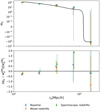 |
Fig. A.1. Comparison of photometric, mixed, and spectroscopic redshifts. Top panel: projected two-point correlation functions in the redshift range 0.1 < z < 0.5. Data points are the two-point correlation function estimate from CODEX clusters. The solid curve is the predicted dark matter two-point correlation function scaled by |

Bias values obtained for a mixture of photometric and spectroscopic redshifts (column bmix) and those of a purely photometric sample (column bphz), and a purely spectroscopic sample (columns bspe) as well as the mass-based prediction (column  ) from Table 4.
In Fig. 7 the slope of the measured correlation function in the high-redshift bin and at large scales appears to be flatter than the prediction and the low-redshift bin. To test whether this is due to an incorrect characterization of the selection function, we ran the analysis forcing the redshift distribution of the random catalog to be exactly that of the data catalog in redshift bins of Δz = 0.027. Another test we ran was to use the subregion of the CODEX survey area in which the X-ray sensitivity is uniform. A comparison of the fitted biases obtained using different selection functions is given in Table A.2. Figure A.2 shows the two-point correlation function results in a high-z bin using different selection functions. They show that the flattening of the measured two-point correlation function at large scales at high redshifts occurs regardless of the selection function used, and we therefore suspect that this is not the cause of the effect. The effect of redshift errors and selection function on the cosmological parameter constraints is demonstrated by the corresponding changes in the best-fit parameter values presented in Table A.3.
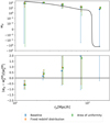 |
Fig. A.2. Comparison of different selection functions in high-z bin. Top panel: projected two-point correlation function in redshift range 0.3 < z < 0.5. Data points are the two-point correlation function estimate from CODEX clusters. The solid curve shows the predicted dark matter two-point correlation function scaled by |

Comparison of fitted and predicted biases using different selection functions.
Best-fit parameter values for all the cases used to compute the systematic error on the parameters Ωm0 and σ8.
In addition to different survey effects, we studied the effect of varying the mass and bias estimates. We ran MCMC sampling using the two X-ray luminosity based mass calibrations (introduced in Sect. 5). From the bias models b(M) in Table 1 we chose the two that gave the most extreme values, that is, Tinker et al. (2010) and Bhattacharya et al. (2011), to be compared with the baseline case. The resulting shifts in the best-fit parameter values are shown again in Table A.3.
All Tables
Comparison of fitted biases using different values of Ωm0 while estimating the two-point correlation function.
Systematic errors from survey effects and bias prediction, and their combination.
Summary of cosmological constraints obtained from the cluster two-point correlation function, two-point correlation function combined with the X-ray luminosity function, the X-ray luminosity function alone, and for CMB datasets.
Bias values obtained for a mixture of photometric and spectroscopic redshifts (column bmix) and those of a purely photometric sample (column bphz), and a purely spectroscopic sample (columns bspe) as well as the mass-based prediction (column ) from Table 4.
Comparison of fitted and predicted biases using different selection functions.
Best-fit parameter values for all the cases used to compute the systematic error on the parameters Ωm0 and σ8.
All Figures
|
Fig. 1. Sky footprint of the subset of the CODEX catalog used to compute the two-point correlation function. Orange points show the clusters, and blue points show the random points. |
| In the text | |
|
Fig. 2. Redshift distribution (dn/dz) of the subset of the CODEX catalog used to compute the two-point correlation function along with the corresponding random catalog. The area of the two histograms is normalized to 1. |
| In the text | |
|
Fig. 3. One-dimensional two-point correlation function from HMDPL halos. Top panel: data points are the two-point correlation function estimate from the halo distribution. The solid curve is the predicted dark matter two-point correlation function scaled by |
| In the text | |
|
Fig. 4. Effect of redshift errors on the projected two-point correlation function estimate. Top panel: projected two-point correlation function from HMDPL halos. Blue data points are the two-point correlation function estimate from the halo distribution without redshift errors, and orange data points are this estimate including redshift errors. The solid curve shows the predicted dark matter two-point correlation function scaled by |
| In the text | |
|
Fig. 5. Effect of πmax to the clustering amplitude quantified via fitted bias b. |
| In the text | |
|
Fig. 6. Comparison of different cluster mass estimates. Top panel: projected two-point correlation function in redshift range 0.1 < z < 0.5. Data points are two-point correlation function estimate from CODEX clusters. The solid curves show the predicted dark matter two-point correlation function scaled by |
| In the text | |
|
Fig. 7. Comparison of different redshift ranges. Top panel: projected two-point correlation function in three redshift ranges 0.1 < z < 0.5, 0.1 < z < 0.3 and 0.3 < z < 0.5. Data points are the two-point correlation function estimates from the CODEX clusters. The solid curves in corresponding colors show the predicted dark matter two-point correlation function scaled by |
| In the text | |
|
Fig. 8. Effect of changing Ωm0 on the two-point correlation function estimate. Top panel: bias-scaled dark matter prediction for HMDPL cosmology Ωm0 = 0.307115 (solid curve) and two-point correlation function estimates obtained using this same value and values ±0.1. Bottom panel: relative difference between the estimates and the dark matter prediction. The data points have been shifted horizontally for clarity. |
| In the text | |
|
Fig. 9. Posterior distribution for the parameters Ωm0 and σ8 for the HMDPL catalog. The contours show the 68% and 95% confidence regions, and the values used in the simulation are shown by the dashed red lines. The dashed black lines in the marginalized posteriors show the 16%, 50%, and 84% quantiles. |
| In the text | |
|
Fig. 10. Posterior distribution for the parameters Ωm0 and σ8 for the CODEX catalog in the full redshift range of 0.1 < z < 0.5. The contours show the 68% and 95% confidence regions, and the best fit, values are shown by the dashed red lines. The dashed black lines in the marginalized posteriors show the 16%, 50%, and 84% quantiles. |
| In the text | |
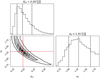 |
Fig. 11. Same as Fig. 10, but with the richness-to-mass scaling relation with 1σ deviation. |
| In the text | |
|
Fig. 12. Posterior distribution for the parameters Ωm0, σ8, and S8 for the CODEX catalog split into two redshift bins 0.1 < z < 0.3 and 0.3 < z < 0.5. The contours show the 68% and 95% confidence regions, and the best fit values are shown by the dashed red lines. The dashed black lines in the marginalized posteriors show the 16%, 50%, and 84% quantiles. |
| In the text | |
|
Fig. 13. Parameter constraints combining two-point correlation function and luminosity function likelihoods. Top panel: likelihood function of (Ωm0, σ8) from the cluster two-point correlation function (blue), X-ray luminosity function (red), and joint distribution (green). The light and dark contours are the 68% and 95% confidence regions, respectively, and the dashed red lines show the best-fit values for the joint likelihood. Bottom panel: marginalized posterior distributions for Ωm0 and σ8 obtained from the joint likelihood in the top panel. The dashed black lines show the 16%, 50%, and 84% quantiles. |
| In the text | |
|
Fig. A.1. Comparison of photometric, mixed, and spectroscopic redshifts. Top panel: projected two-point correlation functions in the redshift range 0.1 < z < 0.5. Data points are the two-point correlation function estimate from CODEX clusters. The solid curve is the predicted dark matter two-point correlation function scaled by |
| In the text | |
|
Fig. A.2. Comparison of different selection functions in high-z bin. Top panel: projected two-point correlation function in redshift range 0.3 < z < 0.5. Data points are the two-point correlation function estimate from CODEX clusters. The solid curve shows the predicted dark matter two-point correlation function scaled by |
| In the text | |
Current usage metrics show cumulative count of Article Views (full-text article views including HTML views, PDF and ePub downloads, according to the available data) and Abstracts Views on Vision4Press platform.
Data correspond to usage on the plateform after 2015. The current usage metrics is available 48-96 hours after online publication and is updated daily on week days.
Initial download of the metrics may take a while.