| Issue |
A&A
Volume 642, October 2020
|
|
|---|---|---|
| Article Number | A76 | |
| Number of page(s) | 14 | |
| Section | Interstellar and circumstellar matter | |
| DOI | https://doi.org/10.1051/0004-6361/202037721 | |
| Published online | 06 October 2020 | |
Fragmentation of star-forming filaments in the X-shaped nebula of the California molecular cloud★
1
National Astronomical Observatories, Chinese Academy of Sciences,
Beijing
100101, PR China
e-mail: This email address is being protected from spambots. You need JavaScript enabled to view it.
2
Laboratoire d’Astrophysique (AIM), CEA/DRF, CNRS, Université Paris-Saclay, Université Paris Diderot, Sorbonne Paris Cité, 91191
Gif-sur-Yvette, France
e-mail: This email address is being protected from spambots. You need JavaScript enabled to view it.
; This email address is being protected from spambots. You need JavaScript enabled to view it.
3
University of Chinese Academy of Sciences, Beijing 100049, PR China
4
Kavli Institute for Astronomy and Astrophysics, Peking University, 5 Yiheyuan Road, Haidian District,
Beijing 100871, PR China
5
European Southern Observatory (ESO) Headquarters, Karl-Schwarzschild-Str. 2,
85748 Garching bei München, Germany
Received:
13
February
2020
Accepted:
27
July
2020
Abstract
Context. Dense molecular filaments are central to the star formation process, but the detailed manner in which they fragment into prestellar cores is not well understood yet.
Aims. Here, we investigate the fragmentation properties and dynamical state of several star-forming filaments in the X-shaped nebula region of the California molecular cloud in an effort to shed some light on this issue.
Methods. We used multiwavelength far-infrared images from Herschel as well as the getsources and getfilaments extraction methods to identify dense cores and filaments in the region and derive their basic properties. We also used a map of 13CO(2−1) emission from the Arizona 10m Submillimeter Telescope (SMT) to constrain the dynamical state of the filaments.
Results. We identified ten filaments with aspect ratios of AR > 4 and column density contrasts of C > 0.5, as well as 57 dense cores, including two protostellar cores, 20 robust prestellar cores, 11 candidate prestellar cores, and 24 unbound starless cores. All ten filaments have roughly the same deconvolved full width at half maximum (FWHM), with a median value of 0.12 ± 0.03 pc, which is independent of their column densities ranging from <1021 cm−2 to >1022 cm−2. Two star-forming filaments (# 8 and # 10) stand out since they harbor quasi-periodic chains of dense cores with a typical projected core spacing of ~0.15 pc. These two filaments have thermally supercritical line masses and are not static. Filament 8 exhibits a prominent transverse velocity gradient, suggesting that it is accreting gas from the parent cloud gas reservoir at an estimated rate of ~40 ± 10 M⊙ Myr−1 pc−1. Filament 10 includes two embedded protostars with outflows and it is likely at a somewhat later evolutionary stage than filament 8. In both cases, the observed (projected) core spacing is similar to the filament width and significantly shorter than the canonical separation of ~4 times the filament width predicted by classical cylinder fragmentation theory. It is unlikely that projection effects can explain this discrepancy. We suggest that the continuous accretion of gas onto the two star-forming filaments, as well as the geometrical bending of the filaments, may account for the observed core spacing.
Conclusions. Our findings suggest that the characteristic fragmentation lengthscale of molecular filaments is quite sensitive to external perturbations from the parent cloud, such as the gravitational accretion of ambient material.
Key words: stars: formation / ISM: clouds / dust, extinction / ISM: kinematics and dynamics
The reduced 12CO datacube is only available at the CDS via anonymous ftp to cdsarc.u-strasbg.fr (130.79.128.5) or via http://cdsarc.u-strasbg.fr/viz-bin/cat/J/A+A/642/A76
© ESO 2020
1 Introduction
The early phases of star formation are still poorly understood. One of the most pressing open questions is how filaments fragment into cores at the earliest evolutionary stages. Addressing this issue is crucial to our understanding of the initial conditions of star formation (cf. André et al. 2010).
Observations with the Herschel space observatory have revealed that filaments are truly ubiquitous in the cold interstellar medium (ISM), with lengths ranging from ~1 pc in nearby molecular clouds to ~102 pc in the Galactic plane (Men’shchikov et al. 2010; Wang et al. 2015). Most (>75%) prestellar cores lie inside filaments with column densities of  (Könyves et al. 2015), implying that filaments play a key role in the star formation process (André et al. 2014). The typical inner width of filaments in nearby molecular clouds is ~0.1 pc (Arzoumanian et al. 2011, 2019), but the origin of this characteristic width is still a controversial topic. The typical value may come from supersonic turbulence in the ISM (Pudritz & Kevlahan 2013; Federrath 2016) or the balance of a quasi-equilibrium structure with ambient ISM pressure (Fischera & Martin 2012). Filaments serve as highly efficient routes for feeding material into star-forming cores (André et al. 2014). The material around filaments is not at all static. For instance, a pronounced transverse velocity gradient provides good kinematic evidence for accretion flows of ambient gas material into the B211/B213 filament of the Taurus molecular cloud (MC) (Palmeirim et al. 2013; Shimajiri et al. 2019b). Other dense filaments, such as infrared dark clouds or the Serpens South filament, exhibit both transverse and longitudinal velocity gradients, suggesting that gas is not only accreted by, but also flowing along these filaments (e.g., Kirk et al. 2013). In most cases, the transverse gradients appear to dominate over the longitudinal gradients (Dhabal et al. 2018). In the Serpens South case, for instance, the mass flow rate along the filament is estimated to be only ~ 1/4 of the accretion rate in the transverse direction (Kirk et al. 2013). The critical line mass of a cylindrical isothermal filament in hydrostatic equilibrium is
  , where cs is the sound speed and G is the gravitational constant, or ~16 M⊙ pc−1 for a gas temperature of 10 K (e.g., Ostriker 1964; Inutsuka & Miyama 1997). Recently, Arzoumanian et al. (2019) divided observed filaments into the following three categories according to their line mass Mline: thermally supercritical filaments (Mline ≳ 2 Mline, crit), transcritical filaments (0.5 Mline, crit ≲ Mline ≲ 2 Mline, crit), and thermally subcritical filaments (Mline, crit ≲ 0.5 Mline, crit). For an infinitely long cylindrical filament in hydrostatic equilibrium, core spacing is predicted to be ~ 4× the filamentdiameter by linear fragmentation models (e.g., Inutsuka & Miyama 1992), or ~ 0.4 pc taking the typical filament width into account. However, this does not match the actual core spacing found in observations which, at least on small scales, appears to be dominated by typical Jeans-like fragmentation (e.g., Kainulainen et al. 2013, 2017; Könyves et al. 2020; Ladjelate et al. 2020). Here, based on our findings in the California MC, we propose that this discrepancy results from the fact that star-forming filaments are not isolated but they accrete fresh matter from their parent clouds at the same time as they fragment into cores.
Star formation activity is generally only found in high-extinction parts of MCs. The mass of high-extinction material with AK > 1.0 mag in the California MC is only 10% of that in OrionA MC (Lada et al. 2009), and the star formation rate is accordingly much lower. The number of young stellar objects (YSOs), which may be taken as an indicator of star-formation activity, is only 177/2980 ~ 6% of that observed in the Orion A MC (Lada et al. 2017; Großschedl et al. 2019). Only one B-type main-sequence star is found in the southeastern part of the California MC and it is associated with relatively intense star formation in a local region around it (Andrews & Wolk 2008). The global star formation efficiency estimated by Zhang et al. (2018) for the California MC is only ~ 1%, which is half of the typical value (~2%) in the molecular clouds of the Milky Way (Evans 1991). The California MC is therefore an ideal place to study star formation at early stages. The X-shaped region lies at the center of the California MC (see Fig. 1). The distance to the California MC, as estimated from Gaia DR2 (Gaia Collaboration 2018) stellar parallaxes, is 500 ± 7 pc according to Yan et al. (2019) and 470 ± 24 pc according to Zucker et al. (2019). This is slightly farther than both the distance (450 ± 23 pc) estimated by Lada et al. (2009) through the comparison of foreground star counts with Galactic models and the distance (410 ± 41 pc) estimated by Schlafly et al. (2014) with stars from the PanSTARRS-1 survey. Different distance measurement methods bring uncertainties of about 10% in size and 20% in mass for the California MC. In this study, we adopt a distance of 500 pc. The most distinctive feature of this region is that it resembles an “X”. Two low-density filaments meet at the north dense hub region and extend to the southeast and southwest with an intersection angle of ~ 60° in the plane of sky. Small longitudinal velocity gradients of 0.1 and 0.2 km s−1 pc−1 are measured along the southeast and southwest filaments (Imara et al. 2017). The hub region harbors at least two YSOs. One is a Class II object and the other is a Class I source (Harvey et al. 2013; Broekhoven-Fiene et al. 2014). These two YSOs may be the driving sources of a low-mass low-velocity outflow (Imara et al. 2017).
The outline of the present paper is as follows. In Sect. 2, we describe the Herschel submillimeter dust emission data and SMT 10m molecular line observations of the X-shaped region. Data analysis and results are presented in Sect. 3. In Sect. 4, we discuss evidence of accretion onto an early-stage filament as well as the detailed fragmentation properties of the same filament. We summarize our conclusions in Sect. 5.
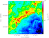 |
Fig. 1 Large-scale column density map of the California MC derived from Planck 850 μm optical-depth data (5′ resolution). The location of the X-shaped nebula region is marked with a black square. |
2 Observations and data reduction
2.1 Herschel dust continuum data
The Herschel imaging observations of the California MC (Harvey et al. 2013) include PACS 70 and 160 μm (Poglitsch et al. 2010) as well as SPIRE 250, 350, and 500 μm (Griffin et al. 2010) data. The beam sizes of the PACS data at 70 and 160 μm are 8.4″ and 13.5″, respectively. The beam sizes of the SPIRE data at 250, 350, and 500 μm are 18.2″, 24.9″, and 36.3″, respectively.The SPIRE/PACS parallel-mode was used to make scan maps with a speed of 60″ s−1. We downloaded the Herschel maps from the NASA/IPAC Infrared Science Archive1 and extracted a subfield of about 40′ × 40′ around the X-shaped nebula. A close-up map of the X-shaped nebula is shown in Fig. 2. The location of the X-shaped nebula is marked in the large-scale map of the California MC shown in Fig. 1. Zero-level offsets were derived for the Herschel maps from a comparison with Planck and IRAS data (cf. Bracco et al., in prep.; Bernard et al. 2010). They are 19.7, 26.5, 15.0, and 5.5 MJy sr−1 at 160, 250, 350, and 500 μm, respectively. Pixel-by-pixel SED fitting to the Herschel 160–500 μm data with a modified blackbody function was used to create a high-resolution (18.2″) H2 column density map with the method described in Appendix A of Palmeirim et al. (2013). A power-law form was assumed for the dust opacity,  , with a fixed β = 2 value (Roy et al. 2014). Our column density map has a resolution that is twice as high as the 36.3″-resolution map presented by Harvey et al. (2013). When smoothed to the same 5′ resolution, our high-resolution map is consistent within better than 10% for over more than 90% of the pixels with the Planck 850 μm optical-depth map converted to an H2 column density image using the above dust opacity law. A temperature-corrected 160 μm map was also derived by converting the original 160 μm map to an approximate column density image using the color-temperature map derived from the intensity ratio between 160 and 250 μm (see Könyves et al. 2015).
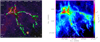 |
Fig. 2 Blow-up column density views of the X-shaped nebula region in the California MC. Panel A: filtered version of the high-resolution (18.2″) column density map, showing partially-reconstructed filaments with transverse angular scales only up to ~ 100″ from getfilaments (cf. Sect. 2.4.3 in Men’shchikov 2013). The background image shows field stars from the Pan-STARRS optical survey (Chambers et al. 2016). Panel B: unfiltered high-resolution column density map with the network of filamentary structures identified by getfilaments overlaid in white. The crests of the ten filaments selected in Sect. 3.2 are highlighted in black and magenta for thermally supercritical filaments with Mline >Mline,crit and subcritical filaments with Mline < Mline,crit, respectively. |
2.2 SMT 10m single-dish observations of CO lines
Maps of the X-shaped nebula in the 12CO(2−1) and 13CO(2−1) lines were obtained from the ESO Public Survey SAMPLING2 (Wang et al. 2018). These CO observations were carried out with the 10 m submillimeter telescope (SMT) of the Arizona Radio Observatory in on-the-fly mode with Nyquist sampling, and they cover thirteen 5′ × 5′ subfields arranged along the main “X” of the X-shaped region (see Fig. A.1). We used GILDAS3 to detect bad channels and calibrate the data. A main beam efficiency of 0.7 was adopted to convert the measured antenna temperature (TA) scale to a main beam temperature(Tmb) scale. The effective resolution of the CO data is 36″, which corresponds to ~0.09 pc at the distance of 500 pc. The velocity resolution (channel width) is 0.33 km s−1, the root mean square (rms) noise is less than 0.2 K, and the pixel size of the final data cubes is 8″.
3 Data analysis and results
The Herschel 70, 160, 250, 350, and 500 μm images, complemented by the temperature-corrected 160 μm image (at 13.5″ resolution) and the H2 column density image (at 18.2″ resolution), were reprojected onto the same 3″ pixel grid covering the same area of ~ 0.4 deg2 (cf. Fig. 2B and black square in Fig. 1).
3.1 Source and filament extraction
Before the extraction of sources and filaments, all original images were processed with the getimages algorithm (Men’shchikov 2017) to produce simpler, flatter detection images after subtraction of the large-scale background. This algorithm equalizes the background and noise fluctuations across an entire image, making extractions more reliable and less prone to spurious sources. The resulting flattened detection images were given as input to getsources (Men’shchikov et al. 2012), a multiwavelength, multi-scale source extraction package, which also includes the filament extraction algorithm getfilaments (Men’shchikov 2013). The getsources and getfilaments algorithms only have one user-defined parameter per image, which is the maximum size of the sources of interest (see, e.g., Sect 3.2 in Men’shchikov 2017). Here, source extraction was performed4 using a maximum size of four times the angular resolution at each wavelength.
Both getsources and getfilaments employ spatial decomposition to process and analyze the entire multiwavelength data set. The decomposed images are cleaned of all insignificant fluctuations and combined together to detect sources in all wavebands simultaneously. After having detected the sources, getsources measures their properties (e.g., fluxes, sizes) at each wavelength in the original images. To identify the self-luminous point-like sources, a second extraction run, which only uses the 70 μm image to detect sources, is performed, measuring the fluxes of all detections in each waveband. Here, the high-resolution column density image (18.2″) was processed by getfilaments to detect the filaments (their skeletons) and then to measure and catalog their properties. For full details on how getsources and getfilaments work, we refer the interested readers to the papers by Men’shchikov et al. (2012) and Men’shchikov (2013, 2017), which also include links to the numerical codes.
3.2 Filamentary structure selection
Molecular filaments are elongated structures of gas and dust in molecular clouds (e.g., André et al. 2014; André 2017). We define the aspect ratios (AR) of a filamentary structure as
 (1)
(1)
where L is length of the crest and W is the full width at half maximum (FWHM) of the radial column density profile. We use the median FWHM measured along the crest in the present study. The column density contrast (C) of a filamentary structure is defined as
 (2)
(2)
where  is the median column density along the filament crest and
  is the background column density around the filament. We note that
  is measured in the source-subtracted filament map, while
  is measured in the background map. Using getfilaments, a network of filaments and its corresponding skeleton was traced in the column density map. From this network, we selected ten filamentary structures with aspect ratios of AR > 4 and column density contrasts of C > 0.5. The line mass Mline of each filament was estimated as follows:
 (3)
(3)
where  is the molecular weight per hydrogen molecule and mH is the H atom mass. Assuming that each filament is cylindrical, we considered the filament diameter to be the measured filament FWHM, W. The filament average volume density was estimated as
 (4)
(4)
We identified five subcritical filaments (filament 1–4, 7) and five supercritical (or transcritical) filaments (filament 5, 6, 8–10). Figure 3 shows the radial column density profile (panel a) and the temperature profile (panel b) of filament 8, as was measured in the original column density and dust temperature maps, respectively. The estimated background column density toward this filament is ~ 3 × 1021 cm2 and the centroid temperatureis ~13 K. Likewise, Fig. 4 shows the radial column density and temperature profiles of filament 10. The derived physical properties of the ten selected filaments are given in Table 1. The deconvolved FWHM (Wdec) of the filaments range from 0.09 to 0.18 pc and they are largely uncorrelated with the filament column densities ( ) (see Fig. 5a).
The median filament width Wdec is 0.12 ± 0.03 pc, which is consistent with the commoninner width Wdec ~ 0.1 pc of filaments in the Herschel Gould Belt survey (HGBS; see e.g., Arzoumanian et al. 2011, 2019). The median column density contrast over the background is C ~ 0.9 ± 0.2 for the low-density subcritical filaments and C ~ 4 ± 0.7 for the higher-density supercritical (or transcritical) filaments. Clearly, the lower contrast of subcritical filaments leads to larger measurement errors and larger uncertainties in their derived properties, such as their widths. The median line mass of subcritical filaments is  , while that of supercritical (or transcritical) filaments is
  . The median volume density of subcritical filaments is estimated to be
  , while that of supercritical (or transcritical) filaments is
  . As the filament width Wdec is nearly uniform, both
  and
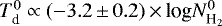
and  scale linearly with Mline, according to Eqs. (3) and (4). The central dust temperature Td of each filament was estimated from the dust temperature map (at 36.3″ resolution) along the filament crest. This dust temperature Td is anti-correlated with
  :
:  (see Fig. 5b). The median dust temperature of subcritical filaments is
  K and that of supercritical (or transcritical) filaments is 3 K lower,
  K. For filaments that only include starless cores without self-luminous protostars, the optical depth and thus shielding against heating from the ambient radiation field increases, implying that high-density filaments tend to be colder than low-density filaments (see, e.g., Palmeirim et al. 2013 and Men’shchikov 2016).
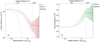 |
Fig. 3 Median radial column density (a) and dust temperature (b) profiles of filament 8. Error bars correspond to the standard deviation of observed values at a given radius. Panel a: red solid line shows the median profile measured in the high-resolution (18.2″) column density map. The background level (at >0.18 pc, ~3 × 1021 cm−2) is marked with a blue-dashed line. The median FWHM of the filament derived from this column density profile is 0.14 ± 0.03 pc. Panel b: dust temperature, which was measured at the center of the filament, is ~ 13 K, comparedto ~15.5 K for the localbackground cloud at >0.18 pc, which is marked by a blue-dashed line. |
3.3 Selection and classification of reliable cores
Dense cores are individual cloud fragments with typical sizes of ≲ 0.1 pc, which correspond to local overdensities and therefore local minima in the gravitational potential of the parent molecular cloud (e.g., Bergin & Tafalla 2007; André et al. 2014). Reliable cores were selected and classified according to the detailed criteria described by Könyves et al. (2015). This method has already been validated and applied to many molecular clouds in the Herschel Gould Belt survey (HGBS – André et al. 2010). The core size was defined as the mean deconvolved FWHM diameter of an equivalent elliptical Gaussian source:
 (5)
(5)
where HL and HS are the major axis and minor axis of the equivalent Gaussian source, and O = 18.2″ is the angular resolution of the column density map. The integrated flux measured for each deblended core at each wavelength by getsources were used to fit an SED with a modified blackbody function, which was also used to create the column density map in Sect. 3.1. The mass, line of sight averaged dust temperature, and peak column density of each core were also estimated. Prestellar cores are gravitationally-bound starless cores that represent fundamental units of star formation (Ward-Thompson et al. 2007; Bergin & Tafalla 2007; André et al. 2014). In a first approximation, the structure of these cores resembles that of self-gravitating isothermal equilibrium Bonnor-Ebert (BE) spheroids (Ebert 1955; Bonnor 1956), which are bounded by the ambient pressure of the parent cloud, as observed in many cases (e.g., Alves et al. 2001; Bacmann et al. 2000; Kirk et al. 2005). The BE model is useful even though real cores are not strictly isothermal (e.g., Galli et al. 2002) and not necessarily in hydrostatic equilibrium either (e.g., Ballesteros-Paredes et al. 2003). This model has been widely used as a template to select prestellar cores in, for example, the HGBS survey (see, e.g., Könyves et al. 2015) and ground-based submillimeter observations (see, e.g., Zhang et al. 2015). In particular, although the critical BE mass,  (maximum mass of an equilibrium isothermal sphere for a given temperature and ambient pressure), differs conceptually from the virial mass, it provides a good approximation to the latter for unmagnetized, thermal cores (see, e.g., Li et al. 2013). The critical BE mass can be expressed as (Bonnor 1956)
 (6)
(6)
where RBE is the BE radius. Here, we used the deconvolved FWHM size measured in the column density map to estimate the core radius. Assuming an ambient cloud temperature of 10 K, the isothermal sound speed cs is ~ 0.19 km s−1. When the ratio  , the starless core was deemed to be self-gravitating and classified as a robust prestellar core. Following Könyves et al. (2015), an empirical size-dependent ratio of
  , where
  and
and  are the beam size (18.2″) of the high-resolution column density map and the core FWHM in this map, respectively, was also considered for selecting additional candidate prestellar cores. A protostellar core is a dense core in which there is at least one protostar in the half-power column density contour. We identified 24 unbound starless cores, 20 robust prestellar cores, 11 additional candidate prestellar cores, and two protostellar cores. The core positions are overlaid on the column density map in Fig. A.1 and the physical parameters of the cores are given in Table A.1. About 45% of the prestellar cores lie in thermally supercritical filaments, ~ 45% in transcritical filaments, while the rest (~10%) of the prestellar cores are observed toward clumpy cloud structures. Unbound starless cores are only observed toward subcritical filamentary structures. The derived core masses range from 0.04 to 5.8 M⊙, with a mean value of 0.8 M⊙. The deconvolved core radii range from 0.02 to 0.12 pc, with a mean value of 0.06 pc.
A remarkable string of five regularly spaced, robust prestellar cores is observed along the crest of filament 8 (see Fig. 6). The mean projected spacing between these five cores (# 29, 30, 32, 34, 33) is ~ 0.17 ± 0.1 pc. (see Fig. 8), and their typical mass is ~0.8 M⊙ (see Table 2). To test whether the quasi-periodic pattern of core spacings observed along filament 8 may also occur for a randomly distributed population of cores, we used the publicly available python code FRAGMENT (Clarke et al. 2019)to construct 10 000 random realizations of five cores that are randomly placed along a 0.98-pc-long filament and to compare the resulting overall distribution of nearest-neighbor separations (NNS) with the observed NNS distribution using a Kolmogovov-Smirnov (K-S) test. The results indicate that there is a very low probability, p ~ 0.001 (equivalent to >3σ in Gaussian statistics), that the observed quasi-periodic pattern may arise from an intrinsically random distribution of cores. This means that the quasi-periodic pattern of cores along filament 8 is highly significant.
Another string of four regularly spaced cores is observed along the crest of filament 10 (see Fig. 7), including two robust prestellar cores (core # 43 and 49) and two protostellar cores (core # 44 and 46). Here, the mean projected core spacing is ~0.13 ± 0.02 pc (see Fig. 8). Based on a K-S test similar to the one described above for filament 8, the probability that the observed quasi-periodic pattern may arise from a random distribution of cores is p ~ 0.008 (equivalent to >2.5σ in Gaussian statistics). Thus, the quasi-periodic pattern of cores along filament 10 is also significant, although not as highly significant as in filament 8.
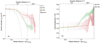 |
Fig. 4 Median radial column density (a) and dust temperature (b) profiles measured on the eastern and western sides of filament 10 (green and red solid lines, respectively). The median FWHM derived from the filament profile in panel a is 0.1 ± 0.03 pc. The column density profile is somewhat wider on the western side, presumably because of the effect of YSO outflows on this filament. The background level, which was measured on the eastern side (at >0.1 pc, ~ 3.5 × 1021 cm−2), is marked with a blue-dashed line. |
Derived physical parameters of the ten selected filaments.
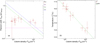 |
Fig. 5 Deconvolved FWHM (Wdec) (panel a) and central dust temperature ( |


3.4 Transverse velocity gradient across filament 8
To investigate the presence of velocity gradients toward filament 8, we selected all SMT 13 CO(2−1) spectra with a signal-to-noise ratio of S∕N > 4. After subtracting a baseline from each spectrum, we fit a Gaussian profile to estimate the centroid velocity at each position and we created a centroid velocity map (see Fig. 9). The average 13 CO(2−1) and 12 CO(2−1) spectra observed with the SMT along the crest of filament 8 are shown in Fig. 10. Based on the centroid velocity map (Fig. 9a), we constructed an average transverse position–velocity plot across filament 8 (Fig. 11). To do so, we selected all 13CO(2−1) spectra observed in a 0.5-pc-wide strip around the filament crest and grouped them in bins of 0.05 pc to calculate a crest-averaged centroid velocity as a function of radial offset from the filament crest (Fig. 11). The average centroid velocity observed along the crest of filament 8 is approximately − 0.36 km s−1. Blue-shifted gas is distributed to the east of the filament crest. The average centroid velocity observed 0.25 pc to the east of the crest is − 0.87 km s−1, corresponding to a relative velocity of approximately − 0.51 km s−1 with respect to the filament. Red-shifted gas is observed to the west of the filament crest. The average velocity observed 0.25 pc to the west of the crest is approximately − 0.21 km s−1, corresponding to a relative velocity of approximately + 0.15 km s−1 with respect to the filament. The best-fit linear velocity gradient is ∇Veast = 2.17 ± 0.27 km s−1 pc−1 on the eastern side and ∇Vwest = 0.74 ± 0.09 km s−1 pc−1 on the western side. There is also a weak longitudinal velocity gradient along the crest of filament 8, from north to south of ~ 0.21 ± 0.03 km s−1 pc−1, which is consistent with the one reported by Imara et al. (2017) on larger scales. We stress, however, that the amplitude of the longitudinal velocity gradient is an order of magnitude lower than the amplitude of the transverse gradient. The observed longitudinal velocity gradient is also a factor of ~2–4 weaker than that measured toward the filaments of the SDC13 infrared dark cloud, which is a hub-filament system (cf. Myers 2009) with a morphology that is very similar to the X-shaped region (Peretto et al. 2014).
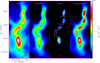 |
Fig. 6 High-resolution (18.2″) column density views of filament 8 and its embedded cores. All maps are shown from 1021 to 2 × 1022 cm−2. Panel a: high-resolution (18.2″) column density map. Panel b: clean-background and core-subtracted filament image that was reconstructed over the full range of spatial scales. The crest of the filament is shown with a blue-dotted line. Panel c: five robust prestellar cores that were identified along this filament (marked by FWHM Gaussian ellipses), which are regularly spaced with measured projected spacings of 0.17, 0.16, 0.15, and 0.18 pc from south to north, respectively. The mean core spacing is 0.17 ± 0.01 pc. Panel d: detected cores overlaid on the filament. |
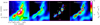 |
Fig. 7 High-resolution (18.2″) column density views of filament 10 and its embedded cores. All maps are shown from 1021 to 3 × 1022 cm−2. Two protostellar cores (core # 44, 46) and two robust prestellar cores (core # 43, 49) are detected along this filament. These four cores are regularly spaced with projectedspacings of 0.11, 0.12, and 0.16 pc, respectively. The average core spacing is 0.13 ± 0.02 pc. |
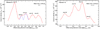 |
Fig. 8 Longitudinal column density profiles of filament 8 (left panel) and filament 10 (right panel). In both cases, the column density profiles (red curves) were obtained from the original high-resolution (18.2″) column density map. Left panel: cores # 32 and 34 partly overlap and they were deblended by getsources using an iterative method. The inferred structure of these two cores is shown by the blue-dashed Gaussian profiles. The four cores in the right panel are clearly separated from one another and they did not require any deblending. |
Derived physical parameters for the cores identified along filaments 8 and 10.
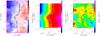 |
Fig. 9 Views of the transverse velocity gradient across filament 8. Panel a: map of centroid velocities observed in 13 CO (2−1), shown from VLSR = −1.86 km s −1 (blue) to VLSR = +1.14 km s −1 (red). The crest of the filament is marked by a black line. The cores identified with getsources are shown by black ellipses, whose sizes correspond to the (major and minor) FWHM diameters of the equivalent Gaussian sources. Panel b: map of the linear transverse-velocity gradient model fitted on the blue-shifted eastern side (2.17 × Xoffset km s−1) and the red-shifted western side (0.74 × Xoffset km s−1) of the filament. Panel c: map of centroid velocities obtained after subtracting the transverse velocity gradient. |
4 Discussion
The Herschel data have revealed the presence of at least two quasi-periodic chains of dense cores (alongfilaments 8 and 10) in the X-shaped region, with a typical projected core spacing of ~ 0.15 pc comparable to, or only ~30–40% higher than, the filament’s inner width in both cases. The length of filament 8 is ~ 1 pc and its line mass is ~ 30 M⊙ pc−1, which is roughly twice the critical line mass (Mline,crit ~ 16 M⊙ pc−1) for an isothermal gas cylinder at 10 K. Filament 10 has about the same mass per unit length, but it is about half the length of filament 8 (see Table 1). In contrast to filament 8 which only includes prestellar cores, filament 10 harbors two embedded protostars and thus may be slightly more evolved, at a somewhat later fragmentation stage. While filament 8 exhibits a pronounced transverse velocity gradient (Sect 3.4 and Fig. 11), there is no clear evidence of such a gradient toward filament 10, but this may be due to confusion of the 12 CO(2−1) data by the outflows from the two embedded protostars. In this section, we discuss the implications of these results for our understanding of fragmentation in star-forming filaments.
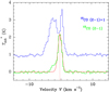 |
Fig. 10 Mean 12CO(2–1) (blue) and 13CO(2–1) (green) spectra observed with the SMT along the crest of filament 8. A
+ 1 K offset was added to the corrected main beam temperature ( |

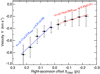 |
Fig. 11 Crest-averaged centroid velocity as a function of the right-ascension offset Xoffset from the crest of filament 8. This shows that the mean transverse velocity gradient observed across filament 8 is ~ 2.17 ± 0.27 km s−1 pc−1 on the eastern, blue-shifted side and ~ 0.74 ± 0.09 km s−1 pc−1 on the western, red-shifted side. |
4.1 Potential evidence of accretion into filament 8
Blue-shifted and red-shifted 12CO(2–1) gas is distributed to the east and to the west of filament 8, respectively, which is a pattern observed up to at least ± 0.4 pc on either side of the filament. This pattern traces a transverse velocity gradient of about 1.5 km s−1 pc−1 on average (see Fig. 9a), which may a priori arise from large-scale accretion, rotation, shearing motions, or a combination of these types of motions. While bulk rotation in most Galactic molecular clouds is known to cause velocity gradients of ≲ 3 km s−1 pc−1 (e.g., Phillips 1999; Braine et al. 2018), it is not likely that the velocity gradient observed here is due to the solid-body rotation of filament 8 around its main axis for the following reasons. First, solid-body rotation would yield the same linear gradient on either side of the filament, which is not the case here (see Fig. 11). Second, the moment of inertia IΔ derived from the (column) density profile of the filament is very large when estimated up to Rmax = 0.4 pc from the filament axis Δ:
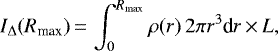
where L is the length of the filament. If the observed velocity gradient is interpreted in terms of rotation at an angular velocity Ω ~ 1.5 km s−1 pc−1 ~ 4.9 × 10⁻¹⁴ rad s−1, this would imply a very high rotational energy per unit length. Accordingly, the ratio of rotational ( ) to gravitational (
 ) energy would also be very high for the rotating filament and cloud system:
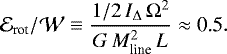
Such a high  ratio is unrealistic because the centrifugal force would then severely distort the filament and result in a (column) density profile, with secondary peaks, that is significantly shallower than the observed profile of Fig. 3a (see Fig. 1 of Recchi et al. 2014 for a normalized angular velocity of
  in the case of filament 8). Shearing motions induced by large-scale interstellar turbulence may lead to the formation of filamentary structures with transverse velocity gradients. In this case, however, the resulting filaments are expected to be non-self-gravitating or subcritical (Hennebelle 2013), which is in contrast to filament 8. Moreover, the dimensionless parameter
  , where ΔV ~ 0.33 km s−1 is half the velocity difference across the filament,is close to 1 here (Cv ~ 0.85), which suggests that the velocity gradient is not due to to the effect of supersonic turbulence, but related to the self-gravity of the filament (Chen et al. 2020).
The most likely interpretation of the transverse velocity gradient is that it results from gravitational accretion motions into filament 8 within a surrounding sheet-like cloud structure. A similar pattern has been reported before for other filament systems, such as Taurus B211/B213 (Palmeirim et al. 2013; Shimajiri et al. 2019b), the Serpens cloud (Fernández-López et al. 2014; Dhabal et al. 2018), and IRDC 18223 (Beuther et al. 2015). Here, the projected velocity gradient observed on the eastern side (2.17 ± 0.27 km s−1 pc−1) is larger than the one on the western side (0.74 ± 0.09 km s−1 pc−1). This is reminiscent of the transverse velocity gradient across the Taurus B211/B213 filament, which is also asymmetric (Palmeirim et al. 2013; Shimajiri et al. 2019b). In the case of the B211/B213 filament, this type of velocity gradient was successfully modeled by Shimajiri et al. (2019b) in terms of gravitational infall of background gas in a parent shell-like structure with different inclination angles to the line of sight on either side of the filament. We suggest that a similar model applies to filament 8 and can estimate the mass accretion rate into the filament as follows.
We define Rout to be the outer radius of the filament, outside of which the (column) density profile (Fig. 3a) starts to fluctuate and to be dominated by the background cloud. From the high-resolution (18.2″) H2 column density map and the radial profile of Fig. 3a, we estimate Rout ~ 0.18 pc and an average background column density of NBackground ~ 3 × 1021 cm−2. The relative velocity of the blue-shifted gas with respect to the line-of-sight velocity at the filament’s center is measured to be  at Rout on the eastern side, while the relative velocity of the red-shifted gas is
  at Rout on the western side. Assuming that the ambient gas is in free-fall motion toward the filament as a result of the gravitational potential of the latter, the free-fall velocity at Rout can be expressed as
  (Palmeirim et al. 2013), where Rinit is the radius where the gas is initially at rest. Here, we estimate Rinit ~ 0.4 pc and Vff ~ 0.32 km s−1 at Rout. The total mass inflow rate from both sides is then expected to be
  . The total mass accretion rate derived from the observed velocities, when ignoring projection effects, is very similar:
  . We conclude that the accretion rate into filament 8 is Ṁline ~ 35–43 M⊙ Myr−1 pc−1, which corresponds to an accretion timescale, Mline∕Ṁline ≈ 0.7 ± 0.2 Myr. Interestingly, the above accretion rate is reminiscent of the rate of 30 M⊙ Myr−1 pc−1 that is found for filaments in hydrodynamic simulations of molecular cloud formation by colliding flows and global hierarchical collapse (Gómez & Vázquez-Semadeni 2014; Vázquez-Semadeni et al. 2019).
4.2 Fragmentation manner of filaments 8 and 10
The presence of two quasi-periodic chains of dense cores in the X-shaped region with a projected spacing similar to the width of the parent filaments is quite remarkable. A few other examples of quasi-periodic configurations of roughly equally spaced dense cores or clumps along filaments have recently been reported in the literature. Using ALMA dust continuum emission at 870 μm, Sánchez-Monge et al. (2014) found regularly spaced condensations with a mean separation of ~ 0.023 pc along the filamentary structure G35.20-0.74N. Jackson et al. (2010) mapped the “Nessie” Nebula, a ~80-pc long filamentary infrared dark cloud (IRDC) in HNC (1–0) emission with the ATNF Mopra Telescope, and they found a characteristic clump spacing of ~4.5 pc (see also Mattern et al. 2018). Tafalla & Hacar (2015) found a quasi-periodic chain of dense cores with a typical inter-core separation of ~ 0.1 pc in the L1495/B213 filament of the Taurus MC (see also Bracco et al. 2017). Wang et al. (2011) found a similar separation of ~ 0.16 pc between dense cores along G28.34+0.06, that is a filamentary IRDC whose line mass is five to eight times larger than the line masses of L1495/B213 and filament 8 here. Shimajiri et al. (2019a) recently reported evidence of two distinct fragmentation modes in the massive NGC 6334 filament (Mline ~ 1000 M⊙ pc−1), with regularly spaced clumps separated by ~0.2–0.3 pc, in turn fragmented into dense cores with a typical spacing of ~0.03–0.1 pc. The above mentioned filaments span a wide range of length scales and line masses and they may not be directly comparable. Nevertheless, it is possible that dense filaments may evolve and fragment in a qualitatively similar manner at low and high line masses (cf. Shimajiri et al. 2019a), and that the same underlying physical mechanism is responsible for their quasi-periodic fragmentation patterns.
Interstellar turbulence is believed to produce a whole spectrum of density fluctuations along filaments, and subcritical filaments are indeed observed to harbor a Kolmogorov-like spectrum of linear density fluctuations (Roy et al. 2015). In the case of thermally transcritical and supercritical filaments, self-gravity can amplify some of these density fluctuations beyond the linear regime, leading to prestellar core formation and protostellar collapse. Linear fragmentation models for the growth of density perturbations along infinitely long, isothermal equilibrium cylinders with Mlin ≈ Mline,crit show that density perturbations with wavelengths greater than ~2 times the filament diameter can grow and predict a characteristic core spacing of ~ 4 × the filament diameter (e.g., Inutsuka & Miyama 1992), or ~5 × the FWHM (e.g., Fischera & Martin 2012). Here, the FWHMdec widths of filaments 8 and 10 are 0.13 ± 0.03 pc and 0.09 ± 0.03 pc, respectively, so we would expect characteristic core spacings of  pc and
  pc in the two filaments according to these models. For these predictions to match the observed (projected) spacings,
  pc and
  pc, the two filaments would have to be seen almost “head-on”, with a viewing angle α of only 15–17° between the filament axis and the line of sight in both cases. Such extreme values of α are quite unlikely, especially for two independent filaments. Assuming random inclinations to the line of sight, the probability of observing a cylindrical filament with a viewing angle of α ≤ α0 is p = 1 −cos α0 or p ~ 6% for α0 = 20°. The probability of observing two filaments (such as filaments 8 and 10 here) with α ≤α0 ≈ 20° in a sample of five transcritical or supercritical filaments (#5, 6, 8, 9, 10 in Table 1) is only
  according to binomial statistics. The null hypothesis that the fragmentation pattern observed in filaments 8 and 10 is consistent with the predictions of classical cylinder fragmentation theory (e.g., Inutsuka & Miyama 1992, 1997) can thus be rejected at the > 2σ confidence level. The typical projected core spacing of ~0.15 pc observed toward filaments 8 and 10 is actually in better agreement with normal or “spherical” Jeans-like fragmentation. In this case,the expected fragmentation lengthscale is the standard Jeans length, which may be expressed as:
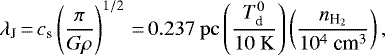 (7)
(7)
where  is the (central) volume density of the filament and cs is the isothermal sound speed. Adopting
  K for the gas temperature and assuming the central densities given in Table 1, the Jeans length λJ is estimated to be 0.11 and 0.15 pc for filament 8 and filament 10, respectively, or 0.13 pc on average. This is very close to the observed value of ~ 0.15 pc.
Several explanations may be proposed to account for the discrepancy between the observed core spacing and the predictions of classical cylinder fragmentation theory. First, filaments 8 and 10 are clearly not perfect, straight cylinders as they exhibit rather pronounced bends along their lengths (cf. Figs. 6 and 7). Using numerical simulations, Gritschneder et al. (2017) investigated the fragmentation properties of filaments including sinusoidal bends or longitudinal oscillations and they show that bending filaments are prone to “geometrical fragmentation”, a process that generates cores at the turning points of the geometrical oscillation, which are separated by half the wavelength of the initial sinusoidal perturbation. This process may be partly at work here. The geometrical deformations observed in filaments 8 and 10 (compared to straight filaments) are not purely sinusoidal, however, and some of the detected cores are apparently not located at clear bends along the filaments (cf. Figs. 6 and 7).
Second, although currently, poorly constrained, magnetic fields may play a key role in controlling the detailed fragmentation manner of molecular filaments (see, e.g., André et al. 2019 for a review), a magnetic field perpendicular to the filament axis tends to increase the wavelength of the most unstable fragmentation mode, that is to say the expected separation between cores, and it may even suppress fragmentation for moderate field strengths (Hanawa et al. 2017). In contrast, a longitudinal magnetic field does not suppress fragmentation and shortens the expected core spacing when expressed in units of the filament diameter (Nakamura et al. 1993; Hanawa et al. 1993). For a strong longitudinal magnetic field (e.g., a plasma  ), the expected core spacing can become comparable to the filament diameter (see Table 1 of Nakamura et al. 1993), as observed here in the case of filaments 8 and 10. The required longitudinal field strength ~ 100 μG at densities ~2–4 × 104cm−3 in the center of filaments 8 and 10 is high, but not unrealistic in view of existing Zeeman measurements in MCs (Crutcher 2012). Observationally, the large-scale magnetic field tends to be perpendicular to thermally transcritical or supercritical filaments, such as filaments 8 and 10 (Planck Collaboration Int. XXXII 2016; Planck Collaboration Int. XXXV 2016). However, little is known about the geometry of the field in the interior of such filaments. There is a hint from Planck polarization data that the magnetic field direction may change in some cases from nearly perpendicular in the parent cloud to more parallel within the filament (Planck Collaboration Int. XXXIII 2016), but higher-resolution data would be needed to be truly conclusive. In particular, more work would be required to assess the magnetic field topology within filaments 8 and 10 and to clarify whether magnetic fields may account for the observed fragmentation lengthscale.
Third, neither filament 8 nor filament 10 is an isolated cloud structure in perfect hydrostatic equilibrium. As discussed in Sect. 4.1, the transverse velocity gradient seen across filament 8 (Sect. 3.4 and Fig. 11) provides evidence that the filament is in the process of accreting gas from the ambient cloud (cf. Chen & Ostriker 2014; Shimajiri et al. 2019b). As is shown by Clarke et al. (2016), the presence of accretion modifies the process of filament fragmentation. Indeed, Clarke et al. (2016) show that the fastest growing mode for density perturbations in a nearly critical, accreting filament moves to shorter wavelengths, and it can thus become significantly shorter than ~ 4 × the filament width when the accretion rate  that the filament experienced during its formation (up to the point at which it became critical) exceeds Σfil cs∕2. The latter essentially means that the filament formed dynamically as opposed to quasi-statically via subsonic assembling motions. In the case of filament 8, the present accretion rate was estimated to be Ṁline = 40 ± 10 M⊙ pc−1 Myr−1 in Sect. 4.1 while Σfil cs∕2 is ~ 20 M⊙ pc−1 Myr−1. It is thus plausible that filament 8 formed dynamically on a relatively short timescale, which may explain the quasi-periodic spacing of its cores on a scale comparable to its width.
5 Conclusions
We performed a detailed study of filaments and cores in the X-shaped nebula of the California MC using a high-resolution (18.2″) column density map constructed from Herschel data, along with 12CO(2−1) and 13CO(2−1) data from the SMT 10 m telescope. Our main findings can be summarized as follows.
- 1.
We selected ten robust filaments with aspect ratios of AR > 4 and column density contrasts of C > 0.5 from a skeleton network obtained with the getfilaments algorithm. The dust temperatures of the filaments are anti-correlated with their column densities (
 ). The deconvolved FWHM (Wdec) of the ten filaments range from 0.09 to 0.18 pc and are uncorrelated with their column densities (
 ). The derived median filament width, 0.12 ± 0.03 pc, is consistent with the common inner width of ~0.1 pc, which was measured by Arzoumanian et al. (2011, 2019) for Herschel filaments in nearby molecular clouds.
 - 2.
We identified two thermally supercritical filaments: filaments 8 and 10, which both exhibit quasi-periodic chains of dense cores. The typical projected core spacing is ~0.15 pc, which is close or only ~30–40% higher than the filament inner width. Five prestellar cores form the chain structure of filament 8. There is a transverse velocity gradient across filament 8, suggesting that this filament is accreting gas from the surrounding ambient gas reservoir with an accretion rate of Ṁ ~ 40 ± 10 M⊙ Myr−1 pc−1. Filament 10 is ~0.5 pc away from filament 8 and at a later fragmentation stage than filament 8. Two prestellar cores and two protostellar cores form the chain structure of this filament.
- 3.
We emphasize that classical cylinder fragmentation theory cannot account for the observed fragmentation properties of filaments 8 and 10. We suggest that three key factors may explain why the observed core spacing is shorter than the standard fragmentation lengthscale of equilibrium filaments. First, filaments 8 and 10 are not straight cylinder structures and they feature bends along their crests which likely affect the fragmentation process. Second, if a longitudinal magnetic field of ~100 μG is present at the center of filaments 8 and 10, the characteristic fragmentation lengthscale may become comparable to the filament diameter as observed. Third, at least in the case of filament 8, the presence of external accretion from the ambient cloud may enhance initial density perturbations, leading to a shorter core spacing compared to an isolated filament.
To conclude, our work suggests that the coupling of star-forming filaments with their parent clouds plays a critical role for their detailed fragmentation properties, due for instance to gravitational accretion of ambient gas or external compression of a pre-existing longitudinal magnetic field. Comprehensive observational studies similar to the one presented here would be desirable to confirm the generality of this conclusion. Polarimetric observations at similar resolution to the present study will also be necessary to clarify whether the magnetic field has the required geometry and strength to play a significant role.
Acknowledgements
We would like to thank the anonymous referee for valuable comments which improved the quality of the paper. The SMT data presented in this paper are based on the ESO-ARO programme ID 196.C-0999(A). This work was carried out in the HGBS group of the Astrophysics Department (DAp/AIM) at CEA Paris-Saclay. G.Z. acknowledges support from a Chinese Government Scholarship (No. 201804910583). We also acknowledge support from the French national programs of CNRS/INSU on stellar and ISM physics (PNPS and PCMI). K.W. acknowledges support by the National Key Research and Development Program of China (2017YFA0402702, 2019YFA0405100), the National Science Foundation of China (11973013, 11721303), and a starting grant at the Kavli Institute for Astronomy and Astrophysics, Peking University (7101502287).
Appendix A Core location distribution
Physical parameters of the cores identified with Herschel in the X-shaped nebula region.
 |
Fig. A.1 Positions of the 57 dense cores (FWHM Gaussian ellipses) identified in the X-shaped nebula region overlaid on the Herschel high-resolution (18.2″) column density map. Magenta ellipses, blue ellipses, black ellipses, and green stars mark the 24 unbound starless cores, the 11 candidate prestellar cores, the 20 robust prestellar cores, and the two protostellar cores, respectively (see Sect. 3.3). The skeleton of the filament network extracted in Sect. 3.2 is shown by white curves. The thirteen 5′ × 5′ fields covered by the SMT CO observations are marked as black boxes. |
References
- Alves, J. F., Lada, C. J., & Lada, E. A. 2001, Nature, 409, 159 [NASA ADS] [CrossRef] [PubMed] [Google Scholar]
- André, P. 2017, CR Geosci., 349, 187 [Google Scholar]
- André, P., Men’shchikov, A., Bontemps, S., et al. 2010, A&A, 518, L102 [NASA ADS] [CrossRef] [EDP Sciences] [Google Scholar]
- André, P., Di Francesco, J., Ward-Thompson, D., et al. 2014, Protostars and Planets VI, eds. H. Beuther, R. S. Klessen, C. P. Dullemond, & T. Henning (Tucson, AZ: University of Arizona Press), 27 [Google Scholar]
- André, P., Hughes, A., Guillet, V., et al. 2019, PASA, 36, e029 [CrossRef] [Google Scholar]
- Andrews, S. M., & Wolk, S. J. 2008, Handbook of Star Forming Regions, Volume I: The Northern Sky, ed. B. Reipurth (San Francisci: ASP Monograph Publications), 390 [Google Scholar]
- Arzoumanian, D., André, P., Didelon, P., et al. 2011, A&A, 529, L6 [Google Scholar]
- Arzoumanian, D., André, P., Könyves, V., et al. 2019, A&A, 621, A42 [NASA ADS] [CrossRef] [EDP Sciences] [Google Scholar]
- Bacmann, A., André, P., Puget, J. L., et al. 2000, A&A, 361, 555 [Google Scholar]
- Ballesteros-Paredes, J., Klessen, R. S., & Vázquez-Semadeni, E. 2003, ApJ, 592, 188 [NASA ADS] [CrossRef] [Google Scholar]
- Bergin, E. A., & Tafalla, M. 2007, ARA&A, 45, 339 [NASA ADS] [CrossRef] [Google Scholar]
- Bernard, J. P., Paradis, D., Marshall, D. J., et al. 2010, A&A, 518, L88 [NASA ADS] [CrossRef] [EDP Sciences] [Google Scholar]
- Beuther, H., Ragan, S. E., Johnston, K., et al. 2015, A&A, 584, A67 [NASA ADS] [CrossRef] [EDP Sciences] [Google Scholar]
- Bonnor, W. B. 1956, MNRAS, 116, 351 [CrossRef] [Google Scholar]
- Bracco, A., Palmeirim, P., André, P., et al. 2017, A&A, 604, A52 [NASA ADS] [CrossRef] [EDP Sciences] [Google Scholar]
- Braine, J., Rosolowsky, E., Gratier, P., Corbelli, E., & Schuster, K. F. 2018, A&A, 612, A51 [NASA ADS] [CrossRef] [EDP Sciences] [Google Scholar]
- Broekhoven-Fiene, H., Matthews, B. C., Harvey, P. M., et al. 2014, ApJ, 786, 37 [NASA ADS] [CrossRef] [Google Scholar]
- Chambers, K. C., Magnier, E. A., Metcalfe, N., et al. 2016, ArXiv e-prints [arXiv:1612.05560] [Google Scholar]
- Chen, C.-Y., & Ostriker, E. C. 2014, ApJ, 785, 69 [NASA ADS] [CrossRef] [Google Scholar]
- Chen, C.-Y., Mundy, L. G., Ostriker, E. C., Storm, S., & Dhabal, A. 2020, MNRAS, 494, 3675 [CrossRef] [Google Scholar]
- Clarke, S. D., Whitworth, A. P., & Hubber, D. A. 2016, MNRAS, 458, 319 [NASA ADS] [CrossRef] [Google Scholar]
- Clarke, S. D., Williams, G. M., Ibáñez-Mejía, J. C., & Walch, S. 2019, MNRAS, 484, 4024 [NASA ADS] [CrossRef] [Google Scholar]
- Crutcher, R. M. 2012, ARA&A, 50, 29 [NASA ADS] [CrossRef] [Google Scholar]
- Dhabal, A., Mundy, L. G., Rizzo, M. J., Storm, S., & Teuben, P. 2018, ApJ, 853, 169 [NASA ADS] [CrossRef] [Google Scholar]
- Ebert, R. 1955, ZAp, 37, 217 [Google Scholar]
- Evans, Neal J., I. 1991, ASP Conf. Ser., 20, 45 [Google Scholar]
- Federrath, C. 2016, MNRAS, 457, 375 [NASA ADS] [CrossRef] [Google Scholar]
- Fernández-López, M., Arce, H. G., Looney, L., et al. 2014, ApJ, 790, L19 [NASA ADS] [CrossRef] [Google Scholar]
- Fischera, J., & Martin, P. G. 2012, A&A, 542, A77 [NASA ADS] [CrossRef] [EDP Sciences] [Google Scholar]
- Gaia Collaboration (Brown, A. G. A., et al.) 2018, A&A, 616, A1 [NASA ADS] [CrossRef] [EDP Sciences] [Google Scholar]
- Galli, D., Walmsley, M., & Gonçalves, J. 2002, A&A, 394, 275 [NASA ADS] [CrossRef] [EDP Sciences] [Google Scholar]
- Gómez, G. C., & Vázquez-Semadeni, E. 2014, ApJ, 791, 124 [NASA ADS] [CrossRef] [Google Scholar]
- Griffin, M. J., Abergel, A., Abreu, A., et al. 2010, A&A, 518, L3 [Google Scholar]
- Gritschneder, M., Heigl, S., & Burkert, A. 2017, ApJ, 834, 202 [NASA ADS] [CrossRef] [Google Scholar]
- Großschedl, J. E., Alves, J., Teixeira, P. S., et al. 2019, A&A, 622, A149 [NASA ADS] [CrossRef] [EDP Sciences] [Google Scholar]
- Hanawa, T., Nakamura, F., Matsumoto, T., et al. 1993, ApJ, 404, L83 [NASA ADS] [CrossRef] [Google Scholar]
- Hanawa, T., Kudoh, T., & Tomisaka, K. 2017, ApJ, 848, 2 [CrossRef] [Google Scholar]
- Harvey, P. M., Fallscheer, C., Ginsburg, A., et al. 2013, ApJ, 764, 133 [NASA ADS] [CrossRef] [Google Scholar]
- Hennebelle, P. 2013, A&A, 556, A153 [NASA ADS] [CrossRef] [EDP Sciences] [Google Scholar]
- Imara, N., Lada, C., Lewis, J., et al. 2017, ApJ, 840, 119 [CrossRef] [Google Scholar]
- Inutsuka, S.-I., & Miyama, S. M. 1992, ApJ, 388, 392 [NASA ADS] [CrossRef] [Google Scholar]
- Inutsuka, S.-i.,& Miyama, S. M. 1997, ApJ, 480, 681 [NASA ADS] [CrossRef] [Google Scholar]
- Jackson, J. M., Finn, S. C., Chambers, E. T., Rathborne, J. M., & Simon, R. 2010, ApJ, 719, L185 [NASA ADS] [CrossRef] [Google Scholar]
- Kainulainen, J., Ragan, S. E., Henning, T., & Stutz, A. 2013, A&A, 557, A120 [NASA ADS] [CrossRef] [EDP Sciences] [Google Scholar]
- Kainulainen, J., Stutz, A. M., Stanke, T., et al. 2017, A&A, 600, A141 [NASA ADS] [CrossRef] [EDP Sciences] [Google Scholar]
- Kirk, J. M., Ward-Thompson, D., & André, P. 2005, MNRAS, 360, 1506 [NASA ADS] [CrossRef] [Google Scholar]
- Kirk, H., Myers, P. C., Bourke, T. L., et al. 2013, ApJ, 766, 115 [NASA ADS] [CrossRef] [Google Scholar]
- Könyves, V., André, P., Men’shchikov, A., et al. 2015, A&A, 584, A91 [NASA ADS] [CrossRef] [EDP Sciences] [Google Scholar]
- Könyves, V., André, P., Arzoumanian, D., et al. 2020, A&A, 635, A34 [CrossRef] [EDP Sciences] [Google Scholar]
- Lada, C. J., Lombardi, M., & Alves, J. F. 2009, ApJ, 703, 52 [NASA ADS] [CrossRef] [Google Scholar]
- Lada, C. J., Lewis, J. A., Lombardi, M., & Alves, J. 2017, A&A, 606, A100 [NASA ADS] [CrossRef] [EDP Sciences] [Google Scholar]
- Ladjelate, B., André, P., Könyves, V., et al. 2020, A&A, 638, A74 [CrossRef] [EDP Sciences] [Google Scholar]
- Li, D., Kauffmann, J., Zhang, Q., & Chen, W. 2013, ApJ, 768, L5 [NASA ADS] [CrossRef] [Google Scholar]
- Mattern, M., Kainulainen, J., Zhang, M., & Beuther, H. 2018, A&A, 616, A78 [NASA ADS] [CrossRef] [EDP Sciences] [Google Scholar]
- Men’shchikov, A. 2013, A&A, 560, A63 [NASA ADS] [CrossRef] [EDP Sciences] [Google Scholar]
- Men’shchikov, A. 2016, A&A, 593, A71 [NASA ADS] [CrossRef] [EDP Sciences] [Google Scholar]
- Men’shchikov, A. 2017, A&A, 607, A64 [NASA ADS] [CrossRef] [EDP Sciences] [Google Scholar]
- Men’shchikov, A., André, P., Didelon, P., et al. 2010, A&A, 518, L103 [NASA ADS] [CrossRef] [EDP Sciences] [Google Scholar]
- Men’shchikov, A., André, P., Didelon, P., et al. 2012, A&A, 542, A81 [NASA ADS] [CrossRef] [EDP Sciences] [Google Scholar]
- Myers, P. C. 2009, ApJ, 700, 1609 [NASA ADS] [CrossRef] [EDP Sciences] [Google Scholar]
- Nakamura, F., Hanawa, T., & Nakano, T. 1993, PASJ, 45, 551 [NASA ADS] [Google Scholar]
- Ostriker, J. 1964, ApJ, 140, 1056 [NASA ADS] [CrossRef] [MathSciNet] [Google Scholar]
- Palmeirim, P., André, P., Kirk, J., et al. 2013, A&A, 550, A38 [NASA ADS] [CrossRef] [EDP Sciences] [Google Scholar]
- Peretto, N., Fuller, G. A., André, P., et al. 2014, A&A, 561, A83 [NASA ADS] [CrossRef] [EDP Sciences] [Google Scholar]
- Phillips, J. P. 1999, A&AS, 134, 241 [NASA ADS] [CrossRef] [EDP Sciences] [Google Scholar]
- Planck Collaboration Int XXXII. 2016, A&A, 586, A135 [NASA ADS] [CrossRef] [EDP Sciences] [Google Scholar]
- Planck Collaboration Int XXXIII. 2016, A&A, 586, A136 [NASA ADS] [CrossRef] [EDP Sciences] [Google Scholar]
- Planck Collaboration Int XXXV. 2016, A&A, 586, A138 [NASA ADS] [CrossRef] [EDP Sciences] [Google Scholar]
- Poglitsch, A., Waelkens, C., Geis, N., et al. 2010, A&A, 518, L2 [NASA ADS] [CrossRef] [EDP Sciences] [Google Scholar]
- Pudritz, R. E., & Kevlahan, N. K. R. 2013, Phil. Trans. R. Soc. London, Ser. A, 371, 20120248 [Google Scholar]
- Recchi, S., Hacar, A., & Palestini, A. 2014, MNRAS, 444, 1775 [NASA ADS] [CrossRef] [Google Scholar]
- Roy, A., André, P., Palmeirim, P., et al. 2014, A&A, 562, A138 [NASA ADS] [CrossRef] [EDP Sciences] [Google Scholar]
- Roy, A., André, P., Arzoumanian, D., et al. 2015, A&A, 584, A111 [NASA ADS] [CrossRef] [EDP Sciences] [Google Scholar]
- Sánchez-Monge, Á., Beltrán, M. T., Cesaroni, R., et al. 2014, A&A, 569, A11 [NASA ADS] [CrossRef] [EDP Sciences] [Google Scholar]
- Schlafly, E. F., Green, G., Finkbeiner, D. P., et al. 2014, ApJ, 786, 29 [NASA ADS] [CrossRef] [Google Scholar]
- Shimajiri, Y., André, P., Ntormousi, E., et al. 2019a, A&A, 632, A83 [NASA ADS] [CrossRef] [EDP Sciences] [Google Scholar]
- Shimajiri, Y., André, P., Palmeirim, P., et al. 2019b, A&A, 623, A16 [NASA ADS] [CrossRef] [EDP Sciences] [Google Scholar]
- Tafalla, M., & Hacar, A. 2015, A&A, 574, A104 [NASA ADS] [CrossRef] [EDP Sciences] [Google Scholar]
- Vázquez-Semadeni, E., Palau, A., Ballesteros-Paredes, J., Gómez, G. C., & Zamora-Avilés, M. 2019, MNRAS, 490, 3061 [NASA ADS] [CrossRef] [Google Scholar]
- Wang, K., Zhang, Q., Wu, Y., & Zhang, H. 2011, ApJ, 735, 64 [NASA ADS] [CrossRef] [Google Scholar]
- Wang, K., Testi, L., Ginsburg, A., et al. 2015, MNRAS, 450, 4043 [NASA ADS] [CrossRef] [MathSciNet] [Google Scholar]
- Wang, K., Zahorecz, S., Cunningham, M. R., et al. 2018, Res. Notes Amer. Astron. Soc., 2, 2 [NASA ADS] [CrossRef] [Google Scholar]
- Ward-Thompson, D., André, P., Crutcher, R., et al. 2007, in Protostars and Planets V, eds. B. Reipurth, D. Jewitt, & K. Keil (Tucson, AZ: University of Arizona Press), 33 [Google Scholar]
- Yan, Q.-Z., Zhang, B., Xu, Y., et al. 2019, A&A, 624, A6 [NASA ADS] [CrossRef] [EDP Sciences] [Google Scholar]
- Zhang, G., Li, D., Hyde, A. K., et al. 2015, Sci. China Phys. Mech. Astron., 58, 5561 [Google Scholar]
- Zhang, G.-Y., Xu, J.-L., Vasyunin, A. I., et al. 2018, A&A, 620, A163 [CrossRef] [EDP Sciences] [Google Scholar]
- Zucker, C., Speagle, J. S., Schlafly, E. F., et al. 2019, ApJ, 879, 125 [NASA ADS] [CrossRef] [Google Scholar]
Version 2.190425 of getsources was used here.
All Tables
Physical parameters of the cores identified with Herschel in the X-shaped nebula region.
All Figures
|
Fig. 1 Large-scale column density map of the California MC derived from Planck 850 μm optical-depth data (5′ resolution). The location of the X-shaped nebula region is marked with a black square. |
| In the text | |
|
Fig. 2 Blow-up column density views of the X-shaped nebula region in the California MC. Panel A: filtered version of the high-resolution (18.2″) column density map, showing partially-reconstructed filaments with transverse angular scales only up to ~ 100″ from getfilaments (cf. Sect. 2.4.3 in Men’shchikov 2013). The background image shows field stars from the Pan-STARRS optical survey (Chambers et al. 2016). Panel B: unfiltered high-resolution column density map with the network of filamentary structures identified by getfilaments overlaid in white. The crests of the ten filaments selected in Sect. 3.2 are highlighted in black and magenta for thermally supercritical filaments with Mline >Mline,crit and subcritical filaments with Mline < Mline,crit, respectively. |
| In the text | |
|
Fig. 3 Median radial column density (a) and dust temperature (b) profiles of filament 8. Error bars correspond to the standard deviation of observed values at a given radius. Panel a: red solid line shows the median profile measured in the high-resolution (18.2″) column density map. The background level (at >0.18 pc, ~3 × 1021 cm−2) is marked with a blue-dashed line. The median FWHM of the filament derived from this column density profile is 0.14 ± 0.03 pc. Panel b: dust temperature, which was measured at the center of the filament, is ~ 13 K, comparedto ~15.5 K for the localbackground cloud at >0.18 pc, which is marked by a blue-dashed line. |
| In the text | |
|
Fig. 4 Median radial column density (a) and dust temperature (b) profiles measured on the eastern and western sides of filament 10 (green and red solid lines, respectively). The median FWHM derived from the filament profile in panel a is 0.1 ± 0.03 pc. The column density profile is somewhat wider on the western side, presumably because of the effect of YSO outflows on this filament. The background level, which was measured on the eastern side (at >0.1 pc, ~ 3.5 × 1021 cm−2), is marked with a blue-dashed line. |
| In the text | |
|
Fig. 5 Deconvolved FWHM (Wdec) (panel a) and central dust temperature ( |
| In the text | |
|
Fig. 6 High-resolution (18.2″) column density views of filament 8 and its embedded cores. All maps are shown from 1021 to 2 × 1022 cm−2. Panel a: high-resolution (18.2″) column density map. Panel b: clean-background and core-subtracted filament image that was reconstructed over the full range of spatial scales. The crest of the filament is shown with a blue-dotted line. Panel c: five robust prestellar cores that were identified along this filament (marked by FWHM Gaussian ellipses), which are regularly spaced with measured projected spacings of 0.17, 0.16, 0.15, and 0.18 pc from south to north, respectively. The mean core spacing is 0.17 ± 0.01 pc. Panel d: detected cores overlaid on the filament. |
| In the text | |
|
Fig. 7 High-resolution (18.2″) column density views of filament 10 and its embedded cores. All maps are shown from 1021 to 3 × 1022 cm−2. Two protostellar cores (core # 44, 46) and two robust prestellar cores (core # 43, 49) are detected along this filament. These four cores are regularly spaced with projectedspacings of 0.11, 0.12, and 0.16 pc, respectively. The average core spacing is 0.13 ± 0.02 pc. |
| In the text | |
|
Fig. 8 Longitudinal column density profiles of filament 8 (left panel) and filament 10 (right panel). In both cases, the column density profiles (red curves) were obtained from the original high-resolution (18.2″) column density map. Left panel: cores # 32 and 34 partly overlap and they were deblended by getsources using an iterative method. The inferred structure of these two cores is shown by the blue-dashed Gaussian profiles. The four cores in the right panel are clearly separated from one another and they did not require any deblending. |
| In the text | |
|
Fig. 9 Views of the transverse velocity gradient across filament 8. Panel a: map of centroid velocities observed in 13 CO (2−1), shown from VLSR = −1.86 km s −1 (blue) to VLSR = +1.14 km s −1 (red). The crest of the filament is marked by a black line. The cores identified with getsources are shown by black ellipses, whose sizes correspond to the (major and minor) FWHM diameters of the equivalent Gaussian sources. Panel b: map of the linear transverse-velocity gradient model fitted on the blue-shifted eastern side (2.17 × Xoffset km s−1) and the red-shifted western side (0.74 × Xoffset km s−1) of the filament. Panel c: map of centroid velocities obtained after subtracting the transverse velocity gradient. |
| In the text | |
|
Fig. 10 Mean 12CO(2–1) (blue) and 13CO(2–1) (green) spectra observed with the SMT along the crest of filament 8. A
+ 1 K offset was added to the corrected main beam temperature ( |
| In the text | |
|
Fig. 11 Crest-averaged centroid velocity as a function of the right-ascension offset Xoffset from the crest of filament 8. This shows that the mean transverse velocity gradient observed across filament 8 is ~ 2.17 ± 0.27 km s−1 pc−1 on the eastern, blue-shifted side and ~ 0.74 ± 0.09 km s−1 pc−1 on the western, red-shifted side. |
| In the text | |
|
Fig. A.1 Positions of the 57 dense cores (FWHM Gaussian ellipses) identified in the X-shaped nebula region overlaid on the Herschel high-resolution (18.2″) column density map. Magenta ellipses, blue ellipses, black ellipses, and green stars mark the 24 unbound starless cores, the 11 candidate prestellar cores, the 20 robust prestellar cores, and the two protostellar cores, respectively (see Sect. 3.3). The skeleton of the filament network extracted in Sect. 3.2 is shown by white curves. The thirteen 5′ × 5′ fields covered by the SMT CO observations are marked as black boxes. |
| In the text | |
Current usage metrics show cumulative count of Article Views (full-text article views including HTML views, PDF and ePub downloads, according to the available data) and Abstracts Views on Vision4Press platform.
Data correspond to usage on the plateform after 2015. The current usage metrics is available 48-96 hours after online publication and is updated daily on week days.
Initial download of the metrics may take a while.