| Issue |
A&A
Volume 646, February 2021
|
|
|---|---|---|
| Article Number | A68 | |
| Number of page(s) | 15 | |
| Section | Extragalactic astronomy | |
| DOI | https://doi.org/10.1051/0004-6361/201936460 | |
| Published online | 09 February 2021 | |
A low [CII]/[NII] ratio in the center of a massive galaxy at z = 3.7: Evidence for a transition to quiescence at high redshift?
1
Astrophysics, Department of Physics, Keble Road, Oxford OX1 3RH, UK
e-mail: cschreib@orange.fr
2
Centre for Astrophysics and Supercomputing, Swinburne University of Technology, Hawthorn, VIC 3122, Australia
3
George P. and Cynthia W. Mitchell Institute for Fundamental Physics and Astronomy, Department of Physics and Astronomy, Texas A&M University, College Station, TX 77843, USA
4
Núcleo de Astronomía, Facultad de Ingeniería y Ciencias, Universidad Diego Portales, Ejército Libertador 441, Santiago 8320000, Chile
5
AIM-Paris-Saclay, CEA/DSM/Irfu – CNRS – Université Paris Diderot, CEA-Saclay, Pt Courrier 131, 91191 Gif-sur-Yvette, France
6
Leiden Observatory, Leiden University, 2300 RA Leiden, The Netherlands
7
Department of Astronomy, University of Geneva, 51 Ch. des Maillettes, 1290 Versoix, Switzerland
8
Faculty of Physics, Ludwig-Maximilians Universität, Scheinerstr. 1, 81679 Munich, Germany
9
Research Centre for Astronomy, Astrophysics & Astrophotonics, Macquarie University, Sydney, NSW 2109, Australia
10
Department of Physics & Astronomy, Macquarie University, Sydney, NSW 2109, Australia
11
Max-Planck Institut für Astronomie, Königstuhl 17, 69117 Heidelberg, Germany
12
Australia Telescope National Facility, CSIRO Astronomy and Space Science, PO Box 76 Epping, NSW 1710, Australia
13
School of Physics, University of New South Wales, Sydney, NSW 2052, Australia
14
Institute of Astronomy, The University of Tokyo, Osawa, Mitaka, Tokyo 181-0015, Japan
15
National Astronomical Observatory of Japan, Mitaka, Tokyo 181-8588, Japan
16
Chinese Academy of Sciences South America Center for Astronomy (CASSACA), National Astronomical Observatories, CAS, Beijing 100101, PR China
17
Institute of Astrophysics, Foundation for Research and Technology–Hellas (FORTH), Heraklion 70013, Greece
Received:
5
August
2019
Accepted:
26
November
2020
Understanding the process of quenching is one of the major open questions in galaxy evolution and crucial insights may be obtained by studying quenched galaxies at high redshifts at epochs when the Universe and the galaxies were younger and simpler to model. However, establishing the degree of quiescence in high-redshift galaxies is a challenging task. One notable example is Hyde, a recently discovered galaxy at zspec = 3.709. Equally as compact (r1/2 ∼ 0.5 kpc) and massive (M* ∼ 1011 M⊙) as its quenched neighbor Jekyll, it is also extremely obscured yet only moderately luminous in the sub-millimeter. Panchromatic modeling has suggested it could be the first galaxy found in transition to quenching at z > 3, however, the data are also consistent with a broad range of star-formation activity, from fully quenched to moderate star-formation rates (SFR) in the lower scatter of the galaxy main-sequence. Here, we describe Atacama Large Millimeter Array observations of the [C II] 157 μm and [N II] 205 μm far-infrared emission lines. The [C II] emission within the half-light radius is dominated by ionized gas, while the outskirts are dominated by photo-dissociation regions or neutral gas. This suggests that the ionization in the center is not primarily powered by ongoing star formation, and is instead coming from remnant stellar populations formed in an older burst or from a moderate active galactic nucleus . Accounting for this information in the multi-wavelength modeling provides a tighter constraint on the star formation rate of SFR = 50−18+24 M⊙ yr−1 yr−1. This rules out fully quenched solutions and favors SFRs more than factor of two lower than expected for a main-sequence galaxy, confirming the nature of Hyde as a transition galaxy. These results suggest that quenching happens from inside-out and starts before the galaxy expels or consumes all its gas reservoirs. Similar observations of a sample of massive and obscured galaxies would determine whether this is an isolated case or the norm for quenching at high redshift.
Key words: galaxies: evolution / galaxies: high-redshift / galaxies: star formation / submillimeter: galaxies
Note to the reader: The title of the article was corrected on 16 June 2021. A question mark was missing at the end. A corrigendum has also been published here.
© ESO 2021
1. Introduction
Massive galaxies in the low-redshift Universe are observed to be mostly quiescent, with current star formation rates lower than 1% of their past average (e.g., Pasquali et al. 2006). But the way in which galaxies quench their star formation and turn into massive, red early-type galaxies is one of the key unresolved questions of galaxy evolution.
While a number of mechanisms have been proposed in the literature to explain what causes galaxies to stop, reduce, or prevent star formation – including black hole feedback, strong outflows, or gas stripping (e.g., Silk & Rees 1998; Birnboim & Dekel 2003; Croton et al. 2006; Gabor & Davé 2012; Martig et al. 2009; Förster Schreiber et al. 2014; Genzel et al. 2014; Peng et al. 2015), it is still not known which of these mechanisms is most important in explaining the emergence of quenched galaxies. Crucial insight can be gained by studying quiescent galaxies at higher redshift, where the available time for feedback processes to act is shorter, limiting the range of possible mechanisms. Recent works have shown that massive quiescent galaxies had already existed as early as z = 4 (e.g., Labbé et al. 2005; Kriek et al. 2009; Gobat et al. 2012; Merlin et al. 2018; Schreiber et al. 2018a; Belli et al. 2019) at an epoch where state-of-the-art numerical simulations predict that all galaxies would have been forming stars (e.g., Wellons et al. 2015; Davé et al. 2016). These galaxies must have had massive star-forming progenitors at even higher redshifts, and because the age of the Universe was then comparable to their estimated stellar ages (on the order of a billion years or less), they must have quenched shortly before being observed. The main actor in this abrupt quiescence may therefore be easier to identify than in lower-redshift objects, which are seen after several billion years of passive evolution.
An interesting case is that of the most distant known quiescent galaxy to date, at zspec = 3.715 (Glazebrook et al. 2017). The detection of sub-millimeter emission toward this object (Simpson et al. 2017) was later found to arise from a nearby, extremely obscured galaxy at the same redshift (Schreiber et al. 2018b, hereafter S18). This was demonstrated via an ALMA detection of the [C II] line blueshifted by 550 km s−1 as compared to the Balmer absorption lines of the quiescent galaxy and most convincingly by the improved spatial resolution (0.4″) and depth of the sub-millimeter imaging, showing that both the [C II] and dust emissions are produced by a separate, rotating galaxy that is mostly unresolved (0.1″ radius) and located 0.5″ away from the quiescent galaxy. The pair was dubbed “Jekyll and Hyde”, with Jekyll being the quiescent galaxy and Hyde the obscured galaxy.
In S18, we performed an extensive analysis of the rich multi-wavelength data at hand to understand the physical conditions in the obscured galaxy known as Hyde. We showed that despite its extreme obscuration and sub-mm detection, this galaxy appears to form stars at a relatively slow pace, with a star-formation rate of SFR < 100 M⊙ yr−1 and a stellar mass of M* ≃ 1011 M⊙. Given the strong obscuration (AV ≃ 3) and the galaxy’s large stellar mass, the infrared luminosity is, in fact, low enough (LIR ≃ 1012 L⊙) that it may be entirely powered by intermediate-age stars, such that its current SFR (averaged over the last 10 Myr) could be as low as zero. Although these data are also consistent with Hyde being simply a normal galaxy in the lower envelope of the main sequence, the possibility of it being quenched or in transition to quenching is particularly interesting. Indeed, given that this galaxy is still obscured and is therefore likely to contain substantial gas reservoirs, this would be at odds with a number of proposed quenching mechanisms that require full removal or consumption of the gas reservoirs prior to quenching.
This surprising conclusion is nevertheless independently supported by a number of pieces of evidence, first reported in S18 and summarized here for convenience: (a) its dust temperature (Tdust ≃ 30 K) is almost 10 K lower than the average for z ∼ 4 galaxies (Schreiber et al. 2018c), which suggests a softer-than-average radiation field; (b) its compact dust continuum size of about 0.5 kpc is smaller than the rest-ultraviolet size of all z ∼ 4 star-forming galaxies in the same field and is, instead, similar to that of quiescent galaxies (Straatman et al. 2015); and (c) its L[C II]/LFIR ratio is abnormally low for a galaxy of this luminosity, which we showed could be explained by a recent truncation of star formation, although other explanations for the observed [C II] deficit could not be excluded. Considered independently, none of these facts is conclusive or extremely unusual, and indeed there are other examples of galaxies which share at least one of these properties (e.g., similar compactness, dust temperature, or L[C II]/LFIR ratio). It is, however, the sum of these facts which suggests an abnormal process is at play in this galaxy; to our knowledge, such a combination of observables is unique among distant massive galaxies. Although all these signs may point towards a case of Hyde being caught in a very specific phase, possibly in transition to quiescence, none of the data available at the time allowed us to prove this conclusively. In light of the results presented in this paper, we describe these points further on in our discussion.
In this paper, we exploit new spectroscopic data from the Atacama Large Millimeter Array (ALMA) to address this question, combining observations of the [C II] and [N II] (205.178 μm) emission lines. [N II], owing to its high ionization potential (14.5 eV), is exclusively found in ionized gas regions, where it can be found alongside [C II] with an almost constant line ratio [C II]ion/[N II]ion ∼ 3 (see Oberst et al. 2006). In contrast, photo-dissociation regions (PDRs) surrounding stellar birthclouds are a neutral medium that emits [C II] but no [N II]. The observed [C II]/[N II] ratio can therefore be used as a probe of the fraction of the [C II]-emitting gas which is associated with ionized gas. While star-forming regions will typically be comprised of both neutral and ionized gas, the former is found to dominate the [C II] emission in star-forming galaxies (Pavesi et al. 2016; Díaz-Santos et al. 2017). In contrast, nearby early-type galaxies, which are forming stars at much lower rates, were shown to have a significantly larger fraction of their [C II] associated with ionized gas (Lapham et al. 2017). This implies that the ionized component of [C II] is predominantly not associated with star-formation, hence, the [C II]/[N II] ratio can be used as an independent tracer of star formation activity, which we apply here to the Hyde galaxy.
The structure of this paper is as follows. In Sect. 2 we describe the new ALMA observations and detections, in Sect. 3 we describe the method used to analyze them, in Sect. 4 we describe our results and the ionization state of the gas, and use these observations to refine our estimate of the current SFR in Hyde. In Sect. 5 we discuss how other observables support these results, and we finally conclude in Sect. 6.
In the following, we assumed a ΛCDM cosmology with H0 = 70 km s−1 Mpc−1, ΩM = 0.3, ΩΛ = 0.7 and a Chabrier (2003) initial mass function (IMF) to derive both the star-formation rates and stellar masses.
2. Data
The data we use in this paper consist of ALMA observations of Hyde obtained in two different programs. The first data set was obtained in the Director’s Discretionary Time (DDT) program 2015.A.00026.S (PI: Schreiber) to measure the [C II] emission; the galaxy was observed in band 8 (TDM correlator, covering 401.05−416.68 GHz with four 1.875 GHz spectral windows at 31.25 MHz resolution) for 1.2 h (on-source), with a synthesized beam size of 0.52 × 0.42″ (natural weighting). These observations have already been presented in S18 and are reprocessed here for homogeneity. The second data set was obtained in the regular call program 2018.1.00216.S (PI: Schreiber) to measure the [N II] emission; the galaxy was observed in band 7 (TDM correlator, covering 295.34−311.20 GHz with four 1.875 GHz spectral windows at 31.25 MHz resolution) for 0.8 h (on-source), with a synthesized beam size of 0.29 × 0.25″ (natural weighting).
Both data sets were reduced with the same procedure, using the ALMA pipeline to produce dirty images with natural weighting – to maximize the signal-to-noise ratio (S/N) – and a spectral averaging of three elements (so that the spectral response function is effectively one channel; see Sect. A.6.1 in the ALMA Proposer’s Guide). The pixel size was left to its default value of 0.05″ and 0.085″ in band 7 and band 8, respectively (corresponding to 0.36 and 0.61 kpc), which generously samples the core of the dirty beam; finer pixel sizes would not benefit the quality of the analysis. Since both data sets were observed with the TDM correlators, the final cubes have a spectral resolution of 35 and 45 km s−1, respectively, which is sufficient to resolve the broad line profiles expected in massive compact galaxies.
Compact continuum emission was clearly detected in both data sets (Speak/N of 46 and 41, respectively), which had to be removed prior to analyzing the line emission. To optimize the S/N, this was done in the image domain by fitting the best continuum spectral model obtained in S18 to the spectral data at each pixel of the image, excluding spectral elements with expected line emission. The resulting spectra, extracted at the peak pixel, are shown on Fig. 1. Finally, the line maps were created by spectrally averaging the continuum-subtracted cubes over 800 km s−1 around the expected observer-frame line frequencies (see Fig. 1), using the redshift z = 3.7087 obtained from the [C II] emission in S18. The lines were detected with a Speak/N of 17 and 5, respectively, and the maps are shown in Fig. 2. Despite these moderate Speak/N, the detection of [N II] is still highly significant: since we did not fit for the position of the line emission in either the spatial nor the frequency domains, the null hypothesis of a non-detection can be safely rejected.
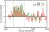 |
Fig. 1. [C II] (green) and [N II] (red) spectra extracted at the peak pixel of the line emission after continuum subtraction. The [N II] spectrum was rescaled upwards by a factor of five for easier comparison to the [C II] spectrum. The integration window used to create the line maps is shown with vertical dotted lines. |
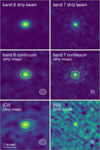 |
Fig. 2. Dirty beam (top), continuum (center), and line maps (bottom) in band 8 (left) and 7 (right) produced by the ALMA pipeline, without any cleaning applied (“dirty” images). Line maps are continuum-subtracted and were produced by summing the flux in a 800 km s−1 velocity window centered on the [C II] mean velocity. The half-intensity area of the corresponding dirty beams are shown in the bottom-right corner of each panel. Contours shown are 3σ (dotted line) and 10σ (solid line). |
3. Spatial profile modeling
3.1. Description of the modeling
Using custom-build software, we then modeled each line map independently in the image domain. We did not attempt to model the maps directly in the visibility domain for two reasons; first, fitting complex profiles other than Gaussians and point sources in the visibility domain is particularly challenging and time-consuming, and second, it has been shown that image-based and visibility-based methods actually provide similar results for ALMA data (Hodge et al. 2016). Nevertheless, we double check in Sect. 3.2 the result of our modeling against the observed visibilities.
Our model consists of a large grid of two-component exponential profiles. The first “central” component was given a small scale-length of 0.1 to 0.5 kpc to represent an unresolved central region (S18 showed the continuum emission extends over a ∼0.7 kpc half-light radius), while the scale length of the second “extended” component was permitted to vary between 0.15 and 3 kpc, with the constraint that its scale length must be at least 0.05 kpc larger than that of the central component1. We let the flux of each component vary independently and freely, with the sole constraint that the combined light profile must remain positive at all positions. We also varied the axis ratio and the position angle, however, to save on computation time, we forced the values of both components to match. Finally, the position of both components was fixed to the centroid of the continuum emission. Since the size of the galaxy is small compared to the image pixel size, we generated models with a ×9 oversampling factor and a further ×3 oversampling for the central 3 × 3 pixels to properly sample the exponential core. This corresponds to an oversampled pixel size of 0.01 (band 6) and 0.02 kpc (band 8) at the core. We then convolved the model with the ALMA dirty beam, and selected the best-fit model using maximum likelihood estimation, accounting for spatially-correlated noise in the computation of the likelihood (see Appendix C).
To estimate the uncertainty on the model, we used Monte Carlo simulations: the whole procedure was repeated 200 times on mock images that were created by perturbing the observed images with realistic noise (same amplitude and same covariance as in the real data, see Appendix A), leading to 200 other “acceptable” models from which we estimated confidence intervals using the 16th and 84th percentiles (see Appendix E). Because the distributions of the observables derived from this modeling (e.g., the ionized gas fraction) can be strongly non-Gaussian, we carried out all our calculations on each of the 200 Monte Carlo realizations and we derived confidence intervals for all derived quantities in the same fashion throughout the paper. With 200 Monte Carlo simulations, the 1σ asymmetric error bars have an accuracy of 10%.
3.2. Validation of the image-domain modeling
Since we performed all our analysis in the image-domain, we checked that the same trends we detect in this analysis are present in the raw ALMA visibilities. To do so, we used CASA to perform continuum subtraction in the visibility domain using uvcontsub (first order polynomial), excluding channels containing the line in the fit. From the resulting measurement set, we then extracted and averaged the frequency channels covered by the line using split. We note that this data set is not strictly equivalent to the image-domain data we used in our analysis, where the continuum subtraction and frequency averaging were performed in the image domain – with slightly different weights computed from the image root mean square (rms) in each channel. The images created from these alternative measurement sets have 10−20% larger noise RSM; the S/N will, therefore, be lower here than in our main analysis, but this is nevertheless sufficient for our purpose.
Ultimately, we extracted the visibilities using ms.get data() and manually performed the remaining averaging (polarization) and the binning by (u, v) distance. The real and imaginary parts of the given visibilities were averaged separately in each bin, using the weights in the measurement set, and combined to make up the binned amplitude. The uncertainties on the binned amplitudes were estimated from the weighted standard deviation of the data in the bin and scaled down by the square root of the number of points.
In parallel, we also produced mock visibilities for our best-fit and Monte Carlo models and binned them in a similar way. The corresponding visibilities were obtained from the (×9) oversampled model images created by our fitting procedure. These visibilities were computed and injected into the real measurement set using the CASA task ft, which generates mock measurement sets with the exact same (u, v) coverage and weights as the real data. To correct for any discrepancies in the data reduction between these visibilities and the images that we derived the models from, we applied a global rescaling factor to our best-fit model amplitudes to optimally match the observed visibilities.
The binned amplitudes are shown in Fig. 3. These figures demonstrate that the [C II] emission is clearly resolved. The [N II] emission is more noisy, but appears more compact and consistent with being unresolved. The best-fit models obtained from the image-domain analysis provide good matches to the visibility data, but seem mutually inconsistent between the two lines. In fact, in trying to fit the [C II] data with the [N II] model, we obtained a worse χ2 (22.4, vs 20.9 for the best-fit [C II] model), and similarly for the [N II] data and the [C II] model (15.0, vs 8.0 for the best fit [N II] model). This implies that the two emission lines have different spatial distributions, a point we analyze in greater detail in Sect. 4.
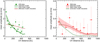 |
Fig. 3. Binned amplitude of the ALMA visibilities as a function of the UV distance (u2 + v2). The [C II] visibilities are shown on the left (green) and the [N II] visibilities are shown on the right (red). Observed visibilities are displayed as filled circles with error bars; for clarity, the visibilities on long baselines, which have large uncertainties, are not displayed. The best-fit models obtained in this paper (from the image-domain analysis) are shown as solid lines (green for [C II], red for [N II]). For comparison purposes, on each panel, the model of the other line is also displayed, but re-normalized to fit the observed visibilities. The 1σ confidence interval of the model (determined from our Monte Carlo simulations) is shown as a shaded region in the background. |
3.3. Aperture fluxes
We first applied our model to the new continuum image from band 7, which has a higher S/N and sharper angular resolution than the band 8 data used in S18. Using this modeling, we updated the dust continuum half-light radius to 0.51 ± 0.07 kpc (major axis), which is consistent with the value obtained from the band 8 data. This value was used to separate the emission into two components: “center” and “outskirts”, decribed below.
Returning to the other images (line and continuum maps), we summed the flux of every model (both for the best fit and the 200 Monte Carlo simulations) in two circular annuli: from 0 to 0.5 kpc for the “central” annulus and from 0.5 to 3.5 kpc for the “outskirts” annulus. We note that the central annulus actually contains more than half (∼75%) of the continuum emission since the model axis ratio is lower than one.
The obtained “central” and “outskirts” fluxes (for both lines and continua) are the main measurements we use in the remainder of this analysis. The other parameters of the model, such as the respective size and flux of both exponential components, are effectively marginalized over and considered unimportant. Aperture fluxes are typically simpler to constrain than other shape-related model parameters because they tend to be less model-dependent. For example, the flux inside our “central” aperture depends only slightly on the adopted size for the central component; if the aperture is larger or comparable in size, it then contains all the flux from that component, no matter how that flux is distributed internally. Furthermore, the total flux in that aperture has a natural upper bound from the data. To illustrate this, we can consider the peak pixel of the image, which for [C II], contains our aperture in its entirety. Because of the convolution with the dirty beam, this pixel contains flux from both inside and outside of our aperture. Yet, even if the relative contribution of one versus the other is uncertain, neither can exceed the observed peak flux.
In this light, it may seem an overly complex process to introduce a rich two-component model in order to simply measure two aperture fluxes. We stress that this model complexity is, in fact, crucial to the assessment of the reliability of our measurement. Indeed, the constraining power of our data (owing both to S/N and angular resolution) is not sufficient to allow us to determine the exact shape of the intensity profile at all radii. Therefore, by exploring as wide a range of models as possible – including numerous models that are barely distinguishable among the ALMA images – we make sure our uncertainties on the aperture fluxes encompass all credible scenarios permitted by the data.
To test our method and the accuracy of our uncertainties, we applied our full measurement procedure to simulated images with injected sources, as described in Appendix D. We found that our method can recover the total, central, and outskirts fluxes in all our simulated images with no detectable systematic bias. The estimated uncertainties from Monte Carlo simulations were found to correctly capture the noise in our measurements, with, at most, a 10% underestimation.
4. Results
4.1. Spatial distribution of the lines
In Fig. 4 (left panel), we show the surface brightness profile of Hyde inferred from our two-component model for the dust continuum and the two emission lines, [C II] and [N II]. Although the S/N of the [N II] data is low, when combined with the sharper angular resolution of the band 7 data it is nonetheless sufficient to demonstrate that most of the emission is centrally-concentrated, with a profile that is similar to that of the dust continuum. The [C II] emission, however, appears more extended (as is commonly found in the literature; see, e.g., Gullberg et al. 2018; Rybak et al. 2019; Tadaki et al. 2019). The intrinsic half-light radii we obtained for the continuum, [C II], and [N II] are (respectively) r1/2 = 0.51 ± 0.07, 1.2 ± 0.3, and  kpc (along the major axis). The lower error bar on the [N II] size is limited by the minimum source size in our model grid, 0.1 kpc; the data are consistent with the [N II] emission being point-like.
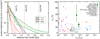 |
Fig. 4. Left: modeled intrinsic surface brightness profiles of Hyde in the dust continuum (black, horizontal stripes), [C II] (green, +45° stripes), and [N II] (red, −45° stripes). The dust continuum half-light radius is indicated with a vertical dotted black line. The PSF HWHM of the [C II] (resp. [N II]) line map is indicated with vertical dot dashed (resp. dashed) green (resp. red) line. The hashed regions show the 1σ confidence intervals obtained from the 200 mock noise realizations and are centered on the best-fit model. Right: ionized gas fraction (f[C II],ion) determined from the [C II]/[N II] line ratio in different regions of Hyde (green circles; center, outskirts, and total), compared to other values reported in the literature. For all galaxies, the ionized gas fraction was computed assuming a fixed [C II]ion/[N II]ion = 2.80 ± 0.18 (see text). We show literature values for local ETGs (red circles) and KINGFISH galaxies (purple circles) from Lapham et al. (2017), local infrared luminous galaxies in GOALS (black circles) from Zhao et al. (2016) and Díaz-Santos et al. (2017), and HERCULES from Rosenberg et al. (2015) and Kamenetzky et al. (2016), and high-redshift SMGs from Pavesi et al. (2016). We also show the upper limit of Zhang et al. (2018), obtained by stacking high-redshift lensed SMGs (downward-pointing orange triangle). |
Martí-Vidal et al. (2012) quantify what we should be able to measure in our data given the angular resolution and S/N: based on their Eq. (7), our data should be able to distinguish, with more than 95% reliability (2σ), between a point source and an extended profile with a size of 0.30, 0.96, and 0.94 kpc, respectively. The sizes of the continuum and [C II] are both larger than these values and are indeed “measured” (r/σr = 7 and 4, respectively), and the size we report for [N II] indeed has a 2σ upper limit of 0.9 kpc. Our measurements are thus consistent with these theoretical expectations.
To further confirm this difference in half-light radii with a simpler, independent method, we used the simulated noise maps described in the previous section and injected mock sources of sizes matching the values above and convolved with the dirty beam. For each mock source, we computed its observed radial profile on the noisy image and located the radius at which the emission falls below half of the peak. Comparing this simulation to the values observed on the real images, we found that the [C II] emission is significantly (3.6σ) larger than the continuum, and that [N II] is significantly (2.4σ) smaller than [C II], while the difference between [N II] and the continuum is only marginal (1.2σ).
This confirms that the difference in size between the [C II] and [N II] emission is not simply due to noise and implies the presence of a strong gradient in the [C II]/[N II] ratio, with inner regions having lower values of [C II]/[N II] and, therefore a higher proportion of ionized gas.
To quantify the gradient in the line ratio, we now turn to the measured fluxes. We list the measured values and their uncertainties in Table 1 and provide, in Appendix E, the full observed distributions in the Monte Carlo simulations, which we use to determine and propagate uncertainties throughout this paper. We found no significant flux in [N II] beyond our fiducial 0.5 kpc radius, and conversely, we found less than half of the [C II] flux is located inside this radius. This leads to a line ratio in the central region of ![$ {[\text{C}\,\small{\rm II}]}_{\mathrm{center}}/{[\text{N}\,\small{\rm II}]}_{\mathrm{center}} = 4.8^{+2.4}_{-1.7} $](/articles/aa/full_html/2021/02/aa36460-19/aa36460-19-eq3.gif) and a lower limit on the line ratio in the outskirts of [C II]outskirts/[N II]outskirts > 15 (1σ limit).
and a lower limit on the line ratio in the outskirts of [C II]outskirts/[N II]outskirts > 15 (1σ limit).
Measured line fluxes from the image analysis, corresponding ionized gas fractions, and infrared luminosities.
4.2. Ionized gas distribution
Using the fluxes estimated in the previous section, we estimated the fraction of [C II] emission associated with ionized gas (or “ionized gas fraction” for short), f[C II],ion, following a method similar to that of Díaz-Santos et al. (2017) and Lapham et al. (2017):
![$$ \begin{aligned} f_{[\mathrm{C}\,\small{\rm II}],\mathrm{ion}}= \frac{[\mathrm{C}\,\small{\rm II} ]_{\mathrm{ion} }/[\mathrm{N}\,\small{\rm II} ]_{\mathrm{ion} }}{[\mathrm{C}\,\small{\rm II} ]/[\mathrm{N}\,\small{\rm II} ]}\cdot \end{aligned} $$](/articles/aa/full_html/2021/02/aa36460-19/aa36460-19-eq36.gif)
Here, we adopt a fixed [C II]ion/[N II]ion = 2.80 ± 0.18, which is the mean value found by Lapham et al. (2017). In principle, this ratio has a weak dependence on the electron density, which can be measured using the [N II]122/[N II]205 ratio, but the [N II]122 line is not observable for Hyde due to poor atmospheric transmission at that redshifted wavelength. If Hyde turns out to have an unusual electron density, based on the modeling of Lapham et al. (2017), its [C II]ion/[N II]ion could only be higher, up to [C II]ion/[N II]ion = 4, which would only increase the value of f[C II],ion we infer from the data.
In Fig. 4 (right), we display the ionized gas fraction of Hyde in the “central” and “outskirts” annuli (which, we recall, correspond to inside and outside of the dust half-light radius, respectively). We find a clear difference between the two regions. The outskirts of the galaxy has a low f[C II],ion of 0−19%, which is typical of infrared-luminous local galaxies and distant SMGs (Pavesi et al. 2016; Díaz-Santos et al. 2017). Likewise, the L[C II]/LFIR ratio in the outskirts, ![$ \log_{10}({L_{[{\mathrm{C}\,\small{\rm II}}]}}/{L_{\text{FIR}}}) = -2.46^{+0.33}_{-0.29} $](/articles/aa/full_html/2021/02/aa36460-19/aa36460-19-eq37.gif) , is similar to that observed in other distant galaxies of this luminosity (e.g., Capak et al. 2015). This suggests that the majority of the [C II] emission in the outskirts is associated with cold star-forming gas.
, is similar to that observed in other distant galaxies of this luminosity (e.g., Capak et al. 2015). This suggests that the majority of the [C II] emission in the outskirts is associated with cold star-forming gas.
On the other hand, the center of the galaxy has a high2 f[C II],ion of 38−90%, which has never been observed in a distant SMG and is rarely observed in local infrared-luminous galaxies. Finding such high f[C II],ion is instead not uncommon in more normal or quiescent local galaxies, such as main-sequence galaxies and ETGs (Lapham et al. 2017). It should be noted, however, that f[C II],ion or [C II]/[N II] values from the literature are typically only quoted for galaxies as a whole and few studies prior to this one have attempted to separate the emission from the center and outskirts (see, e.g., Parkin et al. 2013 where a f[C II],ion gradient was found in M51). It is possible that higher f[C II],ion values could also be found in the center of some SMGs and other IR-luminous galaxies if they were observed with a sufficient angular resolution. This would be an interesting avenue for future observations, particularly as it could allow for the finding of Hyde-like analogs in the local Universe, which would, in turn, provide invaluable insights into the physical processes at play.
The ![$ \log_{10}({L_{[{\mathrm{C}\,\small{\rm II}}]}}/{L_{\text{FIR}}}) = -3.17^{+0.26}_{-0.28} $](/articles/aa/full_html/2021/02/aa36460-19/aa36460-19-eq38.gif) in the center of Hyde is also a factor of five lower than in the outskirts, which is expected if the gas is predominantly ionized (Díaz-Santos et al. 2017). This supports the hypothesis that the majority of the [C II] emitting gas in the galaxy center is ionized and not star-forming, and, therefore, that an energy source other than ongoing star formation is significantly contributing to the energy budget in the center of the galaxy. If Hyde is indeed on the path to quenching, this would strongly suggest an inside-out quenching channel.
in the center of Hyde is also a factor of five lower than in the outskirts, which is expected if the gas is predominantly ionized (Díaz-Santos et al. 2017). This supports the hypothesis that the majority of the [C II] emitting gas in the galaxy center is ionized and not star-forming, and, therefore, that an energy source other than ongoing star formation is significantly contributing to the energy budget in the center of the galaxy. If Hyde is indeed on the path to quenching, this would strongly suggest an inside-out quenching channel.
We cannot determine with certainty the nature of this central ionizing source with the available data, but we can propose two likely candidates. First, the source could be a compact population of intermediate-age stars born in a recent past. Indeed, Hyde is believed to contain about 4 × 10¹⁰ M* of stars within its half-light radius (S18), and a Bruzual & Charlot (2003) single stellar population of this mass should generate an [N II]-ionizing flux with total energy ≳108 L⊙, even at advanced ages of several hundred million years, which is larger than the observed central [N II] luminosity,  . However, hydrogen and carbon are also expected to consume part of this ionizing flux. Determining whether this is indeed a viable hypothesis would require dedicated modeling, a measure of the gas metallicity, and a better understanding of the geometry of the system, which are all lacking at present.
Second, the ionizing source could be an active galactic nucleus (AGN). Since none of the available data indicate the presence of an AGN in this galaxy (LX < 1044 erg s−1; Civano et al. 2016, L1.4 GHz < 1024 W Hz−1; Smolčić et al. 2017), this may seem less likely, yet a weak or obscured AGN cannot be ruled out. The presence of an AGN would make the interpretation of the observed line ratios more difficult and could invalidate some of the assumptions and finer calculations presented in the following section, which only account for stellar ionization flux. Yet, the implication on the galaxy’s SFR estimate would follow a similar path: if an AGN exists in the center of this galaxy, with a luminosity large enough to affect the continuum and line emission, it would necessarily contribute to the observed LIR. This, in turn, would imply that SFR estimates using LIR would be biased high. This would include our initial estimate from S18, which already tentatively placed the galaxy below the galaxy main sequence. If an AGN is indeed present, and given the large amount of dust and the compactness of the galaxy, the AGN radiation could be trapped (e.g., Costa et al. 2018) and could be coupled efficiently with the gas to suppress star formation.
4.3. Revised star formation rate
We now use the characterization of the ionizing emission presented in the previous section to provide a refined estimate of the galaxy’s SFR. We do so by estimating the infrared luminosity produced in birth clouds by young stars and feed this luminosity into our SED modeling as a prior.
The total infrared luminosity, LIR, is a very useful observable in SED modeling, as it offers an independent constraint on the obscured luminosity of a galaxy. This is particularly crucial for constraining the SFR. However, like [C II], the LIR can originate from different regions in the galaxy. Here, we consider two main contributors: birthclouds (BC), which are heated exclusively by stars younger than 10 Myr (Charlot & Fall 2000) and the inter-stellar medium (ISM), which is heated by the older stars (e.g., da Cunha et al. 2008). We label the corresponding infrared luminosities LIR, BC and LIR, ISM, respectively. LIR, BC is the quantity we aim to estimate, as by definition it most directly traces the recent SFR.
Next, we need to estimate the fraction of the infrared luminosity produced in the ISM, fIR, ISM = LIR, ISM/LIR. Intuitively, we can expect this fraction to be closely related to f[C II],ion, which we computed earlier, since PDRs are co-located with birthclouds, and since ionized gas is part of the ISM. Thus, in what follows, we assume L[C II],ion = L[C II],ISM and L[C II],PDR = L[C II],BC.
With these assumptions, we can relate fIR, ISM = LIR, ISM/LIR to f[C II],ion, using the following relation:
![$$ \begin{aligned} \frac{1}{f_{\rm IR,ISM}} - 1 = \frac{L_{\rm IR,BC}}{L_{\rm IR,ISM}}&= \frac{L_{\rm IR,BC}}{L_{[\mathrm{C}\,\small{\rm II} ],\mathrm {BC}}}\,\frac{L_{[\mathrm{C}\,\small{\rm II} ],\mathrm {ISM}}}{L_{\rm IR,ISM}}\,\frac{L_{[\mathrm{C}\,\small{\rm II} ],\mathrm {BC}}}{L_{[\mathrm{C}\,\small{\rm II} ],\mathrm {ISM}}} \nonumber \\&=\frac{([\mathrm{C}\,\small{\rm II} ]/\mathrm{IR})_{\rm ISM}}{([\mathrm{C}\,\small{\rm II} ]/\mathrm{IR})_{\rm BC}}\,\left(\frac{1}{f_{\rm [\mathrm{C}\,\small{\rm II}\mathrm ],ion}} - 1\right) \nonumber \\&= \alpha \,\left(\frac{1}{f_{\rm [\mathrm{C}\,\small{\rm II}\mathrm ],ion}} - 1\right)\cdot \end{aligned} $$](/articles/aa/full_html/2021/02/aa36460-19/aa36460-19-eq40.gif)
We can determine α empirically using a set of reference galaxies for which we can estimate both f[C II],ion and fIR,ISM. Here we used the local infrared-luminous galaxies from GOALS (Díaz-Santos et al. 2017), which have direct measurements of [C II] and [N II] from Herschel and an average of f[C II],ion = 12.6 ± 0.7%, similar to high-z SMGs. Based on the short gas depletion times typically observed for starbursting galaxies (e.g., Béthermin et al. 2015), we assumed that the GOALS galaxies were mostly formed in a brief burst lasting 50 to 200 Myr3. We then used the Bruzual & Charlot (2003) stellar populations and the uniform Calzetti et al. (2000) dust screen to compute the expected fraction of their bolometric luminosity produced by young stars for such star-formation histories, fbol, BC = 65 ± 5%. Young stars are defined as stars younger than 10 Myr, as given above. Based on the strong attenuation in these galaxies (Howell et al. 2010), the bolometric luminosity is practically equal to the infrared luminosity, and this latter fraction can thus be identified as 1 − fIR,ISM for GOALS galaxies. Feeding these estimates back to Eq. (2) gives log10(α) = − 0.57 ± 0.10 (in other words, the [C II]/IR ratio is a factor of four times lower in the ambient ISM than in birthclouds).
With the knowledge of fIR,ISM, which we can compute independently in the center (fIR,ISM = 69−96%) and outskirts (fIR,ISM = 0−46%) of Hyde, we can estimate the summed infrared luminosity produced in birth clouds for both regions: log10(LIR, BC/L⊙)=11.52 ± 0.20. We then ran FAST++4 v1.3 to model the multi-wavelength photometry with the same setup as in S18, but using LIR, BC as a prior on the obscured luminosity of stars younger than 10 Myr. Briefly, in S18, we used a flexible model for the star-formation history, formulated as an exponentially rising SFR followed by an exponential decline, with a variable time of transition between the two phases and variable exponential timescales.
The outcome is illustrated in Figs. 5 and 6. The stellar mass was essentially unaffected, but the updated model produced an  yr−1 (averaged over the last 10 Myr), which is non-zero. This leads to
  Gyr−1. With a main-sequence locus at sSFR = 2.8 Gyr−1 (Schreiber et al. 2017), this places the galaxy a factor of 4.0 below the main sequence, with a lower limit of > 2.3 at 68% confidence (and just > 1.3 at 90% confidence).
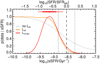 |
Fig. 5. Likelihood of the photometric data for Hyde as a function of sSFR = SFR/M*. The likelihood is shown without any constrain on the dust luminosity (gray), using the total infrared luminosity LIR (orange), or using the birthcloud infrared luminosity LIR, BC (red). The horizontal red lines show the 68% (thick) and 90% (thin) confidence intervals. The vertical lines indicate the locus of the galaxy main-sequence and its scatter from Schreiber et al. (2017). |
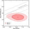 |
Fig. 6. Updated location of Hyde with respect to the galaxy main-sequence. The dashed (resp., dotted) line indicate the locus of the galaxy main-sequence (resp., its scatter) from Schreiber et al. (2017). The dark (resp., light) red region shows the final 68% (resp., 90%) confidence region for Hyde obtained in this paper. The red cross indicates the location of our best-fit solution. |
The previous estimate of the SFR from S18, using instead the total LIR as a constraint, only allowed us to obtain an upper limit on the SFR (see Fig. 5). The new data, however, exclude the possibility that Hyde has fully quenched (SFR ≪ SFRMS). While the 90% upper limit on the SFR is actually unchanged compared to our earlier estimates, we are finally able to constrain both sides of the SFR probability distribution and, therefore, we can give more credit to the maximum probability solution and the standard 68% confidence interval. In this light, we can claim that the SFR is now constrained to intermediate values that are a factor of 2−10 lower than the main-sequence level. Accounting for the observational uncertainty and the log-normal main-sequence scatter, the probably of observing sSFR < 0.71 Gyr−1 when randomly drawing from the main-sequence distribution is 4%.
One issue limiting the strength of this conclusion is that the location of the galaxy main sequence is not yet perfectly determined at z ∼ 4. Here, we based our comparison on the estimate from Schreiber et al. (2017) since it is also based on ALMA-derived SFRs and with stellar masses derived in a similar way; this mitigates the impact of systematic biases on both M* and SFR estimations, and makes the relative SFR difference between Hyde and the main sequence more robust. In fact, the most robust comparison would be obtained by applying the exact same method to determine the SFR for Hyde and for the main-sequence galaxies. Unfortunately, this cannot be achieved until high-quality [C II] and [N II] data are available for a representative sample of other normal galaxies. Nonetheless, even setting aside all our SFR modeling, it remains true that Hyde has a high overall [N II]/[C II] ratio compared to high-z SMGs, and that it is “special” in a number of ways (high attenuation, compact size, etc.). Based on this, we argue that most galaxies are not like Hyde and, therefore, on average, the SFR of typical main-sequence galaxies should be correct.
Nevertheless, we can quantify how much the above-cited result depends on the estimated locus and scatter of the main-sequence. If the main-sequence scatter is increased to 0.4 dex (resp. 0.5 dex), we find that the probably P of observing Hyde’s sSFR when drawing from the main-sequence distribution increases to 9% (resp. 13%). This does not appear to be supported by the observations, however, as other references in the literature typically report a lower scatter. For example, if the scatter is decreased to 0.25 dex (resp. 0.15 dex; Speagle et al. 2014; Pearson et al. 2018), P drops to 2.5% (resp. 0.5%). Similarly, if the main-sequence mean sSFR is decreased by 0.1 dex (Pearson et al. 2018), P increases to 8%. However, most references in the literature using FIR, sub-mm, or radio-based SFR estimates actually report a similar or higher mean sSFR at z ∼ 4 and log10(M*)∼10.8; with a difference of +0.1 dex (Speagle et al. 2014), +0.02 dex (Tomczak et al. 2016), +0.03 dex (Bourne et al. 2017), +0.07 dex (Leslie et al. 2020). Considering an increase of the main-sequence sSFR by 0.1 dex would decrease P to 2.3%.
5. Our result in context
5.1. A possible transition to quiescence
The modeling in the previous section allowed us to obtain a revised SFR estimate for Hyde, which confirms and refines the earlier estimate from S18. This SFR, together with the estimated large stellar mass, would place the galaxy evidently outside of the standard galaxy main-sequence and its scatter (e.g., Schreiber et al. 2017). This supports the hypothesis that the galaxy does not belong to the main sequence and that it is instead in transition to quiescence.
As in S18, we are still not able to determine the future of this galaxy with certainty; although its SFR at the time of observation does appear to be low, we cannot exclude that this only corresponds to a temporary pause in its activity. At best, we can bring forward two arguments which disfavor (but not disprove) this possibility. Firstly, the galaxy is already among the most massive individual system known at high redshift and sits beyond the knee of the stellar mass function. This implies that if its SFR does increase in the future, it cannot do so for very long. Secondly, if high-redshift galaxies commonly experience large (but temporary) fluctuations in their SFR, this would be detectable as an increase in the scatter of the galaxy-main sequence. This does not appear to be the case – at least not at z ∼ 4 (e.g., Schreiber et al. 2017).
5.2. Additional evidence
As pointed out in our introduction, Hyde compiles an unusual combination of observables as compared to other massive galaxies (or SMGs) at a similar epochs. We expand on these aspects in the following, along with a discussion of what additional observations could help confirm or contradict our results.
One particularly unusual combination is that of a lower-than-average dust temperature and a compact geometry. Hyde is indeed unusually compact; in recent sub-millimeter surveys, only 4 to 6% of SMGs turn out to have sizes as small as Hyde (e.g., Ikarashi et al. 2017; Gullberg et al. 2019). For massive star-forming galaxies in general, compact sizes are typically observed in starburst galaxies located above the galaxy main sequence (e.g., Elbaz et al. 2011). These galaxies also tend to have a higher dust temperature (e.g., Elbaz et al. 2011; Magnelli et al. 2014; Béthermin et al. 2015), which can be seen as a natural consequence of their high luminosity and compact geometry. Based on the very compact size of Hyde, we could therefore have expected to see an enhanced dust temperature, but the opposite is observed.
Indeed, when comparing to the average dust temperature of massive z ∼ 4 galaxies from Schreiber et al. (2018c), Hyde displays a temperature about 10 K lower than average. Although dust temperatures are notoriously difficult to measure (e.g., Casey 2012), in this case we can compare Hyde’s temperature to a reference which has been measured with the same method (SED fitting and SED templates) and the same wavelength coverage (from Herschel to ALMA band 7). This eliminates most of the systematics, and allows us to robustly quantity the relative difference.
In an attempt to understand these possibly conflicting observations, we can try to draw a comparison to other known galaxies. Here, we have selected the few known massive galaxies at high-redshift with a similar dust temperature of ∼30 K, and with a known spectroscopic redshift; the latter being required to measure the dust temperature accurately. The two most famous examples include GN20 (Daddi et al. 2009; Hodge et al. 2013; Tan et al. 2014) and HDF850.1 (Walter et al. 2012). These two galaxies have a half-light radius of 6−7 kpc, which is an order of magnitude larger than Hyde. This may on its own explain their lower-than-average dust temperature, although recent results suggest this could also be caused by optically-thick dust, at least for GN20 (Cortzen et al. 2020). To our knowledge, the only other reported instance of a low dust temperature combined with a compact geometry can be found in the interacting pair SGP 38326 (Oteo et al. 2016); unfortunately this system only has poor wavelength coverage, which renders the temperature uncertain (Tdust = 33−55 K). Although comparably massive, these galaxies are also an order of magnitude brighter than Hyde, hence, they would fit into the traditional picture of a starburst galaxy.
To date, therefore, the case of Hyde appears to be unique. Its low dust temperature could correspond to a softer radiation field (or, equivalently, to a low star-formation efficiency), which would match the results in this paper. However, as for GN20, it could also be caused by optically-thick dust. Disentangling the two possibilities would require an alternative measurement of the temperature (e.g., using the CO or [C I] line ratios; Cortzen et al. 2020).
6. Conclusions
In this work, we obtain new ALMA observations toward the Hyde galaxy to observe its [N II]205 emission. We show that the line emission is more concentrated in [N II] than in [C II], which implies a gradient in the ionized gas fraction. We find the center of the galaxy to be predominantly ionized, which suggests that young stars in their birth-clouds are not the dominant ionization source in the galaxy center, leaving the room for other sources, such as intermediate-age-stars or an AGN. In contrast, the outskirts are dominated by neutral gas, which suggests the [C II] emission there is mostly associated with star-forming regions. Using these new insights, we obtained an updated estimate of the galaxy’s star formation rate, placing it securely below the galaxy main sequence and, thus, possibly in transition to quiescence.
These results point toward an ongoing inside-out quenching mechanism and show that this process may start before the galaxy has fully expelled or consumed its gas reservoirs, as demonstrated by the strong obscuration of this galaxy. This confirms the importance of studying the properties of this galaxy in greater detail to better understand the process of quenching at high redshifts.
Further observations of this system would enable a better understanding of the state of the gas and of the mechanism responsible for quenching, in particular, the question of whether the galaxy hosts an AGN or not. New observations with ALMA are already scheduled, including high-resolution imaging of the dust continuum emission to establish the morphology and geometry of the galaxy, as well as [C I] for measuring the cold gas mass to study the interplay between the ionized and neutral gas reservoirs. Otherwise, the James Webb Space Telescope (JWST) could be used to look at the rest-frame optical lines, in particular Hα, to better constrain the SFR of the galaxy and obtain an estimate of the gas-phase metallicity. Unfortunately, even JWST may not have a sharp enough resolution to resolve the optical emission line profiles, which would then require larger telescopes, such as the European Extremely Large Telescope (E-ELT). Finally, deep low-frequency radio observations, for example with the LOw Frequency ARray (LOFAR), would reveal even moderate AGN activity and thus determine the role of AGNs in the high-redshift quenching process.
To go beyond the case study of this single object and determine the rate of occurrence of these features, similar observations of a sample of massive, obscured galaxies would be required. As illustrated here, finding transitioning galaxies is not an easy task, especially if most of them are strongly obscured and would not be included in the H-band selected catalogs produced from Hubble imaging. Samples of Spitzer-IRAC-selected galaxies may be more adequate (see Caputi et al. 2015; Wang et al. 2016, 2019), and in the near future, the JWST will hopefully open this search to larger samples of fainter galaxies.
As a sanity check, we also computed the f[C II],ion using the peak fluxes only; these peak fluxes are not model-dependent, but they will contain flux from both inside and outside of our central aperture; we still found a high f[C II],ion of 23−43%, see Table 1.
As shown in da Cunha et al. (2010), starbursting galaxies can also contain a component of older stars, which would also contribute to the IR emission. If true, this would increase our estimate of α from the GOALS galaxies, which would in turn decrease the final value of LIR, BC and SFR for Hyde. Our assumption is therefore conservative.
Acknowledgments
The authors want to thank the two anonymous referees for their comments that clearly improved the consistency, thoroughness, and overall quality of this paper. CS would like to thank Leah Morabito and Ian Heywood for sharing their expertise on interferometric imaging. Most of the numerical analysis conducted in this work has been performed using vif, a free and open source C++ library for fast and robust numerical astrophysics (cschreib.github.io/vif/). This paper makes use of the following ALMA data: ADS/JAO.ALMA#2015.A.00026.S and ADS/JAO.ALMA#2018.1.00216.S. ALMA is a partnership of ESO (representing its member states), NSF (USA) and NINS (Japan), together with NRC (Canada) and NSC and ASIAA (Taiwan) and KASI (Republic of Korea), in cooperation with the Republic of Chile. The Joint ALMA Observatory is operated by ESO, AUI/NRAO and NAOJ. GGK acknowledges the support of the Australian Research Council through the Discovery Project DP170103470. T.D.-S. acknowledges support from the CASSACA and CONICYT fund CASCONICYT Call 2018.
References
- Belli, S., Newman, A. B., & Ellis, R. S. 2019, ApJ, 874, 17 [CrossRef] [Google Scholar]
- Béthermin, M., Daddi, E., Magdis, G., et al. 2015, A&A, 573, A113 [NASA ADS] [CrossRef] [EDP Sciences] [Google Scholar]
- Birnboim, Y., & Dekel, A. 2003, MNRAS, 345, 349 [NASA ADS] [CrossRef] [Google Scholar]
- Bourne, N., Dunlop, J. S., Merlin, E., et al. 2017, MNRAS, 467, 1360 [NASA ADS] [Google Scholar]
- Bruzual, G., & Charlot, S. 2003, MNRAS, 344, 1000 [NASA ADS] [CrossRef] [Google Scholar]
- Calzetti, D., Armus, L., Bohlin, R. C., et al. 2000, ApJ, 533, 682 [NASA ADS] [CrossRef] [Google Scholar]
- Capak, P. L., Carilli, C., Jones, G., et al. 2015, Nature, 522, 455 [NASA ADS] [CrossRef] [Google Scholar]
- Caputi, K. I., Ilbert, O., Laigle, C., et al. 2015, ApJ, 810, 73 [NASA ADS] [CrossRef] [Google Scholar]
- Casey, C. M. 2012, MNRAS, 425, 3094 [Google Scholar]
- Chabrier, G. 2003, PASP, 115, 763 [Google Scholar]
- Charlot, S., & Fall, S. M. 2000, ApJ, 539, 718 [Google Scholar]
- Civano, F., Marchesi, S., Comastri, A., et al. 2016, ApJ, 819, 62 [Google Scholar]
- Cortzen, I., Magdis, G. E., Valentino, F., et al. 2020, A&A, 634, L14 [EDP Sciences] [Google Scholar]
- Costa, T., Rosdahl, J., Sijacki, D., & Haehnelt, M. G. 2018, MNRAS, 479, 2079 [NASA ADS] [CrossRef] [Google Scholar]
- Croton, D. J., Springel, V., White, S. D. M., et al. 2006, MNRAS, 365, 11 [NASA ADS] [CrossRef] [Google Scholar]
- da Cunha, E., Charlot, S., & Elbaz, D. 2008, MNRAS, 388, 1595 [Google Scholar]
- da Cunha, E., Charmandaris, V., Díaz-Santos, T., et al. 2010, A&A, 523, A78 [NASA ADS] [CrossRef] [EDP Sciences] [Google Scholar]
- Daddi, E., Dannerbauer, H., Stern, D., et al. 2009, ApJ, 694, 1517 [Google Scholar]
- Davé, R., Thompson, R., & Hopkins, P. F. 2016, MNRAS, 462, 3265 [NASA ADS] [CrossRef] [Google Scholar]
- Díaz-Santos, T., Armus, L., Charmandaris, V., et al. 2017, ApJ, 846, 32 [Google Scholar]
- Elbaz, D., Dickinson, M., Hwang, H. S., et al. 2011, A&A, 533, A119 [NASA ADS] [CrossRef] [EDP Sciences] [Google Scholar]
- Förster Schreiber, N. M., Genzel, R., Newman, S. F., et al. 2014, ApJ, 787, 38 [NASA ADS] [CrossRef] [Google Scholar]
- Gabor, J. M., & Davé, R. 2012, MNRAS, 427, 1816 [NASA ADS] [CrossRef] [Google Scholar]
- Genzel, R., Förster Schreiber, N. M., Rosario, D., et al. 2014, ApJ, 796, 7 [Google Scholar]
- Glazebrook, K., Schreiber, C., Labbé, I., et al. 2017, Nature, 544, 71 [NASA ADS] [CrossRef] [Google Scholar]
- Gobat, R., Strazzullo, V., Daddi, E., et al. 2012, ApJ, 759, L44 [NASA ADS] [CrossRef] [Google Scholar]
- Gullberg, B., Swinbank, A. M., Smail, I., et al. 2018, ApJ, 859, 12 [NASA ADS] [CrossRef] [Google Scholar]
- Gullberg, B., Smail, I., Swinbank, A. M., et al. 2019, MNRAS, 490, 4956 [NASA ADS] [CrossRef] [Google Scholar]
- Hodge, J. A., Carilli, C. L., Walter, F., Daddi, E., & Riechers, D. 2013, ApJ, 776, 22 [NASA ADS] [CrossRef] [Google Scholar]
- Hodge, J. A., Swinbank, A. M., Simpson, J. M., et al. 2016, ApJ, 833, 103 [Google Scholar]
- Howell, J. H., Armus, L., Mazzarella, J. M., et al. 2010, ApJ, 715, 572 [Google Scholar]
- Ikarashi, S., Caputi, K. I., Ohta, K., et al. 2017, ApJ, 849, L36 [NASA ADS] [CrossRef] [Google Scholar]
- Kamenetzky, J., Rangwala, N., Glenn, J., Maloney, P. R., & Conley, A. 2016, ApJ, 829, 93 [NASA ADS] [CrossRef] [Google Scholar]
- Kriek, M., van Dokkum, P. G., Labbé, I., et al. 2009, ApJ, 700, 221 [NASA ADS] [CrossRef] [Google Scholar]
- Labbé, I., Huang, J., Franx, M., et al. 2005, ApJ, 624, L81 [NASA ADS] [CrossRef] [Google Scholar]
- Lapham, R. C., Young, L. M., & Crocker, A. 2017, ApJ, 840, 51 [Google Scholar]
- Leslie, S. K., Schinnerer, E., Liu, D., et al. 2020, ApJ, 899, 58 [Google Scholar]
- Magnelli, B., Lutz, D., Saintonge, A., et al. 2014, A&A, 561, A86 [NASA ADS] [CrossRef] [EDP Sciences] [Google Scholar]
- Martig, M., Bournaud, F., Teyssier, R., & Dekel, A. 2009, ApJ, 707, 250 [NASA ADS] [CrossRef] [Google Scholar]
- Martí-Vidal, I., Pérez-Torres, M. A., & Lovanov, A. P. 2012, A&A, 541, A135 [NASA ADS] [CrossRef] [EDP Sciences] [Google Scholar]
- Merlin, E., Fontana, A., Castellano, M., et al. 2018, MNRAS, 473, 2098 [NASA ADS] [CrossRef] [Google Scholar]
- Oberst, T. E., Parshley, S. C., Stacey, G. J., et al. 2006, ApJ, 652, L125 [NASA ADS] [CrossRef] [MathSciNet] [Google Scholar]
- Oteo, I., Ivison, R. J., Dunne, L., et al. 2016, ApJ, 827, 34 [NASA ADS] [CrossRef] [Google Scholar]
- Parkin, T. J., Wilson, C. D., Schirm, M. R. P., et al. 2013, ApJ, 776, 65 [NASA ADS] [CrossRef] [Google Scholar]
- Pasquali, A., Ferreras, I., Panagia, N., et al. 2006, ApJ, 636, 115 [NASA ADS] [CrossRef] [Google Scholar]
- Pavesi, R., Riechers, D. A., Capak, P. L., et al. 2016, ApJ, 832, 151 [NASA ADS] [CrossRef] [Google Scholar]
- Pearson, W. J., Wang, L., Hurley, P. D., et al. 2018, A&A, 615, A146 [NASA ADS] [CrossRef] [EDP Sciences] [Google Scholar]
- Peng, Y., Maiolino, R., & Cochrane, R. 2015, Nature, 521, 192 [NASA ADS] [CrossRef] [Google Scholar]
- Rosenberg, M. J. F., van der Werf, P. P., Aalto, S., et al. 2015, ApJ, 801, 72 [NASA ADS] [CrossRef] [Google Scholar]
- Rybak, M., Calistro Rivera, G., Hodge, J. A., et al. 2019, ApJ, 876, 112 [NASA ADS] [CrossRef] [Google Scholar]
- Schreiber, C., Pannella, M., Leiton, R., et al. 2017, A&A, 599, A134 [NASA ADS] [CrossRef] [EDP Sciences] [Google Scholar]
- Schreiber, C., Glazebrook, K., Nanayakkara, T., et al. 2018a, A&A, 618, A85 [NASA ADS] [CrossRef] [EDP Sciences] [Google Scholar]
- Schreiber, C., Labbé, I., Glazebrook, K., et al. 2018b, A&A, 611, A22 [NASA ADS] [CrossRef] [EDP Sciences] [Google Scholar]
- Schreiber, C., Elbaz, D., Pannella, M., et al. 2018c, A&A, 609, A30 [NASA ADS] [CrossRef] [EDP Sciences] [Google Scholar]
- Silk, J., & Rees, M. J. 1998, A&A, 331, L1 [NASA ADS] [Google Scholar]
- Simpson, J. M., Smail, I., Wang, W., et al. 2017, ApJ, 844, L10 [NASA ADS] [CrossRef] [Google Scholar]
- Smolčić, V., Delvecchio, I., Zamorani, G., et al. 2017, A&A, 602, A2 [NASA ADS] [CrossRef] [EDP Sciences] [Google Scholar]
- Speagle, J. S., Steinhardt, C. L., Capak, P. L., & Silverman, J. D. 2014, ApJS, 214, 15 [NASA ADS] [CrossRef] [Google Scholar]
- Straatman, C. M. S., Labbé, I., Spitler, L. R., et al. 2015, ApJ, 808, L29 [NASA ADS] [CrossRef] [Google Scholar]
- Tadaki, K.-I., Iono, D., Hatsukade, B., et al. 2019, ApJ, 876, 1 [NASA ADS] [CrossRef] [Google Scholar]
- Tan, Q., Daddi, E., Magdis, G., et al. 2014, A&A, 569, A98 [NASA ADS] [CrossRef] [EDP Sciences] [Google Scholar]
- Tomczak, A. R., Quadri, R. F., Tran, K. H., et al. 2016, ApJ, 817, 118 [NASA ADS] [CrossRef] [Google Scholar]
- Walter, F., Decarli, R., Carilli, C., et al. 2012, Nature, 486, 233 [Google Scholar]
- Wang, T., Elbaz, D., Schreiber, C., et al. 2016, ApJ, 816, 84 [Google Scholar]
- Wang, T., Schreiber, C., Elbaz, D., et al. 2019, Nature, 572, 211 [Google Scholar]
- Wellons, S., Torrey, P., Ma, C., et al. 2015, MNRAS, 449, 361 [NASA ADS] [CrossRef] [Google Scholar]
- Zhang, Z., Ivison, R. J., George, R. D., et al. 2018, MNRAS, 481, 59 [NASA ADS] [CrossRef] [Google Scholar]
- Zhao, Y., Lu, N., Xu, C. K., et al. 2016, ApJ, 819, 69 [NASA ADS] [CrossRef] [Google Scholar]
Appendix A: Simulated noise maps
To estimate parameter uncertainties, the method we used in this study is based on the repetition of our measurement on mock images, created by duplicating the true image and adding different realizations of noise to it. In this experiment, the observed noisy image and our best-fit model become the “truth”, and we can determine how far away our fitting procedure is from this “truth” on each mock image. The strength of this method is that it requires no assumption on the model, and no analytical calculations; the parameter probability distribution can be extracted straight away by gathering the fits to all mock images. Furthermore, it automatically takes care of parameters that are strongly correlated with one another, as well as correlated noise. The difficulty is that it strongly depends on the quality of the noise that is injected on top of the “truth” image. For uncertainties to be accurate, the noise needs to have the exact same amplitude and covariance matrix as in the real data.
While in non-interferometric data sets the noise can usually be assumed uncorrelated, this is not the case with our ALMA data; the noise observed in the [C II] line map and its auto-correlation function (ACF), are shown in Fig. A.1 (left). We can observe that the ACF has a structure very similar to the dirty beam (see Fig. A.1, center) and we demonstrate in Appendix B that this is indeed expected when the data is imaged with natural weighting.
This makes it easy to reproduce noise with a similar covariance. Indeed, if a uniform uncorrelated random noise is convolved with a two-dimensional kernel K, its ACF will be C = K ⊗ K, or in the Fourier domain, Ĉ = K̂2 (where “hat” symbolizes the Fourier transform). If we set C = P, where P is the dirty beam (see Appendix B), we have:

Since the Fourier transform introduces aliasing artifacts on the edges of K, it is desirable to use a dirty beam image P that is significantly larger than the final dimensions of the noise map. This can be achieved by padding. To stabilize this further, and since we are mostly interested in preserving the “core” of the covariance, we smoothed out the transition to the edges of the image by multiplying the dirty beam image with a broad Gaussian of FWHM 4″.
We used this empirical convolution kernel K to generate new correlated noise realizations, shown in Fig. A.1 (right). The resulting noise maps are visually similar to the real noise map, and the core of the covariance is well reproduced. We note that since the dirty beam side lobes in our data have a relatively low amplitude, very similar results could have been achieved by simply using a Gaussian kernel of FWHM equal to half that of the dirty beam.
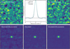 |
Fig. A.1. Observed and simulated noise maps (top) and their respective auto-correlation functions (bottom). The real [C II] map is displayed in the top left corner, with the source masked in the center. For comparison, we also display the [C II] dirty beam in the middle of the bottom panel. All the images on each row are displayed with the same color bar. The auto-correlation functions were rescaled prior to display to a peak value of unity. For easier comparison, we also show a circular average of the covariance in the central column of the first row, with the observed (black) and simulated (green dashed) auto-correlation functions, and the dirty-beam profile (blue). |
Finally, to set the noise rms, we simply measured the rms on the real image and on the simulated noise images, and rescaled the simulated images to match the real observed rms. Because our target is at the phase center, we did not correct for the primary beam attenuation in the real (or simulated) images, hence the rms was constant across the entire image.
Appendix B: Auto-correlation function of image-domain noise
For a generic interferometer, the observed dirty image is the Fourier transform of the weighted and sampled sky visibility:
![$$ \begin{aligned} I_D(x,y) \equiv &\int A(u,v)\,W(u,v)\,V(u,v)\nonumber \\&\times \exp \large [-2\pi \,i\,(u\,x + v\,y)\large ]\,\mathrm{d} u\,\mathrm{d} v, \end{aligned} $$](/articles/aa/full_html/2021/02/aa36460-19/aa36460-19-eq44.gif)
where A is the visibility sampling of the interferometer (a sum of delta functions), W is the imaging weight, and V is the complex visibility. Without loss of generality and for simplicity of notation, we drop the time, frequency, and polarization dependence in all quantities.
The dirty beam is the response to a point source, which has constant visibilities in the Fourier domain:
![$$ \begin{aligned} P(x,y)&\propto \int A(u,v)\,W(u,v)\,\exp \large [-2\pi \,i\,(u\,x + v\,y)\large ]\,\mathrm{d} u\,\mathrm{d} v. \end{aligned} $$](/articles/aa/full_html/2021/02/aa36460-19/aa36460-19-eq45.gif)
If we define the inverse Fourier transform of the dirty image:
![$$ \begin{aligned} V_D(u,v)&\equiv \int I_D(x,y)\,\exp \large [2\pi \,i\,(u\,x + v\,y)\large ]\,\mathrm{d} u\,\mathrm{d} v ,\end{aligned} $$](/articles/aa/full_html/2021/02/aa36460-19/aa36460-19-eq46.gif)

then by definition, the image auto-correlation function (ACF) is:
![$$ \begin{aligned} C(x,y)&\equiv \int V_D(u,v)\,\bar{V}_D(u,v)\,\exp \large [-2\pi \,i\,(u\,x + v\,y)\large ]\,\mathrm{d} u\,\mathrm{d} v ,\end{aligned} $$](/articles/aa/full_html/2021/02/aa36460-19/aa36460-19-eq48.gif)
![$$ \begin{aligned}&= \int A(u,v)\,W(u,v)^2\,V(u,v)\,\bar{V}(u,v)\nonumber \\&\quad \times \exp \large [-2\pi \,i\,(u\,x + v\,y)\large ]\,\mathrm{d} u\,\mathrm{d} v, \end{aligned} $$](/articles/aa/full_html/2021/02/aa36460-19/aa36460-19-eq49.gif)
where we used A2 = A since it is a sum of delta functions.
To study the ACF of the noise, we now assume that the sky contains no source and the visibilities are therefore only made of noise of amplitude σ(u, v), which we assume is uncorrelated. Thus, ⟨V V̄⟩ = σ2. If we now compute the expectation value of the ACF, we get:
![$$ \begin{aligned} \left < C(x,y)\right> =&\int A(u,v)\,W(u,v)^2\,\sigma (u,v)^2\nonumber \\&\times \exp \large [-2\pi \,i\,(u\,x + v\,y)\large ]\,\mathrm{d} u\,\mathrm{d} v. \end{aligned} $$](/articles/aa/full_html/2021/02/aa36460-19/aa36460-19-eq50.gif)
In the case of natural weighting, the weights are chosen as W ∝ 1/σ2. Injecting this into the above equation, we finally get:
![$$ \begin{aligned} \left < C(x,y)\right>&\propto \int A(u,v)\,W(u,v)\,\exp \large [-2\pi \,i\,(u\,x + v\,y)\large ]\,\mathrm{d} u\,\mathrm{d} v ,\end{aligned} $$](/articles/aa/full_html/2021/02/aa36460-19/aa36460-19-eq51.gif)

Therefore, for images produced with natural weighting, the expectation value of the noise ACF is the dirty beam.
In practice, the match is not perfect (see Fig. A.1) and this can be explained by at least three possible causes: (a) we can only measure the ACF on a finite-sized image, so our estimate of the image ACF is noisy; (b) the σ that enters in the definition of W is only an estimate of the true visibility uncertainty; and (c) the noise in the visibilities can itself be correlated. These potential issues seem to have only a moderate impact however; as demonstrated in Fig. A.1 (middle, top), in our data the core of the ACF is extremely well reproduced by the dirty beam.
Appendix C: Likelihood for correlated Gaussian noise
The general formulation of the likelihood for Gaussian correlated noise is:
where d is a vector of observed data, m is a vector of model data, and Σ is the data covariance matrix (symmetric and positive definite). For our data (see Appendix B), we have:
where σ is the image rms, (xi, yi) are the image coordinates of pixel i, and P(δx, δy) is the value of the dirty beam at an offset position (δx, δy) from the peak.
In practice, inverting Σ is numerically unstable. The best way to evaluate it is to perform a singular value decomposition (SVD), such that Σ = Uλ Ut, where U is a unitary matrix (U−1 = Ut) and λ is a diagonal matrix whose entries are the singular values λi sorted by decreasing value. Then we have Σ−1 = Uλ−1 Ut. If we define  , then Eq. (C.1) can be rewritten in a simpler form:
where  and
and  . These can be seen as the “de-correlated” observation and model vectors, respectively.
The SVD is not sufficient to make the computation of Σ−1 or L−1 stable. In all cases, the matrix λ contains small entries that cannot be inverted safely. A workaround is to truncate the matrix  by setting to zero the inverse of those singular values that are smaller than some chosen threshold. The resulting matrix inverse is then a “pseudo-inverse” (i.e., an approximation of the true inverse), but it is usually better behaved.
The method we adopted to choose the threshold is the following. We defined the normalized singular values  , and we created a logarithmic grid of 100 threshold values v ranging from
  to 0.1, such that all
  were removed from the inverse. For each value of v, we evaluated the corresponding L−1, and used it to “de-correlate” one of our noise realization from the simulations (this noisy image did not contain any source). We computed the covariance matrix of the resulting image, normalized it to unit diagonal, and defined the metric k as the sum the absolute value of entries with |xi − xj|≤1 and |yi − yj|≤1. We then picked the value of v which minimized k, or in other words, the value which produced an image with the lowest noise covariance. Experiments showed that k is large when v is too small, as the matrix inverse is unstable and the resulting images are degraded. On the other hand, k is also large when v is too large, as this leads to a poorer approximation of the inverse which leaves more correlated noise.
We note that while Eq. (C.1) is formally the correct expression to compute the likelihood for our data, we obtained very similar results when we used the simpler, standard expression for uncorrelated noise, χ2 = ∑i [(di − mi)/σ]2. This is because we used Monte Carlo simulations to determine the confidence intervals rather than relying on the shape of the likelihood.
Appendix D: Input/output simulations
To test the accuracy of our profile-fitting method, we performed an input/output analysis, where we placed sources of known light profiles in simulated noise maps devoid of sources, and tried to recover their profile with our method. The input sources were modeled as two-component exponential disks, with a small “core” component and an “extended” component, as is assumed in our model. The size of the “core” component was chosen randomly in the range, rcore = 0.1−0.5 kpc, and the size of the extended component was chosen randomly in the range, rextended = rcore + 0.2−2.2 kpc. The relative flux of these components was chosen uniformly between 0% (all flux in extended component) to 100% (all flux in core component). The axis ratio was chosen randomly between 0.4 and 1.0, and the position angle could take any value. Finally, the peak flux of each source was matched to the observed peak flux in our real images. As for our real data, we then computed the true fluxes inside and outside of a 0.5 kpc aperture to obtain the “central” and “outskirts” fluxes. We note here that since the [N II] image has a sharp angular resolution, the step of fixing the peak flux in the simulations has a strong impact on the true flux in the central aperture, as can be seen in Fig. D.1 where the range of Fcenter is limited. This is less true for [C II], where the coarser PSF means that the central pixel can contain more flux from the extended component.
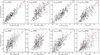 |
Fig. D.1. Outcome of the input/output analysis of our fitting procedure, modeling sources of known profiles in mock images. The simulations matching the [C II] and [N II] maps are shown at the top and bottom, respectively. From left to right: we show how our method recovers the total flux, the flux inside the center, the flux in the outskirts, and the ratio of center-to-total (with “center” and “outskirts” as defined in the main text). The red line is the line of perfect agreement. |
The mock sources were injected directly in the image domain, by convolving the source’s known light profile with the image dirty beam at ×9 oversampling. To test the accuracy of this source injection method, we also used CASA to create simulated visibilities for each mock source using simobserve (without thermal noise) and produced corresponding dirty images using clean with the same (oversampled) cell size. The resulting mock images looked identical to those produced by convolution with the dirty beam. To quantify this property, for each mock source we computed the second moment (R2) of the images produced by the two methods (visibilities imaging, and image convolution). We found a maximum relative error on R2 of only 3 × 10⁻⁵, that is, close to numerical noise, with no dependence on the size of the mock sources. This implies that injecting directly in the image domain is an accurate source injection method, which is also much faster than creating mock visibilities and imaging them. We caution that this property only holds because we work with dirty images; such images can be described as a Fourier transform of an incomplete (u, v) plane, but cleaned images cannot.
We repeated this procedure with 200 different mock sources, and for each source we replicated the noise level, noise covariance matrix, peak flux, and dirty beam of the [C II], [N II], and continuum maps separately, to test the impact of the varying S/N and angular resolutions encountered in this work. Our fitting procedure was then applied to each of these mock sources and the recovered profiles were compared to the real ones. Since these simulations are accurate mocks of the real images, they allow us to reproduce exactly the measurements we perform in this paper, so we can study any bias arising from our method.
The outcome of this analysis, illustrated in Fig. D.1 for [C II] and [N II], shows that our modeling method recovers the total, central, and outskirts fluxes with no detectable bias. The measurements are noisy, particularly for the central flux, however the observed scatter is correctly captured by the error bars, which were estimated exactly the same way as for the real data. To quantify this, for each observed quantity F shown in Fig. D.1, we computed the normalized residual δF = (Fobs − Ftrue)/σobs, where σobs is our estimated uncertainty. We then computed the fraction of simulated points with |δF|< 1. If our uncertainties are perfectly accurate, and if the noise on the quantity F is roughly Gaussian, this fraction should be equal to 68%. Since we only use 200 points to compute these fractions, the expected statistical error on this number is about 3%. We find fractions for [C II] (resp. [N II]) of 67% (resp. 66%) for the total flux, 62% (resp. 61%) for the flux in the inner 0.5 kpc, and 61% (resp. 62%) for the flux in the outskirts. These values are exactly in the expected range for the total flux, but the fractions for the central and outskirts fluxes are slightly lower than 68%. For Gaussian noise, this would imply that the uncertainties are under-estimated by at most 10%; taking this small correction into account would not affect our conclusions.
Appendix E: Parameter distributions in the Monte Carlo simulations
 |
Fig. E.1. Joint distribution of the fluxes, flux ratios, and ionized gas fraction in the Monte Carlo simulations executed for the real images. As is customary, on the diagonal we show the histogram of each quantity; the y-axis for these plots is scaled automatically to include the maximum counts in a bin. The green horizontal bars correspond the 16th and 84th percentiles, which we report as uncertainties, and the horizontal green bar is the best-fit value. |
All Tables
Measured line fluxes from the image analysis, corresponding ionized gas fractions, and infrared luminosities.
All Figures
|
Fig. 1. [C II] (green) and [N II] (red) spectra extracted at the peak pixel of the line emission after continuum subtraction. The [N II] spectrum was rescaled upwards by a factor of five for easier comparison to the [C II] spectrum. The integration window used to create the line maps is shown with vertical dotted lines. |
| In the text | |
|
Fig. 2. Dirty beam (top), continuum (center), and line maps (bottom) in band 8 (left) and 7 (right) produced by the ALMA pipeline, without any cleaning applied (“dirty” images). Line maps are continuum-subtracted and were produced by summing the flux in a 800 km s−1 velocity window centered on the [C II] mean velocity. The half-intensity area of the corresponding dirty beams are shown in the bottom-right corner of each panel. Contours shown are 3σ (dotted line) and 10σ (solid line). |
| In the text | |
|
Fig. 3. Binned amplitude of the ALMA visibilities as a function of the UV distance (u2 + v2). The [C II] visibilities are shown on the left (green) and the [N II] visibilities are shown on the right (red). Observed visibilities are displayed as filled circles with error bars; for clarity, the visibilities on long baselines, which have large uncertainties, are not displayed. The best-fit models obtained in this paper (from the image-domain analysis) are shown as solid lines (green for [C II], red for [N II]). For comparison purposes, on each panel, the model of the other line is also displayed, but re-normalized to fit the observed visibilities. The 1σ confidence interval of the model (determined from our Monte Carlo simulations) is shown as a shaded region in the background. |
| In the text | |
|
Fig. 4. Left: modeled intrinsic surface brightness profiles of Hyde in the dust continuum (black, horizontal stripes), [C II] (green, +45° stripes), and [N II] (red, −45° stripes). The dust continuum half-light radius is indicated with a vertical dotted black line. The PSF HWHM of the [C II] (resp. [N II]) line map is indicated with vertical dot dashed (resp. dashed) green (resp. red) line. The hashed regions show the 1σ confidence intervals obtained from the 200 mock noise realizations and are centered on the best-fit model. Right: ionized gas fraction (f[C II],ion) determined from the [C II]/[N II] line ratio in different regions of Hyde (green circles; center, outskirts, and total), compared to other values reported in the literature. For all galaxies, the ionized gas fraction was computed assuming a fixed [C II]ion/[N II]ion = 2.80 ± 0.18 (see text). We show literature values for local ETGs (red circles) and KINGFISH galaxies (purple circles) from Lapham et al. (2017), local infrared luminous galaxies in GOALS (black circles) from Zhao et al. (2016) and Díaz-Santos et al. (2017), and HERCULES from Rosenberg et al. (2015) and Kamenetzky et al. (2016), and high-redshift SMGs from Pavesi et al. (2016). We also show the upper limit of Zhang et al. (2018), obtained by stacking high-redshift lensed SMGs (downward-pointing orange triangle). |
| In the text | |
|
Fig. 5. Likelihood of the photometric data for Hyde as a function of sSFR = SFR/M*. The likelihood is shown without any constrain on the dust luminosity (gray), using the total infrared luminosity LIR (orange), or using the birthcloud infrared luminosity LIR, BC (red). The horizontal red lines show the 68% (thick) and 90% (thin) confidence intervals. The vertical lines indicate the locus of the galaxy main-sequence and its scatter from Schreiber et al. (2017). |
| In the text | |
|
Fig. 6. Updated location of Hyde with respect to the galaxy main-sequence. The dashed (resp., dotted) line indicate the locus of the galaxy main-sequence (resp., its scatter) from Schreiber et al. (2017). The dark (resp., light) red region shows the final 68% (resp., 90%) confidence region for Hyde obtained in this paper. The red cross indicates the location of our best-fit solution. |
| In the text | |
|
Fig. A.1. Observed and simulated noise maps (top) and their respective auto-correlation functions (bottom). The real [C II] map is displayed in the top left corner, with the source masked in the center. For comparison, we also display the [C II] dirty beam in the middle of the bottom panel. All the images on each row are displayed with the same color bar. The auto-correlation functions were rescaled prior to display to a peak value of unity. For easier comparison, we also show a circular average of the covariance in the central column of the first row, with the observed (black) and simulated (green dashed) auto-correlation functions, and the dirty-beam profile (blue). |
| In the text | |
|
Fig. D.1. Outcome of the input/output analysis of our fitting procedure, modeling sources of known profiles in mock images. The simulations matching the [C II] and [N II] maps are shown at the top and bottom, respectively. From left to right: we show how our method recovers the total flux, the flux inside the center, the flux in the outskirts, and the ratio of center-to-total (with “center” and “outskirts” as defined in the main text). The red line is the line of perfect agreement. |
| In the text | |
|
Fig. E.1. Joint distribution of the fluxes, flux ratios, and ionized gas fraction in the Monte Carlo simulations executed for the real images. As is customary, on the diagonal we show the histogram of each quantity; the y-axis for these plots is scaled automatically to include the maximum counts in a bin. The green horizontal bars correspond the 16th and 84th percentiles, which we report as uncertainties, and the horizontal green bar is the best-fit value. |
| In the text | |
Current usage metrics show cumulative count of Article Views (full-text article views including HTML views, PDF and ePub downloads, according to the available data) and Abstracts Views on Vision4Press platform.
Data correspond to usage on the plateform after 2015. The current usage metrics is available 48-96 hours after online publication and is updated daily on week days.
Initial download of the metrics may take a while.