| Issue |
A&A
Volume 630, October 2019
|
|
|---|---|---|
| Article Number | A110 | |
| Number of page(s) | 23 | |
| Section | Extragalactic astronomy | |
| DOI | https://doi.org/10.1051/0004-6361/201936270 | |
| Published online | 30 September 2019 | |
Radio loudness along the quasar main sequence⋆
1
Dipartimento di Fisica & Astronomia “Galileo Galilei”, Università di Padova, Padova, Italy
e-mail: valerio.ganci@gmail.com
2
National Institute for Astrophysics (INAF), Padua Astronomical Observatory, 35122 Padova, Italy
3
Instituto de Astrofisíca de Andalucía, IAA-CSIC, 18008 Granada, Spain
4
Belgrade Astronomical Observatory, 11060 Belgrade, Serbia
5
Instituto de Astronomía, UNAM DF 04510, Mexico
Received:
9
July
2019
Accepted:
19
August
2019
Context. When can an active galactic nucleus (AGN) be considered radio loud (RL)? Following the established view of the AGNs inner workings, an AGN is RL if associated with relativistic ejections emitting a radio synchrotron spectrum (i.e., it is a “jetted” AGN). In this paper we exploit the AGN main sequence that offers a powerful tool to contextualize radio properties.
Aims. If large samples of optically-selected quasars are considered, AGNs are identified as RL if their Kellermann’s radio loudness ratio RK > 10. Our aims are to characterize the optical properties of different classes based on radio loudness within the main sequence and to test whether the condition RK > 10 is sufficient for the identification of RL AGNs, since the origin of relatively strong radio emission may not be necessarily due to relativistic ejection.
Methods. A sample of 355 quasars was selected by cross-correlating the Very Large Array Faint Images of the Radio Sky at Twenty-Centimeters survey (FIRST) with the twelfth release of the Sloan Digital Sky Survey Quasar Catalog published in 2017. We classified the optical spectra according to their spectral types along the main sequence of quasars. For each spectral type, we distinguished compact and extended morphology (providing a FIRST-based atlas of radio maps in the latter case), and three classes of radio loudness: detected ( specific flux ratio in the g band and at 1.4 GHz, R′K < 10), intermediate (10 ≤ R′K < 70), and RL (R′K ≥ 70).
Results. The analysis revealed systematic differences between radio-detected (i.e., radio-quiet), radio-intermediate, and RL classes in each spectral type along the main sequence. We show that spectral bins that contain the extreme Population A sources have radio power compatible with emission by mechanisms ultimately due to star formation processes. RL sources of Population B are characteristically jetted. Their broad Hβ profiles can be interpreted as due to a binary broad-line region. We suggest that RL Population B sources should be preferential targets for the search of black hole binaries, and present a sample of binary black hole AGN candidates.
Conclusions. The validity of the Kellermann’s criterion may be dependent on the source location along the quasar main sequence. The consideration of the main sequence trends allowed us to distinguish between sources whose radio emission mechanisms is jetted from the ones where the mechanism is likely to be fundamentally different.
Key words: Galaxy: evolution / quasars: general / quasars: emission lines / quasars: supermassive black holes / accretion / accretion disks / galaxies: jets
Tables A.1–A.3 are only available at the CDS via anonymous ftp to cdsarc.u-strasbg.fr (130.79.128.5) or via http://cdsarc.u-strasbg.fr/viz-bin/cat/J/A+A/630/A110
© ESO 2019
1. Introduction
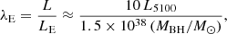
The main sequence (MS) of quasars has proved to be a powerful tool to contextualize the observational properties of type-1 active galactic nuclei (AGNs; see Sulentic & Marziani 2015 for a recent review). The MS concept stemmed from an application of the Principal Component Analysis to quasar spectra (Boroson & Green 1992) that yielded a first fundamental correlation vector (called the Eigenvector-1, E1) of type-1 AGNs. More precisely, the E1 is associated with anti-correlations between the strength of FeIIλ4570 and the [O III]λ5007 peak intensity, and between strength of FeIIλ4570 and the full width at half maximum (FWHM) of Hβ (Boroson & Green 1992). The FeIIλ4570 strength is usually represented by the parameter RFeII= I(FeIIλ4570)/I(Hβ), the ratio between the integrated flux of the FeIIλ4570 blend of multiplets between 4434 Å and 4684 Å, and that of the Hβ full broad component. The full broad component refers to the full profile without the narrow component, that is, as in previous works (e.g., Brotherton et al. 1994; Corbin & Boroson 1996; Bon et al. 2006; Hu et al. 2008; Li et al. 2015; Adhikari et al. 2016), subdivided into a broad (HβBC) and a very-broad component (HβVBC). The distribution of data points in the E1 optical plane, or in other words FWHM(Hβ) vs. RFeII, defines the quasar MS, in analogy to the stellar MS on the Hertzsprung–Russell diagram (Sulentic et al. 2001a,b, 2008; Shen & Ho 2014).
The shape of the MS for quasars of luminosity L ≲ 1047 erg s−1, and z < 0.7 allows for the subdivision of the optical E1 plane into two populations, and a grid of bins of FWHM(Hβ) and RFeII, that defines a sequence of spectral types (STs; see the sketch in Fig. 1). Population A (FWHM(Hβ) ≤ 4000 km s−1) and B (FWHM(Hβ) > 4000 km s−1) separate different behaviors along the E1 sequence, possibly associated with differences in accretion modes (e.g., Wang et al. 2014; Du et al. 2016a, and references therein). Population A STs are defined in terms of increasing RFeII with bin size ΔRFeII = 0.5. Spectral types from A1, with RFeII ≤ 0.5, to A4, with 1.5 < RFeII ≤ 2.0 account for almost all Population A sources, save for a few FeII-strong “outliers” (Lipari et al. 1993; Graham et al. 1996; Marziani et al. 2013). Population B STs are defined in terms of increasing FWHM Hβ with ΔFWHM(Hβ) = 4000 km s−1. Spectral types from B1 (4000 < FWHM(Hβ) ≤ 8000 km s−1), to B1++ (12 000 < FWHM(Hβ) ≤ 16 000 km s−1) account for the wide majority of Population B sources. Spectral types are intended to isolate sources with similar broad-line physics and/or viewing angle. From here onwards, we will consider STs A3 and A4 as extreme population A (xA; the area shaded green in Fig. 1), in accordance with the recent analysis by Negrete et al. (2018).
 |
Fig. 1. Sketch illustrating definition of STs along MS, as function of RFeII and FWHM(Hβ). The numbers in square brackets yield from top to bottom, the prevalences of each spectral bin (nST) in an optically selected sample (Marziani et al. 2013), of the RI and RL sources (nRI + RL) and of RD (nRD) in each spectral bin. The total number of sources is N = 680. The gray and pale green ares trace the source occupation in the plane; the green area separates extreme Population A from the rest of the MS. |
There is no doubt that several physical parameters affect the E1 MS. Recent works (e.g., Sulentic et al. 2011; Fraix-Burnet et al. 2017) present a list of them and of their relation to observed parameters. The physical interpretation of the MS is still being debated (Shen & Ho 2014; Panda et al. 2018), although there is a growing consensus that the main factors shaping the MS occupation in the optical plane RFeII-FWHM(Hβ) (at least for a low-z sample) are the Eddington ratio (λE) and the viewing angle defined as the angle between the line of sight and the symmetry axis of the active nucleus. RFeII correlates with metallicity, ionization conditions, density and column density, and ultimately with λE (Grupe et al. 1999; Kuraszkiewicz et al. 2009; Ai et al. 2010; Dong et al. 2011; Du et al. 2016a; Panda et al. 2019, and references therein). FWHM(Hβ) correlates with the velocity dispersion in the low-ionization lines emitting region of the broad-line region (BLR) and provides a measurement of the virial broadening associated with ionized gas motion around the central massive black hole (BH; Shen 2013, and references therein). The FWHM is affected by physical parameters such as BH mass (MBH) and λE, but also by the viewing angle (Panda et al. 2019). Growing evidence indicates that the low-ionization part of the BLR is highly flattened (Mejía-Restrepo et al. 2018, and references therein). It is therefore straightforward to think about a physically-motivated distinction between Population A and Population B. In a word, Population A sources are fast-accreting objects with a relatively small MBH (at least at low-z) and Population B are the ones with high MBH and low λE (e.g., Marconi et al. 2009; Fraix-Burnet et al. 2017).
The MS, as drawn in Fig. 1, has been built for an optically selected sample at low-z (≲1; Marziani et al. 2013), and includes both radio-quiet (RQ) and radio-loud (RL) AGNs. The behavior of the RL sources in the MS is still poorly known, since RL quasars are a minority, only ∼10% of all quasars (a fact that became known a few years after the discovery of quasars, Sandage 1965). The physical definition of RL sources involves the presence of a strong relativistic jet (i.e., sources are “jetted,” Padovani 2017), whereas in RQ sources the jet is expected to be non-relativistic or intrinsically weaker than in RL (e.g., Middelberg et al. 2004; Ulvestad et al. 2005; Gallimore et al. 2006), and other physical mechanisms due to nuclear activity could be important components. Radio-quiet sources do have a radio emission and their radio powers can be even a few orders of magnitude lower than those of their RL counterparts for the same optical power (e.g., Padovani 2016).
The presence of relativistic ejections gives rise to a host of phenomenologies over the full frequency range of the electromagnetic spectrum. Apart from the enhancement in radio power with respect to RQ quasars, differences can be seen between the hard X-ray and the γ-ray wavelength ranges. RL sources emit up to GeV (2.4 × 10²³ Hz, (Padovani 2017, Fig. 1)) energies or in some cases to TeV whereas RQ sources show a sharp cut-off at energies ∼1 MeV (e.g., Malizia et al. 2014). No RQ AGN has been detected in γ-rays (Ackermann et al. 2012). These properties let us think about two, at least in part, intrinsically different types of sources: through the accretion process, RLs emit a large fraction of their energy non-thermally over the whole electromagnetic spectrum, whereas RQ quasars emit most of their power thermally from viscous dissipation in the torus and the accretion disk.
The customary selection of RL sources is based on the ratio RK = fν, radio/fν, opt, where the numerator is the radio flux density at 5 GHz and the denominator is the optical flux density in the B band (Kellermann et al. 1989). Radio-loud sources are defined as the ones having RK > 10. The classification is made also employing a surrogate Kellermann’s parameter  with the g band and the specific radio flux at 20 cm (Sect. 2.2 and 3.1).
Applying the Kellermann’s criterion, the prevalence of RL sources is not constant along the MS. The data of Fig. 1 are from a 680-strong quasar sample (Marziani et al. 2013) from the Sloan Digital Sky Survey (SDSS) Quasar Catalog: in the 680 sample, 30% of extreme Pop. B (i.e., ST B1++) are radio intermediates (RI) or RLs; ST B1 and B1+, which include half of the sample, have a prevalence of ∼9% each consistent with previous studies (Kellermann et al. 1989; Urry & Padovani 1995; Zamfir et al. 2008). A minimum prevalence of just 2% is reached in ST A2, whereas higher RFeII ST A3 and A4 show a surprising increase. Previous works have shown that jetted sources are more frequent among Pop. B sources or, equivalently at low λE (Sikora et al. 2007; Zamfir et al. 2008). Pop. A and Pop. B sources are known to have a different spectral energy distributions (SEDs), flatter in the case of Pop. B. Zamfir et al. (2008) suggest a more restrictive criterion: RK > 70 as a sufficient condition to identify jetted sources. This criterion may indeed be sufficient but may lead to the loss of a significant number of intrinsically jetted sources. Zamfir et al. (2008) observed that “intermediate” sources with  are distributed across the whole MS. This did not explain their physical nature but did not exclude that a fraction of them could be jetted. On the other hand, ST A3 and A4 are associated with high λE and concomitant high star-formation rate (SFR; e.g., Sani et al. 2010). Star forming processes are believed to be associated with accretion in RQ quasars (e.g., Sanders et al. 2009). They become most evident in the far-infrared (FIR) domain of their SED (e.g., Sanders et al. 1988; Haas et al. 2003; Sani et al. 2010). High SFR leads to correspondingly high radio power (e.g., Condon 1992; Sanders & Mirabel 1996, and references therein). Therefore, the trends along the MS concerning the prevalence and the nature of radio emission call into question the validity of the criterion RK > 10 as a necessary condition of jetted sources.
Optically selected samples even if ∼1000 in size contain relatively few sources in each ST to make a reliable assessment of their properties along the MS. This work tries to find new clues on the selection of truly jetted sources through a systematic study of a large radio-detected (RD) AGNs sample (Sect. 2). Sample sources were subdivided on the basis of radio morphology (core dominated, CD, Fanaroff-Riley II, FRII), radio-loudness range (RD, RI, RL, Sects. 2 and 3.1). Following the MS approach, the sample was subdivided in optical STs (Sect. 3.4). For most STs, there is a sufficient number of sources in each radio loudness and morphology class. Results are reported for the radio classes along the MS (Sect. 4). The most relevant aspects are the possibility of “thermal” radio emission (i.e., due to emission mechanisms associated with stars in their late evolutionary stages) in xA sources (Sect. 4.4) and the relatively high prevalence of Hβ profiles that can be expected from a binary BLR in jetted sources (Sect. 5.5). Other MS trends are briefly discussed in terms of physical phenomena that may affect both the radio and the optical properties (Sect. 5). Throughout this paper, we use H0 = 70 km s−1 Mpc−1, ΩM = 0.3 and ΩΛ = 0.7.
2. Sample selection
The AGNs studied in this work were selected from the twelfth release of SDSS Quasar Catalog published in 2017 (Pâris et al. 2017). The selected objects have an i-band magnitude mi value below 19.5 and a Baryon Oscillation Spectroscopic Survey (BOSS, Dawson et al. 2013) pipeline redshift value z ≲ 1.0. Sources with a higher magnitude with respect to this limit have low signal-to-noise ratio (S/N) individual spectra that make it difficult to estimate the FWHM(Hβ), the Fe II flux and henceforth to assign a proper E1 ST.
2.1. Selection on the basis of radio morphology
The BOSS sample was then cross-matched with the Very Large Array Faint Images of the Radio Sky at Twenty-Centimeters (FIRST) survey (Becker et al. 1995). Through the cross-match we selected only the SDSS objects that have one or more radio sources that are no more distant than 120″ with respect to the SDSS object position, given by their right ascension (J2000) and declination (J2000). All the objects with only one radio source within an annulus of 2.5″ < r ≤ 120″ were rejected. SDSS objects with one radio source within 120″ were classified as CD AGNs if that radio source is within 2.5″ from the optical coordinates of the quasar. Objects with two radio sources within 120″ were classified as CD AGNs if one of the radio sources is within 2.5″; in this case the other radio source is not considered part of the system. We considered the peak radio position and the peak radio flux Fpeak, even if a fraction of radio sources show some resolved structures (Ivezić et al. 2002). A significant fraction of radio sources in the FIRST catalog shows an integrated flux Fint ≲ Fpeak, probably because of over-resolution. Sources with Fint ≳ 1.3Fpeak are ≲10% and for about one half of low S/N. Some remaining cases with a possible significant extended emission are identified in Table A.1.
The remaining objects are SDSS objects with two or more radio components within 120″. These are FRII AGNs candidates. The term FRII is used here to signify sources with strong extended emission in the FIRST; they corresponds to core-lobe, lobe-core-lobe, lobe-lobe radio morphologies; CD corresponds to core, core-jet according to the radio morphology classification of Kimball et al. (2011), with the possibility of compact-steep spectrum (CSS) or FRI sources. However, only three sources listed in Table A.3 are somewhat below (at most by 0.2 dex) the formal limit of 1031 erg s Hz−1 at 5 GHz (which correspond to ∼3 × 1031 erg s Hz−1 at 1.5 GHz). We therefore use the term FRII for all sources in the sample.
In order to select FRII AGNs systems with a high probability of being physical, we adopted the statistical procedure suggested by de Vries et al. (2006). The procedure considers the radio sources around a SDSS quasar two-by-two, with each pair being a possible set of radio lobes. Pairs were ranked by the value of the following parameter:
where Ψ is the opening angles (in degrees) as seen from the quasar position and ri, j are the distance rank numbers of the components under consideration, equal to zero for the closest component to the quasar, equal to one for the next closest and so on. In this way the radio components closest to the quasar optical position have more weight. The opening angle is divided by 50° to weight against pairs of sources unrelated to the quasar that tend to have small opening angles. Then a higher value of wi, j, means radio components closer to the quasar with an opening angle closer to 180°, and therefore a higher probability of the configuration to be a FRII AGN. The configuration with the highest wi, j value for each SDSS objects is kept and considered as a real FRII AGN if 130 ° ≤Ψ ≤ 180° in the case the two radio components are within 60″ or if 150 ° ≤Ψ ≤ 180° in the case one or both are more distant than 60″ but closer than 120″. Finally we checked whether each radio source corresponding to a radio lobe has an optical counterpart (within 5″) through the NASA/IPAC Extragalactic Database (NED)1; the FRII classification is rejected if one or both lobes have an optical counterpart. This sample (not yet final) has 482 SDSS objects, 407 CD and 75 FRII.
2.2. Selection on the basis of the radio-loudness parameter
We classified the sample sources in RD, RI and RL classes on the basis of the Kellermann’s parameter. Sources with log RK < 1.0 are classified as RD, sources with 1.0 ≤ log RK < 1.8 as RI and sources with log RK ≥ 1.8 as RL. These limits are defined on the 1.4 GHz and g magnitude estimates of RK that is about 1.4 the value as originally defined by Kellermann et al. (1989) for a power-law spectral index a = 0.3. The 1.4 GHz g−1 ratio has been used in recent works (Zamfir et al. 2008, see also Gürkan et al. 2015) and will be used also in the present one keeping the notation RK. We did not update the limit also because of systematic underestimates of the FIRST radio fluxes by at least about 30% for unresolved sources (Table 1 of Becker et al. 1995). Previous analyzes considered the condition log RK > 1.0 as sufficient to identify RL sources (Kellermann et al. 1989). More recent work has questioned the universal validity of the criterion, on the basis of two considerations: (1) RK is sensitive to intrinsic continuum shape differences and by internal extinction of the host that depresses the g flux; (2) large radio power can be associated with processes related to the last evolutionary stages of stars (e.g., Dubner & Giacani 2015, and references therein).
Padovani (2017) stressed the need to distinguish between truly jetted and non-jetted sources, where for jetted sources only highly-relativistic jets should be considered. From the observational point of view, the inadequacy of the condition RK ≳ 10 to identify truly jetted sources was illustrated by Zamfir et al. (2008): classical radio sources are segregated within Pop. B, whereas sources with 10 ≲ RK ≲ 70 show the uniform distribution of RQ quasars along the MS. On the other hand, the nature of the 10 ≲ RK ≲ 70 “intermediate” sources was not clarified by Zamfir et al. (2008). The condition RK ≳ 70 is very restrictive and, albeit sufficient, may not be necessary to identify truly jetted sources (we may miss jetted sources).
2.3. Optical spectral type classification
Once we had grouped the sources in radio-loudness classes, the objects were classified on the basis of their optical spectroscopic characteristics in terms of the E1. We took the spectrum of each object from the SDSS Data Release 14 (DR14) that includes the complete dataset of optical spectroscopy collected by the BOSS. First of all, we rejected objects that show a type II AGN spectrum, and spectra in which the host galaxy contamination is therefore strong to make impossible a reliable measure of the FWHM(Hβ). In addition, we excluded data with instrumental problems: spectra spoiled by noise and spectra with poor reduction due to strong atmosphere contamination in the near-infrared, whenever Hβ was falling in that range. After screening, the sample consisted of 355 objects, of which 289 CD and 66 FRII.
Figure 2 shows the redshift and the luminosity at 5100 Å (L5100) distributions of the sample. Regarding L5100, we see no substantial differences between the different radio morphology and radio power classes. Kolmogorov–Smirnov tests indicate that the distributions of CD RD on the one hand and RI and RL (both CD and FRII) are significantly different at a ∼2–2.5σ confidence level. No significant differences are found between RI and RL (both CD and FRII).
 |
Fig. 2. Redshift (top) and luminosity at 5100 Å (bottom) sample distributions. The left plots refer to CD sources, the right ones to FRII ones. Blue refers to the RD class, green to the RI one and red to the RL one. |
3. Data analysis
3.1. Radio and optical K-corrections
To get the optical flux density fν, opt, we started from the g-band magnitudes mg retrieved from the SDSS quasar catalog. First, we corrected them for the galactic extinction using the absorption parameter Ab values for each object, acquired from NED. We computed the flux density in mJy from the magnitude through the Pogson law. The last step before the calculation of RK is the K correction. From:
where dL is the luminosity distance, the subscript o refers to quantities in the observer’s frame, and the subscript e refers to quantities in the quasar rest-frame, we can write the flux density as:
![$$ \begin{aligned} f_{\nu _{\rm o}} = \frac{L_{\nu _{\rm o,e}}}{4 \pi d_{\rm L}^2 }\left[ \frac{f_{\nu _{\rm e}}}{f_{\nu _{\rm o,e}}} (1+z) \right], \end{aligned} $$](/articles/aa/full_html/2019/10/aa36270-19/aa36270-19-eq8.gif)
where the subscript o,e means that the observed and emission frequency are the same. Across limited wavelength domains the AGNs spectra can be represented by power laws: Lν ∝ ν−α, where α is the spectral index at that frequency, and Lν is the luminosity. In this case, Eq. (3) can be written as:
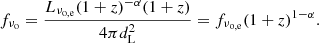
The fνo, e becomes
![$$ \begin{aligned} f_{\nu _{\rm o,e}} = f_{\nu ,\mathrm{o}}[(1+z)^{\alpha -1}], \end{aligned} $$](/articles/aa/full_html/2019/10/aa36270-19/aa36270-19-eq10.gif)
where the factor within square brackets is the K-correction. For the SDSS sources and the FIRST objects corresponding to an SDSS source we used α = 0.3, for the radio lobes we used α = 1 (0.3 is the most frequent value measured for the sources of our sample for which radio spectra are available in the Vollmer 2009 catalog Urry & Padovani 1995, and references therein). Finally, we calculated RK using the peak flux density at 1.4 GHz f1.4 GHz, P for CD sources and the integrated flux density at 1.4 GHz f1.4 GHz, I for FRII sources acquired from the FIRST catalog. Henceforth, we drop the P and I subscripts for f1.4 GHz keeping in mind that we use the peak flux density for CD objects and the integrated fluxes for FRII ones. It should be noted that in the case of FRII AGNs, the radio flux density is the flux density sum of all the radio components, core (if detected) and lobes.
3.2. Radio power and pseudo SFR
From the flux density at 1.4 GHz we calculated a formal estimate of the SFR (hereafter pseudo-SFR, pSFR) of each object following Yun et al. (2001):

with P1.4 GHz being the radio power at 1.4 GHz:

dL the luminosity distance in Mpc, and f1.4 GHz the flux density at 1.4 GHz in W/Hz.
The physical basis of the connection between radio emission and SFR is the synchrotron emission associated with supernova remnants. As the supernova remnants cooling times are relatively short, radio emission can be considered as a measure of instantaneous SFR. Computing a SFR from the radio power is certainly incorrect in the case of jetted RL sources. However, there are cases in which the radio power is relatively high, and in which the dominant contribution is not associated with the relativistic jet but, indirectly, to star formation processes (e.g., Caccianiga et al. 2015, who found that 75% of RL narrow-line Seyfert 1, NLSy1s, have Wide-field Infrared Survey Explorer, WISE, color indices consistent with star formation). We therefore compute the pSFR for all radio classes, being aware that this pSFR is not meaningful in the case of jetted RL sources. A term of comparison is offered by the SFR computed from the FIR luminosity (e.g., Calzetti 2013).
3.3. FIR power and K-correction
To obtain an estimate of the SFR from the IR luminosity we used the local calibration derived by Li et al. (2010):

with SFR70 μm in M⊙ yr−1 and L70 μm in erg/s, mostly derived from the Herschel flux density.
The observed flux needs to be K-corrected to obtain the rest-frame flux at 70 μm. The SED in the FIR can be represented by a single, modified black body:
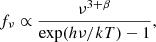
where h is the Planck constant, k the Boltzmann constant and T the dust temperature (Smith et al. 2014). We assume T ≈ 60 K because this is the temperature of the HII regions gas that correlates to the SFR in contrast with the galactic cirrus whose gas is at T ≈ 20 K and not connected to the SFR. The β term, referred to as emissivity index, modifies the classic Planck function with the assumption that the dust emissivity varies as a power law of frequency. We assume a constant β = 1.82 following Smith et al. (2014). Our goal is to get an estimate of the SFR for comparison with the pSFR derived from the radio power. The results can be found in Sect. 4.4. Even if a more consistent approach would have been the fitting of the IR SED with the various components emitting in the FIR spectral ranges, our estimates should be anyway fairly reliable because we expect that the main contributor to the flux at 70 μm, the dusty torus, has a steeply declining emission from a maximum at around 10–20 μm (Duras et al. 2017, and references therein)2. The K-correction (Eq. (3)) factor becomes:
![$$ \begin{aligned} K_{\rm FIR} = \left[ \frac{f_{\nu _{\rm e}}}{f_{\nu _{\rm o,e}}} (1+z) \right] = \frac{\nu _{\rm e}^{3+\beta }}{\nu _{70\mu \mathrm{m}}^{3+\beta }} \frac{\exp (h\nu _{70\mu \mathrm{m}}/kT)-1}{\exp (h\nu _{\rm e}/kT)-1} (1+z), \end{aligned} $$](/articles/aa/full_html/2019/10/aa36270-19/aa36270-19-eq15.gif)
where νe = νo(1 + z). The K correction in the FIR is of order unity for the seven sources listed in Table 5; all the observed fluxes are affected by a factor in the range ∼0.8 − 2.4.
3.4. Optical spectra analysis and derivation of physical parameters
The optical spectral study was done with the Image Reduction and Analysis Facility (IRAF)3. The first steps involved the conversion to rest-frame wavelength and the flux scale of the spectra, using the redshift values retrieved from the SDSS quasars catalog. Some sources show a different redshift with respect to that listed by the SDSS. In this case, a better estimate was calculated from the position of the [OII]λλ3726−3729 emission line doublet that provides a redshift identification that can minimize confusion with other single emission lines (Comparat et al. 2013; Bon et al., in prep.), or, if this doublet is not detected, from the Hβ narrow component position. An accurate rest frame definition is relevant to estimate a correct physical interpretation of internal broad and narrow line shifts, which are an important part of the results presented in this paper. After the z-correction, we normalized each spectrum to their continuum value at 5100 Å, that is, the mean over a region between 5050 and 5110 Å. Then, we measured the FWHM(Hβ) and its flux through a Gaussian fit of the emission line, and the Fe II blend flux by marking two continuum points at 4440 and 4680 Å and summing the pixels in this range, considering partial pixels at the ends. In this way we obtained an estimate of RFeII.
We computed the MBH of each source through the equation of Shen & Liu (2012) using the scaling parameters of Assef et al. (2011):
where a = 0.895, b = 0.520, c = 2.0, and  , in erg s−1 with dc being the radial comoving distance, λ = 5100 Å and fλ the continuum flux density at the quasar rest-frame. The λE follows from:
where L ≈ 10 L5100 is the bolometric luminosity and LE is the Eddington luminosity, the maximum luminosity allowed for objects powered by steady-state accretion (e.g., Netzer 2013). From the FWHM(Hβ) and RFeII values, we classified the objects in the E1 spectral types. Higher S/N composite spectra (compared to individual spectra) were computed as median composite spectra. The next step was the creation of a model, through a non-linear χ2 minimization procedure (in IRAF with the package specfit, Kriss 1994), fitting the composite spectrum of each class in the Hβ wavelength range from 4430 to 5450 Å. The models for Pop. A and Pop. B AGNs involve a similar number of components with the following constraints:
– Continuum was fit with a power-law for both populations.
– Balmer lines were fit in different ways based on the population of the source. For Pop. A objects, the Hβ line was fit with a Lorentzian profile, to account for the broad-component (BC), with a Gaussian profile, to account for the narrow-component (NC), and with a second Gaussian profile, called blueshifted component (BLUE), if needed, to account for a strong blue excess especially seen in sources with a high RFeII. For Pop. B objects, the line was fit with three Gaussian profiles, to account for the broad, narrow, and very-broad components (VBC). The broader VBC may be associated with a distinct emitting region referred as very BLR (e.g., Sulentic et al. 2000a; Snedden & Gaskell 2007; Wang & Li 2011).
– [O III]λλ4959,5007 doublet – For Pop. B sources, two Gaussian profiles were used to fit each doublet line, one to account for the blue excess of the line. For Pop. A objects, each doublet line was fit with three Gaussian profiles.
– The Fe II λ4570 emission was fit through a template based on I Zw 1 (Boroson & Green 1992; Marziani et al. 2003).
Finally, each E1 class composite spectrum was analyzed measuring the equivalent width (W), FWHM, and centroid shifts, c(x), of Hβ and [O III]λ5007 emission lines. The centroid shifts were defined as proposed by Zamfir et al. (2010):
where x is a specific height of the profile (we considered 1/4, 1/2 and 9/10), vr, R and vr, B refer respectively to the velocity shift on the red and blue wing in the rest-frame of the quasar. The interpretation of centroid shifts is mainly based on the Doppler effect due to gas motion with respect to the observer, along with selective obscuration (e.g., Marziani et al. 2016a; Negrete et al. 2018).
4. Results
Core-dominated sources are identified in Table A.1. Table A.1 reports SDSS identification, redshift, g band specific flux in mJy, peak flux density at 1.4 GHz in mJy, integrated flux density at 1.4 GHz in mJy if f1.4 GHz, I ≥ f1.4GHz, P, the decimal logarithm of log  , the decimal logarithm of L5100, the decimal logarithm of P1.4 GHz, the MS parameters FWHM Hβ and RFeII, along with a final classification code that includes radio-loudness class, radio morphology and optical ST. Borderline and intriguing cases of non-compact radio morphology are discussed in the footnotes of Table A.1. FRII required a careful identification following the method described in Sect. 3.1, with an a-posteriori vetting to exclude spurious features. Table A.2 identifies the optical nucleus and the radio features (lobes) that are not coincident with the optical nucleus for the FRII radio morphology. It provides, in the following order, the SDSS identification, the right ascension and declination of the optical core (Col. 2–3), right ascension, declination, and separation of the first radio lobe (Col. 4–6). The same information is repeated for the second radio feature in Col. 7–9. Column 10 provides the angle between the two lobes, with vertex on the nucleus, computed as described in Sect. 3.1. An Atlas of the FRII sources identified in this work is provided in Appendix A.
4.1. Trends along the MS
The numbers of sources in each MS spectral bin, for each radio-morphology class (CD, FRII), and for each radio-loudness emission range (RD, RI, RL) are reported in Table 1. There are a total of 38 RD, 139 RI and 178 RL objects.
Number of sources in each spectral type and radio-loudness range.
4.1.1. Source distribution along the MS
Table 1 shows that the most populated bins are the Pop. B ones, especially B1 and B1+ bins, at variance with the optically-selected sample in Fig. 1 where the most populated bins are B1 and A2. The occupation of the spectral bins decreases from type A1/A2 to A3/A4, with a fraction of A3+A4, ∼25% of the Pop. A (∼29% if A5 sources are included), a prevalence than the one measured on the optically-selected sample of Fig. 1: the A3+A4 fraction of Pop. A sources is ∼0.085/0.457 ≈ 19 %. The distribution of sources in the various STs depends on both radio loudness and radio morphology.
– Radio-detected sources are present only with a CD radio morphology. Population A and B are similar in number (21 A and 17 B) but Population B sources with a RFeII parameter higher than 0.5 are very rare (only three objects are in B2 and B3) in contrast with Population A objects.
– Radio-intermediate sources also are present only with a CD radio morphology. They are more numerous in Population B than in A (96 in B and 43 in A) in contrast to the RD class. However, xA bins are populated in a significant way by CD objects, and 63% of all the xA CD sources are RI.
– Radio-loud objects are more numerous in Population B for the CD radio morphology and they dominate in the FRII one (81 CD in B and 31 CD in A, all FRII in the sample are RL). RL (CD+FRII) in B1 and B1+ accounts for the wide majority of RL sources (2/3 of the total, Table 1). The FRII radio morphological class appears only in the RL domain in contrast with the CD one where all the three radio-loudness classes are significantly populated.
In summary, considering ST B1 and B1+, all FRII, and the wide majority of CDs (∼90%) are in the RI and RL ranges only. Moreover, FRII are a sizable number in ST B1 and B1+, but almost completely absent in Population A. Only three RL FRII sources appear in bin A1.
4.1.2. Hβ
Figures 3 and 4 shows the composite spectra fits, organized along the MS, for each radio morphology and loudness class. The spectra of the E1 classes (from left to right) confirm the systematic differences between Pop. A and B summarized in Sect. 1. Regarding the Hβ line profile, we note that Pop. A sources have a broad Hβ component best fit by a Lorentz function whereas the Pop. B ones are best fit with two Gaussians. This was expected and confirms results of previous studies as far as the Lorentzian profiles of the sources with the narrowest profiles are concerned (e.g., Véron-Cetty et al. 2001; Sulentic et al. 2002; Cracco et al. 2016).
 |
Fig. 3. Composite of STs along MS, ordered from B1++ to B2. Each panel shows the original composite, along with the modeled continuum (cyan line). The lower part of the panels shows the result of the specfit analysis on the emission lines. HβBC: black line, HβVBC: red line; Fe II: green line; yellow lines: Hβ narrow components and [O III]λλ4959,5007. |
In addition, looking at Pop. B sources, going towards higher values of FWHM(Hβ) we note that the peaks of the BC and VBC of Hβ become increasingly more separated. The trend is very clear passing from B1 to B1+ for CD RD and RI, as well as for FRII RL. Several physical processes could be at the origin of this effect: an infalling gas component, gravitational redshift, or a binary BLR associated with a binary black hole (BBH), with each BH giving rise to a single and distinct BC. These possibilities will be briefly discussed in Sect. 5.1.
Complementary information independent from line profile decomposition can be inferred from the lines centroid shifts and equivalent width behavior shown in Table 3 and in Figs. 5 for Hβ. Fig. 5 shows that in the CD class the value of c(9/10), c(1/2) and c(1/4) generally increases going from the Pop. A bins to the B1++. This translates in a redshifted line for Pop. B sources, more redshifted for larger FWHM(Hβ) values, and a slightly blue shifted or unshifted line for Pop. A sources. The only exception to this trend is CD RD B1+, with Hβ showing a small peak blueshift (c(0.9)≲ − 100 km s−1). Moreover, while in Pop. B bins W(Hβ) does not vary significantly, at the boundary between Pop. B and Pop. A W(Hβ) begins to decrease towards bins with higher RFeII, reaching a minimum in correspondence of ST A3.
 |
Fig. 5. CD Hβ centroid shifts (km s−1) for different E1 classes and for different line height. From top to bottom: x = 1/4, x = 1/2, x = 9/10. Bottom: equivalent width (Å) distribution. Blue refers to the RD class, green to the RI one, red to the RL one and black to the RL FRII class. |
4.1.3. [OIII]: equivalent width anti-correlation only for RD
The [O III] doublet becomes increasingly weaker in Pop. A going towards bins with higher RFeII values until the line almost disappears in A3 and A4 bins (Fig. 3, 4 and Fig. 6). This anti-correlation is one of the well-known and strongest trends of the quasar MS (Boroson & Green 1992; Boller et al. 1996; Sulentic et al. 2000b). However, only the RD class follows the anti-correlation, with the [O III] lines becoming indistinguishable from the FeII blend in the xA bins. RD sources behave, in this respect, similar to RQ sources. The W([O III]) of Pop. B composites does not vary strongly, whereas, after an increase in the A1 bin, the W([O III]) decreases going towards bins with higher RFeII. Fig. 7 shows that the W([O III]λ5007) behavior is somewhat different for the base semi-broad component and for the core component. The base component changes within a limited range of values (a factor ∼2 in the Pop. A ST for RL and RD composites that show W([O III]) in the range 3–7; a factor ∼5 in ST A2 and ∼2 in ST A1 for the CD RI); the core component, after a sudden jump for ST A1 that is less pronounced in the RD and RI classes with respect to the RL one, systematically decreases in all radio loudness classes. The core component is practically null from ST A3 in the RD class whereas in the RI and RL ones is still present. This creates the impression of a fairly constant [O III]λ5007 in RL (Fig. 4). The large W([O III] ≳10 Å) of the base component in spectral types B1+ and B1++ is apparently surprising, but the base component has a small shift with respect to the core component, so that the decomposition core/base is, in this case, ill-defined. The dependence on radio classes implies a significant strength of the NC among RL and RI CD compared to RD. This may be a genuine effect associated with radio loudness, not detected earlier because of the small number of RL if ST types are isolated along the sequence.
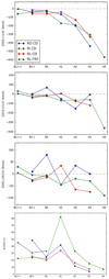 |
Fig. 6. CD [O III] centroid shifts (km/s) for different E1 classes and for different line height. From top to bottom: x = 1/4, x = 1/2, x = 9/10. Bottom: equivalent width (Å) distribution. Blue refers to the RD class, green to the RI one and red to the RL one. |
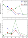 |
Fig. 7. Equivalent width of [O III]λ5007 as function of spectral types for CD RD, RI, RL sources. Upper panel: refers to the base, semi-broad component, the bottom one to the narrower core of the [O III]λ5007 line. |
Figure 6 shows that in the CD class the values of c(1/4) become increasingly negative from Pop. B to A, reflecting an increasing blueshift toward the line base. The blueshifting of the [O III] wing component, represented by c(1/4), is very common in AGNs but not every AGNs shows a fully blueshifted line, that is, a negative c(x) for all x. CD RL A2 and A3 show a systematic blueshift at 1/2 and 0.9 fractional intensity, although the blueshift amplitude is modest ∼100 km s−1. The most significant is the one of the RI A4 bin with the strongest Fe II.
4.2. Dependence on radio classes for a fixed spectral type and/or population
4.2.1. Hβ
Interesting findings can be seen by comparing the different radio-loudness emission classes within each ST or at least in Pop. A and B. Generally speaking, for all STs, going from the RD to the RL class, the line shape and intensity do not vary significantly, as can be seen from the spectra in Figs. 3 and 4. The Pop. B Hβ profiles are always Gaussian-like. Pop. A Hβ profiles can be well-fit by a Lorentzian function independently from radio class. In all STs, the Fe II template reproduces equally well the Fe II emission across all radio classes, within the limits in S/N and dispersion. An important inference is that the properties of the low-ionization BLR emitting most of Hβ are little affected by radio loudness.
Pop. A. In bin A1, the Hβ line profiles are intrinsically symmetric independently on radio loudness (Table 3), and the apparent redward excess can be explained by the combined effect of optical Fe II blends and [O III]λλ4959,5007 semi-broad emission. Modest shifts to the blue appear in bin A2, and are apparently stronger for RL CD. In the A3 bin, both the RD and RI Hβ profiles show a blueshift. A blue shifted excess for Hβ in the RL CD A3 composite is reflected by the increase in blueshift amplitude toward the line base. The RI CD A4 Hβ profile is also consistent with a blueshifted excess toward the line base (Fig. 4), although the line peak for all radio classes and ST remains unshifted.
Pop. B. From Fig. 5 we note that line centroids do not vary qualitatively in the different CD radio-loudness classes with the exception of the B1+ bin where the RD class shows a Hβ profile redshifted at the base and at half height and slightly blueshifted at the peak. Radio detected, RI and RL show a prominent red wing, as can be seen in Fig. 8 where the profiles of Hβ for the CD B1 radio classes are shown. The redward displacement of c(1/4) is maximum for ST B1 for RL CD and for RD CD B1+. In the FRII class, whose objects mostly belong to Pop. B, the Hβ line is redshifted in all composites (Fig. 5). The redshift increases with increasing FWHM(Hβ), as also found for the CD radio morphology.
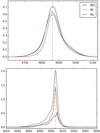 |
Fig. 8. CD B1 Hβ (top) and CD A2 [O III] profiles (bottom) for different radio power classes. Blue refers to the RD class, green to the RI one and red to the RL one. |
4.2.2. [OIII]λλ4959,5007
Pop. A. The [O III]λλ4959,5007 lines are usually asymmetric in correspondence of the line base, from the A1 to the xA bins. The [O III]λ5007 line is slightly blueshifted and asymmetric in ST A1 if RD and RI classes are considered. Table 3 reports a small blueshift ∼ − 50 km s−1 that apparently disappears for the CD RL class ST A1, the only case where the [O III]λ5007 profile it is perfectly symmetric. The blueward asymmetry of the ST A2 and A3 composite [O III]λ5007 profiles is instead large due to centroid at 1/4 shifts of ∼400 km s−1 for the three radio classes (Table 3 and Fig. 6).
Sources that shows a blueshift higher than 250 km s−1 at peak have been termed blue outliers and are common in the xA class (Zamanov et al. 2002; Komossa et al. 2008; Negrete et al. 2018). In the xA bins almost the whole line is blueshifted, although the blueshift is modest at peak and none of the composite spectra would qualify as a blue outlier following Zamanov et al. (2002): shifts are large close to the line base (≲ − 300 km s−1) but tend to 0 or to a small blueshift value in correspondence of the line peak. In A2 and A3 there might be a trend as a function of the radio class as far as the amplitude of the [O III]λ5007 blueshift close to line peak is concerned (Fig. 4), with the [O III]λ5007 peak blueshift increasing from RD to RL, but with a shift amplitude < 100 km s−1. Only RI CD A4 comes close to a blue outlier (c(1/4)≈ − 600 km s−1, c(1/2) ≈ − 350 km s−1, c(1/4)≈ − 100 km s−1) below the conventional limit of −250 km s−1 at the peak, which may imply that some of the sources of this ST are indeed blue outliers. The RI CD A4 sources are listed in Table 2 that identifies all the xA sources of the sample and provides their classification. A study of individual spectra is required, as the sources listed in Table 2 with classification CD RI A4 should be considered blue outlier candidates.
Extreme Population A sources.
In the present sample, the [O III]λ5007 blueshift at quarter maximum is only slightly larger in RD than in RI and RL for ST A3 and A4. The shift and to some extent the equivalent width of base component in [O III] is not strongly dependent on the radio class. Especially at 1/4 fractional intensity the shifts remain relatively high amplitude due to an appreciable semibroad component. (Table 3 and Fig. 4). This behavior is at variance with the one observed in the [O III]λλ4959,5007 lines in Pop. B, as far as the amplitude of the shifts is concerned. In Pop. B, we observe a slight increase of the blueshifts toward the line bases, but the amplitude is ≲100 km s−1. It is interesting to note that, for the resonance high ionization C IV λ1549 line (whose blueshift is related to [O III]λ5007 (e.g., Coatman et al. 2019, and references therein), RL samples show systematically lower blueshift amplitudes than RQ (Richards et al. 2011; Marziani et al. 2016b). A possible interpretation resides in the interplay between the accretion disk wind and the relativistic jet, with the latter hampering the development of a high-speed wind.
Hβ and [O III] properties of each spectral type, radio-power and radio morphology class.
Berton et al. (2016) found that RL NLSy1s show more prominent [O III]λ5007 blueward displacements than RQ ones. Considering that NLSy1s show the narrowest Hβ profiles among Population A (and are completely absent by definition in bin B1 where the powerful jetted CDs are found), their results is not necessarily in contradiction with ours, as large amplitude shifts close to line base are also found in our sample of RI and RL CDs. The issue is whether the sources in our sample could be assimilated to the RL Pop. A of Berton et al. (2016). Unfortunately only 1 source out of 61 is in common, SDSSJ135845.38+265808.4, from the Foschini et al. (2015) sample of flat-spectrum NLSy1s. Its classification is CD RI A2, shows a Lorentzian Hβ broad profile, and relatively strong [O III]λλ4959,5007. The [O III]λ5007 line has a prominent semi-broad component, whose shift (tentatively measured on the DR12 Science Archive Server) is ∼ − 1000 km s−1. The properties are consistent with the properties of RQ sources in this spectral bin, and are akin to the xA RI. The WISE color index W3 − W4 > 2.5 indicates the presence of a starburst component (Caccianiga et al. 2015), suggesting a thermal origin for the radio power (Sect. 4.4).
Pop. B. The [O III]λ5007 line can be considered almost symmetric and unshifted all across the radio classes in Pop. B for both CD and FRII classes; the trend of an increase in blueshift toward the line base is preserved although Table 3 reveals that now the shifts at the line base are ≳ − 100 km s−1. In other words, CD RQ, RL and RI Pop. B show a similar behavior at 1/4 maximum, with a modest blueshift, and no significant shift at peak.
4.3. Relation to physical parameters
Table 4 reports several physical parameters for each E1 ST related to radio power and radio-morphology class: L5100, MBH, λE, P1.4 GHz, log  , and pSFRr. The reported values are the median of the parameters of all the sources belonging in a given E1, radio-morphology and radio-power class.
Physical parameters of each E1, radio power and radio morphology class.
Following the E1 trend from the B1++ to the A4 ST, there is an increase of λE and a decrease of the MBH, in agreement with past works (e.g., Fraix-Burnet et al. 2017, and references therein). Populations A and B as a whole also show difference in terms of the MBH and λE, with Population B showing more massive BH having a lower λE with respect to the Population A. The systematic difference in λE and MBH are likely to account for the trends along the E1 MS (e.g., Sun & Shen 2015). Around the critical value of λE ≈ 0.2 ± 0.1 the active nucleus may undergo a fundamental change in accretion mode and BLR structure (Wang et al. 2014).
Focusing the attention on the different radio-loudness classes, MBH and the λE do not vary greatly along the radio classes: the B1 ST involves MBH ≈ 109 M⊙, whereas the A2 ST MBH ≈ 108 M⊙ along all radio classes. The trends related to RL appear to be “orthogonal” with respect to the E1 MS trends concerning the low-ionization part of the BLR. The MBH and λE values are, on average, comparable in each ST for the different radio classes. Differences in each ST for different radio classes described earlier might have been lost in large samples of AGNs including RQ and RL quasars because RL quasars are a minority.
4.4. Radio and FIR SFR
Table 5 lists SDSS identification and properties of seven objects of the sample considered in the present paper for which FIR data are available. The properties listed are, in the following order: the SDSS ID, the radio and FIR specific flux densities, radio power at 20 cm, the luminosity at 70 μm or 100 μm, the SFR(FIR), the pSFR from the radio power, and the classification code. Since only seven sources are found to have available FIR data to be used for the Bonzini et al. (2015), we considered additional samples to ease their interpretation: the union of the low-zSani et al. (2010), and Marziani et al. (2003) samples, along with the sample of Marziani & Sulentic (2014). A search in the NASA/IPAC Infrared Science Archive (IRSA)4 for Herschel, Infrared Astronomical Satellite and Spitzer data at 70, 100, and 160 μm yields 73 sources in total: seven from the present work, three from Marziani & Sulentic (2014), and 63 from the joint Sani et al. (2010), and Marziani et al. (2003) papers. The samples were vetted to preferentially select Pop. A and especially xA ST, although some well-studied Pop. B quasars were included.
FIR and radio data.
Following the FIR-radio correlation for star forming galaxies and quasars as shown by Bonzini et al. (2015), we assume that the maximum possible SFR is SFRmax = few 103 M⊙ yr−1. The SFR is ≲6000 M⊙ yr−1 in the most luminous sub-mm galaxies, with a turn-down at ∼2000 M⊙ yr−1 (Barger et al. 2014). Higher SFR are most likely unphysical, since the feedback effect due to stellar winds and supernova explosions may bring star formation to a halt on a short timescale.
The goal is to gain information about the dominating process in the radio AGNs activity, that is, to distinguish between star formation or relativistic jet even if we cannot exclude that, in any class we identified, there is a contribution from the non-thermal activity of the nucleus. The shaded area in Fig. 9 delimits the region of star forming galaxies and of RQ quasars. Comparing the radio and FIR SFR shows that five out of seven sources of the sample presented in this work fall in the region of RQ quasars, including two RL and three RD. None of the sources that fall in the RL region (outside the shaded area in Fig. 9) is an xA source.
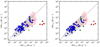 |
Fig. 9. FIR luminosity vs. radio power. The shaded areas trace the occupation zone of star-forming galaxies (gray) and RQ quasars (pink) following Bonzini et al. (2015). Color codes are: red (RL), green (RI), blue (RD). Left: sources identified on the basis of spectral types; xA: circled symbols; A2: circles; A1: pentagons; B1: squares; B2: rhomboids; not defined: open symbols. Right: sources identified on the basis of samples. Circles: this work; rhomboids: Marziani & Sulentic 2014, squares: Sani et al. 2010 + Marziani et al. 2003. |
The left panel of Fig. 9 identifies the ST of the 73 sources. The most luminous xA sources can reach ∼1039 erg s−1 Hz−1 (comparable to powerful RL jetted sources), although low-z xA sources understandably populate the lower part of the RQ zone. However, of the ten RQ sources above SFR∼ few 100 M⊙ yr−1, five are xA, two borderline xA (A2 with RFeII slightly below 1), one B1, one A1, and one has no defined ST due to poor data. Therefore, the majority of sources at the highest radio powers and SFR shown in Fig. 9 are apparently xA, and their placement in the Bonzini et al. (2015) diagram is consistent with them being RQ.
xA sources are mainly classified as RD. The xA sources are predominantly blueish quasars, as testified by their high prevalence in the PG survey. Several of them are also borderline RI with log RK slightly below 1. Had they been affected by some internal extinction, they would have been classified as RI. Far-infrared data for CD RL A3 and A4 of our sample are unfortunately missing. The only xA source classified as RI is Mark 231, a high-L, low-z broad-absorption line quasi-stellar object suffering some internal extinction (Sulentic et al. 2006; Veilleux et al. 2016). Mark 231 has been described by Sulentic & Veilleux and collaborators as a prototypical high-L, highly accreting quasar placed at low-z. Extreme Pop. A properties are extreme in terms of Fe II emission, C IV λ1549 blueshift, and blueward asymmetry of Hβ. Mark 231 is known to possess an unresolved core, highly variable and of high brightness temperature (Condon et al. 1991). Superluminal radio components of Mark 231 have been detected, and the relation between broad-absorption lines, radio ejections, and continuum change (Reynolds et al. 2017) illustrate the complex interplay of thermal/nonthermal nuclear emission that can be perhaps typical of xA sources. Still, according to the location in the diagram of Fig. 9, the dominant emission mechanism is thermal. This inference is consistent with the enormous CO luminosity of the AGN host (Rigopoulou et al. 1996).
5. Discussion
Our sample sources follows the MS, and in Sects. 5.1 and 5.2 we discuss the Hβ and [O III] trends with reference to the radio class. We want to stress again that the distribution of sources in the various STs is different from the one of optically-selected samples mainly consisting of RQ sources, and depends on both radio loudness and radio morphology (Table 1). As mentioned, the majority of objects in the present sample belong to the B1 and B1+ bins, whereas the number of sources goes down in bins with higher FWHM(Hβ), such as B1++, and higher RFeII, that is, toward Pop A2 ST and onward. The highest values of the radio power are seen in Pop. B for FRII and CD objects. All these objects are most likely jetted RL quasars. The Hβ FWHM may be lower than the Pop. A upper limit if the CD are FRII sources seen at relatively small viewing angles (Sect. 5.4). On the converse, broadest profiles (bin B1++) may indicate a favorable orientation for the detection of a double structure, possibly associated with sub-pc supermassive BBHs (Sect. 5.5).
The CD class exhibits a significant number of xA sources, ∼30% of all Pop. A are CD objects. Interestingly, ∼18% of xA CD AGNs have a radio power emission in the loud range, a prevalence even higher than the prevalence of RL sources in optically-selected samples. The high prevalence in sources whose appearance is “very thermal” in the optical and UV ranges (Negrete et al. 2018; Martínez-Aldama et al. 2018) calls into question the origin of their radio power (Sect. 5.6).
5.1. Spectroscopic trends: Hβ
The radial velocity dispersion (in the following δvobs = FWHM) can be written as
where κ = δviso/δvK, the ratio between an isotropic δviso and the true Keplerian velocity δvK. κ ≈ 0.1 ≪ 1 implies a highly-flattened configuration, and a strong dependence on the line width of the viewing angle θ. The effect of the viewing angle appears to be most important in the low-RFeII region of the MS (i.e., STs B1+, B1 and A1), and will be discussed with reference to the RL FRII/CD relation (Sect. 5.4).
Orientation effects ideally leave a symmetric profile. The Hβ line however shows systematic trends of asymmetry and centroid shifts along the MS: in Pop. A, from A2 to A4, blueshifts become more prominent, such as the case of [O III]λλ4959,5007. The physical basis of the blueshift is most likely Doppler-shifted emission by outflowing gas approaching the observer, with the receding side of the outflow hidden from view (Marziani et al. 2016a, and references therein).
The prominence of the outflow is related to the λE, which is believed to increase with increasing RFeII along the sequence (e.g., Grupe et al. 1999; Sun & Shen 2015; Du et al. 2016a; Sulentic et al. 2017). The frequency of detection of a blue shifted excess over the symmetric Lorentzian profile assumed for Pop. A, is 0 in A1, very low in A2 (the blue excess is detected rarely), sizeable in A3, and high in A4.
Extreme Pop. A sources are the ones expected to provide the maximum feedback effect on the host galaxy. In other words, they are the AGNs most likely to affect the dynamical and structural properties of the host, and may be ultimately lead to the well-known correlation between MBH and bulge mass (e.g., Magorrian et al. 1998; King & Pounds 2015, and references therein). Radio observation offer an unobscured view of star formation, and can be directly compared to FIR measurements (which are, at present, available only for a small subset of our sample). This may have profound consequences in our understanding of galaxy evolution, as a proper estimate of the SFR at high redshift and for sources fainter than the ones considered in this analysis may allow to analyze to which extent feedback effects may be produced by the AGN itself or by induced star formation.
On the converse, in Pop. B, the Hβ profile appears predominantly redward asymmetric toward the line base. The asymmetry affects the FWHM by about 20% (Marziani et al. 2013, and references therein). There is ample evidence that the Pop. B Hβ broadening is dominated by virial motions. However, the origin of the redward asymmetry is unclear. Two main possibilities are considered: infall (+obscuration) and gravitational redshift. It is at least conceivable that some line emitting gas is drifting toward the central BH at a fraction f of the free fall velocity (e.g., Wang et al. 2017). In this case, the centroid displacement can be  . The real difficulty in this scenario is to envisage a dynamical configuration that allows for a steady inflow with the receding part hidden from view in a large fraction of quasars. The alternative mechanism is gravitational + transverse redshift (e.g., Bon et al. 2015, and references therein). In this case, the net effect is expected to be a line shift by
  , where zg = GMBH/c2rBLR, with rBLR being the BLR size. The centroid displacement should be
  , independent on orientation. The problems with gravitational redshift stem from the compactness of the emitting region that is required to produce a shift as large as 2000 − 3000 km s−1. The issue is open at the time of writing but the relevant result of the present paper is that all radio classes show a prominent redward asymmetry. Redward asymmetries were revealed as a systemic properties of the Hβ profiles of Pop. B RQ quasars (Marziani et al. 2013) and in RL alike (Punsly 2010). The implication is that this feature is unlikely to be a consequence of the jetted nature of RL sources.
5.2. Spectroscopic trends: [OIII]
In typical SDSS spectra, the [O III] profile can be well-represented by two components: a narrower one and a blueshifted semibroad “base” component (e.g., Komossa et al. 2008; Zhang et al. 2011; Marziani et al. 2016a). The relative intensity of the two components is dependent on the ST along the MS. The presence of blueshifts and blue asymmetries among RL and RI indicates emission of [O III]λλ4959,5007 by outflowing gas, in analogy to the cases of the RD class in this sample, and of the broader RQ class in previously-analyzed samples (e.g., Zamanov et al. 2002; Bian et al. 2005; Komossa et al. 2008; Zakamska et al. 2016, the RD sample is at the high end of the RQ class radio emission). The fairly constant value of the W([O III]λ5007) base component has been found also in previous investigations spanning a wide range in luminosity (Marziani et al. 2016a). The proportionality between continuum and line luminosity then supports a nuclear origin for the blueshifted line component.
5.3. Radio power and radio loudness
5.3.1. Population A and B intrinsic differences
FRII sources are the parent population of all powerful RL jetted AGNs (Urry & Padovani 1995). Radio-loud FRII have typical Pν ≈ 1026 W Hz−1, and Pop. B CD RI and RL share similar Pν values with them in bin B1+. Population B CD RI show a lower Pν than RL, but, even if lower, the RI CD sources show radio powers that are systematically higher than the RI CD sources in Population A, at least by a factor of several. The radio power values reported in Table 4 and the distribution of radio powers for RL and RI for the STs along the MS (Fig. 10) show that, although there is a considerable overlap, the distributions of the xA Pν is significantly different from the one of the Pop. B sources, for both RI and RL: a Kolmogorov-Smirnov test yields PKS ≈ 0.01 for the RI, and PKS ≈ 0.004 for RL. The behavior of the Pν vs.  for the various STs (Fig. 11) adds further evidence in favor of an intrinsic difference between the two populations: Pop. B sources of the three radio loudness classes are significantly correlated, with a unweighted least square fit yielding
  . The trend is much shallower for the xA sources and the slope of the best-fit is not significantly different from 0log Pν ≈ (0.136 ± 0.168)log RK′ + (24.261 ± 0.246). The Pop. B relation is consistent with the idea that all sources owe their radio power to the same mechanism: specifically, we expect that jetted sources are exclusively synchrotron radiation in the radio, and that the synchrotron emission is also giving an important contribution in the optical. On the converse, the xA sources show a large Pν scatter for a given
  .
.
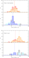 |
Fig. 10. Distribution of radio power Pν in units of W for RI (top) and RL (bottom), for different spectral types along MS. Top panels: distributions for the union of B1++ and B1+ (red), B1 (orange) spectral types, the bottom ones for A1 (gray), pale blue (A2), and xA (blue). The vertical dot-dashed lines mark the medians of the Pop. B (red and orange), A2 (pale blue) and xA (blue) distributions. |
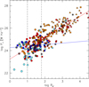 |
Fig. 11. Behavior of radio power Pν in units of W as function of Kellermann’s parameter |

In addition, there is a significant range of FIR luminosity for a given radio power (∼1 order of magnitude, Fig. 9). The origin of the range in optical and FIR properties for the xA remains to be clarified. While extinction could be at the origin of the dispersion in  , the FIR range for a given Pν instead suggests a spread in the star formation properties of the host galaxy.
5.3.2. Kellermann’s parameter as an identifier of RL sources
Figure 12 shows the  index distribution for FRII, Pop. A and B CD sources. The FRII distribution validates the limit at log
  suggested by Zamfir et al. (2008) who proposed the minimum FRII
  to identify jetted sources. Albeit simple, this limit may not be applicable to CDs. The basic reason is that lobes are due to extended emission representing emission integrated over the history of the activity cycle, whereas measurement of the core are “instantaneous” (e.g., De Young 2002, and references therein). The distribution of CD Pop. B (middle panel of Fig. 12) shows that CD are mainly distributed with log
  , which instead suggests a validation of the classical condition. The continuous distribution of radio powers (Fig. 10) indicates that it is perhaps not meaningful to look for a bimodal distribution. Even if this sort of distribution is sometime seen (e.g., Gupta et al. 2018), the appearance may be dependent on selection effects involving frequency and selection criteria (La Franca et al. 2010; Cirasuolo et al. 2003). For instance, Fig. 12 suggests a bimodal distribution if RL FRII and Pop. B CD are merged. The implication is that jetted sources might be associated with log
  . However, in Pop. B truly jetted sources are found in the range
 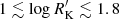 .
.
 |
Fig. 12. Behavior of log |

The limit log RK ≳ 2.4 proposed by Falcke et al. (1996) would give rise to a bimodal distribution of log RK for CD Pop. B sources implying that among CD only a relatively small fraction could be truly jetted. In relatively old samples RL sources were confined to very massive BHs. These samples even suggested a MBH “threshold” for radio loudness (see the recent analysis of][and references therein Fraix-Burnet et al. 2017). This view might have become outdated because of the discovery of RL NLSy1s (Komossa et al. 2006), and because of systematic comparisons between MBH in RL and RQ samples (Woo & Urry 2002). Results support the presence of jetted sources with small MBH, with RL sources spanning a broad range of masses. While the CD Pop. B sources with log RK ≳ 2.4 could be likely considered the “face-on” counterpart of the FRII in our sample, low MBH RL Pop. B sources could be jetted as well, since the power of a radio jet depends on three factors: MBH, the magnetic field intensity, and the spin angular momentum of the BH (Blandford & Znajek 1977). Classical FRII along with the FRII identified in this work are extended sources, whose ages are estimated around several hundreds of million years (e.g., Ito et al. 2006). The lobe extension has an evolutionary meaning akin to MBH that can only grow over cosmic time (Fraix-Burnet et al. 2017). So, whether the  distribution may appear unimodal or bimodal may depend on the MBH distribution of the sample.
FRII sources do not include RD and RI objects in contrast to the CD class. They show a small prevalence in Population A, limited exclusively to ST A1. The existence of Pop. A FRII objects may be explained in term of the angle between the line of sight and the radio axis, as discussed below (Sect. 5.4). The same effect is expected to operate also for RI and RL CD in Pop. B. The largest  in ST A1 and A2 might be similarly ascribed to sources seen preferentially face-on. The high radio power that implies extremely large pSFR, and the consistency with the expectation of unification models for RL sources, make it unquestionable to consider both RI CD along with RL CD as jetted sources, and the condition
  sufficient to identify truly jetted sources in Population B and in bin A1. Considering the radio power of the CD RD B1+ that is comparable to the one of CD RI B1+ (Table 4), it is even possible that some sources at RD loudness level belonging to Pop. B might be intrinsically jetted. For the remaining ST of Population A, the situation is expected to be fundamentally different (Sect. 5.6), although in the samples used for Fig. 9 we have no indication of thermal xA sources entering into the RL radio-loudness range, and thus no direct evidence that the condition log RK ≳ 1 does not select truly jetted sources.
5.4. Orientation effects among RL sources
The existence of the A1 FRII sources may be explained in term of the angle between the radio axis and the line of sight. In this view, they should be simply end-on extended double sources with a Doppler-boosted core (e.g., Blandford & Rees 1978; De Young 1984). To better understand this effect, Wills & Browne (1986) investigated how the FWHM(Hβ) changes as a function of a parameter Rc, the ratio between the radio flux density of the core and that of the extended lobes. The parameter Rc reflects the angle between the radio axis and the line of sight in the relativistic beaming model for radio sources. The top plot of Fig. 13 shows a continuous distribution in both Rc and FWHM(Hβ) that goes against the idea of two distinct classes characterized by a flat and a steep spectrum. Instead, the trend may translate into an intrinsic difference between sources with high and low Rc values or, if relativistic beaming models are correct, it may translate in a different viewing angle of the emission line regions. In this case, the motions of the emission-line gas would be predominantly in a plane perpendicular to the radio axis. Then, the gas velocity field can be expressed as in Eq. (14). In the top plot of Fig. 13 the relation between observed Hβ FWHM and Rc is showed by the magenta line, for viso = 4000 km s−1, vp = 13 000 km s−1. The beaming model discussed by Orr & Browne (1982) is used to relate θ and Rc as:
![$$ \begin{aligned} \cos \theta =\dfrac{1}{\beta } \left\langle \dfrac{1}{2R_{\rm c}} \left\{ 2R_{\rm c}+R_{T}-[R_{T}(8R_{\rm c}+R_{T})]^{1/2} \right\} \right\rangle ^{1/2}, \end{aligned} $$](/articles/aa/full_html/2019/10/aa36270-19/aa36270-19-eq41.gif)
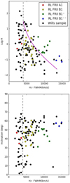 |
Fig. 13. Top: core-to-lobe radio flux density ratio vs. FWHM(Hβ), adapted from Wills & Browne (1986). Colored dots represent sources of our sample: red dots represent A1 RL FRII sources, yellow dots B1 RL FRII, green B1+ RL FRII and blue ones B1++ RL FRII. Black dots are the original data from Wills & Browne (1986). The magenta line represents the change of R with FWHM(β), predicted by the Orr & Browne (1982) beaming model with RT = 0.024 and γ = 5. Bottom: FWHM(β) vs. inclination, derived from Rc through Eq. (16). |
where RT = Rc(90 ° ) and β = v/c. Sources of the present samples are shown by red circles (A1 FRII), yellow (B1 FRII), green (B1+) and blue (B1++) whereas black circles refer to the Wills & Browne (1986) sample. Our sources follow the trend as the ones of Wills & Browne (1986). On average, the narrower FRII A1 sources have a higher Rc, whereas the broader B1, B1+ and B1++ sources have lower values suggesting that the orientation is an important factor affecting the line width. The bottom plot of Fig. 13 shows the trend between the FWHM(Hβ) and the inclination estimated following the work of Marin & Antonucci (2016) through the equation:

where LRc = log(R5 GHz), g = 41.799 ± 1.190, h = −20.002 ± 1.429, j = −4.603 ± 1.347, k = 0.706 ± 0.608, l = 0.663 ± 0.226, m = 0.062 ± 0.075. The range of inclinations a source can have gets smaller going towards higher FWHM(β) (sources with FWHM(Hβ)≳7000 km s−1 are constrained by θ ≳ 50°), but no source shows an inclination higher than ∼70° and only sources with FWHM(Hβ)≲7000 km s−1 show an inclination smaller than ∼40°. There is no restriction on θ at low FWHM(Hβ); highly inclined source can be Pop. A, implying that the viewing angle, although important, is not the sole factor affecting the Hβ width. The inclination values for the three FRII RL A1 in our sample are intermediate (35 ≲ θ ≲ 45 degrees), that is, located in the lower part of the θ vs. FWHM(Hβ) diagram (Fig. 13) where orientation effects are expected to be relevant. We conclude that the FRII RL sources, the parent population of all jetted sources, is confined in Pop. B but these sources seen at smaller viewing angle may enter ST A1. Considering that the probability of observing a source at angle θ in an idealized sample of randomly-oriented sources is ∝sinθ, ST A1 is expected to be infrequently occupied by truly jetted sources of radio classes RL FRII and RL CD. Actually, a non-negligible occupation in A1 from RL CD occurs because real radio flux-limited sample are biased in favor of smaller viewing angle due to relativistic beaming. As a matter of fact, flux-limited, optical samples of quasars contain a large fraction of their RL population that are flat-spectrum radio sources (Falcke et al. 1996).
5.5. Candidate binary black hole systems in extreme Population B
Super-massive binary black holes (SMBBHs) are thought to be produced during the merging of two galaxies. Their detection and number estimates can give us constraints on formation and evolution of galaxies (Hopkins et al. 2006). The presence of a BBH in the nucleus of a RL AGN was first suggested by Begelman et al. (1980). Super-massive BBHs may lead to an increase of the AGN activity and trigger starburst processes (Gaskell 1985). More important to our topic, ideas have been proposed that see the formation of radio jets associated with the merger of a BBHs (Wilson & Colbert 1995). Binary BHs are thought to be a possible cause of the different classes of RL AGNs and of the misalignments between the direction of radio jet and the accretion disk (Merritt & Ekers 2002). In addition to these effects the presence of two BHs may affect the dynamics of the BLR gas marking the profiles of the emission lines (Begelman et al. 1980), creating in some cases highly-shifted single-peaked emission lines (BBH “Doppler” detection). Then from the broad optical lines stems a way to detect BBHs system with sub-parsec separation (e.g., Bon et al. 2012; Li et al. 2016).
Looking at at the composite spectra shown in Fig. 3, we note that several Hβ profiles in Pop. B could reflect this situation. Especially striking appear the cases of RD CD B1+ (where a significantly blueward-displaced HβBC provides the best fit), RI CD B1+, RL CD B1+, RL FRII B1+ and FRII RL B1++. The Hβ profile includes a component close to the rest frame, but slightly displaced toward the blue, and a component with a larger displacement to the red. This configuration is consistent with the expectation of two BLRs, one associated with a more massive BH (the less-shifted component) and one associated with a less massive BH orbiting around a common center of mass. However, the blue shifted peak may be also due to an unresolved outflow.
We tested the conventional model BC+VBC (symmetric or slightly redshifted BC and redshifted broader VBC) of the Hβ profile with a BC+BC model, in which one BC is significantly blueshifted and one is significantly redshifted. We considered cases in which the BC+VBC model fit yielded a blueshift for the BC. Four cases are shown in Fig. 14. In the case of CD RD B1+, the BC+BC model was tested against a BC+VBC model fit in which the peak of the BC was set to 0. Table 6 reports the results of an F-test between the two models, listing in the following order the ST identification, the fitting model, the standard deviation, the χ2, the ratio F and the probability of a chance occurence for values of F lower or equal than the observed one. The BC+BC fit is significantly better for RD CD B1+ and RL CD B1+, whereas there is almost no difference for CD RI B1+. The BC+BC model for FRII RL B1++ is apparently worse than the VBC+BC one although the difference is not significant. In this latter case, indications in support of a binary BLR are provided by the analysis of the individual spectra. Inspection of the eight RL FRII B1++ Hβ profiles shows that, along with redward asymmetries or bumps, objects show symmetric and blue bumps or strong blueward asymmetries. This is the configuration naively expected in a sample in which a second feature radial velocity displacement is due to rotational motion around a more massive BH that roughly sets the center of mass of the binary system. B1++ are believed to be massive or highly inclined sources that maximize the orbital velocity projection along the line of sight (e.g., Panda et al. 2019). This is part of the evidence suggesting that RL sources might be preferentially associated with SMBBHs, although the observation of single-epoch profiles and even extended temporal monitoring usually do not exclude other phenomena connected with accretion disk instabilities (e.g., Storchi-Bergmann et al. 2017, and references therein). Sources in the B1++ ST are high-MBH, low λE accretors. Relatively low accretion rate is known to be associated with extreme variability (even at a “changing look” level, Noda & Done 2018), giving rise to complex emission line profiles.
 |
Fig. 14. Comparison between broad + very broad and double broad Hβ fitting models. From left to right, top to bottom: CD-RD-B1+, CD-RI-B1+, CD-RL-B1+ and FRII-RL-B1++. For each pair the left plot represents the broad + very broad fitting BC+VBC model and the right plot represents the double broad component model BC+BD. Color scheme same as in Fig. 3. |
Fitting model parameters and F test.
While it is obviously not possible to demonstrate the presence of a sub-pc BBH even in the cases where a double BC provides a better fit than the fit BC+VBC, our analysis identified STs with a higher prevalence of profiles that suggest possible SMBBH candidates. This means that Pop. A sources (which are always almost unshifted and symmetric) might be excluded in a systematic search for SMBBH candidates.
5.6. Interpretation of the radio pseudo-SFR
The origin of radio emission in RQ quasars is still debated (e.g., Panessa et al. 2019, and references therein). Star formation is considered an important agent especially at lower power (the fraction of star-forming galaxies is increasing at fluxes below 10 mJy Condon 1989), although other mechanisms more closely related to the AGN have been proposed.
An important result of the present investigation is the identification of the population of RI and RL sources in ST A2, A3 and A4. A3 and A4, or in other words xA sources, that are known to have high accretion rate, possibly at a super-Eddington level (Du et al. 2016b). High λE (and the defining property of xA sources, RFeII ≳ 1) can coexist with powerful jetted radio emission (log Pν ≳ 1031 erg s−1 Hz−1, in the power ranges of the Population A sources). There is no physical impossibility in this respect (Czerny et al. 2018, and references therein), and recent works consider the relativisitic jet and non-relativistic wide angle outflows as two aspects of an hydromagnetically-driven wind (Reynolds et al. 2017). Concomitant high accretion and high radio power are observed in CSS (Wu 2009; Sulentic et al. 2015). Our view is likely biased by the relative rarity of this sort of sources at low-z (O’Dea 1998), and especially by the scarcity of high-quality optical and UV spectra. The estimates of pSFRs derived from the radio power should be interpreted carefully. The basic issue is whether the RL and RI in the xA spectral bins are truly jetted Pop. A (as RL NLSy1s are believed to be) or dominated by thermal emission in their radio power.
Since RL jetted sources are expected to have FIR luminosity much below the one expected for their radio power if they were following the RQ FIR-radio relation, they are preferentially excluded from the Bonzini et al. diagram. This is expected to occur also for the RL xA Pop. A of the present sample. On the one hand, the trend shown in Fig. 9 (all xA in agreement with the RQ correlation) suggests that RL and RI xA, that are sources with power comparable with the ones of RI and RD (≳1031 erg s−1 Hz−1), may be intrinsically RQ and with power due to thermal process. Even if they are intrinsically rare sources, thermal sources emitting Pν ≳ 1031 erg s−1 Hz−1 are found in the local Universe (Condon 1989). The increase in prevalence of RL Pop. A objects after a deep minimum in correspondence of ST A2 calls into question the notion that the origin of the radio power in ST A3 and A4 might be necessarily the same of the jetted sources of Pop. B. On the other hand, RL NLSy1s do exist, and may show significant FeII emission. They may be showing a large blueshift in the [O III]λλ4959,5007 profiles (Berton et al. 2016; Komossa et al. 2018). therefore RL NLSy1s may appear undistinguishable in the Hβ spectral range from their RQ counterparts. The radio power may be associated with a relatively small MBH. They could be young systems for which a spin-up has been made possible by a recent accretion event (e.g., Mathur 2000). However, a large fraction (75%) of RL NLSy1s shows mid-IR emission properties consistent with star formation being the dominant component also in radio emission (Caccianiga et al. 2015). It is therefore legitimate to suggest that most of the sources of the present samples that are xA and RI and RL might be truly “thermal sources”. In other words, the analysis of Fig. 9 supports the suggestion that RI and RL A2, A3, A4 sources could be thermal in origin but lack of data leaves open the possibility that they could be jetted RL NLSy1s of relatively low radio power.
It is out of the question that the RL and RI sources in Pop. B and at least part of the sources in A1 owe their enormous power to the contribution of relativistic jets, with the FRII being their parent population. The compact sources that are RL in the xA STs, however, do not have a parent population of extended sources, at least in our sample: if the xA CDs were a sample of sources preferentially oriented almost face-on, we should observe a sample of FRII in bin B3, and B4 or at least B2. These sources either do not exist or are lost. This finding provides circumstantial evidence that, even for RL sources, in ST A3 and A4 the compactness might not be associated with a preferential orientation, and could instead be related to age (as expected for CSS and GPS e.g., O’Dea 1998). If this is the case, FRII in bin B2 and B3 could be in their earliest stage of development and not well-resolvable in radio maps. The CSS could be the “parent population” of NLSy1s (Berton et al. 2015) if understood as the more evolved counterpart of the low-power flat-spectrum NLSy1s. Increase in FWHM leading to a population of B3 and B4 might be expected for larger masses radiating close to the Eddington limit if they were seen at relatively high viewing angles. However, their absence may not be related to orientation but instead to the global downsizing of nuclear activity at low-z (Hopkins et al. 2006).
In summary, the data of Table 3 suggest that A2+xAs RD and RI CD and even RL could be possibly consistent with SFR associated with powerful star formation phenomena. This hypothesis is supported by the behavior of xA sources in Fig. 9: especially striking is the result for xA sources that are known by the FIR data to be highly star-forming system. Our analysis has identified a small sample of sources that are the best candidates (RL CD A3) to test the SFR contribution to the total radio power. The nature of these systems (listed in Table 2) should be checked by high-resolution radio mapping and by FIR and optical observations on a source-by-source basis. The sources listed in Table 2 should be considered preferential targets to address the issue of whether their radio power (and the one of RL NLSy1s as a class) is thermal, due to a relativistic jet, or a mixture of both.
6. Conclusion
The analysis of ∼350 type-1 AGNs selected on the basis of radio detection allowed us to overcome a difficulty of optically selected samples, where RL and RI are a minority. In the sample of this paper, there is a significant number of RD, RI, RL sources in each STs along the MS. The effect of radio loudness can be studied within each ST, that is, for sources that are believed to be otherwise in similar physical/orientation conditions (Sulentic et al. 2002). The analysis allowed the identification of several trends involving the Hβ and the [O III]λ5007 line profiles associated with radio loudness, or in other words, orthogonal with respect the E1 MS.
More in detail, the results of the present investigation can be summarized as follows:
-
The prevalences of RL, RI, RD sources are different along the MS. Radio-loud sources are more frequent in Pop. B and among the A1 ST. This result confirms Zamfir et al. (2008) who found that powerful jetted sources occupy the Population B region of the AGNs MS.
-
In the extreme Population A we found a relatively high prevalence of RI and RL; RI account for the majority of sources in CD A3 and A4 bins. This result is somewhat unexpected. The RI and even RL power is compatible with thermal origin of the radio emission. The origin of the radio power that leads to a classification of RI and even RL remains to be clarified. There are independent lines of evidence associating high λE as found in xA with high SFR; within the context of the present work, RI xA sources share similar properties in RFeII and in λE as in the RD sample (which can be considered RQ). On the other hand, high λE and the occurrence of relativistic jets are not mutually exclusive, so that it is possible that a fraction of the sources might be jetted CSS or flat spectrum RL sources. We present a sample of xA sources that deserves further observations to ascertain whether the dominant radio emission mechanism is thermal or due to a relativistic jet or a mixture of the two.
-
To confirm the suspect of thermal emission, the FIR luminosity was computed for seven sources for which data are available, along with other sources for which FIR data from Herschel are available. The location in the plot SFR(FIR) vs. SFRradio confirms that xA sources are predominantly RQ sources even at the highest radio power.
-
By comparing RD, RI, RL in each spectral bin, we see that radio loudness affects the Hβ and the [O III] properties as well. [O III] remains strong also in extreme Pop. A RL, whereas it becomes fainter in RD and RI. The appearance of the [O III] profile is also more symmetric in RL sources of Pop. B. In spectral type A3 also RL show a prominent displacement to the blue at 1/4 and 1/2 maximum. Radio-intermediate sources in the A4 spectral bin show a high amplitude blueshift also at peak, and the composite spectrum almost qualifies as a blue outlier following Zamanov et al. (2002). Since extreme blueshifts are possible also among RL sources (Berton et al. 2016; Komossa et al. 2018), this results needs to be interpreted by detailed studies of individual sources.
-
Searches for BBHs are undergoing and comparison between models and observations is becoming more refined (Nguyen et al. 2019) but is not yet clear how frequent sub-parsec BBHs may be, and even how frequent they might be detectable (Kelley et al. 2019). Alternative interpretations of emission line blueshifts such as outflows associated with the accretion disk remain possible. We suggest that an efficient search for Doppler detection of BBHs should be focused on the extreme Population B (B1++) where the profile may become consistent with a double BLR.
Duras et al. (2017) point out that the only model that predicts 70 μm emission from the torus at a level close to the maximum of the torus SED is probably not correct (see figure Four torus emission models are in overall agreement.
Acknowledgments
VG acknowledges the COST Action CA16104 “GWverse”, supported by COST (European Cooperation in Science and Technology), and is grateful for the hospitality offered at the Belgrade Astronomical Observatory where this work was advanced. PM and MDO acknowledge funding from the INAF PRIN-SKA 2017 program 1.05.01.88.04. PM also acknowledges the Programa de Estancias de Investigación (PREI) No. DGAP/DFA/2192/2018 of UNAM. AdO acknowledges financial support from the Spanish Ministry of Economy and Competitiveness through grant AYA2016-76682-C3-1-P and from the State Agency for Research of the Spanish MCIU through the “Center of Excellence Severo Ochoa” award for the Instituto de Astrofísica de Andalucía (SEV-2017-0709). The relevant research is part of the project 176001 “Astrophysical spectroscopy of extragalactic objects” supported by the Ministry of Education, Science and Technological Development of the Republic of Serbia. We thank Marco Berton for a careful reading of the manuscript. This research has made use of the NASA/ IPAC Infrared Science Archive, which is operated by the Jet Propulsion Laboratory, California Institute of Technology, under contract with the National Aeronautics and Space Administration. Funding for the Sloan Digital Sky Survey (SDSS) has been provided by the Alfred P. Sloan Foundation, the Participating Institutions, the National Aeronautics and Space Administration, the National Science Foundation, the U.S. Department of Energy, the Japanese Monbukagakusho, and the Max Planck Society. The SDSS Web site is http://www.sdss.org/. The SDSS is managed by the Astrophysical Research Consortium (ARC) for the Participating Institutions. The Participating Institutions are The University of Chicago, Fermilab, the Institute for Advanced Study, the Japan Participation Group, The Johns Hopkins University, Los Alamos National Laboratory, the Max-Planck-Institute for Astronomy (MPIA), the Max-Planck-Institute for Astrophysics (MPA), New Mexico State University, University of Pittsburgh, Princeton University, the United States Naval Observatory, and the University of Washington.
References
- Ackermann, M., Ajello, M., Allafort, A., et al. 2012, ApJ, 747, 104 [NASA ADS] [CrossRef] [Google Scholar]
- Adhikari, T. P., Różańska, A., Czerny, B., Hryniewicz, K., & Ferland, G. J. 2016, ApJ, 831, 68 [Google Scholar]
- Ai, Y. L., Yuan, W., Zhou, H. Y., et al. 2010, ApJ, 716, L31 [NASA ADS] [CrossRef] [Google Scholar]
- Assef, R. J., Denney, K. D., Kochanek, C. S., et al. 2011, ApJ, 742, 93 [NASA ADS] [CrossRef] [Google Scholar]
- Barger, A. J., Cowie, L. L., Chen, C. C., et al. 2014, ApJ, 784, 9 [NASA ADS] [CrossRef] [Google Scholar]
- Becker, R. H., White, R. L., & Helfand, D. J. 1995, ApJ, 450, 559 [NASA ADS] [CrossRef] [Google Scholar]
- Begelman, M. C., Hatchett, S. P., McKee, C. F., Sarazin, C. L., & Arons, J. 1980, ApJ, 238, 722 [NASA ADS] [CrossRef] [Google Scholar]
- Berton, M., Foschini, L., Ciroi, S., et al. 2015, A&A, 578, A28 [NASA ADS] [CrossRef] [EDP Sciences] [Google Scholar]
- Berton, M., Foschini, L., Ciroi, S., et al. 2016, A&A, 591, A88 [NASA ADS] [CrossRef] [EDP Sciences] [Google Scholar]
- Bian, W., Yuan, Q., & Zhao, Y. 2005, MNRAS, 364, 187 [NASA ADS] [CrossRef] [Google Scholar]
- Blandford, R. D., & Rees, M. J. 1978, Phys. Scr., 17, 265 [NASA ADS] [CrossRef] [Google Scholar]
- Blandford, R. D., & Znajek, R. L. 1977, MNRAS, 179, 433 [NASA ADS] [CrossRef] [Google Scholar]
- Boller, T., Brandt, W. N., & Fink, H. 1996, A&A, 305, 53 [NASA ADS] [Google Scholar]
- Bon, E., Popović, L. Č., Ilić, D., & Mediavilla, E. 2006, New Astron. Rev., 50, 716 [NASA ADS] [CrossRef] [Google Scholar]
- Bon, E., Jovanović, P., Marziani, P., et al. 2012, ApJ, 759, 118 [NASA ADS] [CrossRef] [Google Scholar]
- Bon, N., Bon, E., Marziani, P., & Jovanović, P. 2015, Ap&SS, 360, 7 [CrossRef] [Google Scholar]
- Bonzini, M., Mainieri, V., Padovani, P., et al. 2015, MNRAS, 453, 1079 [NASA ADS] [CrossRef] [Google Scholar]
- Boroson, T. A., & Green, R. F. 1992, ApJS, 80, 109 [NASA ADS] [CrossRef] [Google Scholar]
- Brotherton, M. S., Wills, B. J., Francis, P. J., & Steidel, C. C. 1994, ApJ, 430, 495 [NASA ADS] [CrossRef] [Google Scholar]
- Caccianiga, A., Antón, S., Ballo, L., et al. 2015, MNRAS, 451, 1795 [NASA ADS] [CrossRef] [Google Scholar]
- Calzetti, D. 2013, Star Formation Rate Indicators (Cambridge, UK: Cambridge University Press), 419 [Google Scholar]
- Cirasuolo, M., Magliocchetti, M., Celotti, A., & Danese, L. 2003, MNRAS, 341, 993 [NASA ADS] [CrossRef] [Google Scholar]
- Coatman, L., Hewett, P. C., Banerji, M., et al. 2019, MNRAS, 1122 [Google Scholar]
- Comparat, J., Kneib, J.-P., Bacon, R., et al. 2013, A&A, 559, A18 [NASA ADS] [CrossRef] [EDP Sciences] [Google Scholar]
- Condon, J. J. 1989, ApJ, 338, 13 [NASA ADS] [CrossRef] [Google Scholar]
- Condon, J. J. 1992, ARA&A, 30, 575 [NASA ADS] [CrossRef] [MathSciNet] [Google Scholar]
- Condon, J. J., Huang, Z. P., Yin, Q. F., & Thuan, T. X. 1991, ApJ, 378, 65 [NASA ADS] [CrossRef] [Google Scholar]
- Corbin, M. R., & Boroson, T. A. 1996, ApJS, 107, 69 [NASA ADS] [CrossRef] [Google Scholar]
- Cracco, V., Ciroi, S., Berton, M., et al. 2016, MNRAS, 462, 1256 [NASA ADS] [CrossRef] [Google Scholar]
- Cutini, S., Ciprini, S., Orienti, M., et al. 2014, MNRAS, 445, 4316 [NASA ADS] [CrossRef] [Google Scholar]
- Czerny, B., Beaton, R., Bejger, M., et al. 2018, Space Sci. Rev., 214, 32 [NASA ADS] [CrossRef] [Google Scholar]
- Dawson, K. S., Schlegel, D. J., Ahn, C. P., et al. 2013, AJ, 145, 10 [Google Scholar]
- de Vries, W. H., Becker, R. H., & White, R. L. 2006, AJ, 131, 666 [NASA ADS] [CrossRef] [Google Scholar]
- De Young, D. S. 1984, Phys. Rep., 111, 373 [NASA ADS] [CrossRef] [Google Scholar]
- De Young, D. S. 2002, The physics of extragalactic radio sources (The University of Chicago Press) [Google Scholar]
- Dong, X.-B., Wang, J.-G., Ho, L. C., et al. 2011, ApJ, 736, 86 [NASA ADS] [CrossRef] [Google Scholar]
- Du, P., Lu, K.-X., Hu, C., et al. 2016a, ApJ, 820, 27 [NASA ADS] [CrossRef] [Google Scholar]
- Du, P., Wang, J.-M., Hu, C., et al. 2016b, ApJ, 818, L14 [NASA ADS] [CrossRef] [Google Scholar]
- Dubner, G., & Giacani, E. 2015, A&ARv, 23, 3 [NASA ADS] [CrossRef] [EDP Sciences] [Google Scholar]
- Duras, F., Bongiorno, A., Piconcelli, E., et al. 2017, A&A, 604, A67 [NASA ADS] [CrossRef] [EDP Sciences] [Google Scholar]
- Falcke, H., Sherwood, W., & Patnaik, A. R. 1996, ApJ, 471, 106 [NASA ADS] [CrossRef] [Google Scholar]
- Fernini, I. 2014, ApJS, 212, 19 [NASA ADS] [CrossRef] [Google Scholar]
- Foschini, L., Berton, M., Caccianiga, A., et al. 2015, A&A, 575, A13 [NASA ADS] [CrossRef] [EDP Sciences] [Google Scholar]
- Fraix-Burnet, D., Marziani, P., D’Onofrio, M., & Dultzin, D. 2017, Front. Astron. Space Sci., 4, 1 [NASA ADS] [Google Scholar]
- Gallimore, J. F., Axon, D. J., O’Dea, C. P., Baum, S. A., & Pedlar, A. 2006, AJ, 132, 546 [NASA ADS] [CrossRef] [Google Scholar]
- Gaskell, C. M. 1985, Nature, 315, 386 [NASA ADS] [CrossRef] [Google Scholar]
- Gawroński, M. P., Marecki, A., Kunert-Bajraszewska, M., & Kus, A. J. 2006, A&A, 447, 63 [NASA ADS] [CrossRef] [EDP Sciences] [Google Scholar]
- Graham, M. J., Clowes, R. G., & Campusano, L. E. 1996, MNRAS, 279, 1349 [NASA ADS] [CrossRef] [Google Scholar]
- Grupe, D., Beuermann, K., Mannheim, K., & Thomas, H.-C. 1999, A&A, 350, 805 [NASA ADS] [Google Scholar]
- Gupta, M., Sikora, M., Rusinek, K., & Madejski, G. M. 2018, MNRAS, 480, 2861 [NASA ADS] [CrossRef] [Google Scholar]
- Gürkan, G., Hardcastle, M. J., Jarvis, M. J., et al. 2015, MNRAS, 452, 3776 [NASA ADS] [CrossRef] [Google Scholar]
- Haas, M., Klaas, U., Müller, S. A. H., et al. 2003, A&A, 402, 87 [NASA ADS] [CrossRef] [EDP Sciences] [Google Scholar]
- Hopkins, P. F., Hernquist, L., Cox, T. J., et al. 2006, ApJS, 163, 1 [Google Scholar]
- Hu, C., Wang, J.-M., Ho, L. C., et al. 2008, ApJ, 683, L115 [NASA ADS] [CrossRef] [Google Scholar]
- Ito, H., Kino, M., Kawakatu, N., Isobe, N., & Yamada, S. 2006, J. Phys. Conf. Ser., 31, 201 [NASA ADS] [CrossRef] [Google Scholar]
- Ivezić, Ž., Menou, K., Knapp, G. R., et al. 2002, AJ, 124, 2364 [NASA ADS] [CrossRef] [Google Scholar]
- Kellermann, K. I., Sramek, R., Schmidt, M., Shaffer, D. B., & Green, R. 1989, AJ, 98, 1195 [NASA ADS] [CrossRef] [Google Scholar]
- Kelley, L. Z., Haiman, Z., Sesana, A., & Hernquist, L. 2019, MNRAS, 485, 1579 [NASA ADS] [CrossRef] [Google Scholar]
- Kimball, A. E., Ivezić, Ž., Wiita, P. J., & Schneider, D. P. 2011, AJ, 141, 182 [NASA ADS] [CrossRef] [Google Scholar]
- King, A., & Pounds, K. 2015, ARA&A, 53, 115 [Google Scholar]
- Komossa, S., Voges, W., Xu, D., et al. 2006, AJ, 132, 531 [NASA ADS] [CrossRef] [Google Scholar]
- Komossa, S., Xu, D., Zhou, H., Storchi-Bergmann, T., & Binette, L. 2008, ApJ, 680, 926 [NASA ADS] [CrossRef] [Google Scholar]
- Komossa, S., Xu, D. W., & Wagner, A. Y. 2018, MNRAS, 477, 5115 [NASA ADS] [CrossRef] [Google Scholar]
- Kriss, G. 1994, in Astronomical Data Analysis Software and Systems III, ASP Conf. Ser., 61 437 [Google Scholar]
- Kuraszkiewicz, J., Wilkes, B. J., Schmidt, G., et al. 2009, ApJ, 692, 1180 [NASA ADS] [CrossRef] [Google Scholar]
- La Franca, F., Melini, G., & Fiore, F. 2010, ApJ, 718, 368 [NASA ADS] [CrossRef] [Google Scholar]
- Li, Y., Calzetti, D., Kennicutt, R. C., et al. 2010, ApJ, 725, 677 [NASA ADS] [CrossRef] [Google Scholar]
- Li, Y.-R., Wang, J.-M., Ho, L. C., et al. 2016, ApJ, 822, 4 [Google Scholar]
- Li, Z., Zhou, H., Hao, L., et al. 2015, ApJ, 812, 99 [NASA ADS] [CrossRef] [Google Scholar]
- Lipari, S., Terlevich, R., & Macchetto, F. 1993, ApJ, 406, 451 [NASA ADS] [CrossRef] [Google Scholar]
- Magorrian, J., Tremaine, S., Richstone, D., et al. 1998, AJ, 115, 2285 [NASA ADS] [CrossRef] [Google Scholar]
- Malizia, A., Molina, M., Bassani, L., et al. 2014, ApJ, 782, L25 [NASA ADS] [CrossRef] [Google Scholar]
- Marconi, A., Axon, D. J., Maiolino, R., et al. 2009, ApJ, 698, L103 [NASA ADS] [CrossRef] [Google Scholar]
- Marin, F., & Antonucci, R. 2016, ApJ, 830, 82 [NASA ADS] [CrossRef] [Google Scholar]
- Martínez-Aldama, M. L., Del Olmo, A., Marziani, P., et al. 2018, Front. Astron. Space Sci., 4, 65 [NASA ADS] [CrossRef] [Google Scholar]
- Marziani, P., & Sulentic, J. W. 2014, MNRAS, 442, 1211 [NASA ADS] [CrossRef] [Google Scholar]
- Marziani, P., Sulentic, J. W., Zamanov, R., et al. 2003, ApJS, 145, 199 [NASA ADS] [CrossRef] [Google Scholar]
- Marziani, P., Sulentic, J. W., Plauchu-Frayn, I., & del Olmo, A. 2013, A&A, 555, A89 [NASA ADS] [CrossRef] [EDP Sciences] [Google Scholar]
- Marziani, P., Sulentic, J. W., Stirpe, G. M., et al. 2016a, Ap&SS, 361, 3 [NASA ADS] [CrossRef] [Google Scholar]
- Marziani, P., Martínez Carballo, M. A., Sulentic, J. W., et al. 2016b, Ap&SS, 361, 29 [NASA ADS] [CrossRef] [Google Scholar]
- Mathur, S. 2000, MNRAS, 314, L17 [NASA ADS] [CrossRef] [Google Scholar]
- Mejía-Restrepo, J. E., Lira, P., Netzer, H., Trakhtenbrot, B., & Capellupo, D. M. 2018, Nat. Astron., 2, 63 [NASA ADS] [CrossRef] [Google Scholar]
- Merritt, D., & Ekers, R. D. 2002, Sci., 297, 1310 [NASA ADS] [CrossRef] [Google Scholar]
- Middelberg, E., Roy, A. L., Nagar, N. M., et al. 2004, A&A, 417, 925 [NASA ADS] [CrossRef] [EDP Sciences] [Google Scholar]
- Muñoz, J. A., Falco, E. E., Kochanek, C. S., Lehár, J., & Mediavilla, E. 2003, ApJ, 594, 684 [NASA ADS] [CrossRef] [Google Scholar]
- Negrete, C. A., Dultzin, D., Marziani, P., et al. 2018, A&A, 620, A118 [NASA ADS] [CrossRef] [EDP Sciences] [Google Scholar]
- Netzer, H. 2013, The Physics and Evolution of Active Galactic Nuclei (Cambridge University Press) [CrossRef] [Google Scholar]
- Nguyen, K., Bogdanovic, T., Runnoe, J. C., et al. 2019, ApJ, submitted [arXiv:1908.01799] [Google Scholar]
- Noda, H., & Done, C. 2018, MNRAS, 480, 3898 [NASA ADS] [CrossRef] [Google Scholar]
- O’Dea, C. P. 1998, PASP, 110, 493 [NASA ADS] [CrossRef] [Google Scholar]
- Orr, M. J. L., & Browne, I. W. A. 1982, MNRAS, 200, 1067 [NASA ADS] [CrossRef] [Google Scholar]
- Padovani, P. 2016, A&ARv, 24, 13 [NASA ADS] [CrossRef] [Google Scholar]
- Padovani, P. 2017, Front. Astron. Space Sci., 4, 35 [NASA ADS] [CrossRef] [Google Scholar]
- Panda, S., Czerny, B., Adhikari, T. P., et al. 2018, ApJ, 866, 115 [NASA ADS] [CrossRef] [Google Scholar]
- Panda, S., Marziani, P., & Czerny, B. 2019, ApJ, 882, 79 [NASA ADS] [CrossRef] [Google Scholar]
- Panessa, F., Baldi, R. D., Laor, A., et al. 2019, Nat. Astron., 3, 387 [NASA ADS] [CrossRef] [Google Scholar]
- Pâris, I., Petitjean, P., Ross, N. P., et al. 2017, A&A, 597, A79 [NASA ADS] [CrossRef] [EDP Sciences] [Google Scholar]
- Punsly, B. 2010, ApJ, 713, 232 [NASA ADS] [CrossRef] [Google Scholar]
- Reynolds, C., Punsly, B., Miniutti, G., O’Dea, C. P., & Hurley-Walker, N. 2017, ApJ, 836, 155 [NASA ADS] [CrossRef] [Google Scholar]
- Richards, G. T., Kruczek, N. E., Gallagher, S. C., et al. 2011, AJ, 141, 167 [NASA ADS] [CrossRef] [Google Scholar]
- Rigopoulou, D., Lawrence, A., White, G. J., Rowan-Robinson, M., & Church, S. E. 1996, A&A, 305, 747 [NASA ADS] [Google Scholar]
- Sandage, A. 1965, ApJ, 141, 1560 [NASA ADS] [CrossRef] [Google Scholar]
- Sanders, D. B., & Mirabel, I. F. 1996, ARA&A, 34, 749 [NASA ADS] [CrossRef] [Google Scholar]
- Sanders, D. B., Soifer, B. T., Elias, J. H., et al. 1988, ApJ, 325, 74 [NASA ADS] [CrossRef] [Google Scholar]
- Sanders, D. B., Kartaltepe, J. S., Kewley, L. J., et al. 2009, in The Starburst-AGN Connection, eds. W. Wang, Z. Yang, Z. Luo, Z. Chen, et al., ASP Conf. Ser., 408, 3 [NASA ADS] [Google Scholar]
- Sani, E., Lutz, D., Risaliti, G., et al. 2010, MNRAS, 403, 1246 [NASA ADS] [CrossRef] [Google Scholar]
- Shen, Y. 2013, Bull. Astron. Soc. India, 41, 61 [NASA ADS] [Google Scholar]
- Shen, Y., & Ho, L. C. 2014, Nature, 513, 210 [NASA ADS] [CrossRef] [Google Scholar]
- Shen, Y., & Liu, X. 2012, ApJ, 753, 125 [NASA ADS] [CrossRef] [Google Scholar]
- Sikora, M., Stawarz, Ł., & Lasota, J.-P. 2007, ApJ, 658, 815 [NASA ADS] [CrossRef] [Google Scholar]
- Smith, D. J. B., Jarvis, M. J., Hardcastle, M. J., et al. 2014, MNRAS, 445, 2232 [NASA ADS] [CrossRef] [Google Scholar]
- Snedden, S. A., & Gaskell, C. M. 2007, ApJ, 669, 126 [NASA ADS] [CrossRef] [Google Scholar]
- Storchi-Bergmann, T., Schimoia, J. S., Peterson, B. M., et al. 2017, ApJ, 835, 236 [NASA ADS] [CrossRef] [Google Scholar]
- Sulentic, J., & Marziani, P. 2015, Front. Astron. Space Sci., 2, 6 [NASA ADS] [CrossRef] [Google Scholar]
- Sulentic, J., Marziani, P., & Zamfir, S. 2011, Balt. Astron., 20, 427 [NASA ADS] [Google Scholar]
- Sulentic, J. W., Zwitter, T., Marziani, P., & Dultzin-Hacyan, D. 2000a, ApJ, 536, L5 [NASA ADS] [CrossRef] [Google Scholar]
- Sulentic, J. W., Marziani, P., & Dultzin-Hacyan, D. 2000b, ARA&A, 38, 521 [NASA ADS] [CrossRef] [Google Scholar]
- Sulentic, J. W., Marziani, P., & Calvani, M. 2001a, in X-ray Astronomy: Stellar Endpoints, AGN, and the Diffuse X-ray Background, AIP Conf. Proc., 599, 963 [NASA ADS] [CrossRef] [Google Scholar]
- Sulentic, J. W., Calvani, M., & Marziani, P. 2001b, The Messenger, 104, 25 [NASA ADS] [Google Scholar]
- Sulentic, J. W., Marziani, P., Zamanov, R., et al. 2002, ApJ, 566, L71 [NASA ADS] [CrossRef] [Google Scholar]
- Sulentic, J. W., Dultzin-Hacyan, D., Marziani, P., et al. 2006, Rev. Mex. Astron. Astrofis., 42, 23 [NASA ADS] [Google Scholar]
- Sulentic, J. W., Zamfir, S., Marziani, P., & Dultzin, D. 2008, Rev. Mex. Astron. Astrofis. Conf. Ser., 32, 51 [NASA ADS] [Google Scholar]
- Sulentic, J. W., Martínez-Carballo, M. A., Marziani, P., et al. 2015, MNRAS, 450, 1916 [NASA ADS] [CrossRef] [Google Scholar]
- Sulentic, J. W., del Olmo, A., Marziani, P., et al. 2017, A&A, 608, A122 [NASA ADS] [CrossRef] [EDP Sciences] [Google Scholar]
- Sun, J., & Shen, Y. 2015, ApJ, 804, L15 [NASA ADS] [CrossRef] [Google Scholar]
- Ulvestad, J. S., Antonucci, R. R. J., & Barvainis, R. 2005, ApJ, 621, 123 [NASA ADS] [CrossRef] [Google Scholar]
- Urry, C. M., & Padovani, P. 1995, PASP, 107, 803 [NASA ADS] [CrossRef] [Google Scholar]
- Veilleux, S., Meléndez, M., Tripp, T. M., Hamann, F., & Rupke, D. S. N. 2016, ApJ, 825, 42 [NASA ADS] [CrossRef] [Google Scholar]
- Véron-Cetty, M.-P., Véron, P., & Gonçalves, A. C. 2001, A&A, 372, 730 [NASA ADS] [CrossRef] [EDP Sciences] [Google Scholar]
- Vollmer, B. 2009, VizieR Online Data Catalog: VIII/85A [Google Scholar]
- Wang, J., & Li, Y. 2011, ApJ, 742, L12 [NASA ADS] [CrossRef] [Google Scholar]
- Wang, J.-M., Du, P., Brotherton, M. S., et al. 2017, Nat. Astron., 1, 775 [NASA ADS] [CrossRef] [Google Scholar]
- Wang, J.-M., Du, P., Li, Y.-R., et al. 2014, ApJ, 792, L13 [NASA ADS] [CrossRef] [Google Scholar]
- Wills, B. J., & Browne, I. W. A. 1986, ApJ, 302, 56 [NASA ADS] [CrossRef] [Google Scholar]
- Wilson, A. S., & Colbert, E. J. M. 1995, ApJ, 438, 62 [NASA ADS] [CrossRef] [Google Scholar]
- Woo, J.-H., & Urry, C. M. 2002, ApJ, 581, L5 [NASA ADS] [CrossRef] [Google Scholar]
- Wu, Q. 2009, MNRAS, 398, 1905 [NASA ADS] [CrossRef] [Google Scholar]
- Yun, M. S., Reddy, N. A., & Condon, J. J. 2001, ApJ, 554, 803 [NASA ADS] [CrossRef] [Google Scholar]
- Zakamska, N. L., Hamann, F., Pâris, I., et al. 2016, MNRAS, 459, 3144 [NASA ADS] [CrossRef] [Google Scholar]
- Zamanov, R., Marziani, P., Sulentic, J. W., et al. 2002, ApJ, 576, L9 [NASA ADS] [CrossRef] [Google Scholar]
- Zamfir, S., Sulentic, J. W., & Marziani, P. 2008, MNRAS, 387, 856 [NASA ADS] [CrossRef] [Google Scholar]
- Zamfir, S., Sulentic, J. W., Marziani, P., & Dultzin, D. 2010, MNRAS, 403, 1759 [NASA ADS] [CrossRef] [Google Scholar]
- Zhang, K., Dong, X.-B., Wang, T.-G., & Gaskell, C. M. 2011, ApJ, 737, 71 [NASA ADS] [CrossRef] [Google Scholar]
- Zickgraf, F. J., Engels, D., Hagen, H. J., Reimers, D., & Voges, W. 2003, A&A, 406, 535 [NASA ADS] [CrossRef] [EDP Sciences] [Google Scholar]
Appendix A: FRII atlas
The figures of the Appendix show an atlas of the 66 FRII identified from the matching of the BOSS and the FIRST (Sect. 2).
 |
Fig. A.1. Radio maps at 1.4 GHz for FRII sample from FIRST catalog with size of field 4.5′×4.5′ and Maximum Intensity for Scaling equals to 10 mJy. The images follow the SDSS ID order of Table A.2 from left to right and from top to bottom. |
 |
Fig. A.1. continued. |
All Tables
Hβ and [O III] properties of each spectral type, radio-power and radio morphology class.
All Figures
|
Fig. 1. Sketch illustrating definition of STs along MS, as function of RFeII and FWHM(Hβ). The numbers in square brackets yield from top to bottom, the prevalences of each spectral bin (nST) in an optically selected sample (Marziani et al. 2013), of the RI and RL sources (nRI + RL) and of RD (nRD) in each spectral bin. The total number of sources is N = 680. The gray and pale green ares trace the source occupation in the plane; the green area separates extreme Population A from the rest of the MS. |
| In the text | |
|
Fig. 2. Redshift (top) and luminosity at 5100 Å (bottom) sample distributions. The left plots refer to CD sources, the right ones to FRII ones. Blue refers to the RD class, green to the RI one and red to the RL one. |
| In the text | |
|
Fig. 3. Composite of STs along MS, ordered from B1++ to B2. Each panel shows the original composite, along with the modeled continuum (cyan line). The lower part of the panels shows the result of the specfit analysis on the emission lines. HβBC: black line, HβVBC: red line; Fe II: green line; yellow lines: Hβ narrow components and [O III]λλ4959,5007. |
| In the text | |
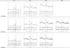 |
Fig. 4. Composite of spectral types along MS, ordered from A1 to A4. Color scheme same as in Fig. 3. |
| In the text | |
|
Fig. 5. CD Hβ centroid shifts (km s−1) for different E1 classes and for different line height. From top to bottom: x = 1/4, x = 1/2, x = 9/10. Bottom: equivalent width (Å) distribution. Blue refers to the RD class, green to the RI one, red to the RL one and black to the RL FRII class. |
| In the text | |
|
Fig. 6. CD [O III] centroid shifts (km/s) for different E1 classes and for different line height. From top to bottom: x = 1/4, x = 1/2, x = 9/10. Bottom: equivalent width (Å) distribution. Blue refers to the RD class, green to the RI one and red to the RL one. |
| In the text | |
|
Fig. 7. Equivalent width of [O III]λ5007 as function of spectral types for CD RD, RI, RL sources. Upper panel: refers to the base, semi-broad component, the bottom one to the narrower core of the [O III]λ5007 line. |
| In the text | |
|
Fig. 8. CD B1 Hβ (top) and CD A2 [O III] profiles (bottom) for different radio power classes. Blue refers to the RD class, green to the RI one and red to the RL one. |
| In the text | |
|
Fig. 9. FIR luminosity vs. radio power. The shaded areas trace the occupation zone of star-forming galaxies (gray) and RQ quasars (pink) following Bonzini et al. (2015). Color codes are: red (RL), green (RI), blue (RD). Left: sources identified on the basis of spectral types; xA: circled symbols; A2: circles; A1: pentagons; B1: squares; B2: rhomboids; not defined: open symbols. Right: sources identified on the basis of samples. Circles: this work; rhomboids: Marziani & Sulentic 2014, squares: Sani et al. 2010 + Marziani et al. 2003. |
| In the text | |
|
Fig. 10. Distribution of radio power Pν in units of W for RI (top) and RL (bottom), for different spectral types along MS. Top panels: distributions for the union of B1++ and B1+ (red), B1 (orange) spectral types, the bottom ones for A1 (gray), pale blue (A2), and xA (blue). The vertical dot-dashed lines mark the medians of the Pop. B (red and orange), A2 (pale blue) and xA (blue) distributions. |
| In the text | |
|
Fig. 11. Behavior of radio power Pν in units of W as function of Kellermann’s parameter |
| In the text | |
|
Fig. 12. Behavior of log |
| In the text | |
|
Fig. 13. Top: core-to-lobe radio flux density ratio vs. FWHM(Hβ), adapted from Wills & Browne (1986). Colored dots represent sources of our sample: red dots represent A1 RL FRII sources, yellow dots B1 RL FRII, green B1+ RL FRII and blue ones B1++ RL FRII. Black dots are the original data from Wills & Browne (1986). The magenta line represents the change of R with FWHM(β), predicted by the Orr & Browne (1982) beaming model with RT = 0.024 and γ = 5. Bottom: FWHM(β) vs. inclination, derived from Rc through Eq. (16). |
| In the text | |
|
Fig. 14. Comparison between broad + very broad and double broad Hβ fitting models. From left to right, top to bottom: CD-RD-B1+, CD-RI-B1+, CD-RL-B1+ and FRII-RL-B1++. For each pair the left plot represents the broad + very broad fitting BC+VBC model and the right plot represents the double broad component model BC+BD. Color scheme same as in Fig. 3. |
| In the text | |
|
Fig. A.1. Radio maps at 1.4 GHz for FRII sample from FIRST catalog with size of field 4.5′×4.5′ and Maximum Intensity for Scaling equals to 10 mJy. The images follow the SDSS ID order of Table A.2 from left to right and from top to bottom. |
| In the text | |
|
Fig. A.1. continued. |
| In the text | |
Current usage metrics show cumulative count of Article Views (full-text article views including HTML views, PDF and ePub downloads, according to the available data) and Abstracts Views on Vision4Press platform.
Data correspond to usage on the plateform after 2015. The current usage metrics is available 48-96 hours after online publication and is updated daily on week days.
Initial download of the metrics may take a while.