| Issue |
A&A
Volume 627, July 2019
|
|
|---|---|---|
| Article Number | A47 | |
| Number of page(s) | 18 | |
| Section | The Sun | |
| DOI | https://doi.org/10.1051/0004-6361/201935182 | |
| Published online | 02 July 2019 | |
Formation and morphology of anomalous solar circular polarization
1
Instituto de Astrofisica de Canarias, 38205 La Laguna, Tenerife, Spain
e-mail: This email address is being protected from spambots. You need JavaScript enabled to view it.
2
Universidad de La Laguna, Dpto. Astrofisica, 38206 La Laguna, Tenerife, Spain
3
Istituto Ricerche Solari Locarno, 6600 Locarno, Switzerland
Received:
31
January
2019
Accepted:
28
May
2019
Abstract
Context. The morphology of spectral line polarization is the most valuable observable to investigate the magnetic and dynamic solar atmosphere. However, in order to develop solar diagnosis, it is fundamental to understand the different kinds of anomalous solar signals that are routinely found in linear and circular polarization (LP,CP).
Aims. We aim to explain and characterize the morphology of solar CP signals considering nonlocal thermodynamical equilibrium (NLTE) effects.
Methods. An analytical two-layer model of the polarized radiative transfer equation is developed and used to solve the NLTE problem with atomic polarization in a semi-parametric way. The potential of the model for reproducing anomalous CP is shown with detailed calculations and examples. A new approach based on the zeroes of polarization signals is developed to explain their morphology.
Results. We have obtained a comprehensive model that insightfully describes the formation of solar polarization with certain precision without sacrificing key physical ingredients or resorting to complex atmospheric models. The essential physical behavior of dichroism and atomic orientation has been described, introducing the concepts of dichroic inversion, neutral and reinforcing medium, critical intensity spectrum, and critical source function. We show that the zero-crossings of the CP spectrum are useful to classify its morphology and understand its formation. This led to identification and explanation of the morphology of the seven most characteristic CP signals that a single (depth-resolved) scattering layer can produce. We find that a minimal number of two magnetic layers along the line of sight is required to fully explain anomalous solar CP signals and that the morphology and polarity of Stokes V depends on magnetic, radiative, and atomic “polarities”. Some implications of these results are presented through a preliminary modeling of anomalous CP signals in the Fe I 1564.8 nm and Na I D lines.
Key words: polarization / radiative transfer / scattering / stars: magnetic field / magnetic fields / Sun: atmosphere
© ESO 2019
1. Introduction
The normal antisymmetric spectrum of circular polarization in solar spectral lines is due to magnetic fields modifying the optical properties of the solar plasma through the Zeeman effect. The frequent variations of antisymmetric signals into asymmetric ones have been well measured and studied. They are typically reproduced by a combination of line-of-sight (LOS) velocity and magnetic field gradients (see e.g., Illing et al. 1975; Sanchez Almeida et al. 1988; Grossmann-Doerth et al. 1989; Solanki 1989; Rueedi et al. 1992; López Ariste 2002).
On the other hand, there is increasing observational evidence showing anomalous circular polarization signals that are far from having two antisymmetric lobes. Such nonstandard profiles can have several shapes: only one lobe (Sánchez Almeida et al. 1996; Sigwarth et al. 1999; Grossmann-Doerth et al. 2000; Sainz Dalda et al. 2012); two prominent lobes of the same sign (hereafter double-peak profiles, see e.g., Grossmann-Doerth et al. 2000; Sigwarth 2001; López Ariste et al. 2009); three (or four) lobes of alternate signs, which would be called type III (or IV) following Sánchez Almeida et al. (1996) classification, or mixed-polarity types following Sigwarth (2001); or even three lobes with nonalternate signs (Sánchez Almeida et al. 2008; Kiess et al. 2018).
Some of the abnormal Stokes V profiles may be emulated by a multi-component model atmosphere combining quasi-ordinary Stokes V profiles with different amplitudes and spectral shifts, while others have symmetry properties challenging such approach. In any case, one has to consider that almost any polarization profile can be explained by more than one solar atmospheric configuration (spectral ambiguity). Hence, mimicking profiles cannot necessarily be considered as proof of a right modeling. As highlighted in Carlin & Bianda (2017), the spectral ambiguity is a problem when investigating scattering polarization signals because they can be affected by many factors (particularly by atomic polarization, Hanle effect, and chromospheric velocity gradients). If definitive proof of accurate modeling is to be obtained, we need to define discrimination techniques that allow us to clarify, and if possible disentangle, the physical mechanisms in action (Carlin & Asensio Ramos 2015). A posteriori, such constraints could be explicitly introduced in inversion codes to make them immune to spectral ambiguities.
In this regard, one possibility is to study anomalous circular polarization (CP) signals to bypass the complex angular behavior of radiation field anisotropy modifying linear polarization (LP), to complement the information in LP, and to avoid ambiguities. With this idea in mind, we are analyzing, in a separate publication, quiet-sun observations of Stokes V signals taken with the ZIMPOL spectropolarimeter (Ramelli et al. 2010) at GREGOR (Volkmer et al. 2007) in chromospheric spectral lines forming in nonlocal thermodynamical equilibrium (NLTE). We find that they exhibit continuous spatial transformations between near-ubiquitous “Q-like” profiles (three lobes with alternate signs) and double-peak profiles. In that process, anomalous LP signals and chromospheric velocity gradients were identified and need to be explained.
Grossmann-Doerth et al. (2000) and Steiner (2000) studied anomalous Stokes V signals in LTE considering a model of a static magnetic canopy above a nonmagnetic moving layer and emphasizing the presence of their abrupt interface, the magnetopause. This canopy model seeks to have a nonmagnetic moving layer spatially separated from a magnetic layer (Grossmann-Doerth et al. 1989), thus assuring the presence of simultaneous gradients of magnetic and velocity fields along the LOS. The need for this combination to explain the observed Stokes V asymmetries and net circular polarization (NCP) was proposed by Illing et al. (1975) and supported by the work of Sánchez Almeida et al. (1989) under the assumptions of relatively small velocity gradients. However, López Ariste (2002) showed that in a general case with arbitrary velocity gradient its role in generating NCP is key and more fundamental than that of the magnetic field. The association between velocity gradients and the formation of solar CP has been well studied in different physical conditions by several authors (e.g., Martinez Pillet et al. 1994; del Toro Iniesta et al. 2001; Borrero et al. 2010).
Two limitations of the studies cited above is that they try to explain the formation of Stokes V profiles assuming LTE and without considering the role of atomic polarization. This is not suitable for our purposes because spectral lines with anomalous polarization profiles may form in NLTE, typically in the upper photosphere or above (e.g., the Sodium D lines). The action of an anisotropic and/or spectrally asymmetric radiation field in the atomic system (i.e., the generation of atomic polarization) requires in these cases a NLTE solution to the statistical equilibrium equations (SEE). Though NLTE effects may be ruled out for spectral lines forming in volumes that are sufficiently dense so as to be collisionally depolarized, the boundary between the two regimes is unclear, strongly line-dependent, and probably also spatio-temporally dependent. Assuming LTE leads to a second inconsistency: previous works disregard atomic orientation while assuming a radiation field modified by velocity gradients (i.e., with NCP). This has the contradictory effect of inducing atomic orientation, because the Doppler-induced spectral imbalance of intensity modulates the atomic density matrix by means of the radiation field tensor in the SEE (see Eq. (7) in Bommier 1997). Hence, if significant velocity gradients are invoked to explain the circular polarization, the role of atomic orientation should also be investigated.
In the present paper our goal has been to develop a suitable model accounting for any observed circular polarization profile without neglecting the physics of NLTE and atomic polarization. In Sect. 2, we introduce the minimal arguments and physical ingredients to explain Stokes V signals with atomic orientation. In Sect. 3, we present a simple radiative transfer model and propose a first spectral mechanism able to produce double-peak and Q-like V profiles in nonmagnetic atmospheres. In Sect. 4, we use these latter concepts to study with detailed calculations a second spectral mechanism that explains anomalous Stokes V signals with Zeeman splitting. Sections 5 and 6 demonstrate the ability and convenience of our theoretical description in explaining any CP signal.
2. Preliminars
2.1. Atomic orientation
In a statistical collectivity of scattering atoms, an atomic level J ≠ 0 (or F ≠ 0 for atoms with nuclear spin) is oriented when there is an imbalance of electronic population between Zeeman sublevels whose magnetic quantum numbers M have opposite signs. This is expressed as ρ−M − M(J)≠ρMM(J) in the standard representation of the atomic density matrix. In the multipolar representation, atomic orientation is instead quantified by tensor components of the atomic density matrix  with rank K = 1 and Q = 0 (see Sect. 3.6 of Landi Degl’Innocenti & Landolfi 2004, for details). The SEE indicate that atomic orientation can be created by an oriented radiation field, that is, radiation with net angular momentum, characterized by a multipolar tensor component
  . For clarity, the generation of atomic orientation is treated in a separated paper, while here the amount of radiation field orientation is conveniently parameterized by
  , where the mean values of the radiation field tensor are1:
 (1a)
(1a)
 (1b)
(1b)
These equations show that orientation is induced by spectral asymmetries in intensity and Stokes V. This explains why NCP is one of the proxies to radiation field orientation. NCP can be defined as2:
 (3)
(3)
or simply as the numerator when comparing two V profiles whose total number of intensity photons are similar.
2.2. Expected vs. observed weak-field V/I signals
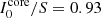
Double-peak profiles and Q-like profiles are the paradigm for nonstandard CP because, having the possibility of being symmetric, they strongly differ from the antisymmetric Zeeman signals. Hence, when trying to explain the anomalies, one of the first logical doubts is whether the Zeeman effect is relevant. We know that in weak fields the transversal Zeeman effect is of second order and as a consequence the typical three-lobe LP signatures do not normally appear for fields below 100 G. Indeed, in Na I D2 the lateral lobes in Stokes Q (formed by the Zeeman σ components) are comparable to the central π component only for field strengths above 200 G (Fig. 1, upper central panel). On the contrary, the longitudinal Zeeman effect is already measurable for strengths as small as 10 Gauss (Fig. 1, right upper panel). Hence, the Zeeman effect seems necessary to explain double-peak patterns. However, the conservation of angular momentum requires any pair of σ+, σ− components to always have opposite sign. Therefore, something else than just the Zeeman effect is required to produce such anomalous profiles.
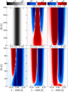 |
Fig. 1. Behavior of V/Ic when varying the magnetic strength and the size and sign of the radiation field orientation without gradients along the LOS. All polarization panels share the same color scale saturated to 1%. Stokes Q and I are plotted as a reference. The example corresponds to the Na I D2 line modeled in a multilevel atom with hyperfine structure for a magnetic vector inclined 70° from the LOS. |
On the other hand, the NCP of nonantisymmetric V signals can induce orientation, as mentioned above. Indeed, the mere existence of Stokes V signals with only one sign should imply a significant increment of the atomic orientation because they can carry an order of magnitude more NCP than normal signals. To see this, one can calculate the integral under the curve of a double-peak CP profile and compare it with the same integral for a realistic standard antisymmetric profile of the same amplitude. As shown by Fig. 2, the former integral is 21 times larger than the latter, simply because the amount of signal that was subtracted in the integral of the antisymmetric profile is now contributing positively. In the particular case of the observation in Fig. 2, the NCP (which furthermore accounts for differences in intensity and polarization amplitudes) is 22 times larger in the double-peak profile. This supports the idea that the existence of atomic orientation in the scatterers is an ingredient to be considered in the formation of anomalous V profiles.
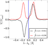 |
Fig. 2. Observed double-peak Stokes V profile (red) vs. standard V profile (black) normalized to their maximum amplitudes (0.2% and 0.1%, respectively) in the Na I D1 line. The profiles were measured at the THEMIS solar telescope. See similar profiles (taken in same campaign as ours) in Fig. 5 of López Ariste et al. (2009). We also found them in Fig. 3 of Bommier & Molodij (2002). |
However, atomic orientation cannot act as a spectral mechanism inverting only one of the peaks of Stokes V unless such an effect is replicated in the optical coefficients of the radiative transfer equation (RTE). This is not possible because the increment of atomic orientation always enhances the contribution of one set of Zeeman sigma components (e.g., the σ+) at the expense of the other. For weak fields, the spectral result is the fusion of both peaks in a single asymmetric peak3. This is illustrated by a comparison between the right upper panel and the lower panels of Fig. 1. Here we have induced atomic orientation in the atoms of a slab model by pumping it with an oriented radiation field. Thus, the ordinary signals are such that, when the Zeeman splitting tends to zero, the sigma components overlap in frequency, either canceling each other in the absence of orientation (see upper right panel of Fig. 1 for B = 0), or resulting in a single (though irregular/asymmetric) lobe whose absolute amplitude is proportional to the amount of orientation (see lower panels of Fig. 1 for B ∈ [0, 10] G). The difference between the calculations in the left and central lower panels is the amount of orientation: the comparison shows that larger orientation produces visible morphological effects persisting in larger field strengths.
In summary, the larger the magnetic field, the larger the Zeeman splitting, and the less effective the cancelation of sigma components; consequently, more atomic orientation is required to induce the same level of asymmetry in the corresponding Stokes V profile. The other side of this sort of “law of scalability” or self-similarity involves the causality existing between the increment of the velocity gradients (or Doppler shifts) and the amount of orientation that they induce: the larger the former, the greater the latter. Thus, the standard expectation is that orientation wins the morphological battle in layers where macroscopic motions are large, while magnetic fields and depolarizing collisions are weak (e.g., in the chromosphere). At the end of the paper, the role of atomic orientation in intermediate and strong fields is reconsidered in light of our results.
For now, we only conclude that despite the fact that orientation effectively modifies the spectral profile and can induce asymmetries in relation to the velocity gradient, it alone cannot invert the sign of only one peak of Stokes V. Hence, apart from Zeeman splitting and atomic orientation, we still need a third physical ingredient, a spectral mechanism. In the following we study two physical setups able to emulate the observed CP signals. The spectral mechanism of the first one is dichroism induced by atomic orientation. The second one also requires dichroism, but this time combined with uneven excitation of the Zeeman components and, though it can be mimicked without atomic polarization, the latter modifies the signal significantly.
3. Radiative transfer model
We start posing the RTE for the Stokes vector I = (I, Q, U, V)T along a ray Ω as a function of the optical depth τν:
 (4)
(4)
where all the quantities depend on τν and frequency ν, being dτν = −ηIds with s the geometrical distance along the ray. The emissivity vector ϵ = (ϵI, ϵQ, ϵU, ϵV)T quantifies the total emission of intensity and polarization in each plasma element, while the propagation matrix is
with ρ being the anomalous dispersion terms, ηI the total absorption (line plus continuum), and ηQ, U, V the dichroism coefficients.
A detailed explanation of the anomalous Stokes V signal can be achieved ignoring the negligible contributions of stimulated emission and second-order terms (of the kind ηiIk and ρiIk when both i, k ≠ 0 ) in the RTE. This leads to
 (5a)
(5a)
 (5b)
(5b)
where S = ϵI/ηI is the total intensity source function. To solve the equations, we consider an arbitrary portion of atmosphere with geometrical size Δs and finite optical thickness Tν = Δs ⋅ ηI (the frequency subindex indicates that each wavelength of the radiation perceives a different opacity). The solutions to the RTE are then
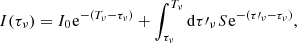 (6a)
(6a)
![Mathematical equation: $$ V({\tau _\nu }) = {V_0}{\mkern 1mu} {{\rm{e}}^{ - ({T_\nu } - {\tau _\nu })}} + \int_{{\tau _\nu }}^{{T_\nu }} {\rm{d}} \tau {\prime _\nu }\left[ {\frac{{{_V} - {\eta _V}I(\tau {\prime _\nu })}}{{{\eta _I}}}} \right]{{\rm{e}}^{ - (\tau {\prime _\nu } - {\tau _\nu })}}, $$](/articles/aa/full_html/2019/07/aa35182-19/aa35182-19-eq12.gif) (6b)
(6b)
with (I0, V0) being the boundary illumination entering the atmosphere4 along the LOS. The outgoing radiation traveling towards the observer is then
 (7a)
(7a)
![Mathematical equation: $$ V(0) = {V_0}{\mkern 1mu} {{\rm{e}}^{ - {T_\nu }}} + \int_0^{{T_\nu }} {\rm{d}} \tau {\prime _\nu }\left[ {\frac{{{_V} - {\eta _V}I(\tau {\prime _\nu })}}{{{\eta _I}}}} \right]{{\rm{e}}^{ - \tau {\prime _\nu }}}. $$](/articles/aa/full_html/2019/07/aa35182-19/aa35182-19-eq14.gif) (7b)
(7b)
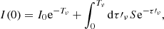
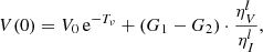
Introducing Eq. (6a) into Eq. (7b) and assuming that all the quantities but the source function are constant with position inside the slab we obtain
 (8)
(8)
In general, the quantities I0 = I0(ν) and S = S(ν, τν) have spectral structure. For consistency with the previous step we assume that S is constant with depth. Working with the total optical coefficients  and
and  , integrating, and reorganizing, we arrive at the useful expression,
 (9)
(9)
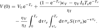
where
 (10a)
(10a)
 (10b)
(10b)
and  . Finally, the emergent fractional polarization is
 (11)
(11)
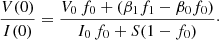
This model is also valid for LP substituting the letter V by Q or U in the corresponding quantities. Equation (9) has three contributions: a first one, due to the boundary illumination, becomes quickly negligible for Tν ≳ 2; a second one depends on the relation between SV and S (contained in β1); and the last one depends on the relation between I0 and S (contained in β0). Each term includes a transfer function f depending on Tν. The dependence on magnetic field and atomic orientation is contained in the optical coefficients.
4. Spectral mechanism without Zeeman splitting
We now consider an academic situation in which: (a) the magnetic field is zero, which implies optical coefficients with a single lobe, as explained in Sect. 2; (b) a given amount of atomic orientation has been induced by pumping with a radiation field  and (c) the illumination along the LOS is spectrally flat. In this situation Eq. (9) can emulate all the spectral features of double-peak and Q-like Stokes V signals, namely: the double peak structure, the asymmetry and distance between the peaks, and the depth of the central dip. Figure 3 illustrates how such a spectral mechanism works. The factor f0 is equal to one in the wings and approaches zero in the core, such that when multiplied by
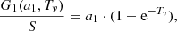
  can produce a double-peak profile. Subtracting the result from the term depending on f1 amplifies the contrast (and the eventual asymmetry) between the peaks and produces Stokes V. The term f0 alone only generates two peaks when the maximum total opacity of the atmosphere is above one, as shown in the left panel of Fig. 4. On the contrary, the factor f1 alone can only have one peak (see left panel of Fig. 4) and its role is to increase Stokes V in the line center, thus modulating the central dip and the visibility (contrast) of the double peaks. What we are describing here is nothing but a balance or competition between emissivity (included in the factor β1f1) and dichroism (dominating the factor β0f0). The signal with two peaks of the same sign is possible because the transfer function f0 shapes the dichroic contribution in its central part, which is observable in Stokes V when emissivity is low enough. Due to this sort of self-absorption in polarization, the explanation of the V peaks in this situation emphasizes the role of dichroism.
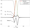 |
Fig. 3. Generation of an asymmetric double-peak profile with B = 0 and atomic orientation (w1 = 5%) following Eq. (9). The quantities represented in the vertical axis are labeled inside the figure but only their shapes are important here. The green curve is normalized to one, and the black curves are multiplied by the same constant, in order to plot everything together. The factors ϵV and ηV were calculated for the Na I D2 line in a multilevel atom with HFS. |
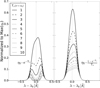 |
Fig. 4. Origin of the double-peak spectrum in Fig. 3 as a function of the optical depth of the slab Tν, following Eq. (9). Left: factor generating a double-peak profile. Right: factor opposing the generation of the peaks. |
In a static unmagnetized media such as the one considered, the asymmetry between the V peaks is due to the optical coefficients. The deviation that these coefficients can have from a Gaussian comes from atomic orientation and from the asymmetric spectral distribution of Zeeman components (due to HFS in case of our archetypal Sodium atom). In the numerical experiment of Fig. 3, only ηV is asymmetric, while ϵV remains practically symmetric. The particular asymmetry of one or other coefficient can change depending on the atomic species, the transition, and the solution to the SEE. Figure 3 shows that the deviation that ηV shows from the symmetric (Gaussian) profile is transformed efficienly into a significant asymmetry in Stokes V during the radiative transfer. This happens at the level of the atomic collectivity, without the need for macroscopic motions.
4.1. The essential behavior of dichroism
The simplicity of our model allows us to study analytically the action of dichroism and its balance with emissivity. In our context, the only ways of having dichroism, that is, a selective absorption of polarization states in an atom, are to have a Zeeman splitting making the absorption selective in wavelength, and/or to have atomic polarization (the only possibility in unmagnetized fluids or in magnetic plasmas when the magnetic field is not longitudinal). In order to decipher the conditions in which the paradigmatic double-peak signals are formed with our first (non-magnetic) spectral mechanism, we reformulate Eq. (9) using quantities normalized to the source function:
 (12)
(12)
where
 (13a)
(13a)
![Mathematical equation: $$ \frac{{{F_2}({\alpha _2},{T_\nu })}}{S} = \frac{{1 - {{\rm{e}}^{ - {T_\nu }}}\left[ {1 + {T_\nu }(1 - {\alpha _2})} \right]}}{{{T_\nu }}}, $$](/articles/aa/full_html/2019/07/aa35182-19/aa35182-19-eq27.gif) (13b)
(13b)
 (14)
(14)
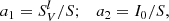
We now simplify these expressions by approximating the optical coefficients using spectrally symmetric Gaussians because there is no Zeeman splitting, which allows us to make the following simplifications5:  and similarly
 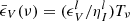 , with the index l indicating line coefficients. This simplification is only used in the following few paragraphs for illustrative and explanatory purposes. The new formulation is then
 (15)
(15)
 (16a)
(16a)
![Mathematical equation: $$ \frac{{{G_2}({a_2},{T_\nu })}}{S} = 1 - {{\rm{e}}^{ - {T_\nu }}}\left[ {1 + {T_\nu }(1 - {a_2})} \right], $$](/articles/aa/full_html/2019/07/aa35182-19/aa35182-19-eq33.gif) (16b)
(16b)
 (17)
(17)
where the dependence of the polarization on frequency and optical depth is now exclusively contained in G1 and G2. The left panel of Fig. 5 shows the variation of the two families of curves F1 (black lines) and F2 (red lines) with optical depth for different α1 (relative Stokes V line source function) and α2 (relative incident intensity), respectively. The right panel shows the same for G1 and G2 with their corresponding parameters a1 and a2. Subtracting these latter functions gives Stokes V up to a constant. Thus, small values of a1 shift down6 the black curves in the right panel of Fig. 5, leaving the emergent polarization dominated by G2(a2, Tν). Indeed, when the G1 curve goes below the bumps of G2, the bumps themselves become the double peaks in the Stokes profile because each frequency of the light corresponds to a different opacity and optical depth. Namely, fixing the maximum optical depth of the slab in Tν and varying the frequency from the core to the wings of the spectral line corresponds to sampling the curves in Fig. 5 toward smaller optical depths. On the contrary, fixing frequency in the emergent profile and starting to accumulate optical depth as we penetrate the slab corresponds to sampling the curves from zero to the maximum optical depth of the slab, where a boundary I0 illuminates.
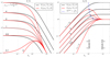 |
Fig. 5. Left: variation of F1/S and F2/S with optical depth for different levels of V source function (α1 = SV/S) and intensity (α2 = I0/S), respectively. Right: same as left panel but for G1/S and G2/S with their corresponding parameters a1 and a2. Limiting values are: F/S(α1, Tν ≥ 10) = α1/Tν, G/S(a1, Tν ≥ 10) = α1 and G/S(a1, 2, Tν ≪ 1) = a1, 2Tν. |
The bumps in G2 are at the same point where the sensitivity to the illumination is maximum, that is, where the depth penetrated into the slab is around Tν = 1. The sensitivity to the illumination quickly saturates around Tν = 10 (clearly, if the slab is too opaque nothing is transferred). The curves also show that the formation region of the polarization is essentially between Tν = 0.1 and 10 at every frequency, as happens with intensity. Since polarized photons are part of the whole intensity, their formation regions are quoted by the same optical depths.
From Eq. (16b) we calculate the optical depth  corresponding to the maximum of the bumps of G2:
 (18)
(18)
which gives the blue curve trending asymptotically to Tν = 1 in the right panel of Fig. 5 as I0/S increases. This simply means that in a real atmosphere the modifications of the polarization profile due to dichroism are maximum around the height of τ = 1 for a given frequency. For an illumination varying with frequency, the same discussion is applied independently to every frequency.
We also note that a significant part of the region where G2/S has negative slope is mapped for optical depths  .
.
The aim of working with G2/S (F2/S) has been to expose the dichroic response and the formation of peaks for relatively strong (weak) illuminations, as illustrated by Fig. 5. In the right panel, the bumps in G2/S disappear when the red curves become monotonic (a2 = I0/S ≤ 1), that is, when the illumination is not able to surpass the emissivity of the slab. In this (and in any) situation G2 is still not zero. Thus, provided that there is also emissivity and enough opacity, G1 and G2 can still develop peaks in the Stokes profile when the illumination drops below a certain limit. The easiest way of seeing this is to identify such low-intensity peaks with the bumps appearing for α2 < 0.5 in F2 (see left panel of Fig. 5).
Figure 6 shows double-peak and Q-like Stokes V signals with lateral peaks formed with low intensity (darkest blue curves) and high intensity (darkest red curves). While the former ones are limited in amplitude, the latter ones increase with the incident intensity.
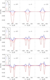 |
Fig. 6. Stokes V normalized to the continuum intensity in the Na ID1 line for B = 0, constant w1, and for different constant boundary illuminations (α2 = I0/S) and positive values of α1 = SV/S. Top (Tν0 = 1): opacity is not enough to create the peaks. Middle (Tν0 = 5): peaks are clearly formed. Bottom: (Tν0 = 10): peaks are fully contrasted and start to saturate. The level of the central dip depends on the Stokes V emissivity. |
Besides, for a constant illumination along frequency, small opacities (≈3) create less contrasted peaks while large opacities (≈10) create a well-defined central dip as a saturation effect (Fig. 6). Such line-core saturation renders the outgoing polarization independent of the illumination and thus the amplitude and sign of the dip is strongly determined by the emissivity, through the parameter α1, as seen in the lower panels of Fig. 6.
In other words, the self-absorption effect producing the central dip in the polarization profile is not increasing with opacity nor I0 once saturation is reached. As a result, the sign and depth of the central dip are only determined by the balance between emissivity and a (saturated) absorption of circular polarization. When opacity increases further, saturation extends to outer wavelengths, where the peaks become more separated and smaller.
A nonmagnetic model such as this first one seems unsuitable for most anomalous solar V signals because it would require a scattering layer with unrealistically high temperatures (to fit the width of the profiles). Yet, the previous explanations have served to characterize the action of dichroism and are useful in the rest of the paper.
4.2. Condition of neutral medium and dichroic inversion
Equation (9) and our previous figures show that in an optically thick atmosphere Stokes V is minimized at frequencies in which the term depending on the emissivity of circular polarization cancels exactly the term controlled by the illumination (F1 = F2). In such a case we say that the medium has become optically neutral for Stokes V because the action of emissivity and dichroism are in a sort of equilibrium. When this happens only at line center in the context previously described (with atomic orientation but without magnetic field) the result is fully contrasted double-peak V signals.
Strictly speaking, Eq. (9) shows that a neutral medium at a given wavelength yields an outgoing polarization that is the one entering the slab but attenuated: V = V0 ⋅ e−Tν. Accordingly, observing a zero crossing in Stokes V does not necessarily mean a neutral medium at that wavelength unless the background does not produce significant V0 along the LOS and/or the formation region is opaque enough to dampen it.
The right panel of Fig. 7 shows the emergent Stokes V with our model for the same slab with neutral medium at line center but changing only the Stokes V0 profile (left panel) at the incoming boundary of the slab. It is illustrative to see that, though V(λ0)≠0 when V0 ≠ 0, the deviation from zero is relatively small at line center (where opacity is the largest in a slab of limited geometrical width), even for strong incoming signals. Instead, the symmetry of the emergent signal can change if the medium becomes thin at other wavelengths. In the example of the figure, we have considered that in the presence of velocity gradients along the LOS and magnetic fields in lower layers, the slab will be illuminated by a shifted and very asymmetric V0, as is the case for those in the left panel of the figure.
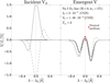 |
Fig. 7. Effect of an asymmetric V0 in a nonmagnetic slab of reduced opacity that is illuminated by a spectrally flat intensity. |
The condition of neutral medium for a Stokes parameter k = Q, U, or V can be written in several ways that relate the parameters of the model. Some insightful relations are obtained for an atmosphere that is not optically thin (Tν ≳ 3). For instance7:
 (19)
(19)
with Sk = ϵk/ηk. Alternatively,
![Mathematical equation: $$ \begin{aligned} \frac{S_k}{S}= \frac{1-f_0[1+T_{\nu }(1-\alpha _2)] }{1-f_0}\cdot \end{aligned} $$](/articles/aa/full_html/2019/07/aa35182-19/aa35182-19-eq39.gif) (20)
(20)
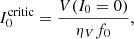
We can also express this as a function of a critical intensity  illuminating the slab along the LOS. For instance, for Stokes V we have
 (21)
(21)
which implies that
 (22)
(22)
Finally, the same condition written in terms of the ratio 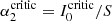 is
is
![Mathematical equation: $$ \begin{aligned} \alpha ^\mathrm{critic}_2= 1+\left[\frac{S_k}{S}-1 \right]\cdot \frac{f_1}{f_0}\cdot \end{aligned} $$](/articles/aa/full_html/2019/07/aa35182-19/aa35182-19-eq44.gif) (23)
(23)
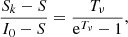
This latter expression provides a useful estimation of the critical value that the I0 has to cross for the sign of the polarization to change at a given frequency (dichroic sign inversion); this inversion depends on the imbalance between emission and absorption for the Stokes parameter considered.
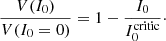
Here we comment on two cases in Eq. (23). The first one is when Sk/S = 1, which gives  : in order to invert the sign of the polarization, I0 has to jump above or to diminish below the value of the intensity source function. A second case is when Sk/S = 0 (no emissivity for Stokes k), which implies
 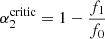 . This value is always negative, so cannot be crossed by a physical I0/S > 0. This simply means that in the absence of emissivity of polarization the dichroic sign inversion is not possible under solar conditions. Hence, there is a minimal emissivity and a minimal critical value
  that guarantees
  in Eq. (23). For Stokes V this occurs when
 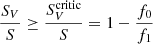 (see Fig. 8). Note that SV < 0 is possible but still subcritical: only SV > 0 allows for a dichroic sign inversion.
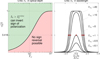 |
Fig. 8. Left: critical values (black line) of the quantity SV/S = (ϵV/ηV)/(ϵI/ηI). If SV/S > (SV/S)critic (green region), then an |

When the LOS optical depth increases at a given wavelength, then  . An SV > S is possible, but our preliminary tests indicate that the larger the
  , the more difficult it is to have an SV above it. In other words, it is more difficult to have ϵV/ηV > ϵI/ηI. Thus, the probabilities of a sign inversion are lower for larger optical depths along the LOS. Paying attention only to Tν ≈ 1, where the sensitivity to the dichroic modulation is maximum for a given frequency ν (remember Fig. 5), the critical value is a more feasible
 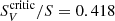 (Fig. 8).
Finally, note that ηV has zeros making SV = ∞. This should not lead to confusion; SV is only a derived quantity that we are using here for convenience and compactness. When  is explicitly inserted into Eq. (12),
  and the poles disappear from the denominator, always yielding finite Stokes parameters. A more detailed study relating
  with the spectrum of the optical coefficients and the atomic properties is presented in a separate publication.
4.3. Condition of reinforcing medium
We define a reinforcing medium as one in which the polarization contribution of dichroism is added constructively to the one of emissivity at a given frequency. From Eq. (9), this interesting situation implies
 (24)
(24)
The arrow follows from the fact that in the first inequality only SV can be negative because S, the denominator, and the transfer functions are always positive8, regardless of the optical depth and I0.
A superficial inspection of the equations of the optical coefficients shows that in general the relative sign of ϵV and ηV depends on the signs of the polarizability coefficients and on the sign and amount of atomic orientation in each level of the atomic transition. While the polarizability coefficients can be tabulated for different atomic transitions (see e.g., the coefficients for HFS in Table 10.7 of Landi Degl’Innocenti & Landolfi 2004), the sign of the orientation in each atomic level depends in general on the geometry of the pumping radiation field (e.g., through  ) and on the detailed solution of the SEE.
Considering for a moment a weak magnetic field along the LOS, and in the particular case of the Na I D1 line optically pumped without radiation field orientation, we find that both ϵV and ηV always have the same sign, frequency by frequency, meaning that no reinforcing medium is possible. This is true even though their signs change together with frequency due to the Zeeman splitting. We then find that the only requirement for having a frequency interval with opposite signs in ϵV and ηV (hence, a reinforcing medium) is a “dephase” between the (Zeeman-induced) zero crossings of both optical coefficients. An analysis of optical coefficients including the physics of scattering polarization shows that in Stokes V the dephase can be simply achieved with atomic orientation, as shown in Fig. 9. Thus, atomic orientation is able to open spectral windows where the polarization amplitude could be reinforced. The width of the window decreases with the magnetic field strength but increases with the atomic orientation. As such windows are around the zeroes of the optical coefficients, the reinforcement of the amplitude by this mechanism seems in general limited.
 |
Fig. 9. In green, region where SV < 0 due the ability of atomic orientation ( |

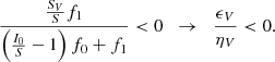
Figure 10 summarizes the concepts of neutral medium, reinforcing medium, and dichroic inversion. When α1 < 0 the medium is reinforcing and the illumination cannot change the sign of the emergent polarization at a given wavelength, which is always the sign given by emissivity. When α1 > 0 the illumination existing at a given optical depth can induce a dichroic sign inversion if α2 crosses the critical value delimited by the (black) lines in the figure. We advance that a Doppler brightening produced by velocity gradients along the LOS can produce first a cancelation of the signal and then enter in a regime of amplitude enhancement, in which larger intensities produce larger signals with an opposite sign to the one in the initial static situation.
 |
Fig. 10. Quantity |

 |
Fig. 11. Scheme of the first version of our model for polarization. |
5. Dichroism with Zeeman splitting
In the following, we investigate the mechanism by which the Stokes V signals are generated in the presence of magnetic fields, NLTE, and atomic polarization. We have extended the model of previous sections to consider Zeeman splitting, a spectral-line profile for the illumination I0, and a relative LOS macroscopic motion between lower layers (those generating I0) and upper layers (main scattering region). Equation (12), or equivalently Eq. (9), still applies and forms the basis of the model but now the optical coefficients must additionally account for magnetic effects such as the Zeeman splitting. In order to describe the radiative transfer for a generic spectral line, the temperature (T), the LOS velocity (υLOS), the magnetic field (B) of the slab, and the minimum of I0 are parameterized through the generalized variables:
 (25a)
(25a)
 (25b)
(25b)
 (25c)
(25c)
 (25d)
(25d)
where ΔλD is the thermal width of the absorption profiles at the scattering layer, ΔλB is the corresponding Zeeman splitting,  is the effective Landé factor associated to the transition, νL[s−1] = 1.3996 × 10⁶ ⋅ BLOS[G] is the Larmor frequency of the longitudinal magnetic field component, and w is the spectral width at half depression of the incident line profile I0 (or at half amplitude if I0 is in emission). The factor α quantifies the relative width among the background intensity profile and the absorption coefficient. We have also defined the relative darkening δ (defined as < 0 when I0 < S), to be used in the following section.
The parameters α, β, and ξ are in units of ΔλD. Expressing ξ in units of w is just a matter of dividing by α. In general, one may also work in units of the total FWHM of the ηI of the scattering layer by multiplying α and ξ by9 3/(5 + 6β), or simply by 3/5 if the magnetic broadening is negligible. The idea is to include as many broadening mechanisms10 as possible in these relative definitions between the layers, but in this paper we simplify by only using variables in Doppler units.
Regarding the velocity, what is important to explain the signals is the velocity gradient between the main and the lower (background) layers. Hence, the analysis is simplified by setting the velocity of the lower layers to that of the laboratory frame (i.e., to zero) and measuring the slab velocity with respect to this latter (velocity is positive when towards the observer). Thus, ξ is a measure of both velocity and velocity gradient. The effect of velocity gradients is two-fold: On one hand, they introduce a Doppler spectral shift between the pumping field and the absorption profiles of the main formation region. Velocity gradients along the LOS thus produce Doppler brightenings at such heights, increasing I0 and bringing the possibility of a dichroic sign reversal. On the other hand, they increase the amount of atomic orientation by affecting the contribution of the radiation field to the rate equations. To consider this latter effect in the following numerical experiments, we have set an ad-hoc fractional radiation field orientation w1 = 5% for both D1 and D2 transitions of Na I. Following the approach in HAZEL (Asensio Ramos et al. 2008), we calculated the rest of the radiation field tensors by using the angular and frequency dependence of the photospheric solar continuum radiation tabulated by Pierce (2000). With the information on the radiation tensor, the atomic density matrix is calculated by solving the SEE in NLTE. However, for calculating the emergent Stokes vector we did not use the average values of Pierce (2000) in the LOS lower-boundary condition of the RTE. Instead, we introduced ad-hoc intensity profiles and thus investigate the dependence of the emergent circular polarization to the LOS illumination. This change significantly increases the diagnostic capability of HAZEL without the need of multi-layer radiative transfer.
5.1. Detailed explanation of the formation of Stokes V anomalies
We can now explain some basic results of our model. Figure 12 shows ad-hoc background intensity profiles (upper panels) with the corresponding emergent intensities (middle panels) and emergent circular polarization (lower panels) calculated in four cases of interest (one per column) for the Na I D1 line. The only parameters of the experiments that change among columns are the LOS Doppler velocity ξ and the radiation field orientation  . To ease the explanation, in this section the background polarization V0 is set to zero.
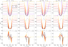 |
Fig. 12. Formation of NLTE circular polarization with atomic polarization and velocity gradients in the Na I D1 line. The figure indirectly explains why the double-peak and Q-like V signals of the solar Na I D lines are more often found near the solar limb (black profiles) than at the disk center (yellow). The calculation is done with μ = 0.1, Tν0 = 4, α = 3.14 (with T = 6.5 kK and microturbulent velocity υmicro = 6.5 km s−1), Ic = 2 × 10⁻⁵ (cgs units), β = 0.01 (B = 154 G with B parallel to LOS vector). Violet lines: critical intensity |

The intensity profiles in the upper panels are symmetric and centered on λ0, with different minimum (i.e., line center) amplitudes I0(λ0)/S but the same spectral width w, chosen to resemble the width of the observed solar profiles of this spectral line (Stenflo et al. 2000, 2001). The violet line here is the critical intensity producing a neutral medium, that is, the threshold marking the dichroic sign inversion of the emergent circular polarization. The only difference between each upper panel is that the critical intensity is no longer spectrally flat when atomic orientation is present in the scattering layer (i.e., when SV departs from S; see Eq. (23) and the following sections for details).
The optical coefficients for absorption and emission (gray lines in middle and lower panels) are plotted with arbitrary amplitudes, simply to have a reference of their spectral shape; they have a total broadening that is smaller than the total width of the background I0. Note that when the total opacity Tν0 of the scattering region along the LOS is above one (optically thick plasma), the width of the intensity spectrum does not correspond to the thermal width. In these numerical experiments, Tν0 = 4, and then opacity saturates the profile enhancing its spectral width beyond the thermal value. This well-known effect is spectrally identical to that shown for SV in right panel of Fig. 8.
In all cases of Fig. 12 the emerging intensity follows other well-known behavior: its value tends to the source function of the slab, thus producing an absorption or an emission for incident intensities above or below S, respectively. In this sense, the four emergent intensities only differ in that when a Doppler shift is considered (second and fourth columns), the optical profiles are shifted with respect to the illumination and consequently the part of the intensity profile that is affected by it is also shifted. Here this effect is referred to as kinetic broadening.
Let us analyze Fig. 12 column by column. The first column corresponds to a situation with no atomic polarization or Doppler shifts. Observing the upper and lower panels of this column, we see that in wavelengths where the absorption profile captures subcritical incident intensities (darkest profiles) the emergent Stokes V develops additional central peaks whose signs are opposite to those in any other wavelength and/or cases in which the incident intensity is above the critical value. Without velocity gradients or atomic orientation, the sign reversal of such central peaks is symmetric around line center, and consequently the emergent CPs remain anti-symmetric. As explained in previous sections, the sign reversal is a result of the competition between dichroism and emission when the source function for Stokes V is positive. When the whole I0 captured by ηV is supercritical (lines with yellowish-warm colors), the V profiles can only have two peaks. The same would happen if in the absorption band the intensity profile were fully below the critical value.
The second column of panels in the figure illustrates the pure effect of a velocity gradient between the lower atmospheric layers and the region of formation of the emergent Stokes V. The relative Doppler shift between I0 and the absorption profile causes the absorbing atoms to capture more light of the line wing (Doppler brightening) and increases the spectral asymmetry of the background intensity between the peaks of ηV. Such spectral asymmetry would be maximized for all the intensity profiles when the Doppler shift is |ΔλD ⋅ 5/3| (i.e., |ξ| = 5/3). In this figure we arrive only to |ξ| = 0.8, and only for the darkest profiles does the Doppler shift approach a crosspoint between the critical intensity and I0 (neutral medium). Thus, intensities ranging from supercritical to subcritical values (only in the blue half of the profiles, where also SV > Scritic) switch that half of V/I from positive to negative values, changing the profile from antisymmetric to a signal with only one sign, thus giving a double-peak profile.
One could say that the red half of the Stokes V spectra in the bottom panel of the second column is dominated by dichroism, while the blue halves of the two cases with the weakest intensities are dominated by emission of circular polarization. However, this could be misleading because it is actually the balance between emission and absorption that is important: if any of the two contributions disappear, the anomalous signals cannot be explained with Zeeman splitting. Thus, as the background (say photospheric) intensity is significantly stronger near disk center than near the limb, the disk center signals can be more often dominated by dichroism, while exhibiting wavelengths dominated by emission near the limb. This can be counter-intuitive, but we remark that the variations of Stokes V at the red lobes in our example are all dominated by dichroism because I0 is always supercritical and opacity is still significant. It is in the anomalous lobe (the blue one) where the dichroic contribution tends to zero when I0 is low.
Subsequently, the rule in this kind of situation is that the sign reversal (with respect to a situation with supercritical I0) happens in the lobe receiving less background intensity during the Doppler shift. Obviously, as an I0 that is completely subcritical produces antisymmetric V profiles of opposite sign to those for an intensity fully above the threshold, the polarity of the magnetic field cannot be unequivocally deduced without knowing the I0 that illuminates the scatterers. While in intensity a dominance of emission is easily identified as an emission line, in the case of nonanomalous Stokes V signals it is more difficult to decipher because the signal stays antisymmetric and only changes its sign. This sort of ambiguity between magnetic field polarity and an unknown level of background intensity can be avoided in double-peak profiles (and other anomalous signals) if the sign of the relative Doppler shift between different layers is known.
The third column of Fig. 12 shows the result of including a positive radiation field orientation in our numerical experiments. The critical intensity now exhibits two separated spectral branches due to the presence of a zero in the absorption coefficient ηV that is not balanced by a zero in ϵV. Thus, at wavelengths where ηV = 0 the critical intensity presents an asymptote and the amplitude of the Stokes V signals becomes independent of I0, which explains why all the Stokes V profiles coincide at that point. There, Stokes V is only due to emissivity, and has a nonzero amplitude (a central bump) if there is atomic orientation in the upper level. This could be used as an observational diagnosis: if we could identify where ηV = 0, we could calibrate and measure the level of the upper-level atomic orientation at that wavelength. We note that the Stokes V profiles represented with a yellowish line in the third column of Fig. 12, with such a particular enhancement of the line core signal and area asymmetry, have always been very common in observations of the solar photosphere (see e.g., Rueedi et al. 1992).
Including a velocity gradient to the calculation with atomic orientation, we obtain the result of the fourth column in Fig. 12. Now the intensity differences between the red and blue sides are again maximized, as in the second column, and a central bump in V/I appears, as in the third column, resulting in a double-peak profile with a central bump of inverted sign and of amplitude comparable with the other peaks, that is, a Q-like profile. These results show that area and amplitude asymmetries in Stokes V can be created by atomic orientation, which thus contributes to explain Q-like Stokes V profiles.
However, a point to note is that with or without atomic orientation, the Q-like profiles that one can synthesize within the framework of Fig. 12 will not exactly match the observations because the distance between external peaks of the synthetic Q-like Stokes V profiles is unrealistically short. Effectively, we have observed (Carlin et al., in prep.) that in chromospheric lines such as the Na I D lines the distance is always larger than that predicted by the weak-field approximation, meaning that the two peaks of the same sign shown in our figure should be significantly more separated, lying at both sides of the intensity line core to match the observations. Figure 12 shows that the velocity gradient increases that distance, but it proportionally increases the width of the corresponding intensity profile as well, and therefore the problem persists. Thus, in order to complete our explanation additional elements are needed.
5.2. Curling the curl: the NLTE source function and the background circular polarization
To complete the explanation of Q-like profiles, and thus assure that we can explain other polarization signals with our model, we have to include two additional facts. Let us start by considering a chromospheric line observed near the disk center and forming in a magnetic field whose polarity does not change along the LOS. The first fact to examine is the behavior of the NLTE source function which, once decoupled from Planck, can be strongly and systematically decreased with respect to its value in the layers immediately below. On one hand, this decreases the line-core critical intensity triggering a dichroic sign inversion at the scattering layer, as indicated by Eq. (23). On the other hand, it furthermore increases the ratio I0/S via the denominator (and not only via I0 as in Fig. 12). As the source function is modified along the LOS (for instance when it tries to re-couple with the Planck function during the emergence of shock waves), the relation between I0, S, and  changes. With the help of more realistic simulations we are finding that such an interplay is predictable and defines interesting situations. One of them occurs when the intensity line-core goes from supercritical to subcritical (or viceversa) across the whole absorption band, as illustrated by panels 0 and 1 in Fig. 13 using our model. Here we see that radiation is inverting the Stokes V polarity imposed by the magnetic field, hence we talk about a radiative polarity11. This total reversal can happen with and without velocity gradients, depending on the values of ξ, α, S, and Tν.
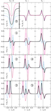 |
Fig. 13. Variation of Stokes V in Na I D1 when changing V0 (see column titles) assuming ξ = 1.3, 0.3, and 0 for bottom, second, and third rows, respectively. Other parameters are Tν0 = 5, B = 100 G, |

The second point to be explained connects the first point with the background V0. While lower layers contribute with a Stokes V component of a given polarity (V0), the upper layers, even when having the same magnetic polarity, can contribute with an opposite radiative polarity (inverted with respect to V0).
When combining these two situations with the partial dichroic inversion induced only in one peak by mild velocity gradients (as explained in Fig. 12), different combinations of signs and amplitudes are possible in the transfer of V0 through the scattering layer, as Fig. 13 demonstrates. In this figure, all V/Ic panels of a given row correspond to identical physical situations in the scattering layer, in particular having the same magnetic field orientation and with a source function that allows total static dichroic inversions when I0 changes as illustrated. However, they differ in V0 by columns: when the longitudinal magnetic field vectors in the foreground and background layers are either parallel or antiparallel, one obtains the profiles in the right-most or middle columns, respectively. When there is only one magnetic layer (V0 = 0, first column), the lateral peaks of Stokes V have both incorrect locations and spectral separations in relation to the intensity profile and to what is observed in the sun. On the contrary, when the background magnetic field is included, the separation between the peaks increases with the velocity gradient, enclosing the intensity core beyond the maximum of its derivative with wavelength (weak-field approx.), as required. Compare for instance black profiles 2 and 4 for small velocity gradient, or 3 and 5 for relatively large velocity gradient in Fig. 13. Thus, combinations of magnetic polarities with velocity gradients develop anomalous CP with distinctive morphologies. Note the triple-peak profile (three peaks of the same sign) in panel 5: it cannot be reproduced with a single magnetic layer.
These results imply that eventual reversals of magnetic polarity that may exist along the LOS (as represented in the middle column of Fig. 13) can play a role in the formation of some of the anomalous CP signals. A more remarkable implication is that multiple unresolved components are not needed to explain the anomalies. This is however a very common approach in the literature. The point is that there is another dimension where resolution matters, and this is the depth along the LOS. Paradoxically, we have deduced the consequences of this fact by reducing the resolution of the radiative transfer along the LOS to a minimal number of two layers.
As an unavoidable consequence of NLTE, the LOS resolution is linked with the variations of magnetic polarity by means of the geometrical extension of the formation region: the more expanded, the more variations (magnetic and dynamical) can it contain, and the more LOS resolution is needed. As pointed out in Carlin & Bianda (2016), an expanded formation region can cover heights with significantly different magnetic field orientations, which in those simulations produced anomalous Q and U signals with different asymmetric spectral profiles in the same pixel.
5.3. Example of application: modeling anomalous polarization in Fe I in 1.5 μm at solar intergranules
Observing quiet-sun intergranular lanes, Kiess et al. (2018) found near-ubiquituous three-lobe Stokes V signals in the 1564.8 nm Fe I line. Carrying out detailed modeling and inversions, these authors concluded that two magnetic field components with very different strengths (9 G and 1147 G) coexisting in the same pixel are required to explain the signals. We synthesized two profiles of their dataset with our model assuming that the signals are instead spatiotemporally resolved. Following a two-level atom approach our preliminary results indicate that the whole Stokes vector can be approximately reproduced by two different scenarios: (1) with a single magnetic layer (V0 = 0) the modeling in Fig. 14 (read caption) is obtained if 3% radiation field orientation is allowed; and (2) with two consecutive magnetic layers along the LOS and without atomic orientation, three-peak profiles can be reproduced as done for Sodium D1 in the bottom-right panel in Fig. 13.
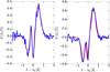 |
Fig. 14. Blue profiles: observations of the Fe I 15648.52 Å (air wavelength) line in the quiet sun (courtesy of Dr. J.M. Borrero; see Kiess et al. 2018). Red profiles: NLTE synthesis obtained with our model assuming a two-level atom for the transition |


Due to the particularities of the Fe I line, more work is required to understand the curious implications of these physical scenarios, and which of the two corresponds to the observation. In addition, we need to reduce the differences with the observation (up to 5% of the continuum intensity) in the wings of the synthetic intensity profile (note that the signals are “inverted” manually, without automatic error minimization). Despite this, we think that the preliminar results support our model as a good starting point for explaining the signals without assuming spatiotemporally unresolved components.
6. Zeroes-based morphology of Stokes V in a single magnetic layer
In this section we use our model to develop a way of understanding the polarization by means of its spectral zeroes. A meaningful approach must start by the case of maximum resolution (in space, time, and in LOS depth), which implies considering that the whole formation region can be represented by a depth-resolved (i.e., single) magnetic layer (V0 = 0). Future developments could then model the spatio-temporal structure of the scattering object (a solar structure, a solar region, or a whole star) to obtain its polarization fingerprint as a combination of the basic pieces explained here. We focus on the most common case of an absorption spectral line in which the effective Zeeman splitting is smaller than the width of the optical coefficients, such that the Zeeman components are not fully resolved. From here, the cases of emission line and very strong field could easily follow.
Unless the contrary is specified, the calculations in this section correspond to solutions of the SEE in the reference atomic system of the Na I D lines. In general, every atomic system has a different efficiency converting radiation field orientation into atomic orientation, and that is why the SEE has to be solved for every line of interest. In this sense, our approach in this section is equivalent to a sophisticated parametrization of the atomic orientation through RF orientation, by means of a reference atomic system that transform one into the other. This approach still allows to extract general conclusions about the polarization signals of any spectral line because its morphology is ultimately due to the radiative transfer part of the problem. Thus, one can first understand the connection between the Stokes signals and the radiative transfer quantities (generalized variables), and then investigate separately the atomic particularities able to produce (or not) those quantities.
6.1. The critical intensity spectrum and the seven representatives of solar circular polarization
The left panel of Fig. 15 shows that atomic orientation (w1) produces a spectrum of critical intensity with two roughly antisymmetric spectral branches: a left and right one. If orientation increases, the critical spectrum bends itself around attractor points at xλ = (λ − λ0 − λD)/ΔλD ≈ ±2. On the contrary, if w1 → 0 the two branches join at right angles where I = S and xλ = 0. The vertical line at xλ = 0 represents a jump (a discontinuity) between 1 and ∞ at the blue spectral side, and between −∞ and 1 at the red side, and must be considered for counting the crossings of Stokes V through zero. Some deviations from this general pattern can be further studied by varying the opacities.
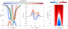 |
Fig. 15. Examples of critical intensity in Na I D1. Left panel: three background intensities (green lines) and their corresponding emergent intensities (black lines) on top of the critical intensity spectra computed for different values of atomic orientation (see discrete color bar) and normalized to Sline = min(S). The gray lines are references corresponding to |


The spectra of critical intensities allow a better understanding of the morphology of polarization signals because the number of times that the illuminating intensity I0 crosses a given critical intensity curve determines the number of zeroes and peaks that Stokes V has, hence its shape. There being M total wavelengths where  , there are N crosses in the wavelength span of the absorption coefficient (“inner” zeroes) corresponding with N visible zeros and N + 1 peaks in Stokes V, with the other M − N zeros now being invisible (“outer” zeros). Sometimes the intensity at a given wavelength does not cross the critical value, but approaches it enough to cancel the V signal significantly. Thus, we shall then say that, among the N inner zeros, some of them can be considered as zeros by proximity, not by crossing.
This simple analysis allows one to quickly classify and understand any polarization signal. Figure 16 and Table 1 show this for the seven circular polarization signals that the author considers the most representative, based on the solar observations cited in the second paragraph of the introduction and on their theoretical interest for solar diagnosis.
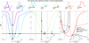 |
Fig. 16. Representative solar Stokes V signals (upper panel) explained by associating their zeros (see legend) with intersections between background (colors) and critical (black) intensities. Vertical dotted lines limit the relevant absorption region (|xλ| < 1). The medium is weakly magnetized (β = 0.05), and optically thick (Tν0 = 3) for all cases, but Tν0 = 1.5 for the three-lobe profile. The values of continuum-to-line opacity (rc = 0.01) and atomic orientation ( |


Morphological classification.
The obtention of Fig. 16 is direct once it is realized that every kind of Stokes V signal forms in specific bins of Doppler velocity (gradient) and I0. The bins in velocity are centered on particular values of ξ that shifts the characteristic points of the absorption profile12 of I0 to the characteristic points of ηV (xλ = 0 and xλ ≈ 1/2), thus giving a total of 20 values of ξ. Studying all of them we could explore the relative variations of amplitude between the peaks of the signal, but the morphological essence (number of peaks and zeroes) is only determined by the points a and a′ marking the wavelengths of neutral medium. This realization leads us to consider only ξ0 = 0 and three characteristic Doppler shifts (plus their symmetric ones) linking velocity and width: ξ1 = 1 − ℓ/2, ξ2 = ℓ/2, and ξ3 = (1 + ℓ)/2. The distance ℓ = |xa − xa′| = p ⋅ w (with p a given fraction of the I0 width w) is generically plotted in the middle panel of Fig. 16. Below, we explain the profiles in the figure:
-
The standard antisymmetric Stokes V signals (and their near-antisymmetric relatives when atomic orientation and/or an imbalance of illumination exists) result from a single cross in the spectral width of the absorption profile that happens when13I0 > S (δ > 0). Any other signal is considered nonstandard and occurs for δ ≤ 0.
-
Four-lobe StokesVprofiles (i.e., three inner zeroes and four peaks) are formed when the I0 core drops below the source function value of the scattering layer with ℓ ≲ 3/2 and Doppler shift ξ ≲ ξ1. The inner peaks are enhanced with a weaker I0. The inner peaks of similar profiles have been associated with magneto-optical effects in Landi Degl’Innocenti & Landolfi (2004) and also with the relative spectral location and strength of the Zeeman sigma components. But we see here that they are easily produced by a mere background intensity with δ < 0. Hence, we think those previous explanations are incomplete, if not incorrect.
-
A double-peak profile (i.e., only two peaks of whichever relative amplitude and width but with the same sign) is exactly formed with a single inner zero that is furthermore at the center of the absorption profile. As deduced from the lower-left panel of Fig. 16, this requires: (1) a velocity gradient shifting the inner zero a to xa = 0 (i.e., ξ = ξ2 = ℓ/2); and (2) an I0 broadening large enough to shift the zero a′ out of the absorption band (xa′ > 1). Substituting ℓ, these conditions imply ξ/p = 0.5 and a minimum I0 width such that p ⋅ α ≥ 1. These conditions can be written in terms of δ if a ligature p = f(δ, α) is set by specifying an I0 profile. It seems incompatible to have atomic orientation and a perfectly symmetric double-peak profile at the same solar location because orientation moves the inner zero away from xλ = 0 regardless of the shape of I0. However, irradiating double-peak Stokes V signals from a solar location introduces orientation in the atoms of the surroundings. Hence, anomalous signals (especially double peaks) may reveal the presence of atomic orientation around their locations.
-
A Q-like StokesVprofile (three peaks of alternating signs) is created when there is a single inner zero per branch. For this, I0 must be deep enough to intersect the two branches of
 , but also broad and shifted enough to intersect each branch only once in xλ ∈ [ − 1, 1]. This implies ξ2 < ξ < ξ1 with ℓ < 0.5. The Q-like profile in this figure has a central peak that cannot be as large as the others: its amplitude is restricted because without orientation, intensity cannot develop significant excursions between the two zeroes (as it did in the rightmost column of Fig. 15). The case without orientation has been chosen to simplify the Fig. 16.
 -
A single-lobeVprofile is a particular case in which a zero by approximation takes place near xa = xa′ ≈ 1/2 (i.e., δ ≈ 0 in case of w1 = 0) with α ≥ 1, which suppresses one lobe. Atomic orientation alters δ, making suppression difficult. As happened with double-peak profiles, this inverse r elation with orientation is counter-intuitive because single-lobe profiles still imply a significant increment of the irradiation of NCP to the surroundings, where signals affected by atomic orientation should then be expected.
-
Figure 16 indicates that three-lobe StokesV signals produced by a single magnetic layer require one zero by crossing, one zero by approximation, and ξ ≈ 1/2, but now the FWHM of I0 must be narrower than half of the absorption band (α < 1). Despite the fact that the calculations indicate that three-peak profiles can be produced without orientation, the relative amplitudes between the peaks (Fig. 14) seem to require orientation (pending confirmation).
6.2. Stokes V zeroes across the space of parameters: atomic polarity and the laws of proportionality.
By exploring the variations of circular polarization with the parameters of our model, we can point out some symmetry properties and reconsider the role of atomic orientation in weak and strong fields.
In the upper panels of Fig. 17, the spectral variations of Stokes V are plotted for strategically sampled values of α, ξ, w1, and Tν0. When considering the continuous changes necessary to connect the different plots, these figures account for many of the circular polarization signals that an absorption spectral line can produce under solar conditions with β < 0.5.
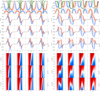 |
Fig. 17. Similar to Fig. 15 but varying α, Tν0, ξ (by columns), and I0 (with α0 = I0/Sline decreasing by rows). Left upper panel: V/Ic for Tν0 = 0.5 and α = 1/3. Right upper panel: as in the left panel but for Tν0 = 3 and α = 1.4. Lower panels: as in upper panels but in two dimensions. |
The lower panels of Fig. 17 highlight in white color the evolution of the zeroes of the circular polarization: anomalous signals appear when there are two or more zeroes in the absorption band. As a side note, we have noted that Stokes V seems to follow a sort of self-similar relationship such that its morphology is preserved when opacity, α, and I0 change together with a nonidentified proportion among them. Let us now focus for a moment on the particular case of a perfectly symmetric double-peak profile, which must have a single inner zero located at xλ = 0 when w1 = 0. If atomic orientation is added, the two branches of critical intensity detach away from their junction at xλ = 0 and the direction of separation depends on the sign of the atomic orientation. Considering now a modification of velocity gradient ξ from the value that produces the double-peak profile, it can be seen (with help of Figs. 15 and 16) that for certain values, the detachment due to orientation leads to two inner zeroes instead of one when  and ξ ≶ 0 (i.e., when velocity gradient and orientation have opposite signs), or no zeroes at all when
  and ξ ≷ 0 (i.e., when they have same sign). This reveals two interesting facts. One is that particular combinations of signs of orientation and velocity gradient are linked to different morphologies in Stokes V. The other is that the ways to explain a given transformation towards a double-peak profile are different depending on the signs of atomic orientation and velocity. In other words, one can always approach a given Stokes V profile from completely different scenarios in the space of parameters. As shown in Fig. 17, this actually holds for any other kind of Stokes V signal, not only for double-peak profiles.
All this is better seen with Fig. 18, when the (redundant) profiles for ξ < 0 are included. Then, the following symmetry property for velocity gradient and radiation field orientation is identified:
 (26)
(26)
 |
Fig. 18. As in Fig. 17 but with |

We note that the effect of velocity gradients of opposite signs is to reverse the red and blue part of the profiles (xλ ↔ −xλ) at the same time as inverting the sign of the signals. Hence, as shown by Fig. 18, all signals can be unequivocally associated to a unique configuration of orientation and velocity gradient (no ambiguity). However, when considering the direction ΩB of the magnetic field:
 (27)
(27)
Now, there is ambiguity (in particular, in the polarity of the magnetic field) when the signals are symmetric around line center. Asymmetric signals can avoid the ambiguity because nothing reverses the profile spectrally without inverting its signs, and because the observer can always distinguish the red and blue halves of a profile. Interestingly, atomic orientation is a source of asymmetry, hence it can contribute to avoiding ambiguity.
6.3. Atomic polarity
Figures 17 and 18 show that there is a third kind of polarity, that introduced by atomic orientation. When the effect of the orientation overcomes that of the magnetic field, most CP profiles adopt a dominant sign corresponding to the sign of orientation. Therefore, at any given wavelength the balance between the three kinds of polarity (magnetic, radiative, and atomic) determines the real polarity of Stokes V. Hence, we realize that in general the combination of these factors causes the concept of polarity for Stokes V to lose its meaning, because the three kinds of sign drivers are in principle uncorrelated and can change along the LOS, producing an arbitrary combination of signs in a given profile. Indeed, that could be the very definition of an anomalous Stokes V signal: one reflecting a combination of polarities (of whichever kind).
To see how difficult the association becomes with a magnetic polarity in a general situation, we can try to define a nonambiguous reference polarity:
Reference polarity (Pr): assuming that a signal is fully resolved in space and time and that the longitudinal magnetic field does not change sign along the LOS, the reference polarity of an antisymmetric Stokes V profile corresponding to a spectral line with geff > 0 and without atomic polarization is defined as positive when the longitudinal magnetic field at the scattering layer points towards the observer (positive magnetic polarity) and I0/S > 1 (positive radiative polarity).
6.4. Laws of proportionality: is atomic orientation relevant when the magnetic field is not weak?
The expected physical situation is that atomic orientation is only important in media with weak magnetic fields, but it is worthwhile investigating some arguments that could challenge this viewpoint. In this paper we start to develop this idea by introducing the following laws of proportionality:
-
Law 1: for producing the same relative morphological change in Stokes V, the more atomic orientation is needed the larger the magnetic field. This was shown in Fig. 1.
-
Law 2: the larger the NCP of a pumping Stokes V radiation field, the more atomic orientation is induced in the pumped scatterers. This is a natural consequence of Eqs. (1) and (3).
-
Law 3: the larger the magnetic fields are in the surroundings of the scatterer, the larger the Stokes V signals are that pump it, simply because the Zeeman components cancel each other less efficiently (they are more separated). As a rule of thumb, Stokes V in hecto-Gauss fields is often an order of magnitude larger than in weak fields.
-
Law 4: if the Stokes V signals pumping the scatterer are anomalous: the larger their amplitudes, the larger the NCP (hence the orientation created). This is especially relevant in double-peak profiles because they only have one sign.
The combination of Laws 3 and 4 with the fact that NCP can be an order of magnitude larger in anomalous signals than in standard signals (see Sect. 2.2), implies that larger magnetic fields may induce proportionally larger atomic orientation. If the proportionality factor is large enough (and this is the key), Law 1 says that similar effects as in weak field should be observed. This argument is reinforced by the results presented in previous sections, which show that the creation of anomalous signals with enhanced NCP does not critically depend on the magnetic field strength, but on the balance between emission and dichroism. Indeed, the possibility of partially changing the Stokes V polarity radiatively implies that, independently of the field strength, similar dichroic sign inversions can also be induced along the other rays of light pumping a scatterer from all directions inside the atmosphere. This seems to be supported by the fact that anomalous CP is observed all over the disk (see observational bibliography in introduction), but also at the limb, as indicated by our measurements with ZIMPOL.
Hence, although caution is advised, we should investigate whether it is possible to find situations where both atomic orientation and hecto-Gauss fields shape the polarization. Two questions arise: Is a three-dimensional optical pumping able to produce visible orientation effects in hecto-Gauss fields? What is the maximum magnetic field strength that allows observation of the signature of orientation? This could be investigated if we confirm our finding about the existence of a stable point where the Stokes V amplitude depends robustly on atomic orientation for any background illumination (Sect. 5.1).
7. Conclusions
By developing a comprehensive two-layer radiative-transfer model, we studied the NLTE generation of anomalous Stokes V signals with magnetic and nonmagnetic dichroism. We considered a first physical scenario able to produce double-peak and Q-like Stokes V signals without longitudinal magnetic field (no Zeeman splitting). This effect consists in the self-absorption of the central part of a polarization profile with only one lobe due to the action of (orientation-dominated) dichroism. Its explanation served to characterize and understand the formation of dichroic polarization from an academic perspective and to introduce useful concepts such as neutral medium, reinforcing medium, critical intensity spectra, and critical source function. Thus, this first version of the model reveals the importance of the balance between polarized emission and dichroism. A remarkable finding was that the signs of the ratio ϵV/ηV and the level of intensity cause dichroism to act on polarization as an amplifying or nullifying mechanism.
Using these concepts we also studied a second scenario based on the uneven pumping of Zeeman components when both magnetic and nonmagnetic dichroism act together. Thus, we identified the basic conditions explaining anomalous Stokes V signals for a generic solar spectral line. The first key is the combination of: (1) dichroism, which allows intensity to modify the polarization; (2) atomic polarization, a form of dichroism that modifies the shape of the optical coefficients and the sensitivity of the atomic system to intensity-driven sign reversals; (3) velocity gradients, which restrict or enhance the action of dichroism at particular wavelengths; and (4) a magnetic field, which naturally allows non-null optical coefficients in cases without atomic polarization and allows to easily explain multi-lobe CP profiles.
The second key to explaining polarization anomalies has to do with the resolution of the physics along the LOS, namely: (1) the particular behavior of the source function for intensity, which can produce a radiative sign inversion of a whole polarization profile; and (2) the need for more than one magnetic component along the LOS to explain all the features of the observed profiles (shape, peak separation, and amplitude). To show this, we used our model to reproduce anomalous double-peak and Q-like profiles such as those observed in Na I D1 and D2, and we presented a preliminary modeling of the observed anomalous CP in the Fe I 1564.85 nm line without the need to assume unresolved magnetic field components. We anticipate that our model allows to reproduce the anomalous CP and intensity measured in the solar context of umbral flashes (Socas-Navarro et al. 2000), again without assuming lack of resolution (paper in prep.).
In general, these results warn against the common assumption of spatially unresolved magnetic components which, justified or not, tends to ignore the origin of the polarization by overlooking the physics of polarized radiative transfer explained here. This emphasizes the need to maximize the spatiotemporal resolution, and the need to verify when a structure is or is not resolved, in order to understand the morphology of polarization and the solar atmosphere.
We also developed an insightful way to explain the polarization morphology using the zeroes of the spectral profiles. The so-called “inner zeroes” are progressively shifted to the line wings and transformed into invisible “outer” zeroes as an increasing velocity gradient between background and scattering layers shifts the minimum background intensity towards wavelengths with insignificant absorption. Thus, the explanation and classification of the seven most representative Stokes V solar profiles followed easily. They were classified as standard (or 11), single-lobe (10 or 01), big-lobe (or 1), double-lobe (or 2), Q-like (or 111), three-lobe (12 or 12), or four-lobe (or 1111). All anomalous signals are produced in conditions of low relative intensity. The morphology of anomalous polarization signals is very sensitive to the line-broadening mechanisms, to dynamics, and to the levels of intensity inside the atmosphere, and for this reason they seem very valuable for testing and improving MHD models. Anomalous CP is easy to find in dynamic simulations and in observations.
We have shown that the polarity of a resolved Stokes V profile is a mixture of magnetic, radiative, and atomic polarities, the anomalous signals occurring when the spectrum is not dominated by only one of them. Regarding atomic orientation, we explained how it modifies Stokes V, emphasizing a law of proportionality between orientation and field strength that is reinforced in the presence of anomalous CP, and that suggests that atomic orientation could play a role in nonweak magnetic fields. Future investigations are needed to confirm whether solar atomic orientation can be effectively measured by identifying in the profile of Stokes V a “robust point” that is stable against changes in background illumination. Finally, our calculations led to the identification of the spectral symmetry relationships relating velocity gradients, atomic orientation, and magnetic field. Asymmetric signals influenced by atomic orientation could be a good candidate for avoiding magnetic field ambiguities. More investigation is necessary in this direction.
Several studies complement this paper. Of particular interest are new observations of anomalous solar circular polarization, the application of our model to LP, and a more detailed study of the optical coefficients modifying the dichroic response of the scatterers.
Here, Ij(j = 0, 1, 2, 3) are the Stokes parameters illuminating the scatterer; 𝒯 are the spherical tensors for polarimetry (Landi Degl’Innocenti 1983); ϕ(ν) are the absorption profiles at frequency ν, and Ω is the direction of each pumping ray at the scattering point.
Another definition is (Landolfi & Landi Degl’Innocenti 1996):
![Mathematical equation: $$ \begin{aligned} \mathrm{{NCP}} = \int \mathrm{d}\lambda \,V(\lambda ) \Bigg / \int \mathrm{d}\lambda \left[ I_{\rm c} -I(\lambda ) \right], \end{aligned} $$](/articles/aa/full_html/2019/07/aa35182-19/aa35182-19-eq91.gif) (2)
(2)
with Ic being the continuum intensity. We do not use this definition because we think that the NCP should be normalized to the total number of photons, not to the depression of the spectral line.
Note that the asymmetry of the optical coefficient depends on the level of orientation, but also on the Zeeman splitting. In an extreme case in which orientation is so strong that depletes one of the sigma components, the result would be a symmetric peak shifting away from line center as the field increases, hence resulting in a completely asymmetric signal in strong field if the axis to measure symmetry is line center.
We model the formation region between vacuum and a maximum optical depth after which an I0 is present.
In this step we are implicitly assuming that the ratio between the continuum and the line absorption for intensity is negligible (strong line), with the only purpose of getting simpler expressions.
Note that G1(a1, Tν > 10) = a1.
The r.h.s. in this equation resembles a Planck function if we associate a “temperature” T = c2/2Kν2 and an opacity Tν = hν/KT = 2hν3/c2.
Stimulated emission does not dominate radiative transfer in stellar atmospheres, hence S ≥ 0.
We relate the Doppler width of a Gaussian profile to its FWHM with FWHM and we add the magnetic broadening with β.
There are seven broadening mechanisms: magnetic, thermal, microturbulent, collisional, opacity saturation, and kinetic (the latter two due to lack of resolution in depth along the LOS). The seventh one is instrumental, due to lack of spatiotemporal resolution.
Stokes V polarity = magnetic polarity × radiative polarity.
The relevant points are: the line center, where I0 is minimum; the crosspoints between I0 and  , where the medium is neutral; and the crosses at the half-width of the profile, where the spectral gradient of I0 is maximum.
Note that regardless of the amount of orientation, the intensities that are above the line source function can cross the critical intensity once.
Acknowledgments
The author thanks L. Belluzzi and M. Bianda for their kind supervision and for useful scientific conversations during the initial stages of this investigation. He is also grateful to J.M. Borrero, for sharing his observations and the details of his investigation, and to N. Bello-González for indirectly helping to orient the results of this paper. This investigation has been partially financed by the Swiss National Science Foundation project 200021_163405 and the Spanish Ministry of Economy and Competitiveness (MINECO) under the Severo Ochoa Program MINECO SEV-2015-0548.
References
- Asensio Ramos, A., Trujillo Bueno, J., & Landi Degl’Innocenti, E. 2008, ApJ, 683, 542 [NASA ADS] [CrossRef] [Google Scholar]
- Bommier, V. 1997, A&A, 328, 726 [NASA ADS] [Google Scholar]
- Bommier, V., & Molodij, G. 2002, A&A, 381, 241 [NASA ADS] [CrossRef] [EDP Sciences] [Google Scholar]
- Borrero, J. M., Martínez-Pillet, V., Schlichenmaier, R., et al. 2010, ApJ, 723, L144 [NASA ADS] [CrossRef] [Google Scholar]
- Carlin, E. S., & Asensio Ramos, A. 2015, ApJ, 801, 16 [NASA ADS] [CrossRef] [Google Scholar]
- Carlin, E. S., & Bianda, M. 2016, ApJ, 831, L5 [NASA ADS] [CrossRef] [Google Scholar]
- Carlin, E. S., & Bianda, M. 2017, ApJ, 843, 64 [NASA ADS] [CrossRef] [Google Scholar]
- del Toro Iniesta, J. C., Bellot Rubio, L. R., & Collados, M. 2001, ApJ, 549, L139 [NASA ADS] [CrossRef] [Google Scholar]
- Grossmann-Doerth, U., Schuessler, M., & Solanki, S. K. 1989, A&A, 221, 338 [NASA ADS] [Google Scholar]
- Grossmann-Doerth, U., Schüssler, M., Sigwarth, M., & Steiner, O. 2000, A&A, 357, 351 [NASA ADS] [Google Scholar]
- Illing, R. M. E., Landman, D. A., & Mickey, D. L. 1975, A&A, 41, 183 [NASA ADS] [Google Scholar]
- Kiess, C., Borrero, J. M., & Schmidt, W. 2018, A&A, 616, A109 [NASA ADS] [CrossRef] [EDP Sciences] [Google Scholar]
- Landi Degl’Innocenti, E. 1983, Sol. Phys., 85, 3 [NASA ADS] [CrossRef] [Google Scholar]
- Landi Degl’Innocenti, E., & Landolfi, M. 2004, Polarization in Spectral Lines (Norwell, USA: Kluwer Academic Publishers) [Google Scholar]
- Landolfi, M., & Landi Degl’Innocenti, E. 1996, Sol. Phys., 164, 191 [NASA ADS] [CrossRef] [Google Scholar]
- López Ariste, A. 2002, ApJ, 564, 379 [NASA ADS] [CrossRef] [Google Scholar]
- López Ariste, A., Asensio Ramos, A., Manso Sainz, R., Derouich, M., & Gelly, B. 2009, A&A, 501, 729 [NASA ADS] [CrossRef] [EDP Sciences] [Google Scholar]
- Martinez Pillet, V., Lites, B. W., Skumanich, A., & Degenhardt, D. 1994, ApJ, 425, L113 [NASA ADS] [CrossRef] [Google Scholar]
- Pierce, K. 2000, in Allen’s Astrophysical Quantities, ed. A. N. Cox (New York: Springer Verlag and AIP Press) [Google Scholar]
- Ramelli, R., Balemi, S., Bianda, M., et al. 2010, Proc. SPIE, 7735, 77351Y [Google Scholar]
- Rueedi, I., Solanki, S. K., Livingston, W., & Stenflo, J. O. 1992, A&A, 263, 323 [NASA ADS] [Google Scholar]
- Sainz Dalda, A., Martínez-Sykora, J., Bellot Rubio, L., & Title, A. 2012, ApJ, 748, 38 [NASA ADS] [CrossRef] [Google Scholar]
- Sanchez Almeida, J., Collados, M., & del Toro Iniesta, J. C. 1988, A&A, 201, L37 [NASA ADS] [Google Scholar]
- Sánchez Almeida, J., Collados, M., & del Toro Iniesta, J. C. 1989, A&A, 222, 311 [NASA ADS] [Google Scholar]
- Sánchez Almeida, J., Landi Degl’Innocenti, E., Martínez Pillet, V., & Lites, B. W. 1996, ApJ, 466, 537 [NASA ADS] [CrossRef] [Google Scholar]
- Sánchez Almeida, J., Viticchie, B., Landi Degl’Innocenti, E., & Berrilli, F. 2008, ApJ, 675, 906 [NASA ADS] [CrossRef] [Google Scholar]
- Sigwarth, M. 2001, ApJ, 563, 1031 [NASA ADS] [CrossRef] [Google Scholar]
- Sigwarth, M., Balasubramaniam, K. S., Knölker, M., & Schmidt, W. 1999, A&A, 349, 941 [NASA ADS] [Google Scholar]
- Socas-Navarro, H., Trujillo Bueno, J., & Ruiz Cobo, B. 2000, ApJ, 544, 1141 [NASA ADS] [CrossRef] [Google Scholar]
- Solanki, S. K. 1989, A&A, 224, 225 [NASA ADS] [Google Scholar]
- Steiner, O. 2000, Sol. Phys., 196, 245 [NASA ADS] [CrossRef] [Google Scholar]
- Stenflo, J. O., Gandorfer, A., & Keller, C. U. 2000, A&A, 355, 781 [NASA ADS] [Google Scholar]
- Stenflo, J. O., Gandorfer, A., Wenzler, T., & Keller, C. U. 2001, A&A, 367, 1033 [NASA ADS] [CrossRef] [EDP Sciences] [Google Scholar]
- Volkmer, R., von der Lühe, O., Kneer, F., et al. 2007, in Modern Solar Facilities - Advanced Solar Science, eds. F. Kneer, K. G. Puschmann, & A. D. Wittmann, 39 [Google Scholar]
All Tables
All Figures
|
Fig. 1. Behavior of V/Ic when varying the magnetic strength and the size and sign of the radiation field orientation without gradients along the LOS. All polarization panels share the same color scale saturated to 1%. Stokes Q and I are plotted as a reference. The example corresponds to the Na I D2 line modeled in a multilevel atom with hyperfine structure for a magnetic vector inclined 70° from the LOS. |
| In the text | |
|
Fig. 2. Observed double-peak Stokes V profile (red) vs. standard V profile (black) normalized to their maximum amplitudes (0.2% and 0.1%, respectively) in the Na I D1 line. The profiles were measured at the THEMIS solar telescope. See similar profiles (taken in same campaign as ours) in Fig. 5 of López Ariste et al. (2009). We also found them in Fig. 3 of Bommier & Molodij (2002). |
| In the text | |
|
Fig. 3. Generation of an asymmetric double-peak profile with B = 0 and atomic orientation (w1 = 5%) following Eq. (9). The quantities represented in the vertical axis are labeled inside the figure but only their shapes are important here. The green curve is normalized to one, and the black curves are multiplied by the same constant, in order to plot everything together. The factors ϵV and ηV were calculated for the Na I D2 line in a multilevel atom with HFS. |
| In the text | |
|
Fig. 4. Origin of the double-peak spectrum in Fig. 3 as a function of the optical depth of the slab Tν, following Eq. (9). Left: factor generating a double-peak profile. Right: factor opposing the generation of the peaks. |
| In the text | |
|
Fig. 5. Left: variation of F1/S and F2/S with optical depth for different levels of V source function (α1 = SV/S) and intensity (α2 = I0/S), respectively. Right: same as left panel but for G1/S and G2/S with their corresponding parameters a1 and a2. Limiting values are: F/S(α1, Tν ≥ 10) = α1/Tν, G/S(a1, Tν ≥ 10) = α1 and G/S(a1, 2, Tν ≪ 1) = a1, 2Tν. |
| In the text | |
|
Fig. 6. Stokes V normalized to the continuum intensity in the Na ID1 line for B = 0, constant w1, and for different constant boundary illuminations (α2 = I0/S) and positive values of α1 = SV/S. Top (Tν0 = 1): opacity is not enough to create the peaks. Middle (Tν0 = 5): peaks are clearly formed. Bottom: (Tν0 = 10): peaks are fully contrasted and start to saturate. The level of the central dip depends on the Stokes V emissivity. |
| In the text | |
|
Fig. 7. Effect of an asymmetric V0 in a nonmagnetic slab of reduced opacity that is illuminated by a spectrally flat intensity. |
| In the text | |
|
Fig. 8. Left: critical values (black line) of the quantity SV/S = (ϵV/ηV)/(ϵI/ηI). If SV/S > (SV/S)critic (green region), then an |
| In the text | |
|
Fig. 9. In green, region where SV < 0 due the ability of atomic orientation ( |
| In the text | |
|
Fig. 10. Quantity |
| In the text | |
|
Fig. 11. Scheme of the first version of our model for polarization. |
| In the text | |
|
Fig. 12. Formation of NLTE circular polarization with atomic polarization and velocity gradients in the Na I D1 line. The figure indirectly explains why the double-peak and Q-like V signals of the solar Na I D lines are more often found near the solar limb (black profiles) than at the disk center (yellow). The calculation is done with μ = 0.1, Tν0 = 4, α = 3.14 (with T = 6.5 kK and microturbulent velocity υmicro = 6.5 km s−1), Ic = 2 × 10⁻⁵ (cgs units), β = 0.01 (B = 154 G with B parallel to LOS vector). Violet lines: critical intensity |
| In the text | |
|
Fig. 13. Variation of Stokes V in Na I D1 when changing V0 (see column titles) assuming ξ = 1.3, 0.3, and 0 for bottom, second, and third rows, respectively. Other parameters are Tν0 = 5, B = 100 G, |
| In the text | |
|
Fig. 14. Blue profiles: observations of the Fe I 15648.52 Å (air wavelength) line in the quiet sun (courtesy of Dr. J.M. Borrero; see Kiess et al. 2018). Red profiles: NLTE synthesis obtained with our model assuming a two-level atom for the transition |
| In the text | |
|
Fig. 15. Examples of critical intensity in Na I D1. Left panel: three background intensities (green lines) and their corresponding emergent intensities (black lines) on top of the critical intensity spectra computed for different values of atomic orientation (see discrete color bar) and normalized to Sline = min(S). The gray lines are references corresponding to |
| In the text | |
|
Fig. 16. Representative solar Stokes V signals (upper panel) explained by associating their zeros (see legend) with intersections between background (colors) and critical (black) intensities. Vertical dotted lines limit the relevant absorption region (|xλ| < 1). The medium is weakly magnetized (β = 0.05), and optically thick (Tν0 = 3) for all cases, but Tν0 = 1.5 for the three-lobe profile. The values of continuum-to-line opacity (rc = 0.01) and atomic orientation ( |
| In the text | |
|
Fig. 17. Similar to Fig. 15 but varying α, Tν0, ξ (by columns), and I0 (with α0 = I0/Sline decreasing by rows). Left upper panel: V/Ic for Tν0 = 0.5 and α = 1/3. Right upper panel: as in the left panel but for Tν0 = 3 and α = 1.4. Lower panels: as in upper panels but in two dimensions. |
| In the text | |
|
Fig. 18. As in Fig. 17 but with |
| In the text | |
Current usage metrics show cumulative count of Article Views (full-text article views including HTML views, PDF and ePub downloads, according to the available data) and Abstracts Views on Vision4Press platform.
Data correspond to usage on the plateform after 2015. The current usage metrics is available 48-96 hours after online publication and is updated daily on week days.
Initial download of the metrics may take a while.