| Issue |
A&A
Volume 621, January 2019
|
|
|---|---|---|
| Article Number | A49 | |
| Number of page(s) | 18 | |
| Section | Planets and planetary systems | |
| DOI | https://doi.org/10.1051/0004-6361/201833995 | |
| Published online | 07 January 2019 | |
Confirmation of the radial velocity super-Earth K2-18c with HARPS and CARMENES★,★★
1
Department of Astronomy & Astrophysics, University of Toronto,
50 St. George Street,
M5S 3H4,
Toronto,
ON,
Canada
e-mail: This email address is being protected from spambots. You need JavaScript enabled to view it.
2
Centre for Planetary Sciences, Department of Physical & Environmental Sciences, University of Toronto Scarborough,
1265 Military Trail,
M1C 1A4,
Toronto,
ON,
Canada
3
Institut de recherche sur les exoplanètes, Département de physique, Université de Montréal, 2900 boul. Édouard-Montpetit, Montréal,
Quebec,
H3T 1J4,
Canada
4
Departamento de Astronomía, Universidad de Concepción,
Casilla 160-C,
Concepción,
Chile
5
CNRS, IPAG, Université Grenoble Alpes,
38000
Grenoble,
France
6
Observatoire Astronomique de lÚniversité de Genève,
51 chemin des Maillettes,
1290 Versoix,
Switzerland
7
Instituto de Astrofísica e Ciências do Espaço, Universidade do Porto, CAUP, Rua das Estrelas,
4150-762
Porto,
Portugal
8
Departamento de Física e Astronomia, Faculdade de Ciências, Universidade do Porto, Rua do Campo Alegre,
4169-007
Porto,
Portugal
Received:
31
July
2018
Accepted:
9
October
2018
Abstract
In an earlier campaign to characterize the mass of the transiting temperate super-Earth K2-18b with HARPS, a second, non-transiting planet was posited to exist in the system at ~9 days. Further radial velocity follow-up with the CARMENES spectrograph visible channel revealed a much weaker signal at 9 days, which also appeared to vary chromatically and temporally, leading to the conclusion that the origin of the 9-day signal was more likely related to stellar activity than to a planetary presence. Here we conduct a detailed reanalysis of all available RV time-series – including a set of 31 previously unpublished HARPS measurements – to investigate the effects of time-sampling and of simultaneous modelling of planetary plus activity signals on the existence and origin of the curious 9-day signal. We conclude that the 9-day signal is real and was initially seen to be suppressed in the CARMENES data due to a small number of anomalous measurements, although the exact cause of these anomalies remains unknown. Investigation of the signal’s evolution in time with wavelength and detailed model comparison reveals that the 9-day signal is most likely planetary in nature. Using this analysis, we reconcile the conflicting HARPS and CARMENES results and measure precise and self-consistent planet masses of mp,b = 8.63 ± 1.35 and mp,c sinic = 5.62 ± 0.84 Earth masses. This work, along with the previously published RV papers on the K2-18 planetary system, highlights the importance of understanding the time-sampling and of modelling the simultaneous planet plus stochastic activity, particularly when searching for sub-Neptune-sized planets with radial velocities.
Key words: techniques: radial velocities / planets and satellites: fundamental parameters / planets and satellites: detection / methods: data analysis / planets and satellites: individual: K2-18
Based on observations made with the HARPS instrument on the ESO 3.6 m telescope under the programme IDs 191.C-0873(A) and 198.C-0838(A) at Cerro La Silla (Chile).
Full Table A.1 is only available at the CDS via anonymous ftp to cdsarc.u-strasbg.fr (130.79.128.5) or via http://cdsarc.u-strasbg.fr/viz-bin/qcat?J/A+A/621/A49.
© ESO 2019
1 Introduction
The nearby M2.5 dwarf K2-18 (EPIC 201912552, d ~ 38 pc, J = 9.8) is known to host a transiting sub-Neptune-sized planet at ~33 days; K2-18b (Foreman-Mackey et al. 2015; Montet et al. 2015; Benneke et al. 2017). Given the planet’s orbital separation and corresponding equilibrium temperature, K2-18b is a temperate planet and represents one of the most attractive targets for the atmospheric characterization of a habitable zone exoplanet that was discovered in the pre-TESS era. Indeed, K2-18b is already slated for transmission spectroscopy observations as part of the NIRISS GTO program 12011.
Given the requirement for a priori knowledge of a planet’s bulk density in order to interpret observations of its atmosphere, multiple groups have endeavoured to measure the mass of K2-18b via ground-based radial velocity (RV) measurements in the visible wavelength domain. Specifically, Cloutier et al. (2017a; hereafter C17a) first reported the mass of K2-18b to be 8.0 ± 1.9 M⊕ based on 75 measurements taken with the HARPS spectrograph on the ESO 3.6 m telescope at La Silla (Mayor et al. 2003). Their RV time-series also exhibited a strong additional signal at ~9 days which was not seen in any other contemporaneous activity indicators2 or in the window function. C17a presented evidence for the planetary nature of the 9-day signal by simultaneously modelling both planetary signals with Keplerians and the correlated RV residuals using a trained quasi-periodic Gaussian process (GP). Correlated RV residuals, after the removal of planetary signals, are expected to arise from stellar activity whose components can be seen in various activity indicators such as photometry and the aforementioned spectroscopic indicators. All of these ancillary time-series were used for training in the multiple analyses presented in C17a. Stellar activity on M dwarfs is largely modulated by stellar rotation (Boisse et al. 2011) and thus produces a quasi-periodic structure in the RVs that is physically motivated. Such a correlated structure is often not strictly sinusoidal as the active regions that give rise to the observed stellar activity have finite lifetimes, spatial distributions, and temperature contrasts that evolve temporally over a few rotation cycles and thus lead to non-sinusoidal structures over the observational baseline.
Recently, Sarkis et al. (2018; hereafter S18) presented an independent set of 58 RV measurements of K2-18 taken with the visible channel on CARMENES (561–905 nm; Quirrenbach et al. 2014). With these data, S18 independently measured the mass of K2-18b to be  M⊕, a result that is consistent with the measured value from C17a. However in their data, with comparable RV precision, the 9-day signal with its proposedplanetary origin from C17a was only marginally detected. Furthermore, S18 claimed that the signal was seen to vary in time and that the strength (as measured by the false alarm probability in the generalized Lomb–Scargle periodogram) appeared to vary withwavelength. Given the proximity of the 9-day signal to the fourth harmonic of the photometric stellar rotation period3 (Prot = 38.6 days; C17a), S18 interpreted the weak 9-day signal as one whose origin is more likely due to stellar activity than to a second, non-transiting planet in the system.
Based on the strong evidence for the detection of K2-18c with HARPS4 and the low significance of its periodic signal being seen with CARMENES, here we conduct a systematic re-analysis of all available RV data to confirm or disprove the existence of a stable periodic signal at ~ 9 days in the K2-18 system and ultimately to determine the nature of that signal as planetary or otherwise. In this study we independently analyse the HARPS and CARMENES RV time-series and their joint time-series. We include 31 previously unpublishedHARPS RVs that aid in the interpretation of the 9-day signal and improve the measurement precision of the planetary parameters. In Sect. 2 we present a detailed analysis investigating the effects of time-sampling on the probability of the 9-day signal. In Sects. 3 and 4 we investigate the proposed chromatic and temporal dependencies of the 9-day signal with HARPS. In Sect. 5 we self-consistently analyse all RVs in the presence of a probabilistic correlated noise (i.e. activity) model. Overall we find evidence for the planetary nature of the 9-day signal and conclude with a discussion in Sect. 6.
2 Sub-optimal window functions
One potential reason why the strong 9-day signal was seen in the published HARPS RVs and not with CARMENES may be due to sub-optimal time-sampling (i.e. the window function; WF). For example, the 9-day signal seen with HARPS may arise from a sub-optimal WF and is therefore not associated with an astrophysical source such as a planet or stellar activity. Similarly, if the 9-day signal exists, and if its origin is physical, then it is possible that the CARMENES WF may suppress its signal in a Lomb-Scargle periodogram. Sub-optimal WFs have indeed been shown to lead to inaccurate RV planet masses and false planet detections (e.g. GL 581d; Hatzes 2016, α Cen Bb; Rajpaul et al. 2016, Kepler-10c; Rajpaul et al. 2017). Before proceeding we note that neither of these scenarios is expected to significantly enhance or suppress the 9-day signal as investigated by preliminary analyses in C17a and S18. However, a more subtle effect may be at play here. Specifically, the periodogram of the HARPS WF showed no excess power at 9 days (see Fig. 2 C17a) such that the signal is unlikely to originate from sub-optimal HARPS sampling. Similarly, S18 created a synthetic RV time-series with the maximum a posteriori (MAP) solution for K2-18c from C17a, plus white noise, and sampled the Keplerian curve with synthetic RVs using the CARMENES WF. They reported that the ~9-day signal was seen in the periodogram and thus was not suppressed by the CARMENES WF. Here we extend these analyses to establish definitively whether either published WF is responsible for the ambiguity of the ~9-day signal.
2.1 Detecting the 9-day signal in synthetic RV time-series
Here we aim to establish the ease with which the K2-18c signal at ~ 9 days can be detected in any of the published HARPS, CARMENES, or joint WFs. Firstly, for each of the three WFs, we construct a set of synthetic RV time-series containing a variety of injected physical signals, plus a white noise term with standard deviation equal to the mean RV measurement precision of that time-series5. We considerfour flavours of injected physical signals of increasing complexity: (i) K2-18c only, (ii) K2-18b and c, (iii) both planets plus correlated noise due to stellar activity, and (iv) K2-18b and stellar activity. The last time-series, which does not contain an injected K2-18c signal, is included to test the hypothesis that the Pc signal couldarise from sampling or stellar activity, without K2-18c existing at Pc, as posited by S18. The test with K2-18b and c only using the CARMENES WF corresponds to the test performed by S18, which showed that Pc is detected when the MAP value of the K2-18c semi-amplitude Kc = 4.63 m s−1 from C17a was injected. In our analysis, the Keplerian model parameters for each planet are fixed to their average value between the C17a and S18 results–where applicable–with the exception of Kc, which is sampled on a logarithmically equidistant grid from 1 to 10 m s−1. When including correlated noise models, those models are sampled from a quasi-periodic GP prior distribution which has been shown to be an effective means of describing quasi-periodic stellar activity signals in both Sun-like and M dwarf stars (e.g. Haywood et al. 2014; Cloutier et al. 2017b). The adopted hyperparameters are given by those measured in Model 1 from C17a and includes a covariance amplitude of 2.8 m s−1. These hyperparameters describe the covariance structure of the stellar activity signal as seen in the star’s K2 photometry and the HARPS RVs.
For each synthetic RV time-series, we compute the Bayesian generalized Lomb–Scargle periodogram (GLSP; Mortier et al. 2015) from which we isolate the probability of a sinusoidal function with the period of K2-18c (Pc = 8.962 days) being present in our synthetic time-series; p(Pc|RV). The left column of Fig. 1 depicts p(Pc|RV) as a function of the injected K2-18c semi-amplitude for three out of the four RV models. The synthetic time-series containing K2-18b and stellar activity are not included in Fig. 1 as they were consistently seen to result in p(Pc |RV) ≪ 1%, thus indicating that the Pc did not arise with any significance when not explicitly added to the time-series. The ordinate values in Fig. 1 are the median probabilities derived from a set of 50 synthetic time-series realizations per value of the injected Kc. In this way, we marginalize over the exact form of the injected white and correlated noise sources which are sampled randomly in each of the 50 iterations. As expected, because the Pc periodic signal is injected into each synthetic time-series, the probability of that signal existing within the data increases with the Kc from zero probability when Kc ~ 1 m s−1 towards p(Pc|RV) = 100% as Kc → 10 m s−1 for any of the three types of synthetic time-series. It is true that as the complexity of the synthetic time-series increases (i.e. as more signals are added) the semi-amplitude Kc needs to be larger in order to be detected with high probability. It is also clear that detecting the injected Pc signal is easier with either the HARPS or joint WFs as their probability curves tend to increase more rapidly with Kc and they approach 100% probability at a lower Kc than with the CARMENES WF alone. This is particularly true at the MAP value of Kc = 4.63 m s−1 (C17a) wherein p(Pc|RV) is ~ 40% larger with the HARPS WF than with CARMENES for any of the synthetic time-series. This shows that with the CARMENES time-sampling the strength of the Pc periodic signal is less prominent in the GLSP than with the HARPS or joint time-sampling. With any of the three types of synthetic time-series, the strength of Pc is typically lower with CARMENES until Kc ~ 10 m s−1 wherein the probability of Pc with CARMENES becomes consistent with 100%. However, an injected value of Kc = 10 m s−1 is inconsistent with the C17a measured value at ≳7σ.
The systematically lower Pc probability with CARMENES may be due to sampling, instrumental effects, or the fact that the CARMENES WF contains fewer RVs: 58 compared to 75 with HARPS. The smaller WF affects the sampling of periodic signals and Pc may not be strongly detectable with only 58 RVs. To investigate this possibility, we again compute p(Pc |RV) in our synthetic RV time-series, but for random subsets of each time-series and with an increasing number of RV measurements NRV ∈ [10, Nf] where Nf is the full size of each RV time-series6. When creating these synthetic times-series, Kc is fixed to its MAP value of 4.63 m s−1. The smoothed probability curves for each synthetic time-series and each WF are shown in the right column of Fig. 1. The curves are smoothed to remove the high-frequency noise and make the trends in the curves easier to parse visually. As can be seen in the probability of Pc as a function of Kc, when Kc equals its MAP value, the Pc signal is detected at a higher probability with the HARPS or HARPS + CARMENES WFs than with CARMENES alone. Here we focus on the probability of Pc when the HARPS and CARMENES time-series contain the same number of measurements. When both time-series are equal to the size of the full CARMENES WF (i.e. NRV = 58), the probability of detecting Pc is always lowest with the CARMENES WF than with any subset of 58 measurements with either the HARPS or joint WFs. For the most realistic set of synthetic RVs featuring two planets + a stellar activity model, the discrepancy in p(Pc |RV) is modest with HARPS being ~ 29% greater than with CARMENES and their joint WF being ~63% greater.
Overall we see that the probability of the Pc periodic signal existing in time-series with the sampling of HARPS, CARMENES, or their joint time-series, is systematically lowest with CARMENES. By the nature of this experiment, we conclude that the sole reason for the lower CARMENES probability is due to its WF. Although this discrepancy hints at why Pc may not have been detected in the GLSP of the CARMENES RVs, the relative values of p(Pc |RV) to surrounding periodicities in these synthetic RVs is considered high and is certainly sufficient to detect Pc. Next we show that a small subset of anomalous CARMENES observations are likely responsible for the suppression of the Pc periodic signal in the GLSP.
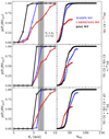 |
Fig. 1 Left column: probability of the injected periodic signal at Pc = 8.962 days existing in synthetic RV time-series, as a function of the injected semi-amplitude Kc with time-sampling identical to the published HARPS WF (C17a), the published CARMENES WF (S18), or their joint WF. Three sets of synthetic RV time-series are considered and contain K2-18c only (top row), K2-18b and c (middle row), or both planets plus a GP correlated noise model of stellar activity(bottom row). The shaded vertical region highlights the MAP and 1σ measured value of Kc = 4.63 ± 0.72 m s−1 from C17a. Right column: probability of the injected periodic signal at Pc existing in synthetic RV time-series, with fixed Kc = 4.63 m s−1, as a function of the number of RV measurements. |
2.2 Identifying anomalous CARMENES observations
We recall that the periodic signal from the proposed planet K2-18c at Pc = 8.962 days was not seen with a low false alarm probability in the GLSP of the full CARMENES time-series (S18). This is confirmed in the first panel of Fig. 2, although a small (albeit non-significant) hint of the ~9-day signal is visible. In computing the GLSP, the CARMENES RVs are weighted by the inverse square of their respective measurement uncertainties. As a brief experiment, we considered what the effect of adopting a uniform weighting on each RV (i.e. unweighted) would have on the probability of the 9-day signal. As can be seen in the second panel of Fig. 2, the 9-day signal becomes much more significant when using a uniform weighting. For comparison, the probability of the 9-day signal in the HARPS GLSP varies only weakly between the weighted and unweighted conventions (see bottom row of Fig. 2). This suggests that the 9-day signal does exist within the CARMENES RV dataset despite only appearing with significance when using an unconventional–and incorrect–method of computing the GLSP.
The sudden appearance of the 9-day periodic signal in the CARMENES RV suggests that some anomalous measurements may be partially responsible for the signal’s suppression to the extent that it becomes buried in the noise of the full CARMENES GLSP. If the number of such anomalous measurements is small compared to the full size of the dataset, then we can justify the removal of those measurements to measure the 9-day signal with CARMENES given our strong prior evidence for the signal from HARPS (C17a). We proceed by calculating the probability of Pc existing within various subsets of the full CARMENES time-series via leave-one-out cross-validation. In each of the 58 considered subsets, we omit a single unique measurement, compute the GLSP of the remaining 57 RVs, and isolate the probability of Pc existing within the data using an identical method to what was used in Sect. 2. The resulting probabilities of Pc as a function of the epoch of the omitted measurement are shown in Fig. 3.
In Fig. 3 we identify three anomalous RVs via a visual σ-clip7. We note that we refer to these measurements as anomalous as their inclusion versus their omittance clearly results in a significant reduction in p(Pc|RV) which is notseen for the majority of the CARMENES RVs. These measurements have associated RV uncertainties that are comparable to the mean CARMENES RV measurement uncertainty and thus have a significant effect on the probabilities of the periodicitiessampled in the GLSP. The removal of these three anomalous measurements and the recalculation of the GLSP using the proper RV weighting is shown in the third panel of Fig. 2. The 9-day periodic signal is now clearly seen at high probability. Clearly the strategic removal of just 3 out of 58 CARMENES RVs enhances the Pc periodic signal. Thus, we have significant preliminary evidence for the existence of the proposed planet K2-18c at ~ 9 days from the GLSP of the remaining 55 CARMENES RVs.
S18 provided their contemporaneous spectroscopic time-series of the CARMENES “full”, blue, and red RVs, as well as time-series of the chromospheric Hα index and the three CaII infrared triplet line indices. Inspection of these time-series does not reveal any obvious reason for why the three measurements identified in Fig. 3 significantly suppress the 9-day signal. We shared this result among the CARMENES team members who were also unable to identify any potential causes of the anomalous nature of these measurements after inspecting the measured RVs in individual orders. Therefore, at this time we are unable to explain the cause of the anomalous nature of these three measurements.
An exercise similar to that shown in Fig. 3 was also conducted using the HARPS RVs, the results of which are not presented here because the removal of individual HARPS RVs did not result in any significant changes to the probability of Pc existing within the reduced dataset; i.e. all values of p(Pc|RVHARPS) were close to 100% with a small rms of ~6%. The discrepancy between HARPS and CARMENES in this regard may be because the 9-day signal is less suppressed by the HARPS WF compared to the CARMENES WF (see Fig. 1) or because the HARPS WF contains more measurements and is thus less sensitive to the removal of individual measurements. The latter scenario highlights the need to obtain large NRV when searching for small planets whose RV semi-amplitudes are comparable to the RV measurement precision. This result has also been noted in simulations of “blind” RV searches (e.g. Cloutier et al. 2018) that strongly advocate for “more RVs per star” rather than “more stars with fewer RVs per star” in order to maximize future discoveries of small RV planets.
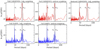 |
Fig. 2 Bayesian generalized Lomb–Scargle periodograms for various subsets of the published CARMENES and HARPS RVs with one of a pair of possible weighting schemes. The details of the time-series shown in each panel are annotated above the panel. The three dashed vertical lines depict the orbital period of the proposed non-transiting planet K2-18c (Pc = 8.962 days), the orbital period of the known transiting planet K2-18b (Pb = 32.93963 days), and the photometric stellar rotation period (Prot = 38.6 days). The Pc signal posited to be due to a second, non-transiting planet is seen at high relative probability in all but the full CARMENES RV time-series from S18 with a |

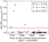 |
Fig. 3 Probability of the proposed K2-18c periodic signal Pc = 8.962 days existing within the CARMENES RV dataset from S18 but with a single measurement omitted via leave-one-out cross-validation. The abscissa depicts the observation epoch of each omitted RV measurement. The solid horizontal line depicts the 1σ dispersion of the probabilities. The three measurements which lie above the 1σ line significantly suppress the probability of Pc and are henceforth treated as anomalous. |
3 Chromatic dependence of the 9-day signal with HARPS
In addition to the RV variations derived from the 42 CARMENES visible orders, S18 also derived RVs from the first and second halves of these orders spanning 561–689 and 697–905 nm, respectively. Signal variations between these blue and red RVs may suggest that the nature of these signals as arising from stellar activity or from achromatic dynamical influences from planetary companions. Fluctuations in the strength of the 9-day signal in the CARMENES RVs helped lead S18 to conclude that the signal is due to stellar activity because of its apparent wavelength dependence. However, this evidence does not rule out the possibility that instead the 9-day signal is planetary in nature and appears to vary between the blue and red RVs because its suppression by activity is chromatically variable.
Similar to the method used by S18, here we compute the chromatic HARPS RVs to investigate the dependence of the 9-day signal strength with wavelength. The method used to derive these RVs at each observation epoch is detailed in Sect. 2.1 of C17a and is based on the methodology from Astudillo-Defru et al. (2015). The HARPS RVs are re-derived in each of the 72 HARPS orders although we restrict our analysis to orders redder than 498 nm where the signal-to-noise ratio (S/N) per spectral order is sufficient to reach a σRV per order ≲ 30 m s−1. The RVs derived from the remaining 34 orders are then grouped into blue and red orders whose weighted mean is used to compute the blue and red HARPS RVs. Our chromatic HARPS RVs span uneven wavelength ranges of 498–594 and 618–688 nm such that the resulting median RV measurement precision of ~ 7 m s−1 is comparable between the two sets of RVs. We note that the wavelength domain spanned by the red HARPS RVs is approximately equal to the redder half of the blue CARMENES wavelength domain.
The GLSPs of the blue and red HARPS RVs are shown in Fig. 4. In both GLSPs the ~9-day signal is discernible along with the forest of peaks around Pb and the stellar rotation period due to aliasing from the HARPS WF (cf. Fig.2 in C17a). Most notably, the probability of the 9-day peak is significantly greater in the HARPS red RVs than in the blue. This is expected if the 9-day signal is indeed due to a planet whose signalstrength is achromatic, whereas stellar activity arising from the temperature contrast of active regions is expected to increase bluewards (Reiners et al. 2010), thus degrading the S/N of the planetary signal in the blue RVs relative to the red. As such, if the 9-day signal originated from stellar activity rather than from a planet, one would expect the 9-day periodic signal to be stronger in the blue RVs, which it is not. Instead the rms of the blue RVs is slightly greater than in the red (7.8 m s−1 compared to 6.9 m s−1) even though each set of chromatic RVs has a comparable S/N. We note that this excess dispersion in the blue HARPS RVs is only marginal given the star’s moderate activity level (~ 2.7 m s−1; C17a; S18) which is less than RV measurement precision in either the blue or red HARPS RVs (~ 7 m s−1). The stronger activity level seen in the blue is likely responsible for the decreased significance of the 9-day signal and the enhanced probability at the stellar rotation period compared to the red.
Furthermore, we include the GLSP of the blue minus red RVs (see Fig. 4). The 9-day signal is significantly suppressed, whereas some residual probability close to the stellar rotation period persists along with some residual probability near Pb due to the aliasing of Prot by the HARPS WF. The suppression of the 9-day signal in the differential RVs is indicative of its achromatic nature (i.e. a dynamical signal), whereas the differing signal strength of RV activity in the blue and red RVs results in some residual power close to Prot. This furthersupports the planetary interpretation of the 9-day signal.
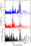 |
Fig. 4 Bayesian generalized Lomb–Scargle periodograms of the blue (top panel), red (middle panel), and HARPS RVs and their difference (bottom panel). The three dashed vertical lines depict the orbital period of the planets K2-18b and c (Pc ~ 9 days), and the photometric stellar rotation period. The 9-day signal is seen in the first two time-series, but at a lower probability in the blue likely due to the higher levels of stellar activity in that wavelength regime. The 9-day signal is suppressed in the GLSP of the RV difference, while some residual probability close to Prot continues topersist due to the incomplete removal of stellar activity. |
4 Temporal dependence of the 9-day signal with HARPS
In addition to the proposed chromatic dependence of the 9-day signal, S18 addressed the possibility that the 9-day signal strength also varies with time. This was posited based on the increased strength of the 9-day peak in the GLSP of the second half of the CARMENES RVs compared to the first. However, as was shown in Sect. 2.2, three anomalous CARMENES RVs exist in the first half of the CARMENES WF that significantly suppress the 9-day signal in the GLSP. This naturally explains why a stark increase in the 9-day signal strength was seen in the latter half of the CARMENES WF, and shows why it is not due to temporal variability in the stellar activity.
To further investigate the dependence of the 9-day signal on activity with HARPS, we can consider HARPS activity indices and the probability of the 9-day signal in each HARPS observing season separately. To extend the investigation of the temporal dependence of the 9-day signal, we obtained 31 additional HARPS spectra of K2-18 (i.e. in addition to the 75 presented in C17a). These new spectra extend the full HARPS baseline from April 2015 (BJD = 2 457 117.5) to July 2018 (BJD = 2 458 307.5). The method used to derive the stellar RVs at each observation epoch is detailed in Sect. 2.1 of C17a. The full set of 106 HARPS RVs are provided in Table A.1.
The full HARPS time-series is spanned by three separate observing seasons containing NRV ≥ 22. The GLSPs of the HARPS RVs in each observing season are shown in Fig. 5. Although the 9-day signal is visible in each GLSP, its probability relative to the surrounding continuum is seen to increase with time from early 2016 to mid-2018. If the 9-day signal is planetary in nature rather than due to stellar activity, then we would expect the K2-18 activity level to decrease with time thus enhancing the 9-day signal in the GLSP as the activity level subsides. Next we show that this is indeed the case.
To characterize the temporal variability of the K2-18 activity level, we compute the strength of the sodium doublet activity index (Na D) in all HARPS spectra following Astudillo-Defru et al. (2017). The Na D time-series is shown in the lower panel of Fig. 5. In particular we focus on the peak-to-peak amplitude A and rms of the Na D measurements in each observing season. In doing so we see that the amplitude of the variation in the Na D activity index and its rms both decrease across subsequent observing seasons. Specifically, we find that A = 0.0117 in the first observing season and drops to 0.0023 after ~26 months. Similarly, the Na D rms drops from 0.0027 to 0.0006 over the same time interval. These diagnostics indicate that the level of stellar activity is indeed decreasing with time and thus supports the planetary interpretation of the 9-day signal. A similar trend of increasing activity is also observed when considering other activity indicators such as the Hα index, although its time-series is not depicted in Fig. 5.
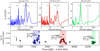 |
Fig. 5 Top row: Bayesian generalized Lomb–Scargle periodograms of the HARPS RVs in the three observing seasons annotated above each panel. The vertical dashed lines depict the orbital period of the proposed non-transiting planet K2-18c (Pc = 8.962 days), the orbital period of the known transiting planet K2-18b (Pb = 32.93963 days), and the photometric stellar rotation period (Prot = 38.6 days). Bottom row: sodium doublet time-series as measured by HARPS. The coloured regions/markers are indicative of the epochs used to compute each RV GLSP in theupper row. The annotation group adjacent to each observing season depicts the Na D peak-to-peak amplitude A, the NaD rms, and the number of measurements within that observing season. These A and rms diagnostics indicate that the level of stellar activity is decreasing with time, while the Pc signal is simultaneously becoming more prominent. |
5 Simultaneous RV modelling of planets and correlated noise
In the era ofultra-precise RV spectrographs whose inherent stability often operates below the photon-noise limit, RV detections of small planets suchas K2-18c are limited by nuisance signals from stellar activity. Numerous techniques have been tested to mitigate the effects of stellar activity whose amplitude and quasi-periodic temporal variability can mask and/or mimic planetary signals. Such techniques include linear correlations with contemporaneous activity indicators (e.g. Boisse et al. 2009), pre-whitening (e.g. Queloz et al. 2009), parametric modelling of stellar surface features (e.g. Dumusque et al. 2014), and sine wave fitting such as that used in S18. The main issue with this last technique is that the rotationally modulated activity in photometry and in RVs is not strictly periodic as the finite lifetimes of active regions, along with their variable sizes, contrasts, and spatial distributions will introduce a quasi-periodic component. This is especially true when RV time-series span many stellar rotation cycles. Incomplete models can result in the miscalculation of planetary parameters and the marginalization of coherent signals (e.g. additional planets) that are required to properly interpret the observed RV variations. When modelling RVs it is therefore crucial to include a flexible model that can account for stochastic variations in stellar activity. This is effectively done in a non-parametric way using GP regression simultaneously with planetary models (i.e. Keplerians), thus ensuring self-consistent solutions between planets and stellar activity. Furthermore, GP modelling fits within a Bayesian formalism as a single GP, which describe the temporal covariance between RV measurements with a single set of hyperparameters, is itself a prior distribution of functions whose mean represents the “best-fit” activity model (Haywood et al. 2014; Faria et al. 2016; Cloutier et al. 2017b). Here we analyse a variety of RV time-series from either the HARPS (C17a) or CARMENES (S18) spectrographs using a model that includes one or two planets plus a correlated noise component from stellar activity in the form of a GP regression model.
Our full two-planet model with observations taken by a single spectrograph contains 16 model parameters: the systemic velocity γ, an additive scalar jitter s, four quasi-periodic GP hyperparameters {a, λ, Γ, PGP}, and five Keplerian parameters per planet  . For cases in which we combine observations from HARPS and CARMENES, we treat their activity models as separate GPs (e.g. Grunblatt et al. 2015) owing to their unique systematics, the chromatic dependence of stellar activity, and each spectrograph’s distinct wavelength coverage. In this case, all GP hyperparameters are common between the two GP models with the exception of the additive jitter and the covariance amplitude. When modelling the joint HARPS+CARMENES time-series, we therefore have 19 model parameters.
The GP regression models of stellar activity are trained on the star’s precision K2 photometry. The apparent photometric variability, from which the photometric stellar rotation period was measured (PRV = 38.6 days; C17a), is sensitive to photospheric active regions which also have an observable manifestation in the RVs with common covariance properties. However, we note that photometry is only weakly sensitive to chromospheric plages which also contribute to RV activity signals, at least in Sun-like stars (Haywood et al. 2016). We use the K2 photometry to train our GP stellar activity models to ensure that the mean GP model from the simultaneous planet + activity modelling is representative of stellar activity and does not settle into a solution that describes other temporally correlated signals (e.g. non-transiting planets) by restricting the PGP to Prot or one of its low-order harmonics. By training our GP on ancillary time-series we empirically constrain the covariance structure of the activity signal and use the posterior probability density functions (PDFs) of the GP hyperparameters from training as priors during the RV modelling stage (see Table 1).
In these analyses we sample the posterior PDFs of the RV model parameters given an input dataset via Markov chain MonteCarlo (MCMC) simulations. All simulations are run using the affine-invariant MCMC ensemble sampler emcee (Foreman-Mackey et al. 2013). All model parameters are initialized around their MAP values with 1σ dispersions from C17a. The adopted model parameters are consistent between the various time-series considered and are summarized in Table 1. In each MCMC simulation we manually monitor the acceptance fraction and ensure that it always lies between 20 and 50% for both the burn-in phase and throughout the actual posterior PDF sampling.
Summary of the RV model parameter priors used for all models throughout this study.
5.1 CARMENES RVs
Here we model the subset of the CARMENES-visible RVs presented in S18 which are known to not result in the anomalous suppression of the 9-day signal. We consider two RV models, each containing a quasi-periodic GP regression model of stellar activity. The first model contains only one planetary signal from the confirmed transiting planet K2-18b, while the second model includes the second planet K2-18c at ~9 days. The RVs and GLSPs are plotted in Fig. A.1 for both the one- and two-planet models after iteratively removing the MAP models of activity and planetary signals.
In the one-planet model of the 55 CARMENES RVs, the GP activity model has a covariance amplitude of 7.5 m s−1 that is greater than the sinusoidal amplitude of 2.7 m s−1 measured by S18 on nearly the same dataset. Based on the GLSP of K2-18b (i.e. with activity removed), it is clear that although the activity model has a large amplitude, it fails to model the 9-day signal. The GLSP of the residuals following the removal of activity and K2-18b (Kb= 3.61 ± 0.82 m s−1) clearly exhibits a strong periodic signal at ~9 days hintingat the existence of an additional signal that is unmodelled when assuming a one-planet model.
The stellar activity in the two-planet model has a similarly large covariance amplitude of 8.2 m s−1. However, the only significant signal in the GLSP of the RV activity is at the stellar rotation period. Similarly, the GLSP of K2-18b (Kb= 2.91 ± 0.88 m s−1) only exhibits a significant signal at Pb, and the GLSP of K2-18c (Kc = 2.31 ± 0.76 m s−1) exhibit a strong signal at ~9 days with a somewhat weaker signal at ~5.5 days. The GLSP of the residuals following the removal of both planets and activity only shows a significant residual probability at ~ 5.5 days, which only arises after the removal of activity and K2-18b (cf. panels of O–C and K2-18c in Fig. A.1). The nature of this signal is less obvious; unlike the 9-day signal, it does not appear with enough significance in either GLSP of the HARPS or CARMENES RVs prior to the removal of any modelled signals (see Fig. 2). One possible explanation is that the ~ 5.5-day signal arises from an alias of Pc with the CARMENES WF which exhibits excess power close to the baseline duration of ~ 189 days. Using the standard formula to compute the alias frequency from the signal and WF frequencies (i.e. falias = fsignal + nfWF), and setting fsignal = 1∕8.997 days−1 and fWF = 1∕189 days−1, we find an aliased periodicity at ~5.56 days when n = 13. Given the high-order n required to identify an aliased periodicity that is seemingly consistent with the excess probability at ~ 5.5 days, we do not claim that this WF alias explains the signal’s origin and similarly we cannot discard the possibility that the 5.5-day signal comes from an additional planet that has not yet been detected. More RV data are required to investigate the source of this signal. In Sect. 5.5 we perform a model comparison considering the possibility that the 5.5-day signal is due to a third planet in the system.
5.2 All HARPS RVs
In Sect. 4 we presented 31 new HARPS RVs to investigate the temporal variability of the 9-day signal. Hence, the full HARPS WF has been extended to over a year past the previously most recent published HARPS measurement for this system (C17a) and now contains 106 RV measurements. Here we model the full HARPS time-series in the same way as was done for the CARMENES RVs in Sect. 5.1. The RVs and GLSPs are plotted in Fig. A.2.
In the one-planet model the GP activity model has a covariance amplitude of 2.3 m s−1, comparable to the MAP Kb = 2.75 ± 0.66 m s−1. Similar to the one-planet model of the CARMENES RVs, the activity model fails to account for the high probability of the 9-day signal. The 9-day peak continues to persist following the removal of the K2-18b Keplerian.
In the two-planet model, the GP activity model has a somewhat larger covariance amplitude compared to the one-planet model: 4.18 m s−1. This amplitude is comparable to the MAP semi-amplitudes of the two planets (Kb = 3.32 ± 0.60 m s−1, Kc = 3.71 ± 0.57 m s−1) and, given the proximity of the stellar rotation period to Pb and aliases of the two aforementioned periods with the WF (S18), the activity model only partially suppresses the GLSP probabilities between ~30 and 50 days. It is also clear that when the mean activity model and only a single planet are removed, the only remaining signal at high probability is that of the remaining planet at 9 days. Furthermore, it is clear that there are no residual signals at high probability when all modelled signals are removed. Most notably, a probability peak at ~5.5 days, as was seen in the CARMENES residuals with a two-planet model (Fig. A.1), is visible but only at the level of the noise.
5.3 Joint HARPS+CARMENES RVs
Here we model the joint RV time-series of the 106 HARPS plus the 55 CARMENES RVs. The RVs and GLSPs are plotted in Fig. A.3. In the one-planet model, the covariance amplitude of the HARPS and CARMENES stellar activity models are 1.5 and 5.5 m s−1, respectively.These values are each slightly smaller than the covariance amplitudes measured when considering each spectrograph’s time-series individually but their ratio is nearly preserved. Similar to either spectrograph’s individual RV analysis in the presence of a one-planet model, the GLSP of the residuals following the removal of K2-18b (Kb= 3.00 ± 0.50 m s−1) and activity exhibits a strong periodic signal at ~9 days which again hints at the existence of an additional planetary signal.
The stellar activity covariance amplitudes in the two-planet model are comparable to that in the one-planet model, i.e. 3.0 and 5.5 m s−1 for HARPS and CARMENES, respectively. The corresponding GLSP of the RV activity is reminiscent of the one-planet RV activity GLSP with the exception that the inclusion of two modelled planets (Kb= 2.75 ± 0.43 m s−1, Kc = 2.76 ± 0.41 m s−1) drastically reduces the probability of the 9-day signal. Indeed, in the GLSP of K2-18c, the strongest signal is at ~ 9 days with only a hint of the ~5.5-day signal that was seen in CARMENES. In both the GLSP of the HARPS and joint RV residuals following the removal of both planets and activity (see Figs. A.2 and A.3), the ~5.5-day signal is notseen at high probability, which suggests that the signal is not physical and instead arises stochastically as a by-product of the CARMENES WF.
5.4 Overlapping HARPS and CARMENES window functions
For a maximal one-to-one comparison we can compare the RV model analyses and GLSP structures in the subsets of the HARPS and CARMENES RVs that are restricted to the 138 days from February 2 to June 20, 2017. Between these dates the HARPS and CARMENES WFs overlap such that we have approximately contemporaneous RVs taken with each spectrograph. By only considering the observations taken throughout the overlapping time span we minimize our sensitivity to temporal variations in stellar activity whose properties may vary between successive observing cycles. The overlapping WF contains 35 HARPS and 50 CARMENES RVs. One of the CARMENES RVs in the overlapping window was found to anomalously suppress the ~9-day signal in Sect. 2.2, so we discarded it and were left with 49 CARMENES RVs. The RVs and GLSPs are plotted in Fig. A.4.
In the one-planet model the covariance amplitudes are equivalent with each spectrograph (i.e. 2.0 m s−1) and are notably small compared to the previously analysed time-series. This may be due to the lack of a long-term near-linear trend in the stellar activity over the short time span considered here. The corresponding activity model appears close to flat indicating that the RV activity has only weak structure over this relatively short time span. The low activity amplitude also results in a low probability at Prot and the activity GLSP being dominated by the 9-day signal, which is effectively unmodelled when only one planet is considered. We measure Kb = 3.96 ± 0.73 m s−1, which along with the activity model reveals the residual 9-day signal and the ~5.5-day signal that was seen in the CARMENES residuals.
In the two-planet model the covariance amplitudes are nearly identical to the one-planet model (2.0 m s−1) and therefore exhibit a similar featureless structure. The small covariance amplitudes of the activity models result in the activity GLSP containing primarily noise. Comparatively, the GLSPs of the modelled planets (Kb = 3.59 ± 0.62 m s−1, Kc = 2.65 ± 0.58 m s−1) are dominated by their respective periodicities with the ~ 5.5 days signal appearing in the GLSP of K2-18c, albeit at a much lower probability than the 9-day signal. However, in the residual GLSP, the ~5.5-day signal is largely suppressed after removing K2-18c.
5.5 Model comparison
The detection of exoplanets in RV data is fundamentally based on whether or not the input dataset favours the existence of the planet of interest. This is typically done within a Bayesian framework wherein the fully marginalized likelihoods (i.e. the evidence) of competing models (i.e. one versus two planets) are computed and used for model comparison. In this formalism, a planet is said to be detected if the evidence for the (n + 1)-planet model is significantly larger than the evidence for a model containing n planets. Here we calculate the model evidence for the purpose of model comparison and use the resulting values to determine whether the putative RV planet K2-18c is favoured by the various time-series considered.
Each model’s Bayesian evidence is approximated using the estimator from Perrakis et al. (2014) and the marginalized posterior PDFs from our MCMC analyses as importance samplers. The Perrakis et al. (2014) estimator is known to result in quantitatively similar results to other more robust but computationally expensive methods (e.g. nested samplers; Nelson et al. 2018). Model comparison requires that all common model parameters between competing models be drawn from identical prior distributions, which are listed in Table 1. Our Bayesian evidence estimates are reportedin Table 2 for both the one- and two-planet models and for all input time-series considered.
Also included in Table 1 are the 2-1 Bayes factors (i.e. evidence ratios) of the two-planet model relative to the one-planet to determine whether the second planet K2-18c is favoured or disfavoured by the corresponding time-series. Overall, we find that the explicit values of the Bayesian evidence favour the two-planet model for all the time-series considered. However, the dispersion in calculated evidence values when using various methods of calculation are known to vary by factors of ≳ 102 depending on the complexity of the model (i.e. the number of planets; Nelson et al. 2018). We recall that the simplest model considered in this study is not the zero-planet model as we know from the transit light curves that K2-18b exists at ~ 33 days. Effectively, we are therefore only tasked with detecting one new RV planet rather than two. But given the caveat that uncertainties in the calculated evidence can be of the order of 102, we require that the evidence ratio of the two-planet model to the one-planet model must be ≥ 102 for the second planet K2-18c to be detected. Under this condition there are two instances in which K2-18c is not detected. The first occurs with the full set of the 58 CARMENES RVs from S18 in which K2-18c is not detected due to the three anomalous measurements identified in Sect. 2.2. This result is consistent with the null detection of K2-18c with these data in S18. However, the 2-1 Bayes factor for CARMENES alone exceeds 102 following the removal of the three measurements mentioned above. The second occurs because the blue CARMENES RVs only weakly favour a second planet which can be attributed to the increased RV rms at these shorter wavelengths8. This trend is seen again in the blue and red HARPS RVs for which a second planet is more strongly favoured by the red RVs where the RV rms is smaller. The increased measurement uncertainty for CARMENES in the blue hides planetary signals and makes the inference of their presence less certain given the correspondingly low data likelihoods.
We recall the ~5.5-day signal seen in the K2-18c and residual GLSPs of the RV time-series containing CARMENES data in Figs. A.1, A.3, and A.4. As a test of the potential planetary origin of this signal we first ran an MCMC on the CARMENES RVs as it is there that the residual 5.5-day signal exhibited the highest probability in the GLSP following the removal of K2-18b, c, and stellar activity. As we did for the one- and two-planet models, we then estimate the evidence of this three-planet model using the estimator from Perrakis et al. (2014) and compare it to the two-planet, model for the same input time-series. For the third planet we adopt identical priors to that of K2-18c (see Table 1) with the exception of the planet’s orbital period and time of mid-conjunction which are modified to  days and
 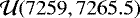 BJD-2 450 000, respectively. The resulting ln evidence for the two- and three-planet models are −165.0 and −162.4, respectively. The corresponding 3-2 Bayes factor is ~7, implying that the three-planet model including a planet at ~ 5.5 days is not significantly favoured over the two-planet model. By a similar exercise, using the full joint HARPS+CARMENES time-series yields a 3-2 Bayes factorof ~0.8. Therefore, by the effective accounting of the 5.5-day periodic signal by our K2-18c models in Figs. A.2–A.4, and the disfavourability of the three-planetmodel compared to the model containing just two planets, we conclude that a third planet at ~ 5.5 days is not detected in the available RV data, but its signal origin may be alluded to with additional RV monitoring.
Marginal likelihood estimations and Bayes factors for various RV datasets and models.
6 Discussion and conclusions
We have conducted a systematic reanalysis of the published HARPS (C17a) and CARMENES (S18) RVs of the transiting planet host K2-18 to identify the source of the apparent 9-day signal which prior to this study had only been seen in the HARPS dataset. We have also included an additional set of 31 new HARPS RVs to investigate the temporal dependence of the 9-day signal and to improve the measurement precision of planet parameters. Our main conclusions are the following:
- 1.
The CARMENES window function is somewhat detrimental to the detection of an injected 9-day Keplerian signal compared to the HARPS window function, in that the injected signal is seen at a lower probability in the generalized Lomb-Scargle periodogram (GLSP) when using the CARMENES window function.
- 2.
The cause of the non-detection of the 9-day signal in S18 was shown to result from three anomalous CARMENES measurements; when they are removed the existence of the 9-day signal is revealed in the GLSP of the remaining 55 RVs.
- 3.
We computed two sets chromatic HARPS RVs. The 9-day signal is seen in both time-series and at a significantly higher probability in the red HARPS RVs where stellar activity is weaker. This supports the planetary interpretation of the 9-day signal.
- 4.
The 9-day signal is retrieved with HARPS in each of its three observing seasons separated by ~1 year. The probability of the 9-day signal increases with time simultaneously with a decrease in the level of stellar activity as probed by the Na D activity index. This further supports the planetary interpretation of the 9-day signal.
- 5.
We adopt a non-parametric stellar activity model to account for stellar variability over the multiple stellar rotation cycles spanned by the observations, and simultaneously model activity and planetary signals. This results in self-consistent planet solutions and the ability to compare one- and two-planet models on equal grounds.
- 6.
In all the considered times-series, the Bayesian model evidence favours a two-planet model over the one-planet model which includes K2-18c at ~9 days.
By the points listed above, we have obtained compelling evidence for the planetary nature of the 9-day signal seen in HARPS and in the reduced CARMENES RV time-series. It is important to highlight the importance of basing RV planet detections on robust Bayesian model comparison tests rather than basing those detections solely on periodogram false alarm probabilities (FAPs) which can vary stochastically and are highly sensitive to variations in the input time-series (e.g. weighting schemes). Although significant peaks in a GLSP are useful for the initial identification of periodic signals in unevenly sampled time-series, conclusions regarding their actual existence and origin should not be made solely based on their FAP. Accurate and simultaneous modelling of all signals present in a time-series is required to determine accurate model parameters of planets and activity. Furthermore, Bayes factors – or the ratio of the competing models’ fully marginalized likelihoods – are robust model comparison tools which marginalize over all prior information about models with competing numbers of planets and penalize overly complicated models. In this way they are optimally suited to the detection confirmation of periodic planetary signals.
In our re-analysis of the joint HARPS+CARMENES RVs we have measured the most likely Keplerian solution to each planet’s orbit. By including all available RV observations of the K2-18 system (excluding those known to be anomalous), we have obtained the most precise planetary solutions for K2-18 to date. The point estimates of the two-planet model parameters resulting from this analysis are presented in Table A.2. As a sanity check we can compare the resulting marginalized posterior PDFs for parameters of interest between the individual HARPS, CARMENES, and their joint RV time-series. In this way we can ensure that the planetary solutions from the time-series of the two spectrographs are consistent with each other and with their joint time-series. For instance, we compare the resulting marginalized poster PDFs of Kb and Kc obtained with each time-series in Fig. 6. It is evident that the MAP Kb solutions are nearly equivalent when measured with any of the three time-series. Similarly, MAP Kc values are consistent at the 1σ level, albeit with more dispersion than the Kb PDFs giventhe comparatively large uncertainties in the K2-18c ephemeris.
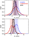 |
Fig. 6 1D marginalized posterior PDFs of the K2-18b and c semi-amplitudes from analyses of the full HARPS (blue), the reduced CARMENES (red), and their joint (black) RV time-series. The dashed vertical lines and shaded regions depict the maximum a posteriori values and 1σ confidence intervals respectively. All Kb and Kc values are consistent at the 1σ level which is approximated by each PDF’s 16th and 84th percentiles. |
6.1 Improved stellar parameters based on Gaia DR2
To map the observable transit and RV parameters to physical planetary parameters we must first characterize the host star. Specifically, we can exploit the exquisite precision of the Gaia DR2 to improve the stellar mass and radius of K2-18.
Firstly, the K2-18 stellar mass is computed from the M dwarf mass-luminosity relation (MLR) from Benedict et al. (2016). The analytical MLR based on absolute K-band magnitudes is favoured over the V -band whose dispersion about the relation is twice that in the K-band. The distance modulus is calculated from the precision Gaia DR2 stellar parallax (p = 26.299 ± 0.055 mas; Gaia Collaboration 2018) to be μ = 2.900 ± 0.005, where we have added the 30 μas systematic offset in the measured parallax as noted in Lindegren et al. (2018). By propagating errors in the K2-18 K-band magnitude (K = 8.899 ± 0.019; Cutri et al. 2003), the distance modulus, and the MLR coefficients, we find an absolute K-band magnitude of MK = 5.999 ± 0.020 and a corresponding stellar mass of Ms = 0.495 ± 0.004 M⊙.
From the stellar mass we are able to derive the stellar radius using the empirical mass-radius relationship (MRR) for M dwarfs from Boyajian et al. (2012). By propagating the uncertainties in the M dwarf MRR coefficients we compute the K2-18 stellar radius to be Rs = 0.469 ± 0.010 R⊙. We note that both the updated stellar mass and radius, which are based on the stellar parallax, are considerably larger than the spectroscopically derived values of 0.359 ± 0.047 M⊙ and 0.411 ± 0.038 R⊙ (Benneke et al. 2017). The new mass and radius values are inconsistent with their previous values at the levels of 2.9σ and 1.5σ, respectively. This is the direct result of the increased K2-18 distance from Gaia (38.025 ± 0.079 pc) compared to its previously measured distance (34 ± 4 pc) and will have important implications for the derived physical parameters of both K2-18b and c. We also note the improved fractional uncertainties on the updated stellar mass and radius of 0.8 and 2.1%, respectively, compared to the previous fractional uncertainties of 13.1 and 9.2%.
6.2 Precise planetary parameters
The improved stellar parameters, along with our joint HARPS+CARMENES RV analysis, provide the most precise set of planetary parameters for the planets K2-18b and c to date. Point estimates of the planetary parameters from our joint HARPS+CARMENES RV analysis are presented in Table A.2. In particular, we measure the precise mass and minimum mass of K2-18b and c, respectively, to be mp,b = 8.64 ± 1.35 M⊕ and mp,c sinic = 5.63 ± 0.84 M⊕.
The improved stellar radius also provides a more precise planetary radius given the measured rp,b ∕Rs value from Benneke et al. (2017). We find that rp,b = 2.711 ± 0.065 R⊕. From this we derive a planetary bulk density for K2-18b of ρp,b = 2.4 ± 0.4 g cm−3, thus making K2-18b inconsistent with either an Earth-like composition or a pure water-world (Zeng & Sasselov 2013). Prior to updating the mass and radius of K2-18b, neither of these scenarios could have been ruled out. It is now clear that at minimum, ~ 8% of the size of K2-18b (i.e. ~1382 km) must be attributed to an optically think gaseous atmosphere as evidenced by its low bulk density. The expected signal amplitude in transmission for a cloud-free hydrogen-dominated atmosphere (μ = 2) is  ppm, where H = kBTeq∕μmpg is the atmospheric pressure scale height, kB is the Boltzmann constant, Teq is the planet’s equilibrium temperature assuming an Earth-like Bond albedo, μmp is the assumed mean molecular weight, and g is the surface gravity (Kaltenegger & Traub 2009). For comparison, a well-mixed water-dominated atmosphere (μ = 18) has a transmission signal amplitude of ~18 ppm. Given the scale height of its extended gaseous envelop and its proximity to the solar system, K2-18b continues to represent an exciting opportunity to characterize a sub-Neptune-sized exoplanet receiving Earth-like insolation with upcoming space missions such as the James Webb Space Telescope and ARIEL.
Acknowledgements
R.C. thanks the anonymous referee and the CARMENES team, particularly P. Sarkis and T. Henning, for taking the time to read and comment on the manuscript during its editing phase and particularly the CARMENES team for investigating the potential causes of the anomalous CARMENES RVs. R.C. and K.M. acknowledge support for this work from the Natural Sciences and Engineering Research Council of Canada. N.A.D. acknowledges support from FONDECYT 3180063. X.B., J.M.A, and A.W. acknowledge funding from the European Research Council under the ERC Grant Agreement n. 337591-ExTrA. N.C.S. acknowledges the funding by FEDER – Fundo Europeu de Desenvolvimento Regional funds through the COMPETE 2020 – Programa Operacional Competitividade e Internacionalização (POCI), and by Portuguese funds through FCT – Fundaçãopara a Ciência e a Tecnologia in the framework of the projects POCI-01-0145-FEDER-028953 and POCI-01-0145-FEDER-032113, and from FCT and FEDER through COMPETE2020 to grants UID/FIS/04434/2013 and POCI-01-0145-FEDER-007672, PTDC/FIS-AST/1526/2014 and POCI-01-0145-FEDER-016886, and PTDC/FIS-AST/7073/2014 and POCI-01-0145-FEDER-016880.
Appendix A: Iterative radial velocity time-series and GLSP figures from Sect. 5
In Sect. 5 we considered a variety of RV datasets and models which included either one or two planets along with a GP regression model of stellar activity that had been trained on the star’s K2 photometry. The following figures depict the iterative RVs and GLSPs for each dataset and model. In each iteration we removed one or more coherent signals (i.e. planets or activity) to see if any residual periodicities persist for which additional model components may be required.
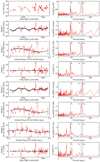 |
Fig. A.1 Results of our RV analysis of the 55 CARMENES RVs that are known not to significantly suppress the apparent 9-day signal seen with HARPS. The RV time-series and their corresponding GLSP are plotted in common rows for each coherent RV signal modelled (i.e. planets and stellar activity) in either a one- or two-planet model. The overplotted RV models are computed using the MAP model parameters from our MCMC analysis. The vertical dashed lines in the GLSPs are indicative of the MAP orbital periods for K2-18b and c and the photometric stellar rotation period. The first row depicts the raw RVs; the next three following rows present the results assuming a one-planet model (i.e. K2-18b); and the final four rows present the results assuming a two-planet model (i.e. K2-81b and c). The residual rms values assuming a one- and two-planet model are 3.84 and 3.57 m s−1, respectively. We find that the source of the residual ~5.5-day signal in thebottom GLSP is due to an alias rather than an unmodelled physical source (see text). |
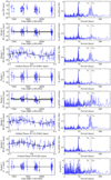 |
Fig. A.2 Similar to Fig. A.1, but for the full HARPS WF containing 106 RVs. The rms of the residual time-series assuming a one- and two-planet model are 4.68 and 3.93 m s−1, respectively.MAP RV models. GLSP periodicities. |
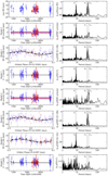 |
Fig. A.3 Similar to Fig. A.1, but for the 161 joint HARPS+CARMENES RVs. The HARPS and CARMENES RVs are plotted as blue and red markers, respectively. The phase-folded RVs depicting planetary signals are binned for clarity. The rms of the residual time-series assuming a one- and two-planet model are 4.51 and 3.82 m s−1, respectively.MAP RV models. GLSP periodicities. |
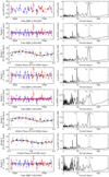 |
Fig. A.4 Similar to Fig. A.1, but for the 84 joint HARPS+CARMENES RVs obtained during the time interval in which the two spectrograph WFs overlap (February–June 2017). The HARPS and CARMENES RVs are plotted as blue and red markers, respectively. The phase-folded RVs depicting planetary signals are binned for clarity. The rms of the residual time-series assuming a one- and two-planet model are 4.26 and 3.62 m s−1, respectively.MAP RV models. GLSP periodicities. |
Full HARPS time-series from C17a and this work.
K2-18 model parameters from the HARPS+CARMENES joint RV analysis.
References
- Astudillo-Defru, N., Bonfils, X., Delfosse, X., et al. 2015, A&A, 575, A119 [NASA ADS] [CrossRef] [EDP Sciences] [Google Scholar]
- Astudillo-Defru, N., Forveille, T., Bonfils, X., et al. 2017, A&A, 602, A88 [NASA ADS] [CrossRef] [EDP Sciences] [Google Scholar]
- Benedict, G. F., Henry, T. J., Franz, O. G., et al. 2016, AJ, 152, 141 [NASA ADS] [CrossRef] [Google Scholar]
- Benneke, B., Werner, M., Petigura, E., et al. 2017, ApJ, 834, 187 [NASA ADS] [CrossRef] [Google Scholar]
- Boisse, I., Moutou, C., Vidal-Madjar, A., et al. 2009, A&A, 495, 959 [NASA ADS] [CrossRef] [EDP Sciences] [Google Scholar]
- Boisse, I., Bouchy, F., Hébrard, G., et al. 2011, A&A, 528, A4 [NASA ADS] [CrossRef] [EDP Sciences] [Google Scholar]
- Boyajian, T. S., von Braun, K., van Belle, G., et al. 2012, ApJ, 757, 112 [NASA ADS] [CrossRef] [Google Scholar]
- Cloutier, R., Astudillo-Defru, N., Doyon, R., et al. 2017a, A&A, 608, A35 [NASA ADS] [CrossRef] [EDP Sciences] [Google Scholar]
- Cloutier, R., Doyon, R., Menou, K., et al. 2017b, AJ, 153, 9 [NASA ADS] [CrossRef] [Google Scholar]
- Cloutier, R., Artigau, É., Delfosse, X., et al. 2018, AJ, 155, 93 [NASA ADS] [CrossRef] [Google Scholar]
- Cutri, R. M., Skrutskie, M. F., van Dyk, S., et al. 2003, 2MASS All Sky Catalog of Point Sources [Google Scholar]
- Dumusque, X., Boisse, I., & Santos, N. C. 2014, ApJ, 796, 132 [NASA ADS] [CrossRef] [Google Scholar]
- Faria, J. P., Haywood, R. D., Brewer, B. J., et al. 2016, A&A, 588, A31 [NASA ADS] [CrossRef] [EDP Sciences] [Google Scholar]
- Foreman-Mackey, D., Hogg, D. W., Lang, D., & Goodman, J. 2013, PASP, 125, 306 [CrossRef] [Google Scholar]
- Foreman-Mackey, D., Montet, B. T., Hogg, D. W., et al. 2015, ApJ, 806, 215 [NASA ADS] [CrossRef] [Google Scholar]
- Gregory, P. C. 2005, ApJ, 631, 1198 [NASA ADS] [CrossRef] [Google Scholar]
- Grunblatt, S. K., Howard, A. W., & Haywood, R. D. 2015, ApJ, 808, 127 [NASA ADS] [CrossRef] [Google Scholar]
- Hatzes, A. P. 2016, A&A, 585, A144 [NASA ADS] [CrossRef] [EDP Sciences] [Google Scholar]
- Haywood, R. D., Collier Cameron, A., Queloz, D., et al. 2014, MNRAS, 443, 2517 [NASA ADS] [CrossRef] [Google Scholar]
- Haywood, R. D., Collier Cameron, A., Unruh, Y. C., et al. 2016, MNRAS, 457, 3637 [NASA ADS] [CrossRef] [Google Scholar]
- Kaltenegger, L. & Traub, W. A. 2009, ApJ, 698, 519 [NASA ADS] [CrossRef] [Google Scholar]
- Lindegren, L., Hernández, J., Bombrun, A., et al. 2018, A&A, 616, A2 [NASA ADS] [CrossRef] [EDP Sciences] [Google Scholar]
- Mayor, M., Pepe, F., Queloz, D., et al. 2003, The Messenger, 114, 20 [NASA ADS] [Google Scholar]
- Montet, B. T., Morton, T. D., Foreman-Mackey, D., et al. 2015, ApJ, 809, 25 [NASA ADS] [CrossRef] [Google Scholar]
- Mortier, A., Faria, J. P., Correia, C. M., Santerne, A., & Santos, N. C. 2015, A&A, 573, A101 [NASA ADS] [CrossRef] [EDP Sciences] [Google Scholar]
- Nelson, B. E., Ford, E. B., Buchner, J., et al. 2018, ArXiv e-prints, [arXiv:1806.04683] [Google Scholar]
- Perrakis, K., Ntzoufras, I., & Tsionas, E. G. 2014, Comput. Stat. Data Anal. 77, 54 [CrossRef] [Google Scholar]
- Queloz, D., Bouchy, F., Moutou, C., et al. 2009, A&A, 506, 303 [NASA ADS] [CrossRef] [EDP Sciences] [Google Scholar]
- Quirrenbach, A., Amado, P. J., Caballero, J. A., et al. 2014, in Ground-based and Airborne Instrumentation for Astronomy V, Proc. SPIE, 9147, 91471F [Google Scholar]
- Rajpaul, V., Aigrain, S., & Roberts, S. 2016, MNRAS, 456, L6 [NASA ADS] [CrossRef] [Google Scholar]
- Rajpaul, V., Buchhave, L. A., & Aigrain, S. 2017, MNRAS, 471, L125 [NASA ADS] [CrossRef] [Google Scholar]
- Reiners, A., Bean, J. L., Huber, K. F., et al. 2010, ApJ, 710, 432 [NASA ADS] [CrossRef] [Google Scholar]
- Sarkis, P., Henning, T., Kürster, M., et al. 2018, AJ, 155, 257 [NASA ADS] [CrossRef] [Google Scholar]
- Zeng, L., & Sasselov, D. 2013, PASP, 125, 227 [NASA ADS] [CrossRef] [Google Scholar]
For example, the S-index, Hα index, full width at half maximum, and the bi-sector inverse slope of the spectral cross-correlation function.
Although periodicities at the second and third harmonics are not seen in the CARMENES RVs with comparable significance to that of the 9-day signal.
A strong periodic signal in the periodogram of the HARPS RVs at ~9 days, a 6.3σ semi-amplitude measurement, the favourability of a two-planet model by cross-validation model comparison (C17a).
3.60, 3.08, and 3.37 m s−1 for HARPS, CARMENES, and their joint time-series, respectively.
Nf = 75, 58, and 133 for HARPS, CARMENES, and their joint time-series, respectively.
For RV indices starting at 0, the three anomalous CARMENES RVs have indices 4, 6, and 14 (i.e. BJD-2 450 000 = 7759.69656, 7766.73773, 7817.51320).
7.5 m s−1 compared to 5.14 and 5.73 m s−1 in the full and red CARMENES RVs, respectively.
All Tables
Summary of the RV model parameter priors used for all models throughout this study.
Marginal likelihood estimations and Bayes factors for various RV datasets and models.
All Figures
|
Fig. 1 Left column: probability of the injected periodic signal at Pc = 8.962 days existing in synthetic RV time-series, as a function of the injected semi-amplitude Kc with time-sampling identical to the published HARPS WF (C17a), the published CARMENES WF (S18), or their joint WF. Three sets of synthetic RV time-series are considered and contain K2-18c only (top row), K2-18b and c (middle row), or both planets plus a GP correlated noise model of stellar activity(bottom row). The shaded vertical region highlights the MAP and 1σ measured value of Kc = 4.63 ± 0.72 m s−1 from C17a. Right column: probability of the injected periodic signal at Pc existing in synthetic RV time-series, with fixed Kc = 4.63 m s−1, as a function of the number of RV measurements. |
| In the text | |
|
Fig. 2 Bayesian generalized Lomb–Scargle periodograms for various subsets of the published CARMENES and HARPS RVs with one of a pair of possible weighting schemes. The details of the time-series shown in each panel are annotated above the panel. The three dashed vertical lines depict the orbital period of the proposed non-transiting planet K2-18c (Pc = 8.962 days), the orbital period of the known transiting planet K2-18b (Pb = 32.93963 days), and the photometric stellar rotation period (Prot = 38.6 days). The Pc signal posited to be due to a second, non-transiting planet is seen at high relative probability in all but the full CARMENES RV time-series from S18 with a |
| In the text | |
|
Fig. 3 Probability of the proposed K2-18c periodic signal Pc = 8.962 days existing within the CARMENES RV dataset from S18 but with a single measurement omitted via leave-one-out cross-validation. The abscissa depicts the observation epoch of each omitted RV measurement. The solid horizontal line depicts the 1σ dispersion of the probabilities. The three measurements which lie above the 1σ line significantly suppress the probability of Pc and are henceforth treated as anomalous. |
| In the text | |
|
Fig. 4 Bayesian generalized Lomb–Scargle periodograms of the blue (top panel), red (middle panel), and HARPS RVs and their difference (bottom panel). The three dashed vertical lines depict the orbital period of the planets K2-18b and c (Pc ~ 9 days), and the photometric stellar rotation period. The 9-day signal is seen in the first two time-series, but at a lower probability in the blue likely due to the higher levels of stellar activity in that wavelength regime. The 9-day signal is suppressed in the GLSP of the RV difference, while some residual probability close to Prot continues topersist due to the incomplete removal of stellar activity. |
| In the text | |
|
Fig. 5 Top row: Bayesian generalized Lomb–Scargle periodograms of the HARPS RVs in the three observing seasons annotated above each panel. The vertical dashed lines depict the orbital period of the proposed non-transiting planet K2-18c (Pc = 8.962 days), the orbital period of the known transiting planet K2-18b (Pb = 32.93963 days), and the photometric stellar rotation period (Prot = 38.6 days). Bottom row: sodium doublet time-series as measured by HARPS. The coloured regions/markers are indicative of the epochs used to compute each RV GLSP in theupper row. The annotation group adjacent to each observing season depicts the Na D peak-to-peak amplitude A, the NaD rms, and the number of measurements within that observing season. These A and rms diagnostics indicate that the level of stellar activity is decreasing with time, while the Pc signal is simultaneously becoming more prominent. |
| In the text | |
|
Fig. 6 1D marginalized posterior PDFs of the K2-18b and c semi-amplitudes from analyses of the full HARPS (blue), the reduced CARMENES (red), and their joint (black) RV time-series. The dashed vertical lines and shaded regions depict the maximum a posteriori values and 1σ confidence intervals respectively. All Kb and Kc values are consistent at the 1σ level which is approximated by each PDF’s 16th and 84th percentiles. |
| In the text | |
|
Fig. A.1 Results of our RV analysis of the 55 CARMENES RVs that are known not to significantly suppress the apparent 9-day signal seen with HARPS. The RV time-series and their corresponding GLSP are plotted in common rows for each coherent RV signal modelled (i.e. planets and stellar activity) in either a one- or two-planet model. The overplotted RV models are computed using the MAP model parameters from our MCMC analysis. The vertical dashed lines in the GLSPs are indicative of the MAP orbital periods for K2-18b and c and the photometric stellar rotation period. The first row depicts the raw RVs; the next three following rows present the results assuming a one-planet model (i.e. K2-18b); and the final four rows present the results assuming a two-planet model (i.e. K2-81b and c). The residual rms values assuming a one- and two-planet model are 3.84 and 3.57 m s−1, respectively. We find that the source of the residual ~5.5-day signal in thebottom GLSP is due to an alias rather than an unmodelled physical source (see text). |
| In the text | |
|
Fig. A.2 Similar to Fig. A.1, but for the full HARPS WF containing 106 RVs. The rms of the residual time-series assuming a one- and two-planet model are 4.68 and 3.93 m s−1, respectively.MAP RV models. GLSP periodicities. |
| In the text | |
|
Fig. A.3 Similar to Fig. A.1, but for the 161 joint HARPS+CARMENES RVs. The HARPS and CARMENES RVs are plotted as blue and red markers, respectively. The phase-folded RVs depicting planetary signals are binned for clarity. The rms of the residual time-series assuming a one- and two-planet model are 4.51 and 3.82 m s−1, respectively.MAP RV models. GLSP periodicities. |
| In the text | |
|
Fig. A.4 Similar to Fig. A.1, but for the 84 joint HARPS+CARMENES RVs obtained during the time interval in which the two spectrograph WFs overlap (February–June 2017). The HARPS and CARMENES RVs are plotted as blue and red markers, respectively. The phase-folded RVs depicting planetary signals are binned for clarity. The rms of the residual time-series assuming a one- and two-planet model are 4.26 and 3.62 m s−1, respectively.MAP RV models. GLSP periodicities. |
| In the text | |
Current usage metrics show cumulative count of Article Views (full-text article views including HTML views, PDF and ePub downloads, according to the available data) and Abstracts Views on Vision4Press platform.
Data correspond to usage on the plateform after 2015. The current usage metrics is available 48-96 hours after online publication and is updated daily on week days.
Initial download of the metrics may take a while.