© ESO 2019

1. Introduction

The X-ray radiation from galaxy clusters and the spectral distortion of the cosmic microwave background (CMB) radiation by inverse Compton scattering of CMB photons (Sunyaev-Zel’dovich effect, SZ) are both due to the electrons in the intracluster medium (ICM; Sarazin 2009; Sunyaev & Zeldovich 1970). The amplitudes of the two effects have different dependence on the density of the electrons in the ICM. The two effects can be jointly used to break the degeneracy existing in the amplitudes of the signals between the cluster electron density and the angular diameter distance to the cluster. Some early works by Cowie & Perrenod (1978), Gunn et al. (1979), Silk & White (1978) and Cavaliere et al. (1979) proposed this method to constrain cosmological parameters such as the Hubble constant, the deceleration parameter, or the flatness of the universe. A well-known advantage of the method is that it does not depend on any secondary cosmic scales and is based on very simple principles.

Early estimations by Birkinshaw (1979), Reese et al. (2000, 2002), Patel et al. (2000), Mason et al. (2001), Sereno (2003), Udomprasert et al. (2004), Schmidt et al. (2004) and Jones et al. (2005) and others relied on data from ground-based low-frequency (10–150 GHz) radio interferometers detecting the decrement side of the thermal SZ (tSZ) distortion. As an example, Reese et al. (2004) combined SZ measurements from the Ryle telescope (RT), Owens Valley Radio Observatory (OVRO) and the Berkeley-Illinois-Maryland Association (BIMA) observatories and X-ray measurements from the ROSAT satellite for 26 clusters within redshift z ≤ 0.78 and found a value of H₀ = 61 ± 3(stat.) ± 18(sys.) km s⁻¹ Mpc⁻¹ for a flat Λ cold dark matter (CDM) cosmology with Ω_m = 0.3 and Ω_Λ = 0.7. Using SZ measurements from the OVRO, BIMA, and X-ray measurements from the Chandra observatory for 38 clusters in the redshift range 0.14 ≤ z ≤ 0.89, Bonamente et al. (2006) estimated $H_0={76.9}_{-3.4}^{+3.9}\hspace{0.17em}{(\text{stat}.)}_{-8.0}^{+10.0}\hspace{0.17em}(\text{sys}.)\hspace{0.17em}\text{km}\hspace{0.17em}{\text{s}}^{-1}{\text{Mpc}}^{-1}$ for the same cosmological model. A slightly higher accuracy was achieved by Schmidt et al. (2004), who used only three regular clusters at redshifts equal to 0.088, 0.2523, and 0.451 and found H₀ = 68 ± 8, again for the same cosmological model. The authors claimed that they were able to achieve an improved accuracy using only regular systems as the systematic errors are negligible with respect to the statistical ones.

Recent estimates of the Hubble constant from CMB anisotropies by Planck Collaboration, (H₀ = 66.93 ± 0.62 km s⁻¹ Mpc⁻¹, Planck Collaboration Int. XLVI 2016) have reached a precision that is hard to compete with. Nevertheless, because of the known discrepancy of this value with the value derived by Riess et al. (2018a) using Cepheid-calibrated type Ia supernovae (SNIa) (H₀ = 73.48 ± 1.66 km s⁻¹ Mpc⁻¹ or H₀ = 73.52 ± 1.62 km s⁻¹ Mpc⁻¹ from Riess et al. 2018b), it is key to have external and independent confirmations. The development of alternative methods will allow us to advance our understanding of the issue and of the potential sources of discrepancy, be they of cosmological or of systematic origin. For this reason, a number of new and promising approaches are brought forward, such as the use of water masers (Reid et al. 2013; Gao et al. 2016), or lensed multiple images of quasars (Sereno & Paraficz 2014; Wong et al. 2017; Bonvin et al. 2017) or SNe (Grillo et al. 2018).

In line with this thought, and in view of newly available data from the Planck space satellite, we revisit the method of determining H₀ using observations of galaxy clusters. The frequency coverage of the CMB spectrum offered by the high-frequency instrument of Planck (100–857 GHz) allows mapping the Compton parameter y, that is, the amplitude of the SZ effect, with an unprecedented accuracy at intermediate cluster-centric radii (Bourdin et al. 2017). It thus permits us to perform precise, spatially resolved comparisons with X-ray measurements. Given these measurement accuracies, the limiting factor of the method now becomes our knowledge of the ICM physics and geometry, which motivates the introduction of priors from hydrodynamical simulations of massive clusters. We developed a Bayesian approach that combines such priors with measurement uncertainties. In this paper we discuss this method and its application to a sample of 61 moderately distant galaxy clusters observed with Planck and XMM-Newton. The method might also allow a future determination of the helium abundance in cluster gas.

The paper is structured as follows. In Sects. 2 and 3 we present the observed and simulated samples, respectively. In Sect. 4 we describe our method. We present the collective characterisation of the most prominent bias sources by making use of simulated galaxy clusters. We applied this information to correct real observations in order to place constraints on cosmological parameters. In Sect. 5 we present our results, and in Sect. 6 we compare them with previous measurements and predict precisions that will be possible using this method.

2. Observed sample

Our sample is derived from the PSZ2 catalogue of SZ-selected clusters by the Planck mission. The set of clusters used for this work is almost identical to the set used in Planck Collaboration XI (2011) for the X-ray – SZ scaling relations. The original set counted 62 clusters in total, but one of them (ZwCl1215 + 0400) was later excluded from the second Planck catalogue of SZ sources. In this work, we removed this cluster and used a total of 61 galaxy clusters in the redshift range 0 <  z <  0.5. The mass range of the clusters in the sample is 2.6 × 10¹⁴ M_⊙ ≤ M₅₀₀ ≤ 1.8 × 10¹⁵ M_⊙.

Studies of cluster populations selected in SZ and X-ray surveys indicate that SZ-selected samples could be a fair representation of the general population of clusters in the universe (Rossetti et al. 2016, 2017; Sereno et al. 2017; Andrade-Santos et al. 2017). Unlike flux-limited X-ray selected cluster populations that seem to preferentially include dynamically relaxed and cool-core clusters, the SZ-selected clusters do not exhibit such preference (Rossetti et al. 2016, 2017; Andrade-Santos et al. 2017). The clusters selected via SZ appear to be unbiased representatives of the overall cluster population since their density profile and concentrations are consistent with standard predictions of ΛCDM cosmology (Sereno et al. 2017).

As described in Planck Collaboration XI (2011), because the selection of our sample combines both SZ and X-ray criteria, we cannot fully claim that the dataset used in our analysis is representative or complete. It represents a large sample of clusters observed homogeneously with multi-frequency milimetric and X-ray observations of suitable angular resolution, however, allowing us to keep the statistical errors to the minimum. In the near future, large cluster projects within the Heritage program¹ of XMM-Newton will resolve this specific issue and provide access to large samples of mass-selected clusters.

3. Simulated sample

We used the hydrodynamical simulations of galaxy clusters presented in Rasia et al. (2015). They were carried out with the improved version of the TreePM-smooth-particle-hydrodynamics code GADGET-3 (Springel 2005) introduced in Beck et al. (2016). The runs considered uniform time-dependent ultraviolet (UV) background and a radiative cooling that is metallicity dependent (Wiersma et al. 2009). Star formation and evolution were modelled in a sub-resolution fashion from a multi-phase gas as in Springel & Hernquist (2003). Metals were produced by SNIa, SNII, and asymptotic-giant-branch stars as in Tornatore et al. (2007). Galactic winds of velocity 350 km s⁻¹ mimicked the kinetic feedback by SN. The active galactic nucleus (AGN) feedback followed the Steinborn et al. (2015) model, where both mechanical outflows and radiation were evaluated separately. Their combined effect was implemented in terms of thermal energy. Only cold accretion onto the black holes was considered, which was computed by multiplying the Bondi rate by a boost factor α = 100. The accretion was Eddington limited. Further details can be found in Rasia et al. (2015), Planelles et al. (2017) and Biffi et al. (2017).

The cosmological model in the simulation assumes a flat ΛCDM cosmology with H₀ = 72 km s⁻¹ Mpc⁻¹ and Ω_m = 0.24 and a fraction of hydrogen mass X = 0.76.

These simulations agree largely in their properties with those exhibited by samples of observed clusters. For instance, a comparison of their entropy profiles with the profiles measured by Pratt et al. (2007) shows a remarkable agreement (Rasia et al. 2015). The pressure profiles from Planelles et al. (2017) are in line with the observational results by Arnaud et al. (2010), Planck Collaboration V (2013), Sayers et al. (2013), Sun et al. (2011) and Bourdin et al. (2017). They find general agreement between simulated and observed sets within 0.2 ≤ r/R₅₀₀ ≤ 1. They also study the properties of the clumpiness of this set and show that the 3D median radial distribution of the clumping factor at z = 0 is in reasonable agreement with observations by Eckert et al. (2015) – the largest observational sample studied for clumpiness so far. Finally, Biffi et al. (2017) compared radial profiles of iron abundance with the observations of Leccardi & Molendi (2008) and found agreement within the dispersion of the simulated profiles.

We here analyse clusters with masses in the range 2.6 × 10¹⁴ M_⊙ ≤ M₅₀₀ ≤ 1.8 × 10¹⁵ M_⊙ at different redshifts. Namely, (i) 26 galaxy clusters at z = 0, (ii) 25 clusters at z = 0.25, and (iii) 21 clusters at z = 0.5. This subsample was chosen from the overall sample of Rasia et al. (2015) to ensure similar mass ranges for the observed and simulated clusters. In Fig. 1 we show the mass distributions of the two samples. The two distributions have similar shape and medians: 7.3 × 10¹⁴ M_⊙ and 7.8 × 10¹⁴ M_⊙ for the observed and simulated sets, respectively. This also demonstrates that the balance of low- and high-mass clusters in the two sets is comparable.

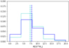Fig. 1. Normalised mass distributions of observed and simulated samples. In cyan we plot the mass distribution in the observed sample. The dashed line represents the median of the distribution at 7.3 × 1014 M⊙. In blue we show the mass distribution in the simulated set. The dashed line represents the median at 7.8 × 1014 M⊙.

In order to increase the sample size, we took three perpendicular projections of each cluster and calculated them as three different clusters. This gave us a total sample size of 216 clusters. It is important to note that the different projections and redshift snapshots of the same clusters are not completely independent. In Appendix B we present arguments that ensure that the overall distribution created in this way does not introduce additional biases due to correlation between the sample constituents.

The redshift ranges and mass distribution of the simulated sample are thus similar to those of the observed sample. This and the above-mentioned proximity of the simulated cluster properties to the properties of observed clusters indicates that the simulated clusters provide a fair representation of the observed set of clusters used in this analysis.

4. Method

In this section we describe the procedure we followed to estimate the value of H₀ using SZ and X-ray observations. This can be subdivided into three stages: i) joint deprojection of the ICM profiles given the SZ and X-ray observables, ii) characterisation of biases of non-cosmological origin, and iii) estimating the value of the Hubble constant.

4.1. Joint deprojection of the ICM profiles

To estimate the 3D electron number density n_e, temperature kT, and pressure P_e profiles, we used the fitting procedure of Bourdin et al. (2017), which we summarise below.

4.1.1. Derivation of n_e(r)

First, X-ray data were used to constrain the 3D n_e(r) profile and to provide an initial approximation of the kT(r) profile. We assumed spherical symmetry and modelled the observable quantities with the analytical profiles suggested by Vikhlinin et al. (2006). More specifically, for the electron number density, we used

$$\begin{array}{cc}& n_p{n}_{\mathrm{e}}(r)=\frac{n_0^2{(r/r_{\mathrm{c}})}^{-{\alpha }^{\prime }}}{{[1+{(r/r_{\mathrm{c}})}^2]}^{3{\beta }_1-{\alpha }^{\prime }/2}}\frac{1}{{[1+{(r/r_{\mathrm{s}})}^{\gamma }]}^{ϵ/\gamma }}\hfill \\ \hfill & +\frac{n_{02}^2}{{[1+{(r/r_{\mathrm{c}2})}^2]}^{3{\beta }_2}},\hfill \end{array}$$(1)

where r_c and r_c2 are the characteristic radii of β-like profiles with slopes β₁ and β₂, with a power-law cusp modification parametrised with the index α′; n₀ and n₀₂ are the normalisations of the two components at the centre; and r_s is the characteristic radius in the outer steeper regions of the profile with slope ϵ.

For the temperature we used

$$\begin{array}{c}\hfill kT(r)=T_0\frac{x+T_{\min }/T_0}{x+1}\frac{{(r/r_t)}^{-a}}{{(1+{(r/r_t)}^b)}^{c/b}},\end{array}$$(2)

where x ≡ (r/r_cool)^a_cool, and r_cool describes the scale of the central cooling region with slope a_cool and normalisation T_min; r_t, a, b, and c describe the size and profile slopes outside the cooling region; and T₀ is the overall normalisation of the profile.

After integrating these 3D models along the line of sight (LOS),

$$\begin{array}{c}\hfill {\mathrm{\Sigma }}_x(r)=\frac{1}{4\pi {(1+z)}^3}{\displaystyle \int [n_{\mathrm{p}}{n}_{\mathrm{e}}]}(r)\mathrm{\Lambda }(T,Z)\mathrm{d}l,\end{array}$$(3)

$$\begin{array}{c}\hfill k{T}_X(r)=\frac{\int wkT(r)\mathrm{d}l}{\int w\mathrm{d}l}\text{, with}\hspace{0.17em}\hspace{0.17em}w=n_{\mathrm{e}}^2/T^{3/4},\end{array}$$(4)

we fit them jointly to the observed projected X-ray surface brightness ${\displaystyle \sum {}_x^{\text{obs}}(r)}$ and temperature $k{T}_X^{\text{obs}}(r)$ profiles obtained from XMM-Newton (see Bourdin et al. 2017 for details).

In Eq. (3) the surface brightness has units cnt s⁻¹ cm⁻² arcmin⁻². If energy units are used, such as erg s⁻¹ cm⁻² arcmin⁻², then the factor 1 + z in the denominator would be to the fourth power, that is, Σ_x(r) = $\frac{1}{4\pi {(1+z)}^4}\int [n_{\mathrm{p}}{n}_{\mathrm{e}}](r)\mathrm{\Lambda }(T,Z)\mathrm{d}l$. In Eq. (4) the temperature weighting from Mazzotta et al. (2004) is used.

Modelling the factor Λ(T, Z) assumes dependence on the metallicity of the gas and weak dependence on temperature. The first was modelled assuming a redshifted, Galactic-hydrogen-absorbed spectral energy distribution (SED) of hot gas with bremsstrahlung continuum and metal emission lines as tabulated in the Astrophysical Plasma Emission Code (APEC, Smith et al. 2001). We adopted the solar composition of metal abundances tabulated by Grevesse & Sauval (1998) and a constant normalisation of 0.3. The fit of the kT(r) in this part of the procedure took care of the weak temperature dependence of the factor Λ(T, Z).

Finally, we derived the electron number density profile $n_{\mathrm{e}}(r)=\sqrt{n_{\mathrm{e}}/n_{\mathrm{p}}\times [n_p{n}_{\mathrm{e}}](r)}$ assuming n_p/n_e = 0.852, which corresponds to a helium abundance of Y = 0.2527 for the metal abundances cited above.

4.1.2. Derivation of P(r) and kT(r)

In the second step, we jointly fit the X-ray projected temperature $k{T}_X^{\text{obs}}(r)$ and SZ y^obs(r) signal profiles. $k{T}_X^{\text{obs}}(r)$ was extracted from the XMM-Newton, while y^obs(r) was extracted from the six Planck HFI maps (see Bourdin et al. 2017 for details).

To model the SZ signal, we used the analytical gNFW pressure profile from Nagai et al. (2007):

$$\begin{array}{c}\hfill P_{\mathrm{e}}(r)=\frac{P_0}{{(c_{500}x)}^{\gamma }{(1+{(c_{500}x)}^{\alpha })}^{(\beta -\gamma )/\alpha }},\end{array}$$(5)

with x ≡ r/r₅₀₀ and r₅₀₀ being defined as the radius of the cluster within which the mean density of the cluster is 500 times higher than the critical density of the Universe at the clusters redshift. P₀ is the overall normalisation of the profile, c₅₀₀ is the concentration with respect to r₅₀₀, and α, β, and γ are the slopes at the inner, intermediate, and outer regions of the profile, respectively.

By fixing the n_e(r) profile to the form obtained in the previous step, we created a template for the temperature as

$$\begin{array}{c}\hfill kT(r)={\eta }_T\times P_{\mathrm{e}}(r)/n_{\mathrm{e}}(r).\end{array}$$(6)

We then integrated Eqs. (5) and (6) along the LOS using

$$\begin{array}{c}\hfill y(r)=\frac{{\sigma }_T}{m_{\mathrm{e}}{c}^2}{\displaystyle \int P_{\mathrm{e}}(r)\times \mathrm{d}l}\end{array}$$(7)

for the pressure profile and Eq. (4) for the temperature, and we fit them jointly to the observed projected y^obs(r) and $T_X^{\text{obs}}(r)$ profiles. In addition to estimating the 3D pressure profile P_e(r), this procedure also returns the value of the normalisation parameter η_T, which reflects the discrepancy between the measurement of pressure profile using only X-ray or SZ observables.

In the ideal case of spherical symmetry with no clumpiness, we expect η_T = 1. In the realistic case, instead, η_T is expected to be different from 1, and its departure depends on different aspects such as the assumptions of the underlying cosmological model and/or some ICM distribution properties (elongation, orientation, clumpiness, etc.).

As shown in Appendix A, η_T has a simple dependence from the main properties that can be divided into two terms:

$$\begin{array}{c}\hfill {\eta }_T=\mathcal{C}\times \mathcal{B}.\end{array}$$(8)

The first term depends only on quantities that are directly related to the cosmological parameters (such as H₀, or Y). It is defined as

$$\begin{array}{c}\hfill \mathcal{C}={\left(\frac{{\overline{D}}_a}{D_a}\right)}^{1/2}\times {\left(\frac{n_{\mathrm{p}}/n_{\mathrm{e}}}{{\overline{n}}_{\mathrm{p}}/{\overline{n}}_{\mathrm{e}}}\right)}^{1/2}\times {\left(\frac{1+4\frac{n_{\mathrm{He}}}{n_{\mathrm{p}}}}{1+4\frac{{\overline{n}}_{\mathrm{He}}}{{\overline{n}}_{\mathrm{p}}}}\right)}^{1/2},\end{array}$$(9)

where D_a is the angular diameter distance, n_p/n_e is the ratio of the hydrogen to electron number density, and $\frac{n_{\mathrm{He}}}{n_{\mathrm{p}}}$ the ratio of helium to hydrogen number density. The latter two factors both depend on the helium abundance Y in the cluster gas (see Appendix A).

The second term contains everything else that is not directly related to the cosmological model or the helium abundance. It can be parametrised as

$$\begin{array}{c}\hfill \mathcal{B}=b_n\frac{C_{\rho }^{1/2}}{e_{\mathrm{LOS}}^{1/2}},\end{array}$$(10)

where e_LOS is a factor that accounts for the cluster asphericity, $C_{\rho }=\frac{⟨{\rho }^2⟩}{{⟨\rho ⟩}^2}$ accounts for the cluster clumpiness, and the factor b_n denotes any other bias that could arise from our profile modelling and/or the fitting procedure.

In the previous two formulas, the non-bar and bar notations of parameters refer to their true values and to the values assumed in the data analysis above, respectively. More specifically, we used a ΛCDM cosmological model with H̄₀ = 70 km s⁻¹ Mpc⁻¹, ${\overline{\mathrm{\Omega }}}_{\mathrm{m}}=0.3$ and ${\overline{\mathrm{\Omega }}}_{\mathrm{\Lambda }}=0.7$, n̄_p/n̄_e = 0.852, and $\frac{{\overline{n}}_{\mathrm{He}}}{{\overline{n}}_{\mathrm{p}}}=0.0851$. For a fully ionised medium, the latter correspond to an assumption of a helium abundance of Ȳ = 0.2527. We refer to Appendix A for a detailed derivation of the Eqs. (8)–(10) above. To constrain the cosmological quantities, we need to characterise the contribution of the ℬ term, which is addressed in the next subsection.

4.2. Characterisation of ℬ

To characterise the ℬ term in Eq. (8), we adopted a simple procedure based on the use of our set of cosmological hydrodynamic simulations that have a clumpiness level comparable to that of real clusters Eckert et al. (2015) and Planelles et al. (2017).

We assumed that the cosmological parameters are known, and we fixed them to the values we used for the simulated sample, that is, a flat ΛCDM cosmology with H₀ = 72 km s⁻¹ Mpc⁻¹ and Ω_m = 0.24, a ratio of hydrogen to electrons n_p/n_e = 0.864, and a number density of helium to hydrogen n_He/n_p = 0.0789 from the fraction of hydrogen mass X = 0.76 (see Sect. 3). These assumptions guarantee that for the simulated sample 𝒞 = 1 (see Eq. (9)). Then, for every simulated cluster, we estimated the parameter η_T applying the exact same procedure used for the real clusters.

In this respect, to imitate the “observed” 2D quantities, we projected the simulated cluster properties by integrating along 10 Mpc in the direction of LOS:

$$\begin{array}{c}\hfill {\mathrm{\Sigma }}_x(r_{\min },r_{\max })=\frac{\sum m_i{\rho }_i}{A_{\mathrm{ring}[r_{\min },r_{\max }]}/\pi },\end{array}$$(11)

$$\begin{array}{c}\hfill T_X(r_{\min },r_{\max })=\frac{\sum T_i{w}_i{V}_i}{\sum T_i{V}_i},\end{array}$$(12)

and

$$\begin{array}{c}\hfill y(r_{\min },r_{\max })=\frac{{\sigma }_T}{m_{\mathrm{e}}{c}^2}\frac{\sum P_i{V}_i}{A_{\mathrm{ring}[r_{\min },r_{\max }]}},\end{array}$$(13)

with the sum extending to all particles within a cylinder of radius [r_min, r_max] and height 10 Mpc; m_i, ρ_i, T_i, P_i, and V_i being the mass, density, temperature, pressure, and the volume of the ith particle, respectively, w_i is the spectroscopic-like weight equal to $w_i={\rho }_i^2/T_i^{3/4}$ (Mazzotta et al. 2004), and $A_{\text{ring}[r_{\text{min}},r_{\text{max}}]}=\pi (r_{\text{max}}^2-r_{\text{min}}^2)$ is the surface area of the cylinders base.

In Fig. 2 we show as a blue histogram the η_T distribution resulting from this procedure. Assuming that the simulated clusters accurately approximate the real ones in terms of i) shape, the gas shape at r₅₀₀ does not strongly depend on the ICM physics and mostly follows the total potential of the cluster (see Lau et al. 2011; Kawahara 2010), and ii) clumpiness level (see Planelles et al. 2017 for comparison), the blue histogram gives the intrinsic distribution of the ℬ term.

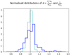Fig. 2. Distribution of the quantity $\frac{1}{e_{\mathrm{LOS}}^{1/2}}$ that was calculated semi-analytically (cyan). Distribution of the quantity $\mathcal{B}\equiv \frac{C_{\rho }^{1/2}}{e_{\mathrm{LOS}}^{1/2}}{b}_n$, which we used as a prior in our Bayesian estimation of the Hubble constant (blue). The dashed line at value 1 is shown for reference.

We expect that asphericity will play a major role. To distinguish its effect from that of clumpiness, we derived the distribution of $e_{\mathrm{LOS}}^{-0.5}$ using the semi-analytical approach of Sereno et al. (2017), which for completeness we also report in Appendix C. The result is overlaid as a cyan histogram in Fig. 2. Comparing the two distributions in Fig. 2, we see that asphericity is indeed important, but it is not the only player, and other terms significantly contribute to the ℬ distribution. The contribution of the remaining components (C_ρ and b_n) in ℬ results in mainly a larger dispersion and a more skewed distribution. Thus, asphericity alone would fail to describe the complete effect of the non-cosmological components, and considering the complete distribution ℬ is crucial to treat them correctly.

4.3. Derivation of the value of H₀

Our approach in this subsection ensures that all contributions in ℬ are considered and are corrected for when deriving cosmological parameters. More precisely, we use the distribution of ℬ as a prior for the non-cosmological bias term in the derivation of H₀ given our data η_T.

The model contains H₀, Y_p, and Ω_m as parameters in common among all clusters (see Eq. (8)). In addition, we have a nuisance parameter ℬ_i for each cluster i. For N data points (sample of N clusters), we have N + 3 parameters in the model. The posterior distribution of H₀ is

$$\begin{array}{cc}& P(H_0)={\displaystyle \int \mathcal{L}(\{{\eta }_T^{(i)}\}|H_0,{\mathrm{\Omega }}_{\mathrm{M}},Y,\{{\mathcal{B}}_i\})\hspace{0.17em}\times \hspace{0.17em}p(\{{\mathcal{B}}_i\})p(H_0)p({\mathrm{\Omega }}_{\mathrm{M}})p(Y)}\hfill \\ \hfill & \times \hspace{0.17em}\mathrm{d}{\mathrm{\Omega }}_{\mathrm{M}}\mathrm{d}Yd{\mathcal{B}}_1\mathrm{d}{\mathcal{B}}_2\dots \mathrm{d}{\mathcal{B}}_N,\hfill \end{array}$$(14)

where we have denoted {ℬ_i} the set of N nuisance parameters ℬ_i. The first factor in the integral is the likelihood. The next four factors in the integral are the prior probabilities of the combined bias terms {ℬ_i} (p({ℬ_i})) and of the parameters H₀, Ω_M, Y – p(H₀), p(Ω_M), and p(Y). We include the parameters Ω_M and Y in this equation, since we would like to include the effect of the uncertainty on these parameters in the final value of H₀.

Assuming uncorrelated cluster measurements, we can write $\mathcal{L}(\{{\eta }_T^{(i)}\left\}\right|H_0$, ${\mathrm{\Omega }}_{\text{M}},\mathcal{Y},\left\{{\mathcal{B}}_i\right\})=\prod \mathcal{L}({\eta }_T^{(i)}|H_0,{\mathrm{\Omega }}_{\text{M}},Y,{\mathcal{B}}_i)$, where now by ℬ_i and ${\eta }_T^{(i)}$ we denote the particular parameter ℬ and measurement η_T for the ith cluster.

Simultaneously, since cluster shapes and clumpiness can be expected not to be correlated, we can also write p({ℬ_i}) = ∏p(ℬ_i).

Then the complete form of the posterior probability of H₀ is

$$\begin{array}{cc}& P(H_0)={\displaystyle \int \prod _i\mathcal{L}({\eta }_T^{(i)}|H_0,{\mathrm{\Omega }}_{\mathrm{M}},Y,{\mathcal{B}}_i)\times \hspace{0.17em}p({\mathcal{B}}_i)p(H_0)p({\mathrm{\Omega }}_{\mathrm{M}})p(Y)}\hfill \\ \hfill & \times \hspace{0.17em}\mathrm{d}{\mathrm{\Omega }}_{\mathrm{M}}\mathrm{d}Y\mathrm{d}{\mathcal{B}}_1\mathrm{d}{\mathcal{B}}_2\dots \mathrm{d}{\mathcal{B}}_N,\hfill \end{array}$$(15)

where the shape of p(ℬ_i) is defined by the distribution derived above. The prior distribution p(H₀) is taken to be uniform between 50 and 100, and null otherwise. The prior distribution p(Ω_M) is also taken to be uniform between 0.25 and 0.35, and null otherwise. Finally, the prior distribution p(Y) is taken to be uniform between 0.24 and 0.25, and null otherwise. The measured distribution of ${\eta }_T^{(i)}$ is shown in Fig. 3.

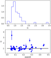Fig. 3. Distribution of values of ηT derived for a sample of 61 clusters using the method described in Sect. 4 (top). The same values as a function of redshift (bottom).

The actual application of the distribution shown in Fig. 2 (limited to the range 0.7 < ℬ_i < 1.65) as a prior distribution of ℬ_i requires extending the distribution over the entire range of values over which the sampling of ℬ_i is done. In order to accomplish this, we approximated the tails of the distribution with a Gaussian distribution (see Appendix D for details and plot). The left side of the distribution is in agreement with a Gaussian tail (see Fig. D.1), hence its extension with a Gaussian can be assumed to describe the real distribution over the ranges 0 < ℬ_i < 0.7 well. The right tail of the distribution is flatter, however, and cannot be described by a Gaussian. This indicates that in the future, a more complete distribution could help to better reconstruct the right tail of p(ℬ_i). We plan to use a larger set of simulated clusters for this in a forthcoming work. For the Markov chain Monte Carlo (MCMC) sampling we used the PyMC python open source MCMC sampler (Fonnesbeck et al. 2015).

5. Results

The procedure described in Sect. 4.1 returns 61 η_T values, one for each observed cluster. In Fig. 3 we show the distribution of these values as well as the same values as a function of redshift. As shown in the previous section, the dispersion of the distribution is due to the intrinsic scatter ℬ shown in Fig. 2 convolved with the measurement error. The main cosmological information comes from the shift relative to p(ℬ) that depends on the true value of H₀.

We applied the procedure described in Sect. 4.3 to constrain H₀ with the observed η_T distribution. We derived the posterior distribution of H₀ in two cases. At first, we ignored the intrinsic non-cosmological biases accounted for in the ℬ parameter. This means that for this test, we assumed spherical symmetry and regularity for galaxy clusters, or in other words, ℬ_i ≡ 1. In Fig. 4 we show the corresponding posterior distribution of H₀ with a dashed line.

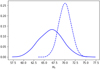Fig. 4. Posterior distributions of H0 for a flat ΛCDM universe. The dashed line is the value of H0 when the bias correction is not applied. The solid line represents the posterior for H0 with the correction for the biases included.

Subsequently, we derived the posterior probability of H₀ by also taking into account the bias terms ℬ_i and assuming the prior p(ℬ_i) obtained from simulations (see Sect. 4.2). The corresponding posterior distribution is overlaid in Fig. 4 as a continuous line.

The comparison of the posterior probabilities in Fig. 4 suggests that the inclusion of p(ℬ_i) leads to i) a broader distribution, and ii) a shift of the mean value. The first arises because we included additional uncertainties. The shift, instead, is caused by the fact that the intrinsic distribution of ℬ is non-symmetrical (see Fig. 2).

We finally report the estimated values within 1σ significance level error: H₀ = 70 ± 1.5 km s⁻¹ Mpc⁻¹, when we ignore the intrinsic biases and H₀ = 67 ± 3 km s⁻¹ Mpc⁻¹, when we correctly account for it.

6. Discussion and conclusions

We introduced a new approach for measuring the value of the Hubble constant using SZ and X-ray observations of clusters of galaxies. The method allows for a simultaneous treatment of the statistical and systematic errors. In this section we compare and discuss our result with previous measurements made using SZ and X-ray observations of clusters as well as other estimations performed with different probes.

6.1. Comparison with other measurements using SZ and X-ray data

In Table 1 we report a non-comprehensive list of measurements of H₀ from SZ and X-ray observations of clusters. In addition to the instruments used for the observations, we also report the sizes of the samples and the corresponding estimates of H₀. These values are all consistent within the statistical plus systematic errors. This may also be due to relatively large total errors (which are at least 14%). For comparison purposes, in Fig. 5 we report the measurement obtained using the two largest cluster samples (i.e. Reese et al. 2004; Bonamente et al. 2006) together with ours. We also add the measurement of Schmidt et al. (2004), which, although they used a sample composed of only three clusters, returns the smallest uncertainty. According to the authors, the use of regular clusters significantly reduces the possible contribution from the systematic errors.

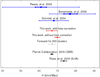Fig. 5. Comparison of the result in this work (in red) with previous measurements using clusters as a probe (in blue) and with current most precise measurements of H0 using other probes (in black). In grey we show our forecast for a future calculation of H0 with the described method and a sample of 200 clusters.

Figure 5 shows that our measurement, being consistent with previous estimates, has a much smaller error. We attribute this improvement to two main factors: i) the improved data quality, and ii) better estimation and treatment of non-cosmological biases. The former has facilitated the necessity and the possibility of addressing the latter at an improved level. Below we further discuss these aspects.

i) Data quality: The data used in the latest estimates by Bonamente et al. (2006) and Reese et al. (2004) are interferometric data at 30 GHz. The authors estimated the absolute flux calibration at 4% level, and this converts into an 8% error in the final H₀ measurement. Planck data, instead, have a multi-frequency coverage (in our case six bands at 100–860 GHz with well-constrained beams) with an error in absolute flux calibration below 0.5% for bands up to 217 GHz (Planck Collaboration IX 2014; Planck Collaboration VIII 2016a). It spatially resolves and maps clusters near r₅₀₀, allowing constraints on cluster pressure profile shapes and dispersion. On the analysis side, the Planck multi-frequency coverage allows an accurate cleaning of foregrounds and backgrounds for the separation of the SZ signal (see Bourdin et al. 2017). All of these factors substantially minimise many uncertainties on the Compton parameter y that were present previously as a result of the limited frequency coverage and impossibility of foreground cleaning (e.g. contamination from point sources, kSZ confusion, and radio halos).

ii) Estimation and treatment of biases: As described before, the currently improved data quality requires a more careful treatment of the biases of non-cosmological origin. In previous works these uncertainties have been estimated independently and were added in quadrature, while we here accounted for correlations between the various sources. The main sources of these uncertainties are the clumpiness of the cluster gas and the departure from spherical shape and from uniform radial thermal distribution (see e.g. Reese et al. 2010; Roettiger et al. 1997; Kawahara et al. 2008; Wang & Fan 2006; Ameglio et al. 2006; Yoshikawa et al. 1998; Molnar et al. 2002). We discuss how these effects were considered in the literature in relation to the outcome of our work.

The estimates of the clumpiness effect in previous works has been controversial. While there is consensus that clumpiness biases the estimate of H₀ high, the size of the effect is still debated. Kawahara et al. (2008) claimed that the effect is of the order of 10%−30%. Based on numerical simulations, Yoshikawa et al. (1998) claimed the effect to be negligible at low redshifts. Reese et al. (2004) and Bonamente et al. (2006) ignored it for the negligible contribution of clumps that could be detected and excluded from the X-ray data (LaRoque et al. 2006). On the other hand, more recent simulations seem to consistently point towards a value close to 1 near the centre, reaching values significantly higher near r₂₀₀ (Nagai & Lau 2011; Roncarelli et al. 2013; Vazza et al. 2013; Battaglia et al. 2015; Planelles et al. 2017). On average, the clumpiness factor is estimated to be < 1.1 within r₅₀₀, which is the radius range relevant for this work. On the observational side, a number of recent works (Morandi et al. 2013; Eckert et al. 2013, 2015) have also started to converge towards similar results.

The assumption of spherical symmetry, instead, may bias the H₀ estimate in both directions depending on the orientation of the cluster. Sulkanen (1999), Grainge et al. (2002), Udomprasert et al. (2004) and Bonamente et al. (2006) estimated a contribution of 15% for a single cluster, while Reese et al. (2000, 2002) and Reese et al. (2004) reported it to be around 20%. Some authors, under the assumption that the scatter introduced by the asphericity of the clusters will average out for a large sample, considered their large set exempt from orientation bias (Bonamente et al. 2006; Kawahara et al. 2008; Sulkanen 1999). However, in Fig. 2 we demonstrate that the contribution from asphericity is not symmetric and could eventually introduce biases. Our treatment of the ℬ factor properly accounts for this potential source of error.

Finally, isothermality of the gas distribution has usually been assumed, leading to an underestimation of H₀ by at least 10% (Reese et al. 2010; Kawahara et al. 2008), even if other studies quantify the error as high as 10–30% (Inagaki et al. 1995; Roettiger et al. 1997).

Many sources of errors that were previously considered as systematics are coherently treated in our statistical Bayesian approach thanks to the informed priors. As shown in Fig. 5, our combined treatment of the uncertainties finally results in a 4% overall error accounting for all the above-mentioned effects and for the uncertainties in the values of Ω_M and Y.

It is important to mention that in this work, which relies on XMM-Newton and Planck observations, we did not account for the cross-calibration issues between XMM-Newton and other X-ray instruments. Instead we assumed that the XMM-Newton observed temperature represents the true temperature of the ICM, while it is known that Chandra returns higher ICM temperatures. Estimates of this temperature discrepancy, however, show a large scatter in the literature (e.g. Snowden et al. 2008; Nevalainen et al. 2010; Martino et al. 2014; Schellenberger et al. 2015). In the current literature it is easy to find temperature discrepancies of anywhere between 0–20% for kT ≈ 6 keV, which corresponds to the median temperature of our sample. This is partly because temperature measurements strongly depend on the choices of the detectors and/or energy bands. A percentile variation in temperature for a single cluster results in a variation of η_T by the same percentile amount in the same direction. Despite this, it is not trivial to estimate the total effect on H₀ due to the entire sample because i) the sample has a temperature distribution and the discrepancy depends on the actual cluster temperature; ii) in our analysis we probe external regions (≈r₅₀₀) of the cluster, where the cluster temperatures drop. This will likely reduce the overall effect. It is beyond the scope of this paper to address this specific issue in detail, and we leave its investigation for future work.

6.2. Comparison with other cosmological probes

In this subsection we discuss the comparison of our result with derivations of the value of H₀ using other cosmological probes. As described in the introduction, we cannot easily attribute the discrepancy between the high-redshift CMB estimate (H₀ = 66.93 ± 0.62 km s⁻¹ Mpc⁻¹ Planck Collaboration Int. XLVI 2016) and the low-redshift estimate using SNIa (H₀ = 73.48 ± 1.66 km s⁻¹ Mpc⁻¹ Riess et al. 2018a or H₀ = 73.52 ± 1.62 km s⁻¹ Mpc⁻¹ from Riess et al. 2018b) to a specific systematic in one particular measurement. In particular, alternative measurements that avoid the use of one or the other data set are either so far unable to reach the given precisions or also encounter similar inconsistencies (Riess et al. 2018a; Bernal et al. 2016). For example, the measurement using time delays of strongly lensed images of three quasars by the H0LiCOW project (Bonvin et al. 2017) leads to a completely independent measurement of $H_0=71.9_{-3.0}^{+2.4}$ km s⁻¹ Mpc⁻¹ for a flat ΛCDM with H₀ and Ω_Λ left free. When allowing only H₀ to vary, the result is instead H₀ = 72.8 ± 2.4 km s⁻¹ Mpc⁻¹. Through geometric distance measurements to the megamaser galaxy NGC 5765b, Gao et al. (2016) determined H₀ = 66.0 ± 6.0 km s⁻¹ Mpc⁻¹. Other probes based on the baryon acoustic oscillations (BAO) combined with data independent of CMB and SNIa provide $H_0=67.2_{-1.0}^{+1.2}$ km s⁻¹ Mpc⁻¹ by Abbott et al. (2018; BAO and Dark Energy Survey Year 1 clustering and weak-lensing data combined with Big Bang nucleosynthesis information), H₀ = 66.98 ± 1.18 km s⁻¹ Mpc⁻¹ from Addison et al. (2018; BAO from galaxy and Lyα forest with an estimate of primordial deuterium abundance). At the same time, BAO in combination with other CMB measurements from the Wilkinson Microwave Anisotropy Probe (WMAP), the South-Pole Telescope (SPT), the Atacama Cosmology Telescope (ACT), and SNIa data provide H₀ = 69.6 ± 0.7 km s⁻¹ Mpc⁻¹ from Bennett et al. (2014) or in combination with observational Hubble datasets and SNIa data H₀ = 69.4 ± 1.7 km s⁻¹ Mpc⁻¹ from Haridasu et al. (2018).

In the light of the possible cosmological solutions suggested so far (Riess et al. 2016; Bernal et al. 2016; Evslin & Sen 2018; Lin & Ishak 2017) that tried to resolve the discrepancy between the CMB and local measurements of H₀, we briefly discuss the importance of these scenarios for our measurement, which is perfectly consistent with the result of Planck Collaboration Int. XLVI (2016) and is compatible within 2σ with Riess et al. (2018a). The current possible cosmological extensions aim to decrease the discrepancy between the CMB measurement and low-redshift SNIa measurements by either modifying early-Universe physics (e.g. BBN, density of relativistic species) in order to increase the CMB result or by changing the late-time evolution of the Universe in order to introduce recent evolution in the value of H₀ allowing for the difference between the early- and late-time measurements. Given that our result is based on low-redshift data, and it is in the lower range of values, modifications of late-time evolution aiming to bring to an increase in the value of H₀ in the local Universe are not required by our findings. The possible modifications in early-time evolution would modify the CMB measurement by moving it towards higher values. In particular, any changes in the value of Y (the only relevant quantity in this work) that were required to reconcile the CMB H₀ constraints with the SNIa would lower our measurement of H₀.

Thus, being a method that does not rely on additional distance ladders, the use of galaxy clusters to determine a local value of the Hubble constant could be decisive in solving this issue in the future. However, more stringent constraints are required for solid conclusions.

6.3. Estimating possible improvements to accuracy

An improvement to the current result could be achieved by applying this method to larger samples. To estimate the accuracy that could be reached, we created a toy model with “measurements” of η_T distributed as our sample (with the same mean and scatter). To these data points we assigned errors equal to the average error on η_T in our data. We then repeated the procedure to fit the value of H₀ for various sizes of our toy sample. In Fig. 6 we report our estimated error size for various sample sizes. We found the final error to vary roughly as the square root of the number of clusters ($\frac{1}{\sqrt{N}}$), as demonstrated in the figure with the overlaid line corresponding to 3.0 × ${\left(\frac{60}{N}\right)}^{1/2}$. It is remarkable how a future application of this technique to a sample of 200 clusters would narrow down the error on H₀ to a 3% level, as is also shown by the point added to Fig. 5. High-quality Chandra and XMM-Newton follow-up observations of the Planck cluster catalogue are ongoing and are expected provide us with such constraints in the near future.

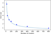Fig. 6. Prediction of the error depending on the sample size (blue triangles) over-plotted with the function $3.0\times {\left(\frac{60}{N}\right)}^{1/2}$ (dashed line).

Acknowledgments

We thank Alex Saro and Balakrishna Sandeep Haridasu for useful discussions, and we acknowledge financial contribution from the agreement ASI-INAF n.2017-14-H.O, from ASI Grant 2016-24-H.0., and from “Tor Vergata” Grant “Mission: Sustainability” EnClOS (E81I18000130005).

References

Appendix A: Dependence of η_T on cluster and cosmological parameters

In this appendix we derive the analytic form of the dependence of η_T on the parameters describing the cosmological model and the cluster. We have in total three observable quantities that are projected quantities along the LOS that we list below.

• 1)

  The SZ signal is proportional to the integral of the pressure of ICM electrons along the LOS. For a given projected distance r on the plane of the sky (POS) from the cluster centre, the signal is

  $$\begin{array}{c}\hfill y(r)=\frac{{\sigma }_T}{m_{\mathrm{e}}{c}^2}{\displaystyle {\int }_{l=-\infty }^{\infty }{P}_{\mathrm{e}}(l(r))\times \mathrm{d}l,}\end{array}$$(A.1)

  with σ_T, m_e, and P(l) being the Thomson scattering cross-section, the mass of electron, and the pressure of electrons in the ICM, respectively, and l being the physical distance along the LOS (see Fig. A.1).

• 2)

  The X-ray surface brightness is proportional to the integral of the square of the number density of electrons along the LOS:

  $$\begin{array}{c}\hfill S_X(r)=\frac{1}{4\pi {(1+z)}^3}{\displaystyle {\int }_{l=-\infty }^{\infty }[n_{\mathrm{p}}{n}_{\mathrm{e}}](l(r))\mathrm{\Lambda }(T,\xi ,Y)\times \mathrm{d}l,}\end{array}$$(A.2)

  where z is the cluster redshift, n_p and n_e are the number density of protons (i.e. hydrogen, denoted also as n_H in literature) and electrons in the ICM. The factor Λ(T, ξ, Y) is the cooling function that depends on the temperature, the abundance of helium (represented here with Y), and abundances of other elements heavier than helium in the cluster gas (ξ). This function combines the emission due to all the elements responsible for the X-ray continuum emission, mainly hydrogen and helium. We also note that here the surface brightness has units cnt s⁻¹ cm⁻² arcmin⁻². If energy units are used, such as erg s⁻¹ cm⁻² arcmin⁻², then the factor 1 + z in the denominator would be to the fourth power, that is, ${\mathrm{\Sigma }}_x(r)=\frac{1}{4\pi {(1+z)}^4}\int [n_{\mathrm{p}}{n}_{\mathrm{e}}](r)\mathrm{\Lambda }(T,Z)\mathrm{d}l$. We converted $n_{\mathrm{p}}{n}_{\mathrm{e}}=\frac{n_{\mathrm{p}}}{n_{\mathrm{e}}}\times n_{\mathrm{e}}^2$, leaving n_e(l(r))² as a profile to be modelled and $\frac{n_{\mathrm{p}}}{n_{\mathrm{e}}}$ a factor that is fixed by the abundance of other elements in the gas relative to hydrogen. At the end of this appendix, we show how this factor is related to the element abundances in the gas. On the other hand, the factor Λ(T, ξ, Y) can be expressed as the sum of contributions from hydrogen and helium separately, namely Λ(T, ξ, Y)=Λ_H(T) × $(1+4\frac{n_{\mathrm{He}}}{n_{\mathrm{p}}})$, where Λ_H(T) denotes the contribution only from hydrogen and the factor $4\frac{n_{\mathrm{He}}}{n_{\mathrm{p}}}$ adds to this the contribution from helium only (assuming all the other elements contribute negligibly to the X-ray continuum). Thus the final form of the X-ray surface brightness is the following:

  $$\begin{array}{c}\hfill S_X(r)=\frac{1}{4\pi {(1+z)}^3}\times \frac{n_{\mathrm{p}}}{n_{\mathrm{e}}}(1+4\frac{n_{\mathrm{He}}}{n_{\mathrm{p}}})\times {\displaystyle {\int }_{l=-\infty }^{\infty }{n}_{\mathrm{e}}{(l(r))}^2{\mathrm{\Lambda }}_{\mathrm{H}}(T)\times \mathrm{d}l,}\end{array}$$(A.3)

• 3)

  The projected temperature, which we approximate with the spectroscopic-like temperature of Mazzotta et al. (2004):

  $$\begin{array}{c}\hfill k{T}_X(r)=\frac{{\int }_{l=-\infty }^{\infty }W(l(r))kT(l(r))\times \mathrm{d}l}{{\int }_{l=-\infty }^{\infty }W(l(r))\times \mathrm{d}l},\end{array}$$(A.4)

  where $W(l)=\frac{n_{\mathrm{e}}{(l)}^2}{kT{(l)}^{3/4}}$, k is the Boltzman constant and T is the temperature of the cluster gas.

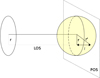Fig. A.1. Schematic of the signal projection and the definitions used in Appendix A. POS and LOS denote the POS and the LOS direction. r is the projected distance from the cluster centre, r′ the 3D spherical distance from cluster centre, and l the distance in the direction of LOS from the cluster centre. Given these definitions, we can write r′2 = r2 + l2.

Next we write the previous equations in function of the projected POS distance from the cluster centre r, using the relation r′² = r² + l², where r′ is the 3D spherical distance from the cluster centre. We also convert the quantities representing physical distance to quantities defined relative the characteristic scale of the cluster $x=\frac{r}{r_{500}}$. For the three observables, this conversion would result in the following forms:

$$\begin{array}{c}\hfill y(\theta )=P_0{e}_{\mathrm{LOS}}\times D_A{\theta }_{500}\times f_{\mathrm{SZ}},\end{array}$$(A.5)

$$\begin{array}{c}\hfill S_X(\theta )=\frac{1}{4\pi {(1+z)}^3}\times \frac{n_{\mathrm{p}}}{n_{\mathrm{e}}}(1+4\frac{n_{\mathrm{He}}}{n_{\mathrm{p}}})\times n_{\mathrm{e}0}^2{C}_{\rho }{e}_{\mathrm{LOS}}\times D_A{\theta }_{500}\times f_X,\end{array}$$(A.6)

$$\begin{array}{c}\hfill T_X(\theta )=k{T}_0\times f_T,\end{array}$$(A.7)

where in order to simplify the form of the equations, we have defined the factors

$$\begin{array}{cc}\hfill f_{\mathrm{SZ}}& \equiv 2{\displaystyle {\int }_{x^{\prime }=x}^{X_{\max }}\frac{(P(x^{\prime })/P_0)x^{\prime }}{\sqrt{x^{{\prime }^2}-x^2}}}\times \mathrm{d}{x}^{\prime },\hfill \\ \hfill f_X& \equiv 2{\displaystyle {\int }_{x^{\prime }=x}^{X_{\max }}\frac{(n_{\mathrm{e}}^2(x^{\prime })/n_{\mathrm{e}0}^2){\mathrm{\Lambda }}_{\mathrm{H}}{x}^{\prime }}{\sqrt{x^{{\prime }^2}-x^2}}}\times \mathrm{d}{x}^{\prime },\hfill \\ \hfill f_T& \equiv \frac{{\int }_{x^{\prime }=x}^{X_{\max }}\frac{W(x^{\prime })kT(x^{\prime })/k{T}_0{x}^{\prime }}{\sqrt{x^{{\prime }^2}-x^2}}\times \mathrm{d}{x}^{\prime }}{{\int }_{x^{\prime }=x}^{X_{\max }}\frac{W(x^{\prime })x^{\prime }}{\sqrt{x^{{\prime }^2}-x^2}}\times \mathrm{d}{x}^{\prime }},\hfill \end{array}$$

and taken out the normalisations of all quantities P_e, n_e, and T. We also express r₅₀₀ in terms of the observable quantity ${\theta }_{500}=\frac{r_{500}}{D_A}$, where D_A is the angular diameter distance to the cluster. The factor e_LOS is introduced in all the integrals as a correction for the approximation of spherical symmetry. In the simplest case of an elliptical cluster aligned with any of its axes along the LOS, this quantity could be written as $e_{\mathrm{LOS}}=\frac{r_{\Vert }}{r_{\perp }}$, where r_∥ and r_⊥ are the size of the cluster in the LOS direction and in the POS, respectively. In more complicated cases of random orientation and more complicated shape of the cluster, this factor has a complex dependence on those quantities and can be treated as a general correction term for asphericity. Finally, the factor $C_{\rho }\equiv \frac{⟨{\rho }^2⟩}{{⟨\rho ⟩}^2}$ is introduced as a correction taking care of the clumpiness of the cluster gas. The clumpiness results in enhanced X-ray emission, so that C_ρ by definition is always larger than 1.

Equations (A.5)–(A.7) exhibit the explicit dependence of the observables on the normalisations of the cluster properties such as P_e, n_e, and T, the cosmological model, and the deviations of the cluster gas from our assumptions. We next try to relate them to the parameter η_T as derived in Sect. 4.

In order to do this, we distinguish a case 1) in which the true cosmological model and parameters as well as the cluster characteristics are known from a case 2) that corresponds to our modelling described in Sect. 4, which does not necessarily have to be the true model of the Universe and the cluster: a ΛCDM cosmological model with H̄₀ = 70 km s⁻¹ Mpc⁻¹, ${\overline{\mathrm{\Omega }}}_m=0.3,$ and ${\overline{\mathrm{\Omega }}}_{\mathrm{\Lambda }}=0.7$ and spherical clusters without clumps. Hereafter we use the bar notation to distinguish the parameters for which a value potentially different from truth has been assumed.

Our fitting procedure returns η_T that in essence reflects the discrepancy of the normalisation of profiles measured with X-ray and SZ observables. Then for case 1), Eqs. (A.5)–(A.7) can be combined in the following way:

$$\begin{array}{cc}& \frac{k{T}_0}{P_0/n_{\mathrm{e}0}}={\langle \frac{f_{\mathrm{SZ}}}{y(\theta )}\rangle }_{\theta }\times {\langle \frac{k{T}_X(\theta )}{f_T}\rangle }_{\theta }\times {\langle \sqrt{\frac{S_X(\theta )}{f_X}}\rangle }_{\theta }\hfill \\ \hfill & \times \hspace{0.17em}{\left(\frac{1}{n_{\mathrm{p}}/n_{\mathrm{e}}}\right)}^{1/2}{\left(\frac{1}{1+4\frac{n_{\mathrm{He}}}{n_{\mathrm{p}}}}\right)}^{1/2}\times \hspace{0.17em}{\left(\frac{e_{\mathrm{LOS}}}{C_{\rho }}\right)}^{1/2}\hfill \\ \hfill & \times \hspace{0.17em}{\theta }_{500}^{1/2}{D}_a^{1/2}{(1+z)}^{3/2}\equiv 1,\hfill \end{array}$$(A.8)

where we denote with the brackets <>_θ the fact that the fitted normalisation values carry averaged information from the observed profiles. The equivalence on the right comes from the relation P₀ ≡ n_e0 × kT₀.

For case 2), the equivalence is instead not true, since our assumptions bias the measured values of P₀, n_e0, and T₀:

$$\begin{array}{cc}& {\eta }_T\equiv \frac{k{\overline{T}}_0}{{\overline{P}}_0/{\overline{n}}_{\mathrm{e}0}}={\langle \frac{f_{\mathrm{SZ}}}{y(\theta )}\rangle }_{\theta }\times {\langle \frac{k{T}_X(\theta )}{f_T}\rangle }_{\theta }\times {\langle \sqrt{\frac{S_X(\theta )}{f_X}}\rangle }_{\theta }\hfill \\ \hfill & \times {\left(\frac{1}{{\overline{n}}_{\mathrm{p}}/{\overline{n}}_{\mathrm{e}}}\right)}^{1/2}{\left(\frac{1}{1+4\frac{{\overline{n}}_{\mathrm{He}}}{{\overline{n}}_{\mathrm{p}}}}\right)}^{1/2}\times {\left(\frac{{\overline{e}}_{\mathrm{LOS}}}{{\overline{C}}_{\rho }}\right)}^{1/2}\hfill \\ \hfill & \times {\overline{\theta }}_{500}^{1/2}{\overline{D}}_a^{1/2}{(1+z)}^{3/2}\ne 1.\hfill \end{array}$$(A.9)

In this case, the contribution from ${\overline{C}}_{\rho }$ and ē_LOS has been ignored in our fitting procedure described in Sect. 4, so that these quantities have been considered equal to 1 $({\left(\frac{{\overline{e}}_{\mathrm{LOS}}}{{\overline{C}}_{\rho }}\right)}^{1/2}=1)$.

Removing the factor ${\left(\frac{{\overline{C}}_{\rho }}{{\overline{e}}_{\mathrm{LOS}}}\right)}^{1/2}$ and taking the ratio of Eqs. (A.8) and (A.9) brings us to an expression for the ratio ${\eta }_T\equiv \frac{k{\overline{T}}_0}{{\overline{P}}_0/{\overline{n}}_{\mathrm{e}0}}$ measured in our fitting procedure,

$$\begin{array}{cc}& {\eta }_T\equiv b_n\frac{k{\overline{T}}_0}{{\overline{P}}_0/{\overline{n}}_{\mathrm{e}0}}=b_n{\left(\frac{C_{\rho }}{e_{\mathrm{LOS}}}\right)}^{1/2}\times {\left(\frac{{\overline{\theta }}_{500}{\overline{D}}_a}{{\theta }_{500}{D}_a}\right)}^{1/2}\hfill \\ \hfill & \times {\left(\frac{n_{\mathrm{p}}/n_{\mathrm{e}}}{{\overline{n}}_{\mathrm{p}}/{\overline{n}}_{\mathrm{e}}}\right)}^{1/2}\times {\left(\frac{1+4\frac{n_{\mathrm{He}}}{n_{\mathrm{p}}}}{1+4\frac{{\overline{n}}_{\mathrm{He}}}{{\overline{n}}_{\mathrm{p}}}}\right)}^{1/2},\hfill \end{array}$$(A.10)

where as a final step we introduced a factor b_n that represents any other biases that are contained in our fitting procedure that have not yet been included in the equations.

At this point, we simplify the two factors $\left(\frac{{\overline{\theta }}_{500}{\overline{D}}_a}{{\theta }_{500}{D}_a}\right)$ and ${\left(\frac{n_{\mathrm{p}}/n_{\mathrm{e}}}{{\overline{n}}_{\mathrm{p}}/{\overline{n}}_{\mathrm{e}}}\right)}^{1/2}\times {\left(\frac{1+4\frac{n_{\mathrm{He}}}{n_{\mathrm{p}}}}{1+4\frac{{\overline{n}}_{\mathrm{He}}}{{\overline{n}}_{\mathrm{p}}}}\right)}^{1/2}$ in the following way:

1. θ₅₀₀ vs ${\overline{\theta }}_{500}$: θ₅₀₀ is an observable quantity, which means that θ₅₀₀, which the cluster appears to have given the true cosmological model and the cluster distance and size, should be equal to the ${\overline{\theta }}_{500}$ that we observe.

2. Conversion of $\frac{n_{\mathrm{He}}}{n_{\mathrm{p}}}$ and n_p/n_e to Y (mass ratio of helium to hydrogen) dependent factors: We introduce the definitions of abundance in terms of number density and mass. We denote the abundance in terms of number density of a given element relative to hydrogen as n_i/n_p (equivalent to n_i/n_H). The abundance in terms of mass, instead, is denoted as m_i/m_H = A_in_i/(A_Hn_p) = A_in_i/n_p, where A_i is the atomic number of a given element. In our calculations we make use of measurements of element abundances in cluster gas in terms of number density reported by Grevesse & Sauval (1998) normalised by a constant 0.3. Thus we have the values of n_i/n_p for elements up to i = 26. Having the n_i/n_p and the atomic number A_i of each element, the ratio n_p/n_e can be expressed in the following way:

   $$\begin{array}{c}\hfill \frac{n_{\mathrm{p}}}{n_{\mathrm{e}}}=\frac{1}{1+\frac{n_{\mathrm{He}}}{n_{\mathrm{p}}}{A}_{\mathrm{He}}+{\sum }_{i=3}^{26}\frac{n_i}{n_{\mathrm{p}}}{A}_i}={(1+2\frac{n_{\mathrm{He}}}{n_{\mathrm{p}}}+\xi )}^{-1},\end{array}$$(A.11)

   where we introduce the notation $\xi \equiv \sum _{i=3}^{26}\frac{n_i}{n_{\mathrm{p}}}{A}_i$. Given the metallicity and the abundances we use, this quantity is fixed to ξ = 3.46 × 10⁻³. At the same time, the mass ratio of helium to hydrogen is

   $$\begin{array}{c}\hfill Y=\frac{m_{\mathrm{He}}}{m_{\mathrm{H}}}=\frac{2\frac{n_{\mathrm{He}}}{n_{\mathrm{p}}}{A}_{\mathrm{He}}}{1+2\frac{n_{\mathrm{He}}}{n_{\mathrm{p}}}{A}_{\mathrm{He}}+{\sum }_{i=3}^{26}2\frac{n_i}{n_{\mathrm{p}}}{A}_i}=\frac{4\frac{n_{\mathrm{He}}}{n_{\mathrm{p}}}}{1+4\frac{n_{\mathrm{He}}}{n_{\mathrm{p}}}+2\xi }·\end{array}$$(A.12)

   Expressing $\frac{n_{\mathrm{He}}}{n_{\mathrm{p}}}$ in terms of Y and substituting in the expression of n_p/n_e, we obtain

   $$\begin{array}{c}\hfill {\left(\frac{n_{\mathrm{p}}}{n_{\mathrm{e}}}\right)}^{1/2}\times {(1+4\frac{n_{\mathrm{He}}}{n_{\mathrm{p}}})}^{1/2}={\left(\frac{2+4Y\xi }{2-Y+2\xi }\right)}^{1/2}.\end{array}$$(A.13)

   Substituting the values of n̄_p/n̄_e = 0.852 and $\frac{{\overline{n}}_{\mathrm{He}}}{{\overline{n}}_{\mathrm{p}}}=0.0851$ corresponding to the helium abundance assumed in our analysis:

   $$\begin{array}{c}\hfill {\left(\frac{n_{\mathrm{p}}/n_{\mathrm{e}}}{{\overline{n}}_{\mathrm{p}}/{\overline{n}}_{\mathrm{e}}}\right)}^{1/2}\times {\left(\frac{1+4\frac{n_{\mathrm{He}}}{n_{\mathrm{p}}}}{1+4\frac{{\overline{n}}_{\mathrm{He}}}{{\overline{n}}_{\mathrm{p}}}}\right)}^{1/2}={\left(\frac{2+4Y\xi }{2-Y+2\xi }\right)}^{1/2}\times {\left(\frac{1}{0.852\times 0.0851}\right)}^{1/2}.\end{array}$$(A.14)

The complete form for η_T is then the following:

$$\begin{array}{c}\hfill {\eta }_T=b_n{\left(\frac{C_{\rho }}{e_{\mathrm{LOS}}}\right)}^{1/2}\times {\left(\frac{{\overline{D}}_a}{D_a}\right)}^{1/2}\times {\left(\frac{2+4Y\xi }{1.142\times (2-Y+2\xi )}\right)}^{1/2}.\end{array}$$(A.15)

Appendix B: Treating the correlations within the simulated sample

Following the procedure of Rasia et al. (2013), we checked whether using a set of not fully independent realisations of the same simulated clusters biases our results. We have 26 objects in total, each with three projections at two or three different redshifts: some at z = 0.25 and z = 0.5 have masses below our mass cut. This amounts to a total of 216 realisations. We generated 1000 subsamples of 26 independent realisations by randomly sampling one from the available realisations of each of the 26 objects. We checked through the K–S test the compatibility of the η⁽²⁶⁾ distribution of each of the sub-samples with the overall η_T distribution (shown in Fig. 2). We obtained the K–S distribution for the 1000 sub-samples shown in Fig. B.1. In only 2% of the sub-samples can the similarity hypothesis between the distributions (that derived from one sub-sample and the overall distribution) be rejected with a confidence level at least equal to 0.05 (vertical dashed line in the figure).

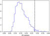Fig. B.1. Distribution of the Kolmogorov–Smirnov statistic value when comparing the distribution of ηT in Fig. 4.2 and the 1000 realisations of the ${\eta }_T^{(26)}$ distribution for independent cluster sub-sets of the total 216 cluster set. The dashed line represents the value for which the similarity of the given sub-distribution of ${\eta }_T^{(26)}$ and the entire distribution ηT can be rejected at 0.05 confidence. These cases constitute only 2% of all.

The figure shows that our final distribution of η_T probably does not carry amplified biases that are due to the dependence of the object realisations in the sample. This agrees with the majority of the possible subsets of independent realisations.

Appendix C: Semi-analytical estimation of bias that is only due to asphericity

Here we give the details of the procedure of deriving a distribution of $\frac{1}{e_{\mathrm{LOS}}^{1/2}}$ in a sample similar to our sample of Planck clusters. It can be divided into two main steps: i) given the distribution of SZ mass and redshift of our Planck sample, we derive the corresponding virial mass-redshift distribution from it, and ii) given the virial masses of the clusters, we randomly assign them an elliptical shape in agreement with their mass and an orientation relative to the LOS. We finally project the cluster with given shape and orientation in order to calculate the projection ratio $e_{\mathrm{LOS}}=\frac{r_{\Vert }}{r_{\perp }}$, with r_∥ being the size of the cluster along our LOS and r_⊥ being its projected size on the POS.

C.1. Derivation of [M_v, z] given [M_SZ, z]

• [M_SZ, z]. We start our calculation starting from the SZ mass-redshift distribution of the Planck sample of clusters that we used in this paper.

• Derivation of [M₅₀₀, z]. Taking an approximate value of the SZ bias for Planck clusters as b_SZ = 0.25 (see Planck Collaboration XXIV 2016; Sereno et al. 2017), we derive M₅₀₀ = (1 + b_SZ)M_SZ.

• Derivation of [M₂₀₀, c₂₀₀, z]². Hu & Kravtsov (2003) provide a formula for conversions between definitions of halo mass under the assumption of a Navarro-Frenk-White (NFW) density profile. Thus given a set [M_Δx, c_Δx, Δ_x], where M_Δx and c_Δx are the known mass and concentration parameter at a given mass overdensity Δ_x, they provide a formula to derive a set of [M_Δy, c_Δy] at overdensity Δ_y. At the same time, Meneghetti et al. (2014) provide a formula to relate c₂₀₀ to M₂₀₀ in the following form: $c_{200}(M_{200},z)=A\times {\left(\frac{1.35}{1+z}\right)}^B\times {\left(\frac{M_{200}}{8\times {10}^{14}{\mathrm{h}}^{-1}{M}_{\odot }}\right)}^C$, where the values of parameters A, B and C are fit assuming a NFW density profile using the MUSIC 2 hydrodynamic simulated massive clusters. The relationship also includes an intrinsic scatter. Using these conversions and the scatter in agreement with Meneghetti et al. (2014), we can establish the pair [M₂₀₀, c₂₀₀ = c₂₀₀(M₂₀₀, z)] that corresponds to each pair of [M₅₀₀, z] in our set.

• Derivation of Δ_v ³ and [M_v, z]. Bryan & Norman (1998) derived an approximate scaling formulae for a number of virial quantities for a range of redshifts in three different cosmological models. In particular, they fit a formula for the overdensity at virial radius relative to the critical density of the Universe given the redshift and the cosmological model. Converting their formula to derive the overdensity relative to the mean matter density, we derive a value of Δ_v for the redshift of each cluster. Then given [M₂₀₀, c₂₀₀, Δ₂₀₀, Δ_v] again referring to Hu & Kravtsov (2003), we derive a value of M_v for each cluster in our set.

At the end of this first part, we then have the distribution of [M_v, z] of our Planck sample of clusters. We can now create a large representation of this distribution. We pull out N = 30 000 realisations of M_v from this distribution.

C.2. Derivation of the asphericity ratio distribution given M_v

In this part we use the N values of the virial mass and chose random shapes and orientations in agreement with these masses in order to calculate the projection ratio e_LOS for these N clusters. We later assume that this represents the distribution of e_LOS of our set of clusters.

• DM axis ratios. Using Millennium XXL simulations, Bonamigo et al. (2015) derived simple functional forms for axis ratio distributions of clusters with given virial mass. These formulae take as input the cluster virial mass and output a probability distribution function for the minor-to-major and intermediate-to-major axis ratios. Given the N masses of clusters of our set, we chose N random values for the axis ratios following these distributions.

• ICM axis ratios. Kawahara (2010) constructed a model that allows deriving the axis ratio of the gas distribution in the cluster based on the DM distribution and the assumption of hydrostatic equilibrium (HE). This is done based on the argument that the matter distribution follows the DM isopotentials due to HE. Following Kawahara (2010), we calculate the isopotential surfaces for a given DM distribution. Considering the cluster gas to follow the isopotentials, we take the ratio of axes of these surfaces as axis ratios of the gas distribution.

• Random orientation with respect to the LOS. We chose random orientations for the N clusters using the three Euler angles.

• Projection of the constructed ICM ellipsoid to derive $e_{\mathrm{LOS}}=\frac{r_{\Vert }}{r_{\perp }}$ and consequently $\frac{1}{e_{\mathrm{LOS}}^{1/2}}$. Sereno et al. (2017) provided formulae for projecting a triaxial ellipsoid with a given orientation defined by the three Euler angles. The eventual derived quantity is the ratio of the LOS length of the cluster and the size of the cluster projection in the POS – $e_{\mathrm{LOS}}=\frac{r_{\Vert }}{r_{\perp }}$. We project the constructed ellipsoid in the POS and the LOS following Sereno et al. (2017). As a measure for r_⊥, we take the geometrical average of the two axes of the cluster projection on the POS. The exact equations for calculating these quantities are given in Sereno et al. (2017).

In conclusion, we use our distribution [M_SZ, z] in order to derive a distribution of $\frac{1}{e_{\mathrm{LOS}}^{1/2}}$. The final distribution is shown in Fig. 2.

Appendix D: Implementing a tabulated distribution as a prior

In this section we describe the extrapolation of the distribution of ℬ derived in Sect. 4.2 over the range explored during the sampling. In Fig. D.1 we show the form of the probability and the cumulative distributions we derived. The values corresponding to each bin are shown with stars. Given our set of 216 clusters, this distribution is defined only over the range 0.7 < ℬ < 1.65. We need to extrapolate it to a wider range of values in order to use it as our prior p(ℬ).

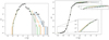Fig. D.1. Extended probability (left) and cumulative (right) distribution functions of ℬ using 1, 3, 5, and 7 counts for the extension shown as black, blue, orange, and green lines, respectively. The actual points of the distribution resulting from the 216 values derived using simulations are shown with stars.

In order to do this, we chose the next to last bins from the tails of the distribution and extended the distribution starting from these points assuming a Gaussian (black line in the figures). In the probability distribution function on the left, we basically ignored the last bins of the histogram tail and extended the area spanned by these bins under a Gaussian shape.

We achieved this by means of the cumulative distribution function (CDF), since the CDF naturally takes care of the normalisation of the final distribution. We cut the CDF at given bins and extended from that point on with a Gaussian CDF with a mean equal to 1.03 (as for our distribution) and with a standard deviation such that the Gaussian CDF passes exactly through the required bin value. The final CDF was then composed of the analytic tails approximated by us and of the tabulated central part that is the direct result of the simulations.

We note that the left side of the resulting distribution agrees well with a Gaussian continuation. The right side, however, seems to be flatter. In order to check the validity of our extrapolation, we repeated the same exercise, but started the extrapolation from bins farther away from the tails, ignoring enough bins to skip 3, 5, or 7 counts from the tails. The curves shown for these extrapolations (blue, orange, and green, respectively) prove once again that the approximation for the Gaussian is good enough for the left side of the distribution, but not for the right side. Despite this small disagreement, we note that the estimated value of H₀ is well within the errors for the extrapolations that do not completely remove the flatness of the right tail (using the one- and three-point approach).

All Tables

All Figures

	Fig. 1. Normalised mass distributions of observed and simulated samples. In cyan we plot the mass distribution in the observed sample. The dashed line represents the median of the distribution at 7.3 × 1014 M⊙. In blue we show the mass distribution in the simulated set. The dashed line represents the median at 7.8 × 1014 M⊙.
In the text

	Fig. 2. Distribution of the quantity $\frac{1}{e_{\mathrm{LOS}}^{1/2}}$ that was calculated semi-analytically (cyan). Distribution of the quantity $\mathcal{B}\equiv \frac{C_{\rho }^{1/2}}{e_{\mathrm{LOS}}^{1/2}}{b}_n$, which we used as a prior in our Bayesian estimation of the Hubble constant (blue). The dashed line at value 1 is shown for reference.
In the text

	Fig. 3. Distribution of values of ηT derived for a sample of 61 clusters using the method described in Sect. 4 (top). The same values as a function of redshift (bottom).
In the text

	Fig. 4. Posterior distributions of H0 for a flat ΛCDM universe. The dashed line is the value of H0 when the bias correction is not applied. The solid line represents the posterior for H0 with the correction for the biases included.
In the text

	Fig. 5. Comparison of the result in this work (in red) with previous measurements using clusters as a probe (in blue) and with current most precise measurements of H0 using other probes (in black). In grey we show our forecast for a future calculation of H0 with the described method and a sample of 200 clusters.
In the text

	Fig. 6. Prediction of the error depending on the sample size (blue triangles) over-plotted with the function $3.0\times {\left(\frac{60}{N}\right)}^{1/2}$ (dashed line).
In the text

	Fig. A.1. Schematic of the signal projection and the definitions used in Appendix A. POS and LOS denote the POS and the LOS direction. r is the projected distance from the cluster centre, r′ the 3D spherical distance from cluster centre, and l the distance in the direction of LOS from the cluster centre. Given these definitions, we can write r′2 = r2 + l2.
In the text

Fig. B.1. Distribution of the Kolmogorov–Smirnov statistic value when comparing the distribution of ηT in Fig. 4.2 and the 1000 realisations of the ${\eta }_T^{(26)}$ distribution for independent cluster sub-sets of the total 216 cluster set. The dashed line represents the value for which the similarity of the given sub-distribution of ${\eta }_T^{(26)}$ and the entire distribution ηT can be rejected at 0.05 confidence. These cases constitute only 2% of all.

In the text

	Fig. D.1. Extended probability (left) and cumulative (right) distribution functions of ℬ using 1, 3, 5, and 7 counts for the extension shown as black, blue, orange, and green lines, respectively. The actual points of the distribution resulting from the 216 values derived using simulations are shown with stars.
In the text

References

- Abbott, T. M. C., Abdalla, F. B., Annis, J., et al. 2018, MNRAS, 480, 3879 [NASA ADS] [CrossRef] [Google Scholar]
- Addison, G. E., Watts, D. J., Bennett, C. L., et al. 2018, ApJ, 853, 119 [Google Scholar]
- Ameglio, S., Borgani, S., Diaferio, A., & Dolag, K. 2006, MNRAS, 369, 1459 [NASA ADS] [CrossRef] [Google Scholar]
- Andrade-Santos, F., Jones, C., Forman, W. R., et al. 2017, ApJ, 843, 76 [NASA ADS] [CrossRef] [Google Scholar]
- Arnaud, M., Pratt, G. W., Piffaretti, R., et al. 2010, A&A, 517, A92 [NASA ADS] [CrossRef] [EDP Sciences] [Google Scholar]
- Battaglia, N., Bond, J. R., Pfrommer, C., & Sievers, J. L. 2015, ApJ, 806, 43 [NASA ADS] [CrossRef] [Google Scholar]
- Battistelli, E. S., De Petris, M., Lamagna, L., et al. 2003, ApJ, 598, L75 [NASA ADS] [CrossRef] [Google Scholar]
- Beck, A. M., Murante, G., Arth, A., et al. 2016, MNRAS, 455, 2110 [Google Scholar]
- Bennett, C. L., Larson, D., Weiland, J. L., & Hinshaw, G. 2014, ApJ, 794, 135 [NASA ADS] [CrossRef] [Google Scholar]
- Bernal, J. L., Verde, L., & Riess, A. G. 2016, J. Cosmol. Astropart. Phys., 2016, 019 [Google Scholar]
- Biffi, V., Planelles, S., Borgani, S., et al. 2017, MNRAS, 468, 531 [NASA ADS] [CrossRef] [Google Scholar]
- Birkinshaw, M. 1979, MNRAS, 187, 847 [NASA ADS] [CrossRef] [Google Scholar]
- Bonamente, M., Joy, M. K., LaRoque, S. J., et al. 2006, ApJ, 647, 25 [NASA ADS] [CrossRef] [Google Scholar]
- Bonamigo, M., Despali, G., Limousin, M., et al. 2015, MNRAS, 449, 3171 [NASA ADS] [CrossRef] [Google Scholar]
- Bonvin, V., Courbin, F., Suyu, S. H., et al. 2017, MNRAS, 465, 4914 [NASA ADS] [CrossRef] [Google Scholar]
- Bourdin, H., Mazzotta, P., Kozmanyan, A., Jones, C., & Vikhlinin, A. 2017, ApJ, 843, 72 [NASA ADS] [CrossRef] [Google Scholar]
- Bryan, G. L., & Norman, M. L. 1998, ApJ, 495, 80 [NASA ADS] [CrossRef] [Google Scholar]
- Cavaliere, A., Danese, L., & de Zotti, G. 1979, A&A, 75, 322 [NASA ADS] [Google Scholar]
- Cowie, L. L., & Perrenod, S. C. 1978, ApJ, 219, 354 [NASA ADS] [CrossRef] [Google Scholar]
- Eckert, D., Molendi, S., Vazza, F., Ettori, S., & Paltani, S. 2013, A&A, 551, A22 [NASA ADS] [CrossRef] [EDP Sciences] [Google Scholar]
- Eckert, D., Roncarelli, M., Ettori, S., et al. 2015, MNRAS, 447, 2198 [NASA ADS] [CrossRef] [Google Scholar]
- Evslin, J., Sen, A. A., & Ruchika., 2018, Phys. Rev. D, 97, 103511 [NASA ADS] [CrossRef] [Google Scholar]
- Fonnesbeck, C., Patil, A., Huard, D., & Salvatier, J. 2015, Astrophysics Source Code Library [record ascl:1506.005] [Google Scholar]
- Gao, F., Braatz, J. A., Reid, M. J., et al. 2016, ApJ, 817, 128 [NASA ADS] [CrossRef] [Google Scholar]
- Grainge, K., Jones, M. E., Pooley, G., et al. 2002, MNRAS, 333, 318 [NASA ADS] [CrossRef] [Google Scholar]
- Grevesse, N., & Sauval, A. J. 1998, Space Sci. Rev., 85, 161 [NASA ADS] [CrossRef] [Google Scholar]
- Grillo, C., Rosati, P., Suyu, S. H., et al. 2018, ApJ, 860, 94 [NASA ADS] [CrossRef] [Google Scholar]
- Gunn, J. E., Longair, M. S., Rees, M. J., & Abell, G. O. 1979, Phys. Today, 32, 58 [CrossRef] [Google Scholar]
- Haridasu, B. S., Luković, V. V., & Vittorio, N. 2018, J. Cosmol. Astropart. Phys., 2018, 033 [Google Scholar]
- Hu, W., & Kravtsov, A. V. 2003, ApJ, 584, 702 [NASA ADS] [CrossRef] [Google Scholar]
- Inagaki, Y., Suginohara, T., & Suto, Y. 1995, Publ. Astron. Soc. Jpn., 47, 411 [NASA ADS] [Google Scholar]
- Jones, M. E., Edge, A. C., Grainge, K., et al. 2005, MNRAS, 357, 518 [NASA ADS] [CrossRef] [Google Scholar]
- Kawahara, H. 2010, ApJ, 719, 1926 [Google Scholar]
- Kawahara, H., Kitayama, T., Sasaki, S., & Suto, Y. 2008, ApJ, 674, 11 [NASA ADS] [CrossRef] [Google Scholar]
- LaRoque, S. J., Bonamente, M., Carlstrom, J. E., et al. 2006, ApJ, 652, 917 [NASA ADS] [CrossRef] [Google Scholar]
- Lau, E. T., Nagai, D., Kravtsov, A. V., & Zentner, A. R. 2011, ApJ, 734, 93 [NASA ADS] [CrossRef] [Google Scholar]
- Leccardi, A., & Molendi, S. 2008, A&A, 486, 359 [NASA ADS] [CrossRef] [EDP Sciences] [Google Scholar]
- Lin, W., & Ishak, M. 2017, Phys. Rev. D, 96, 083532 [NASA ADS] [CrossRef] [Google Scholar]
- Martino, R., Mazzotta, P., Bourdin, H., et al. 2014, MNRAS, 443, 2342 [NASA ADS] [CrossRef] [Google Scholar]
- Mason, B. S., Myers, S. T., & Readhead, A. C. S. 2001, ApJ, 555, L11 [NASA ADS] [CrossRef] [Google Scholar]
- Mazzotta, P., Rasia, E., Moscardini, L., & Tormen, G. 2004, MNRAS, 354, 10 [NASA ADS] [CrossRef] [Google Scholar]
- Meneghetti, M., Rasia, E., Vega, J., et al. 2014, ApJ, 797, 34 [NASA ADS] [CrossRef] [Google Scholar]
- Molnar, S. M., Birkinshaw, M., & Mushotzky, R. F. 2002, ApJ, 570, 1 [NASA ADS] [CrossRef] [Google Scholar]
- Morandi, A., Nagai, D., & Cui, W. 2013, MNRAS, 436, 1123 [NASA ADS] [CrossRef] [Google Scholar]
- Nagai, D., & Lau, E. T. 2011, ApJ, 731, L10 [NASA ADS] [CrossRef] [Google Scholar]
- Nagai, D., Kravtsov, A. V., & Vikhlinin, A. 2007, ApJ, 668, 1 [NASA ADS] [CrossRef] [Google Scholar]
- Nevalainen, J., David, L., & Guainazzi, M. 2010, A&A, 523, A22 [NASA ADS] [CrossRef] [EDP Sciences] [Google Scholar]
- Patel, S. K., Joy, M., Carlstrom, J. E., et al. 2000, ApJ, 541, 37 [NASA ADS] [CrossRef] [Google Scholar]
- Planck Collaboration XI. 2011, A&A, 536, A11 [NASA ADS] [CrossRef] [EDP Sciences] [Google Scholar]
- Planck Collaboration V. 2013, A&A, 550, A131 [NASA ADS] [CrossRef] [EDP Sciences] [Google Scholar]
- Planck Collaboration IX. 2014, A&A, 571, A9 [NASA ADS] [CrossRef] [EDP Sciences] [Google Scholar]
- Planck Collaboration VIII 2016, A&A, 594, A8 [NASA ADS] [CrossRef] [EDP Sciences] [Google Scholar]
- Planck Collaboration XXIV. 2016, A&A, 594, A24 [NASA ADS] [CrossRef] [EDP Sciences] [Google Scholar]
- Planck Collaboration Int. XLVI. 2016, A&A, 596, A107 [NASA ADS] [CrossRef] [EDP Sciences] [Google Scholar]
- Planelles, S., Fabjan, D., Borgani, S., et al. 2017, MNRAS, 467, 3827 [NASA ADS] [CrossRef] [Google Scholar]
- Pratt, G. W., Böhringer, H., Croston, J. H., et al. 2007, A&A, 461, 71 [NASA ADS] [CrossRef] [EDP Sciences] [Google Scholar]
- Rasia, E., Borgani, S., Ettori, S., Mazzotta, P., & Meneghetti, M. 2013, ApJ, 776, 39 [NASA ADS] [CrossRef] [Google Scholar]
- Rasia, E., Borgani, S., Murante, G., et al. 2015, ApJ, 813, L17 [NASA ADS] [CrossRef] [Google Scholar]
- Reese, E. D. 2004, in Measuring and Modeling the Universe, ed. W. L. Freedman, 138 [Google Scholar]
- Reese, E. D., Mohr, J. J., Carlstrom, J. E., et al. 2000, ApJ, 533, 38 [NASA ADS] [CrossRef] [Google Scholar]
- Reese, E. D., Carlstrom, J. E., Joy, M., et al. 2002, ApJ, 581, 53 [NASA ADS] [CrossRef] [Google Scholar]
- Reese, E. D., Kawahara, H., Kitayama, T., et al. 2010, ApJ, 721, 653 [NASA ADS] [CrossRef] [Google Scholar]
- Reid, M. J., Braatz, J. A., Condon, J. J., et al. 2013, ApJ, 767, 154 [NASA ADS] [CrossRef] [Google Scholar]
- Riess, A. G., Macri, L. M., Hoffmann, S. L., et al. 2016, ApJ, 826, 56 [NASA ADS] [CrossRef] [Google Scholar]
- Riess, A. G., Casertano, S., Yuan, W., et al. 2018a, ApJ, 855, 136 [NASA ADS] [CrossRef] [Google Scholar]
- Riess, A. G., Casertano, S., Yuan, W., et al. 2018b, ApJ, 861, 126 [Google Scholar]
- Roettiger, K., Stone, J. M., & Mushotzky, R. F. 1997, ApJ, 482, 588 [NASA ADS] [CrossRef] [Google Scholar]
- Roncarelli, M., Ettori, S., Borgani, S., et al. 2013, MNRAS, 432, 3030 [NASA ADS] [CrossRef] [Google Scholar]
- Rossetti, M., Gastaldello, F., Ferioli, G., et al. 2016, MNRAS, 457, 4515 [Google Scholar]
- Rossetti, M., Gastaldello, F., Eckert, D., et al. 2017, MNRAS, 468, 1917 [NASA ADS] [CrossRef] [Google Scholar]
- Sarazin, C. L. 2009, X-Ray Emission from Clusters of Galaxies (Cambridge, UK: Cambridge University Press) [Google Scholar]
- Saunders, R., Kneissl, R., Grainge, K., et al. 2003, MNRAS, 341, 937 [NASA ADS] [CrossRef] [Google Scholar]
- Sayers, J., Czakon, N. G., Mantz, A., et al. 2013, ApJ, 768, 177 [NASA ADS] [CrossRef] [Google Scholar]
- Schellenberger, G., Reiprich, T. H., Lovisari, L., Nevalainen, J., & David, L. 2015, A&A, 575, A30 [NASA ADS] [CrossRef] [EDP Sciences] [Google Scholar]
- Schmidt, R. W., Allen, S. W., & Fabian, A. C. 2004, MNRAS, 352, 1413 [NASA ADS] [CrossRef] [Google Scholar]
- Sereno, M. 2003, A&A, 412, 341 [NASA ADS] [CrossRef] [EDP Sciences] [Google Scholar]
- Sereno, M., & Paraficz, D. 2014, MNRAS, 437, 600 [NASA ADS] [CrossRef] [Google Scholar]
- Sereno, M., Covone, G., Izzo, L., et al. 2017, MNRAS, 472, 1946 [NASA ADS] [CrossRef] [Google Scholar]
- Silk, J., & White, S. D. M. 1978, ApJ, 226, L103 [NASA ADS] [CrossRef] [Google Scholar]
- Smith, R. K., Brickhouse, N. S., Liedahl, D. A., & Raymond, J. C. 2001, ApJ, 556, L91 [NASA ADS] [CrossRef] [Google Scholar]
- Snowden, S. L., Mushotzky, R. F., Kuntz, K. D., & Davis, D. S. 2008, A&A, 478, 615 [NASA ADS] [CrossRef] [EDP Sciences] [Google Scholar]
- Springel, V. 2005, MNRAS, 364, 1105 [NASA ADS] [CrossRef] [Google Scholar]
- Springel, V., & Hernquist, L. 2003, MNRAS, 339, 289 [Google Scholar]
- Steinborn, L. K., Dolag, K., Hirschmann, M., Prieto, M. A., & Remus, R.-S. 2015, MNRAS, 448, 1504 [NASA ADS] [CrossRef] [EDP Sciences] [Google Scholar]
- Sulkanen, M. E. 1999, ApJ, 522, 59 [NASA ADS] [CrossRef] [Google Scholar]
- Sun, M., Sehgal, N., Voit, G. M., et al. 2011, ApJ, 727, L49 [NASA ADS] [CrossRef] [Google Scholar]
- Sunyaev, R. A., & Zeldovich, Y. B. 1970, Ap&SS, 7, 3 [NASA ADS] [Google Scholar]
- Tornatore, L., Borgani, S., Dolag, K., & Matteucci, F. 2007, MNRAS, 382, 1050 [NASA ADS] [CrossRef] [Google Scholar]
- Udomprasert, P. S., Mason, B. S., Readhead, A. C. S., & Pearson, T. J. 2004, ApJ, 615, 63 [NASA ADS] [CrossRef] [Google Scholar]
- Vazza, F., Eckert, D., Simionescu, A., Brüggen, M., & Ettori, S. 2013, MNRAS, 429, 799 [NASA ADS] [CrossRef] [Google Scholar]
- Vikhlinin, A., Kravtsov, A., Forman, W., et al. 2006, ApJ, 640, 691 [NASA ADS] [CrossRef] [Google Scholar]
- Wang, Y.-G., & Fan, Z.-H. 2006, ApJ, 643, 630 [NASA ADS] [CrossRef] [Google Scholar]
- Wiersma, R. P. C., Schaye, J., Theuns, T., Dalla Vecchia, C., & Tornatore, L. 2009, MNRAS, 399, 574 [NASA ADS] [CrossRef] [Google Scholar]
- Wong, K. C., Suyu, S. H., Auger, M. W., et al. 2017, MNRAS, 465, 4895 [NASA ADS] [CrossRef] [Google Scholar]
- Yoshikawa, K., Itoh, M., & Suto, Y. 1998, Publ. Astron. Soc. Jpn., 50, 203 [NASA ADS] [CrossRef] [Google Scholar]