| Issue |
A&A
Volume 543, July 2012
|
|
|---|---|---|
| Article Number | A74 | |
| Number of page(s) | 11 | |
| Section | Extragalactic astronomy | |
| DOI | https://doi.org/10.1051/0004-6361/201219291 | |
| Published online | 29 June 2012 | |
Cool and warm dust emission from M 33 (HerM33es) ⋆
1
Institute for Astronomy, Astrophysics, Space Applications
& Remote Sensing, National Observatory of Athens, P. Penteli, 15236
Athens,
Greece
e-mail: This email address is being protected from spambots. You need JavaScript enabled to view it.
2
Max-Planck-Institut für Astronomie, Königstuhl 17, 69117
Heidelberg,
Germany
3
Laboratoire d’Astrophysique de Marseille – LAM, Université
d’Aix-Marseille & CNRS, UMR7326, 38 rue F. Joliot-Curie, 13388
Marseille Cedex 13,
France
4
Instituto Radioastronomia Milimetrica (IRAM),
Av. Divina Pastora 7, Nucleo
Central, 18012
Granada,
Spain
5
Argelander Institut fr Astronomie, Auf dem Hügel 71, 53121
Bonn,
Germany
6
Laboratoire d’Astrophysique de Bordeaux, Université Bordeaux 1,
Observatoire de Bordeaux, OASU, UMR 5804, CNRS/INSU, BP 89, 33270
Floirac,
France
7
Departamento de Física Teórica y del Cosmos, Universidad de
Granada, Campus
Fuentenueva, Granada, Spain
8
Instituto de Astronomía, UNAM, Campus
Ensenada, Mexico
9
Max-Planck-Institut für Radioastronomie (MPIfR),
Auf dem Hügel 69, 53121
Bonn,
Germany
10
Department of Astronomy, University of
Massachusetts, Amherst,
MA
01003,
USA
11
Observatoire de Paris, LERMA, CNRS, 61 av. de
l’Observatoire, 75014
Paris,
France
12
Institut de Radioastronomie Millimétrique,
300 rue de la Piscine, 38406 Saint Martin d’Hères,
France
13
Astronomy Department, King Abdulaziz University,
PO Box 80203, Jeddah, Saudi
Arabia
14
Leiden Observatory, Leiden University,
PO Box 9513, 2300 RA
Leiden, The
Netherlands
15
Australia Telescope National Facility, CSIRO, PO Box
76, Epping,
NSW
1710,
Australia
16
Infrared Processing and Analysis Center, MS 100-22 California
Institute of Technology, Pasadena, CA
91125,
USA
17
Department of Astronomy & Astrophysics, Tata Institute of
Fundamental Research, Homi Bhabha
Road, 400005
Mumbai,
India
18
University of British Columbia Okanagan, 3333 University
Way, Kelowna,
BC
V1V 1V7,
Canada
19
Department of Astronomy, Cornell University,
Ithaca, NY
14853,
USA
20
Joint Astronomy Centre, 660 North A’ohoku Place, University
Park, Hilo,
HI
96720,
USA
21
Netherlands Organization for Scientific Research, Laan van Nieuw
Oost-Indie 300, NL 2509
AC
The Hague, The
Netherlands
22
SRON Netherlands Institute for Space Research,
Landleven 12, 9747 AD
Groningen, The
Netherlands
23
SUPA, Institute for Astronomy, University of Edinburgh, Royal
Observatory, Blackford
Hill, Edinburgh
EH9 3HJ,
UK
Received: 27 March 2012
Accepted: 3 May 2012
Abstract
In the framework of the open-time key program “Herschel M 33 extended survey (HerM33es)”, we study the far-infrared emission from the nearby spiral galaxy M 33 in order to investigate the physical properties of the dust such as its temperature and luminosity density across the galaxy. Taking advantage of the unique wavelength coverage (100, 160, 250, 350, and 500 μm) of the Herschel Space Observatory and complementing our dataset with Spitzer-IRAC 5.8 and 8 μm and Spitzer-MIPS 24 and 70 μm data, we construct temperature and luminosity density maps by fitting two modified blackbodies of a fixed emissivity index of 1.5. We find that the “cool” dust grains are heated to temperatures of between 11 K and 28 K, with the lowest temperatures being found in the outskirts of the galaxy and the highest ones both at the center and in the bright HII regions. The infrared/submillimeter total luminosity (5–1000 μm) is estimated to be 1.9 × 10⁹ -4.4×10⁸+4.0×10⁸L⊙. Fifty-nine percent of the total infrared/submillimeter luminosity of the galaxy is produced by the “cool” dust grains (~15 K), while the remaining 41% is produced by “warm” dust grains (~55 K). The ratio of the cool-to-warm dust luminosity is close to unity (within the computed uncertainties), throughout the galaxy, with the luminosity of the cool dust being slightly higher at the center than the outer parts of the galaxy. Decomposing the emission of the dust into two components (one emitted by the diffuse disk of the galaxy and one emitted by the spiral arms), we find that the fraction of the emission from the disk in the mid-infrared (24 μm) is 21%, while it gradually rises up to 57% in the submillimeter (500 μm). We find that the bulk of the luminosity comes from the spiral arm network that produces 70% of the total luminosity of the galaxy with the rest coming from the diffuse dust disk. The “cool” dust inside the disk is heated to temperatures in a narrow range between 18 K and 15 K (going from the center to the outer parts of the galaxy).
Key words: Local Group / galaxies: spiral / galaxies: ISM
Herschel is an ESA space observatory with science instruments provided by European-led Principal Investigator consortia and with important participation from NASA.
© ESO, 2012
1. Introduction
Studies of the dust content and the properties of the interstellar medium (ISM) within nearby galaxies have been a major topic of research since the launch of the Infrared Astronomical Satellite (IRAS). The IRAS measurements performed at 60 μm and 100 μm, being most sensitive to the emission from the warm dust (~45 K) peaking at these wavelengths, provided a unique database for studying this fraction of the total ISM (e.g. Young et al. 1996; Devereux & Young 1990). With the advent of the Infrared Space Observatory (ISO) and the Spitzer Space Telescope, observing at wavelengths longer than 100 μm, as well as the submillimeter (submm) observations of the James Clerk Maxwell Telescope (JCMT), it became evident that the bulk of the dust grains reside in a cooler (below 20 K) component that makes the most significant contribution to the total far-infrared (FIR) and submm emission of a galaxy. Although the existence of the warm and cool components is now well-established, spatial information on the distribution of their emission within galaxies is still poorly known. Galaxies showing prominent spiral structure at optical wavelengths have strong dusty spiral arms as well as dust material diffusely distributed throughout the galaxy revealing itself in the inter-arm regions (e.g., Haas et al. 1998; Gordon et al. 2006; Hippelein et al. 2003). A simplistic, but nevertheless elegant, way of distinguishing between the dust diffusely distributed throughout the galaxy and the dust situated inside the spiral arms is to assume that the spiral arm network is superimposed on an axisymmetric dusty disk (e.g. Misiriotis et al. 2000; Meijerink et al. 2005). Herschel Space Observatory (Pilbratt et al. 2010) with its unique wavelength coverage, resolving power, and sensitivity is an excellent provider of data for these studies.
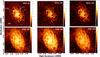 |
Fig. 1 Spitzer MIPS-24 μm (upper left panel), Herschel PACS-100 and 160 μm (upper middle and right panels, respectively) and SPIRE-250, 350, and 500 μm (lower left, middle and right panels, respectively). All maps are at their original resolution, and the FWHM of the beams (6′′, 6.7″ × 6.9″, 10.7″ × 11.1″, 18.3″ × 17.0″, 24.7″ × 23.2″, and 37.0″ × 33.4″ for 24, 100, 160, 250, 350, and 500 μm respectively) are indicated as green circles at the bottom-left part in each panel. In the MIPS-24 μm map, three of the brightest HII regions are labeled for reference. The outer ellipse shows the B-band D25 (semi-major axis length = 7.5 kpc; Paturel et al. 2003) extent of the galaxy. The brightness scale is given in units of MJy sr-1. |
Owing to their proximity, the galaxies in the Local Group are ideal systems for carrying out high spatial resolution studies of the ISM. As an Sc spiral galaxy at a distance of 840 kpc (Freedman et al. 1991), M 33 is an ideal candidate for the present analysis. Previously mapped by ISO at 60, 100, and 170 μm at a moderate resolution, M 33 reveals a spiral structure with a large number of distinct sources, as well as a diffuse extended component (Hippelein et al. 2003). In the same study, spectral energy distributions (SEDs) constructed for the central part of the galaxy as well as the interarm regions and prominent HII regions, reveal typical temperatures of Tw ~ 46 K for the warm dust and Tc ~ 17 K for the cool dust component. Performing a multi-scale study of the infrared (IR) emission of M 33 using Spitzer-MIPS data and a wavelet analysis technique, Tabatabaei et al. (2007a) concluded that most of the 24 μm and 70 μm emission emerge from bright HII regions and star-forming complexes, while the 160 μm emission traces both compact and diffuse emission throughout the galaxy. Using intensity maps at 70 μm and 160 μm, Tabatabaei et al. (2007b) constructed temperature maps that illustrated the variations in the temperature of between 19 K and 28 K, while similar conclusions were reached by Verley et al. (2008) by constructing the dust temperature variations as a function of radius from the center.
The recently launched Herschel Space Observatory offers the possibility to study M 33 at FIR and submm wavelengths in more detail than possible before. The PACS (Poglitsch et al. 2010) and SPIRE (Griffin et al. 2010) instruments combined allow us to produce images over the wavelength range between 70 μm and 500 μm with unprecedented sensitivity and superior resolution. In this paper, we use PACS (100 μm and 160 μm) and SPIRE (250 μm, 350 μm, 500 μm) imaging, taken as part of the Herschel M 33 extended survey (HerM33es; Kramer et al. 2010), an open-time key program, along with a two-component modified blackbody model in order to improve our understanding of the nature of the continuum emission of M 33. With this approach, we hope to shed some light on the temperature and luminosity distributions of M 33, being aware of the simplistic nature of the model that is used. A more realistic analysis (within the framework of the HerM33es open-time key program) is presented elsewhere (Rosolowsky et al., in prep). In Sect. 2, we present the observations and the data reduction techniques that we use, Sect. 3 gives a brief description of the morphology of the galaxy at the Herschel wavelengths, Sect. 4 describes the modeling of the data, and the results of our study are presented in Sect. 5 and discussed in Sect. 6. We finally present our conclusions in Sect. 7.
2. Observations and data reduction
The Local Group galaxy M 33 was observed on 7 and 8 January 2010 with PACS and SPIRE covering a field of 70′ × 70′. Observations were made using the PACS and SPIRE parallel mode with a scanning speed of 20″/s providing simultaneous observations at 100 μm and 160 μm, as well as at 250 μm, 350 μm, and 500 μm. The PACS maps presented in this paper were reduced using the scanamorphos algorithm (Roussel 2012) discussed in detail in Boquien et al. (2011) and in Rosolowsky et al. (in prep.). The SPIRE maps were reduced using HIPE 7.0 (Ott 2010) and the SPIRE calibration tree v. 7.0. SPIRE characteristics (point spread function, beam area, bandpass transmission curves, and correction factors for extended emission) were taken from the SPIRE Observers’ Manual (v2.4 2011). A baseline algorithm (Bendo et al. 2010) was applied to every scan of the maps in order to correct for offsets between the detector timelines and remove residual baseline signals. Finally, the maps were created using a “naive” mapping projection. Regarding the errors in the PACS and SPIRE photometry, we adopted a conservative 15% calibration uncertainty for extended emission (Boquien et al. 2011; SPIRE Observers’ Manual, v2.4 2011).
In addition to the Herschel maps, we also used the publicly available mid-infrared (MIR) maps at 5.8 μm and 8 μm obtained with the IRAC instrument, and the 24 μm and 70 μm obtained with the MIPS instrument on-board the Spitzer Space Observatory. To account for the stellar pollution in the 5.8 μm and 8 μm fluxes, we used the IRAC-3.6 μm data as a reference point assuming that fluxes at this waveband only trace stellar emission. This, however, is a crude approximation since dust contamination, especially in the bright HII regions, may be present in 3.6 μm. We then corrected the 5.8 μm and 8 μm maps by assuming a stellar light contamination dictated by the 3.6 μm measurements scaled by a Rayleigh-Jeans law.
The maps used in our analysis had all been convolved to a common angular resolution (the resolution of the 500 μm SPIRE image; approximately 40′′) by using the dedicated convolution kernels provided by Aniano et al. (2011)1, and then projected onto the same grid (of a 10′′ pixel) and central position.
3. Morphology
Figure 1 shows the maps obtained at the five Herschel wavelengths (100, 160, 250, 350, and 500 μm) as well as the 24 μm map for comparison. In the 24 μm map, we have also indicated the B-band D25 (7.5 kpc; Paturel et al. 2003) extent of the galaxy, as well as the three of the brightest HII regions. All maps are at their original resolution and the brightness scale is in MJy sr-1.
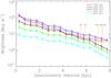 |
Fig. 2 Azimuthally averaged radial profiles, projected onto the major axis of M 33 for the 100, 160, 250, 350, and 500 μm emission (red, blue, black, green, and cyan colors, respectively). The vertical dotted lines (in orange color) indicate the 3-σ flux level threshold for each wavelength. |
We used the Herschel maps to spatially model the SED across the galaxy (see Sect. 4). All Herschel maps clearly show the spiral arm structure and a large number of distinct sources. In addition to the spiral structure, an underlying extended emission component can be recognized, particularly in the three SPIRE maps and even more clearly in the azimuthally averaged radial profiles presented in Fig. 2. These profiles correspond to average fluxes within successive elliptical rings of 500 pc width and a minor-to-major axis ratio of 0.54 accounting for an inclination of 56 degrees (Regan & Vogel 1994). The profiles are plotted all the way out to 8 kpc with the orange vertical lines indicating the 3-σ threshold in each band. We fitted to these profiles exponential functions (by minimizing the χ2), in order to derive the characteristic scalelength of the dust emission at each wavelength. We did this for the range of radii with fluxes above the 3-σ threshold. We inferred scalelengths of 1.84 ± 0.12 kpc, 2.08 ± 0.09 kpc, 2.14 ± 0.08 kpc, 2.50 ± 0.12 kpc, and 3.04 ± 0.15 kpc for the 100 μm, 160 μm, 250 μm, 350 μm, and 500 μm images, respectively. The scalelength that we derived for the 160 μm emission using the Herschel-PACS data is in excellent agreement with the value obtained using the Spitzer-MIPS data (1.99 ± 0.02 kpc; Verley et al. 2009). The flatter dust distribution at longer wavelengths is indicative of a more extended distribution related to emission dominated by “cool” (~15 K) dust grains (see Sect. 6.1). Similar conclusions have been reached by others using ISO (e.g., Alton et al. 1998; Davies et al. 1999) and Herschel (e.g., Bendo et al. 2012) observations.
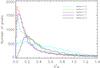 |
Fig. 3 Histogram of the |
The spiral arms detected at all Herschel bands can be traced all the way to the center of the galaxy (to a 30 pc scale; which is roughly the PACS 100 μm resolution). Two main spiral arms, one to the north-east and one to the south-west, are the brightest large-scale features of the galaxy. The main spiral structure is also present at optical, near-infrared (NIR), and radio wavelengths (Block et al. 2007; Tabatabaei et al. 2007b). Apart from these two open spiral arms, our observations show numerous, apparently independent, long-arm spiral features in the outer regions of the galaxy, that have a smaller pitch angle. These features form a flocculent spiral structure, while in the NIR two arcs or wound-up spiral arms delineate another coherent pattern. M 33 is not the only galaxy to have a flocculent spiral structure in young tracers, such as gas and young stars, superposed on a more grand-design spiral structure (e.g. Block et al. 1996). These branched multiple spirals could be random and independent wave packets triggered by local gravitational instabilities in the gas and stars (Binney & Tremaine 1987) or they could result entirely from propagating star formation and differential rotation (Gerola & Seiden 1978). In this case, gaseous instabilities trigger a first episode of star formation leading to supernova explosions and shell-like compressions in the ISM. This triggers additional star formation leading to a chain reaction in which aggregates of stars are created (see, e.g., Verley et al. 2010). The differential rotation of the galaxy, then, stretches these aggregates into spiral arcs. A characteristic picture of these violent processes is also evident in M 33 in terms of a huge (>1 kpc) shell-like feature that appears to break the south-west spiral arm (which is clearly evident in all Herschel maps of Fig. 1). A detailed analysis of the morphology of the gas and dust content of M 33 is presented in Combes et al. (2012) using power-spectrum analysis techniques.
This picture is in excellent agreement with other tracers of the ISM such as the atomic and the molecular hydrogen (Braine et al. 2010; Gratier et al. 2010, 2012). Many localized IR sources are well-detected in the Herschel bands. These sources are mainly HII regions situated in the spiral arms showing enhanced star-formation activity. A detailed analysis of the properties of these sources is presented in Verley et al. (2010) as well as in Boquien et al. (2010).
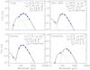 |
Fig. 4 Spectral energy distributions for the total galaxy (upper left panel) and a typical HII region (upper right – center of NGC 604), as well as the center of the galaxy (lower left panel) and the “diffuse” outer part of the galaxy (lower right panel). The emission was modeled with two modified blackbodies of β = 1.5 and fitted to the MIPS 24 and 70 μm, PACS 100 and 160 μm, and SPIRE 250, 350, and 500 μm observations. For the bright parts of the galaxy (around the center and in bright HII regions), it is evident that the specific model is unable to accurately describe the data giving unphysically high temperatures for the “warm” dust component. In the text, we describe two different and more reliable methods to derive the properties of the “warm” dust component (see Sect. 4.1 for more details). |
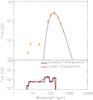 |
Fig. 5 Two of the techniques adopted to estimate the “warm” dust luminosity. After computing the “cool” dust component (top panel), the residual MIR, FIR, and submm fluxes were calculated (blue points in the bottom panel). These residual fluxes were then integrated using (a) constant values within specified wavelength ranges according to the filter passbands (black lines) and (b) a linear interpolation between successive measurements (red lines). The pixel used for this demonstration is centered at 01:34:14.64, +30:34:31.57. |
4. The model
The unprecedented spatial resolution in the FIR and submm wavelengths obtained with Herschel allows us to study the dust grain properties on a very small scale throughout the galaxy. For this purpose, the dust SED was modeled assuming optically thin emission described by two modified blackbodies, one accounting for the “cool” dust emission, originating from the large grains being heated by the local and the diffuse galactic radiation field, and one accounting for the “warm” dust emission, originating from the grains being heated in dense and warm environments where star formation is taking place. According to this model, the emission at a given frequency (ν) is described by ![Mathematical equation: \begin{eqnarray} {S}_{\nu} &=& \frac{1}{\lambda^{\beta}} [N_{\rm c}B({\nu},T_{\rm c}) + N_{\rm w}B({\nu},T_{\rm w})], \end{eqnarray}](/articles/aa/full_html/2012/07/aa19291-12/aa19291-12-eq29.png) (1)where B(ν,T) is the Planck function, and Tc and Tw are the dust temperatures for the “cool” and the “warm” dust component, respectively, β is the emissivity index, and both Nc and Nw are normalization constants related to the dust column density in each of the “cool” and the “warm” components, respectively. To find the best-fit SED for each pixel on the map, our code minimizes the χ2 function (χ2 = ∑ ((Sν,obs − Sν)/ΔSν,obs)2) using the Levenberg-Marquardt algorithm (Bevington & Robinson 1992). The model was applied to the 24, 70, 100, 160, 250, 350, and 500 μm maps regridded to a common resolution and pixel size (see Sect. 2) and for all pixels with intensities higher than three times the root mean square (rms) noise level. The rms noise level for the (FWHM = 40′′ and pixel size = 10′′) maps that we used are 0.012, 0.31, 3.2, 3.4, 0.64, 0.50, and 0.32 mJy pix-1 for the 24, 70, 100, 160, 250, 350, and 500 μm respectively. These values were obtained by performing the statistics in regions well outside the galaxy. To expand our modeling to fainter parts of the galaxy (further than the distances allowed by the 3-σ criterium to all available observations), we constrained the model by using the 24, 70, 250, 350, and 500 μm fluxes only (i.e., dropping the low signal-to-noise 100 and 160 μm measurements in the outer parts of the galaxy). These signal-to-noise considerations allowed 47% of the galaxy’s area to be modeled by using the full dataset (seven wavelengths), while for the remaining 53% (mostly the outermost parts of the galaxy), the model was constrained by measurements at five wavelengths. We note here that, at that point of the analysis, we made no use of the 5.8 and 8 μm fluxes to constrain the model. These observations were instead used later to calculate the “warm” dust component of the SED (see Sect. 4.1). To adjust for the filter bandpasses, the SED was convolved with the filter transmission before entering the χ2 minimization process. On the basis of the χ2 minimization, we derived best-fit temperatures and luminosity densities.
(1)where B(ν,T) is the Planck function, and Tc and Tw are the dust temperatures for the “cool” and the “warm” dust component, respectively, β is the emissivity index, and both Nc and Nw are normalization constants related to the dust column density in each of the “cool” and the “warm” components, respectively. To find the best-fit SED for each pixel on the map, our code minimizes the χ2 function (χ2 = ∑ ((Sν,obs − Sν)/ΔSν,obs)2) using the Levenberg-Marquardt algorithm (Bevington & Robinson 1992). The model was applied to the 24, 70, 100, 160, 250, 350, and 500 μm maps regridded to a common resolution and pixel size (see Sect. 2) and for all pixels with intensities higher than three times the root mean square (rms) noise level. The rms noise level for the (FWHM = 40′′ and pixel size = 10′′) maps that we used are 0.012, 0.31, 3.2, 3.4, 0.64, 0.50, and 0.32 mJy pix-1 for the 24, 70, 100, 160, 250, 350, and 500 μm respectively. These values were obtained by performing the statistics in regions well outside the galaxy. To expand our modeling to fainter parts of the galaxy (further than the distances allowed by the 3-σ criterium to all available observations), we constrained the model by using the 24, 70, 250, 350, and 500 μm fluxes only (i.e., dropping the low signal-to-noise 100 and 160 μm measurements in the outer parts of the galaxy). These signal-to-noise considerations allowed 47% of the galaxy’s area to be modeled by using the full dataset (seven wavelengths), while for the remaining 53% (mostly the outermost parts of the galaxy), the model was constrained by measurements at five wavelengths. We note here that, at that point of the analysis, we made no use of the 5.8 and 8 μm fluxes to constrain the model. These observations were instead used later to calculate the “warm” dust component of the SED (see Sect. 4.1). To adjust for the filter bandpasses, the SED was convolved with the filter transmission before entering the χ2 minimization process. On the basis of the χ2 minimization, we derived best-fit temperatures and luminosity densities.
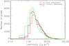 |
Fig. 6 The histogram of the luminosity densities of M 33 produced by the “cool” dust component (green) and the “warm” dust component (red and black). The “cool” part of the luminosity was derived by fitting the SED with a two-component modified blackbody (β = 1.5) model. The “warm” part of the luminosity is computed using the residual fluxes of the SED, derived after subtracting the “cool” dust component (see Fig. 5), and by adopting two approximations consisting of integrating the residual SED by a constant interpolation (black line) and a linear interpolation (red line) between the successive fluxes (see the text for more details). |
To compute the uncertainty in the derived parameters, we fitted the model to fluxes obtained within the uncertainty range of the observed fluxes. This was done by generating a series of random deviates with a normal distribution (centered on the observed flux; Press et al. 1986). We created 2000 of these mock datasets which, after fitting the SED model, resulted in a set of 2000 values for each fitted parameter. From this distribution, the 90% confidence intervals were determined and both lower and upper limits were assigned to the best-fit value of each parameter.
The model dependence on the dust emissivity index β was first explored by examining the change in χ2 for different β values. Figure 3 shows the histogram of the reduced  values (the χ2 divided by the number of observed parameters minus the number of the fitted parameters minus one) for β = 1, 1.3, 1.5, 1.7, and 2. From this plot, it is evident that the values close to β = 1.5 account for more points corresponding to the minimum value of , which implies that there is a closer match between observations and the model within the error variance of the data. The peak values of the histograms correspond to values of of ~0.17, 0.02, 0.02, 0.06, and 0.19 for β = 1, 1.3, 1.5, 1.7, and 2, respectively, with the β = 1.5 distribution being the narrowest one. This value of β is in good agreement with the best-fit value found by Kramer et al. (2010) in azimuthally averaged fluxes in elliptical rings. It is also in good agreement with statistical studies of galaxies (e.g., Dunne & Eales 2001; Yang & Phillips 2007; Benford & Staguhn 2008). A comprehensive analysis of the dust emission dependence on β (within the framework of the HerM33es Key Project) is presented elsewhere (Tabatabaei et al. 2011).
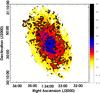 |
Fig. 7 The “cool” temperature (Tc) distribution across the galaxy. The two isothermal contours delineate regions with Tc < 18 K (yellow areas), 18 K < Tc < 23 K (red/orange areas), and Tc > 23 K (blue areas). |
4.1. The “warm” dust component of the SED
The “warm” dust component is a poorly constrained parameter of our model, because the simple model that we use is incapable of accurately describing the heating of the small dust grains emitting at short wavelengths. This is a particularly important caveat of the model when fitting bright parts of the galaxy such as the central region and the cores of the bright HII regions. In these regions, the majority of the SED can be adequately fitted by the “cool” component, leaving only one flux measurement (at 24 μm) to constrain the “warm” part of the SED. It is, nevertheless, the unphysically large values of the “warm” dust temperatures and luminosities as well as the large uncertainties in these parameters that make this model inadequate in accounting for this part of the SED. A more realistic model, taking into account dust emission at shorter, MIR, wavelengths is clearly needed for a more complete determination of the dust properties of the galaxy (Rosolowski et al., in prep.).
Typical examples of single-pixel SEDs are shown in Fig. 4. The upper right panel presents an SED near the peak of the NGC 604 HII region (01:34:34.09, +30:46:51.25), the lower left panel shows an SED at the center of the galaxy (01:33:45.21, +30:38:41.69), and a faint, diffuse part of the outskirts of the galaxy (01:32:42.54, +30:30:50.58) is presented in the lower right panel. The SED for the last position shows a typical case where only five flux measurements (PACS excluded; see Sect. 4) are used to constrain the model. From these SEDs, the lack of data points shorter than 24 μm becomes evident in the brightest parts of the galaxy (NGC 604 and center of the galaxy) with the model failing to simulate the “warm” dust emission giving unphysically high values for the temperature of this component.
To estimate the energy output of M 33 linked to the star-forming activities taking place inside the galaxy (the “warm” part of the SED), we computed the luminosity of the residual fluxes, after subtracting the well-defined “cool” component of the SED computed above; see Fig. 5. This was done on a pixel-by-pixel basis, by integrating the residual fluxes assuming a constant interpolation between successive wavelengths (see an example in Fig. 5). In particular, we assumed that the 5.8, 8, 24, 70, 100, 160, 250, 350, and 500 μm residual fluxes were constant in the wavelength ranges of 5–6.44 μm, 6.44–9.34 μm, 9.34–47 μm, 47–85 μm, 85–130 μm, 130–190 μm, 190–300 μm, 300–400 μm, and 400–1000 μm, respectively (see the residual plot in Fig. 5). The wavelength ranges for the 5.8, 8, 250, 350, and 500 μm residual fluxes were dictated by the actual width of the IRAC and SPIRE passbands, with the 500 μm range extending up to 1000 μm. For the MIPS and the PACS measurements, we used the mid-point between successive wavelengths as the wavelength limit. With this method, we computed a “warm” dust luminosity of 7.8 × 10⁸  L⊙ across the entire galaxy. We note here that the tightly constrained “cool” dust component results in a luminosity production of 1.1 × 10⁹
  L⊙.
L⊙.
To test the accuracy of this method, we also computed the “warm” dust luminosity by integrating the residual fluxes but, this time, assuming a linear interpolation for the residual fluxes at the specific wavelengths (Fig. 5). With this method, we computed a “warm” dust luminosity of 1.0 × 10⁹  L⊙. A more detailed comparison, on a pixel by pixel basis, between the two methods to determine the “warm” dust luminosity, as described above, is given in Fig. 6 with the histograms of the luminosity density (in units of L⊙ pc-2) presented for the two cases discussed above. For comparison, the histogram of the “cool” luminosity density is also plotted. From these histograms, one can see that the distribution of the luminosity densities using the two methods is very similar with the “constant” interpolation approach giving a slightly broader distribution than the “linear” one.
A further check that we did in order to investigate the accuracy of our method was to compute the luminosities of the two components by using the total fluxes for the galaxy (integrated within an ellipse with a semi-major axis length of 8 kpc). With this approach, both the “cool” and the “warm” components could be calculated (see Kramer et al. 2010), resulting in a “cool” dust luminosity of 9.3 × 10⁸  L⊙ and a “warm” dust luminosity of 7.4 × 10⁸
  L⊙ (see upper left panel in Fig. 4).
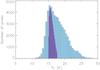 |
Fig. 8 The “cool” temperature (Tc) histogram distribution. The values derived for the whole galaxy are shown in the light blue histogram, while the dark blue only accounts for the diffuse disk of the galaxy (see Sect. 6.2). |
As a final test, we computed the total luminosity of M 33 following the recipe presented in Boquien et al. (2011). With this approach, the total IR luminosity was computed by fitting the Draine & Li model to the data (IRAC, MIPS, PACS, SPIRE). As a product of this method, scaling relations were produced between surface brightness measurements at specific wavelengths and the total IR luminosity. For our purposes, we chose to use the 250 μm surface brightness map, which is the one with the best signal-to-noise. After calculating the total IR luminosity and subtracting the already estimated “cool” dust luminosity, we found a “warm” luminosity of 8.4 × 10⁸ L⊙.
Given the large differences between the methods discussed above, the values for the “warm” dust luminosity are very similar, within the computed uncertainties, giving us great confidence that this part of the luminosity, although estimated with very simple methods, is an accurate first approximation. In our subsequent analysis, we used the luminosity calculations derived with the “constant” interpolation method since with this method the total “warm” luminosity is closer to the values derived by both the Boquien et al. (2011) method and the integrated fluxes method. With this method, the total luminosity of the galaxy (integrated in the 5–1000 μm wavelength range) is 1.9 × 10⁹  L⊙.
L⊙.
5. Results
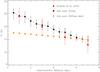 |
Fig. 9 Azimuthally averaged radial profile of the “cool” temperature for the whole galaxy (black sqares) and the disk only (orange squares; see Sect. 6.2). For comparison, the “cool” dust temperatures for the dust that were calculated in Kramer et al. (2010) for a two-component modified blackbody model with β = 1.5 and the radial anulii 0 < R < 2 kpc, 2 < R < 4 kpc, and 4 < R < 6 kpc are also presented (red triangles). |
Figure 7 shows the “cool” temperature pixel map created by modeling the SED. This dust component is heated to temperatures of between 11 K and 28 K with ~15 K being the most common temperature throughout the galaxy (see Fig. 8). In general, the “cool” temperature is symmetrically distributed throughout M 33 with typical temperatures of ~25 K close to the center of the galaxy, dropping to ~15 K close to the outskirts. The spiral structure can not be clearly seen in the “cool” temperature distribution (Fig. 7). The effect of the dimming of the spiral arms with respect to the large radial gradient of the galaxy is also present when looking at the 250/350 and 500/350 color maps (with the SPIRE colors being valuable indicators of the “cool” dust temperature distribution; see Fig. 4 in Boquien et al. 2011; and Fig. 1 in Braine et al. 2010). This is also evident when looking at the azimuthally averaged profile of the temperature (black line in Fig. 9), which undergoes a monotonic decrease from the center to the outskirts with no obvious variations from, e.g., the spiral structure. For comparison, the “cool” dust temperature values calculated by Kramer et al. (2010) but for a range of elliptical annuli are also plotted (red triangles). In general, the values are within the errors in the temperature. The slightly higher temperatures that we calculate are due to the small differences in the calibration of the Herschel data set used in Kramer et al. (2010).
Temperatures of T < 18 K (yellow areas in Fig. 7) are found in the outer parts of the galaxy, while higher temperatures are found in the inner parts of the galaxy. The highest temperatures (T > 23 K; innermost contour; blue areas in Fig. 7) are found in individual HII regions and at the center of the galaxy. This picture is also evident when examining individual SEDs similar to the ones presented in Fig. 4 with temperatures in the ranges discussed above for the HII regions (e.g., NGC 604), the center of the galaxy, and the diffuse outskirt regions of the galaxy. In these cases, the best-fit temperatures and the 90% confidence limits obtained with this model are  K for the NGC 604 region,
  K for the central region of the galaxy, and
  K in the outer, diffuse parts of the galaxy. These are typical temperatures for the various regions throughout the galaxy, which also provide an estimate of the accuracy of the fitted parameters. Given the simplicity of our SED model, especially at MIR wavelengths (those shorter than ~70 μm), where significant contribution to the emission from stochastically heated dust grains is expected, we investigated the effects of omitting the 70 μm fluxes from the analysis. In this way, the “cool” dust component was constrained by observations at wavelengths longer than 100 μm. We found that the “cool” dust temperature varies only slightly (by less than 2%), which is well within the estimated uncertainties. This gives us sufficient confidence in our “cool” dust component calculation.
For the “warm” dust component, we do not present a temperature map since, as already stressed before, the temperature of this component derived from the two modified-blackbody fit, is highly uncertain in many regions throughout the galaxy (especially the bright ones; see the upper right and lower left panels in Fig. 4). It is worth mentioning however that, when considering the galaxy as a whole, the “warm” dust temperature can be calculated, and is  K (in accordance with previous studies, e.g., Kramer et al. 2010) while for a typical, low brightness region (similar to the one in the lower right panel of Fig. 4), the temperature is
  K.
K.
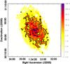 |
Fig. 10 The luminosity map of M 33 produced by the “cool” dust grains. Luminosities fainter than 7 L⊙ pc-2 (yellow areas) are found in the outer diffuse parts of the galaxy, while higher luminosities trace the spiral arms (orange/red areas). The highest luminosity densities (>90 L⊙ pc-2; innermost contours; blue areas) are produced in the bright HII regions and the center of the galaxy. |
The “cool” dust luminosity (Figs. 6 and 10) varies between ~0.3 L⊙ pc-2 and ~800 L⊙ pc-2 with a value of ~1.7 L⊙ pc-2 accounting for most parts of the galaxy. Luminosities fainter than 7 L⊙ pc-2 (yellow areas in Fig. 10) were detected for the diffuse parts of the outermost regions of the galaxy, while higher luminosities (orange/red areas in Fig. 10) are emitted from the spiral arms. The highest luminosity densities (L > 90 L⊙ pc-2; innermost contours (blue areas) in Fig. 10) are produced by the HII regions and the center of the galaxy. This is also evident when examining the individual SEDs for different regions of the galaxy (Fig. 4), resulting in a “cool” dust luminosity of  L⊙ pc-2 for NGC 604, one of
  L⊙ pc-2 for the center, and
  L⊙ pc-2 for the outer parts of the galaxy.
The “warm” dust luminosity (Figs. 6 and 11) varies between ~0.3 L⊙ pc-2 and ~400 L⊙ pc-2 with a value of ~1.6 L⊙ pc-2 accounting for most parts of the galaxy. Luminosities less than 7 L⊙ pc-2 (yellow areas in Fig. 11) are produced in the diffuse parts of the galaxy while higher luminosities are emitted from the spiral arms (orange/red areas in Fig. 11). The highest luminosity densities (L > 40 L⊙ pc-2; innermost contours (blue areas) in Fig. 11) are produced by the HII regions and the center of the galaxy. This map was computed by applying the “constant” interpolation method for estimating the “warm” dust luminosity (see Sect. 4.1). As in the case of the “cool” dust luminosity (discussed above) individual SEDs correspond to luminosities, produced by the “warm” dust material, of  L⊙ pc-2 for NGC 604,
  L⊙ pc-2 for the center of M 33, and
  L⊙ pc-2 for the outer parts of the galaxy.
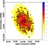 |
Fig. 11 The luminosity map of M 33 produced by the “warm” dust grains. Luminosities fainter than 6 L⊙ pc-2 (yellow areas) are found in the outer diffuse parts of the galaxy, while higher luminosities trace the spiral arms (orange/red regions). The highest luminosity densities (>40 L⊙ pc-2; innermost contours; blue areas) are produced in the bright HII regions and the center of the galaxy. The “constant” interpolation method was used to estimate the “warm” dust luminosities. |
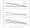 |
Fig. 12 The azimuthally averaged profiles of the “cool” and the “warm” dust luminosities (green and blue lines) in units of L⊙ pc-2. The cool-to-warm luminosity ratio is also plotted (red line). The luminosities are calculated for the whole galaxy (upper panel) and the disk of the galaxy only (middle panel; see Sect. 6.2). The residuals between the two profiles give the radial distribution of the luminosity produced by the spiral arm network (bottom panel). |
6. Discussion
6.1. The “warm” and the “cool” dust distributions
Our comparison of the “cool” and the “warm” luminosity maps in Figs. 10 and 11 indicates that the morphologies of the two dust components are very similar with the spiral structure clearly being seen in both cases and with local enhancements being found in the areas where the HII regions reside. This similarity becomes more striking when looking at the azimuthally averaged radial profiles (upper panel in Fig. 12) of the luminosity densities of the two components (green and blue lines for the “cool” and the “warm” components) and their ratio (Lc/Lw; red line). From these profiles, it is evident that, given the uncertainties in the computed luminosities, the “cool” dust luminosity is the dominant source of luminosity in the central parts of the galaxy (with the “cool” luminosity being about three times higher than the “warm” luminosity), while the ratio gets rather flat and close to unity beyond a ~3 kpc radius. This narrow range of the ratio (close to unity) of the two luminosities suggests that both dust components (the “cool” dust heated at ~15 K and the “warm” dust heated at ~55 K) are able to produce about the same luminosities throughout the galaxy.
Approximating the azimuthally averaged radial profiles of the two luminosities with exponential functions, we find that they decay with scalelengths of 2.59 ± 0.04 kpc for the “cool” dust, and 1.77 ± 0.02 kpc for the “warm” dust. Comparing with the scalelengths that we have derived for individual wavelengths (Sect. 3 and this section), we can see that the “warm” dust luminosity is very similar to the values derived for the MIR/FIR wavelengths, while the “cool” dust luminosity has a scalelength similar to the 250–500 μm submm wavelengths. This directly implies that the “cool” dust grains (which contribute mostly to the “cool” part of the luminosity of the galaxy) emit in the submm wavelengths, while the “warm” dust grains emit in the MIR/FIR wavelengths forming the “warm” part of the luminosity of the galaxy.
6.2. Decomposing M 33 into a disk and a spiral arm network
The dust distribution inside a galaxy can be quite inhomogeneous. When considering the morphology on a large scale, the dust distribution can be approximated by a superposition of a diffuse disk and a spiral arm network (see e.g. Xilouris et al. 1999; Misiriotis et al. 2000; Meijerink et al. 2005). As a first order approximation, the diffuse disk can be accurately described by a three-dimensional disk decreasing exponentially in both the radial and the vertical directions 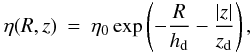 2where η0 is the dust volume density at the nucleus of the galaxy and hd and zd are the scalelength and scaleheight of the dust, respectively (see Xilouris et al. 1999). We used this simple model to delineate between the two main dust components (i.e. the dust that is diffusely distributed in a disk throughout the galaxy revealing itself in the inter-arm regions of the galaxy and the dust forming the spiral arms).
Determining the scaleheight of the dust is non-trivial since, unlike for edge-on galaxies where the vertical extent of the dust can be measured, in less-inclined galaxies, such as M 33, this parameter cannot be easily determined. We note however that in our present study, where we aim to calculate the relative fraction of the fluxes and luminosities emitted by the diffuse and the spiral arm network, the choice of the scaleheight is not a crucial issue. This is because the total luminosity of the disk is independent of zd (a larger value of zd (thicker disk) would require a smaller value of η0 (fainter disk) in order to fit the data, which, in the end, would also result in the same luminosity; see Xilouris et al. 1997). For the purposes of this study, we used a scaleheight of zd = 0.2 kpc. This is a typical scaleheight for the diffuse dust in a galaxy derived from modeling and observations of edge-on galaxies (Xilouris et al. 1999; Bianchi & Xilouris 2011). In particular, for M 33, it is close to the value derived by Combes et al. (2012) using a power-spectrum analysis.
For the scalelength, we used the values determined by fitting the azimuthally averaged profiles (see Sect. 3, Fig. 2). Since we also wished to investigate the origin of the emission at MIR wavelengths, we performed the analysis for the scalelength determination (described in Sect. 3) in the MIPS-24 μm and 70 μm data. We found scalelength values of 1.87 ± 0.09 and 1.90 ± 0.05 kpc, respectively, for the 24 μm and 70 μm emission.
With the scalelengths and scaleheights of the disk fixed, our three-dimensional model was then inclined by 56 degrees (the inclination angle of M 33) and the intensities of the model integrated along the line of sight were fitted to the galaxy maps on a pixel-by-pixel basis. We used only the fluxes in the outermost and the inter-arm regions of the galaxy (the latter areas consisting of the minimum values in-between the obvious spiral structure) to constrain the emissivity at the galactic center (η0). We did this because we only wished to fit the diffuse part of the galaxy and disregard both the spiral arms and the more complex structures superimposed on the diffuse disk. This fit was done by minimizing the χ2 values in a similar procedure with what is described in Sect. 4.
An example of this analysis is presented in Fig. 13, which illustrates the 250 μm map decomposition. In this figure, the black contours show the axisymmetric exponential disk that is fitted to the data (Eq. (2)), while the red contours show the spiral arm network determined after subtracting the map of the diffuse disk from the observed image. This decomposition can be seen in more detail in Fig. 14, where we present the radial profiles of the disk fitted to the 250 μm data (dotted lines) along with the observed major- and minor-axis profiles (left and right panel respectively). From these profiles, it is clear that the spiral arms are superimposed on the disk, allowing a clear separation of the two components.
Using the available Spitzer and Herschel maps of M 33, we found that the flux that is emitted from the disk accounts for 21, 29, 38, 42, 48, 52, and 57% of the total flux at the wavelengths 24, 70, 100, 160, 250, 350, and 500 μm, respectively. We can see that at MIR wavelengths, it is the spiral structure that is the dominant source of emission, while, at around ~250 μm the emission comes equally from the disk and the spiral arms. In contrast, the dominant source of the submm emission is the disk of the galaxy.
After calculating the emission that is produced by the diffuse dust disk in all available bands, we were then able to calculate the temperature and the luminosity of this component separately. We did so by applying the SED modeling that we had previously performed for the whole galaxy (Sect. 4) but now for this component only.
“Warm” and “cool” dust luminosities for the total galaxy, the disk of the galaxy and the spiral arms of the galaxy.
For the “cool” temperature in the disk, we found a very narrow distribution (compared to the galaxy as a whole) with values ranging between 15 K and 18 K. This is indicated in Fig. 8 by the dark blue distribution being that of the diffuse disk. Given a typical 3 K uncertainty in the temperature distribution, the disk temperatures occupy the lower end of the temperature distribution for the whole galaxy (light blue), leaving the higher temperatures (>18 K) accounting for the rest of the galaxy (spiral arms and HII regions). The narrow range of temperatures is also seen in Fig. 9, with temperatures of ~18 K occuring at the center of the galaxy dropping to ~15 K at the edges. A similarly narrow range of temperatures for the diffuse dust in the disk of the Milky Way was derived based on COBE observations. Temperatures for the diffuse cirrus component ranging from 17 K to 21 K were found using FIR color maps (e.g. Reach et al. 1995; Schlegel et al. 1998), while a 15 K to 19 K range was computed for the disk of the Milky Way via radiative transfer modeling (Misiriotis et al. 2006). Similar findings were derived using Herschel observations of the Galactic plane indicating that the warmest dust is located in the spiral arms (Bernard et al. 2010). The narrow range of the temperatures that we measured for the disk of M 33 is consistent with this picture, with the disk primarily hosting the cirrus dust component, which is in turn heated by the diffuse interstellar radiation field. On the other hand, the dust in the spiral arms is embedded in more dense environments, and is mainly heated by the local ultraviolet radiation of the young stars, leading to a wider range of temperatures. We note however that a more detailed analysis, taking into account both the exact radiation field heating the dust as well as the dust composition and density in various places throughout the galaxy, is clearly needed for a proper characterization of the properties of the interstellar dust in different environments.
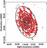 |
Fig. 13 The 250 μm image of M 33 decomposed into a diffuse axisymmetric disk (black contours) and a spiral structure network (red contours; see the text for more details). |
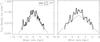 |
Fig. 14 The 250 μm profile of M 33 along both the major axis (left) and the minor axis (right). In both cases, the solid line corresponds to the observed emission, while the dotted line is the exponential disk fitted to the data. |
Concerning the luminosity, we find that 5.7 × 10⁸ L⊙ (30% of the total luminosity) is produced by the dust in the disk. This indicates that the dominant source of the luminosity of the galaxy at IR/submm wavelengths is the spiral arm network. Furthermore, considering the “warm” and the “cool” components separately we computed that the dust that resides in the disk and is “warm” emits a luminosity of 2.5 × 10⁸ L⊙, which is 32% of the total “warm” dust luminosity, while the “cool” dust material produces 3.2 × 10⁸ L⊙, which is 29% of the total “cool” dust luminosity. All the above results, as well as the values derived for the spiral arms, are summarized in Table 1.
The above results indicate that the luminosities of the “warm” and the “cool” dust appear to originate mainly in the spiral arm network, which produces 71% of the luminosity of the “cool” and 68% of the luminosity of the “warm” dust of the galaxy. Furthermore, 41% of the total luminosity of the galaxy is emitted by “warm” grains, while the remaining 59% is emitted by “cool” dust grains. These percentages are about the same when separating the disk from the spiral arms. For example, we see that inside the disk 44% of the luminosity is emitted by the “warm” dust, whereas 56% is emitted by the “cool” dust; similarly for the spiral arms, 40% comes from the “warm” and 60% from the “cool” dust.
It is also interesting to investigate the relative distributions of the “warm” and “cool” luminosities that reside inside the disk and the spiral arms as a function of galactocentric radius. The decomposition of the azimuthally averaged radial profiles is shown in Fig. 12, with the disk profiles presented in the middle panel and the spiral arm profiles in the bottom panel. The disk profiles (middle panel) are derived by fitting the two modified-blackbody model to the smooth disk maps at each available wavelength. These maps are derived by fitting the three-dimensional model (Eq. (2)) to the observations as described earlier. From these profiles, it is evident that the “cool” dust in the disk of the galaxy becomes the dominant component in the outer parts of the galaxy (beyond ~3 kpc), while the “cool” dust is the main source of luminosity production within the inner ~3 kpc inside the spiral arm network.
7. Conclusions
By modeling the SED of the Local Group galaxy M 33 and exploiting the unique wavelength coverage and sensitivity of the Herschel 100, 160, 250, 350, and 500 μm observations, as well as additional Spitzer-IRAC 5.8 μm and 8 μm and Spitzer-MIPS 24 μm and 70 μm data, we have derived the following conclusions about the dust emission of the galaxy:
-
The submm emission from M 33 is distributedmore evenly (scalelength of 3.04 kpc at500 μm) than the far-infrared emission (scalelengthof 1.84 kpc at 100 μm).
-
On average, the emission by the dust can be adequately modeled by a superposition of two modified blackbodies with β = 1.5.
-
The temperature of the “cool” grains ranges between 11 K and 28 K, with a most common value of ~15 K across the galaxy.
-
The total luminosity of the galaxy (integrated from 5 to 1000 μm) is 1.9 × 10⁹
L⊙, with the luminosity of the “cool” dust component accounting for 59% of the total luminosity. -
The scalelength of the “cool” (“warm”) luminosity distribution is very similar to that of the submm (MIR/FIR) emission. This similarity directly reflects the wavelengths that contribute the most to each of the two luminosity components.
-
Decomposing the galaxy into two components (namely, a diffuse disk and a spiral-arm network), we have found that the emission in the disk accounts for ~21% of the emission at the MIR wavelengths (24 μm), while it gradually rises to ~57% at submm wavelengths (500 μm).
-
The “cool” dust material in the disk of the galaxy, presumably accounting for the cirrus dust component of the galaxy, is heated to temperatures of between ~15 K at the edges of the galaxy and ~18 K at the center.
-
The bulk of the luminosity is emitted by the spiral arm network (~70%), and this percentage stays roughly the same when considering the “warm” and the “cool” dust luminosities separately.
-
About ~40% of the total luminosity throughout the galaxy (and separately within the disk and the spiral arms) is emitted by the “warm” dust grains, with the remaining ~60% being emitted by the “cool” dust.
-
The ratio of the “cool” to “warm” dust luminosity is close to unity throughout most of the the galaxy but slightly higher within the central ~3 kpc of the galaxy.
-
The “cool” dust within the disk becomes the dominant source of the infrared emission in the outer parts of the galaxy (beyond ~3 kpc).
-
In contrast, the “cool” dust within the spiral arms become dominant in the inner parts of the galaxy (within ~3 kpc).
Acknowledgments
We are grateful to Marc Sauvage, George Bendo, Pierre Chanial, Michael Pohlen, and Richard Tuffs for their help in completing the data reduction. We also thank the anonymous referee for providing useful comments that helped to improve the paper. F.S.T. acknowledges support by the DFG via the grant TA 801/1-1.
References
- Alton, P. B., Trewhella, M., Davies, J. I., et al. 1998, A&A, 335, 807 [NASA ADS] [Google Scholar]
- Aniano, G. J., Draine, B. T., Gordon, K. D., & Sandstrom, K. 2011, PASP, 123, 1218 [NASA ADS] [CrossRef] [Google Scholar]
- Bendo, G. J., Wilson, C. D., Pohlen, M., et al. 2010, A&A, 518, L65 [NASA ADS] [CrossRef] [EDP Sciences] [Google Scholar]
- Bendo, G. J., Boselli, A., Dariush, A., et al. 2012, MNRAS, 419, 1833 [NASA ADS] [CrossRef] [Google Scholar]
- Benford, D. J., & Staguhn, J. G. 2008, ASPC, 381, 132 [NASA ADS] [Google Scholar]
- Bernard, J.-Ph., Paradis, D., Marshall, D. J., et al. 2010, A&A, 518, L88 [NASA ADS] [CrossRef] [EDP Sciences] [Google Scholar]
- Bevington, P., & Robinson, D. 1992, Data reduction and error analysis for the physical sciences (McGraw-Hill, Inc.) [Google Scholar]
- Bianchi, S., & Xilouris, E. M. 2011, A&A, 531, A11 [Google Scholar]
- Binney J., & Tremaine S. 1987, Galactic Dynamics (Princeton: Princeton Univ. Press) [Google Scholar]
- Block, D. L., Elmegreen, B. G., & Wainscoat, R. J. 1996, Nature, 381, 674 [NASA ADS] [CrossRef] [Google Scholar]
- Block, D. L., Combes, F., Puerari, I., et al. 2007, A&A, 471, 467 [NASA ADS] [CrossRef] [EDP Sciences] [Google Scholar]
- Boquien, M., Calzetti, D., Kramer, C., et al. 2010, A&A, 518, L70 [NASA ADS] [CrossRef] [EDP Sciences] [Google Scholar]
- Boquien, M., Calzetti, D., Combes, F., et al. 2011, AJ, 142, 111 [NASA ADS] [CrossRef] [Google Scholar]
- Braine, J., Gratier, P., Kramer, C., et al. 2010, A&A, 518, L69 [NASA ADS] [CrossRef] [EDP Sciences] [Google Scholar]
- Combes, F., Boquien, M., Kramer, C., et al. 2012, A&A, 539, A67 [NASA ADS] [CrossRef] [EDP Sciences] [Google Scholar]
- Davies, J. I., Alton, P., Trewhella, M., Evans, R., & Bianchi, S. 1999, MNRAS, 304, 495 [NASA ADS] [CrossRef] [Google Scholar]
- Devereux, N. A., & Young, J. S. 1990, ApJ, 359, 42 [NASA ADS] [CrossRef] [Google Scholar]
- Dunne, L., & Eales, S. A. 2001, MNRAS, 327, 697 [NASA ADS] [CrossRef] [Google Scholar]
- Freedman, W. L., Wilson, C. D., & Madore, B. F. 1991, ApJ, 372, 455 [NASA ADS] [CrossRef] [Google Scholar]
- Gerola, H., & Seiden, P. E. 1978, ApJ, 223, 129 [NASA ADS] [CrossRef] [Google Scholar]
- Gordon, K. D., Bailin, J., Engelbracht, C. W., et al. 2006, ApJ, 638, 87 [Google Scholar]
- Gratier, P., Braine, J., Rodriguez-Fernandez, N. J., et al. 2010, A&A, 522, A3 [NASA ADS] [CrossRef] [EDP Sciences] [Google Scholar]
- Gratier, P., Braine, J., Rodriguez-Fernandez, N. J., et al. 2012, A&A, 542, A108 [NASA ADS] [CrossRef] [EDP Sciences] [Google Scholar]
- Griffin, M., Abergel, A., Abreu, A., et al. 2010, A&A, 518, L3 [Google Scholar]
- Haas, M., Lemke, D., Stickel, M., et al. 1998, A&A, 338, 33 [NASA ADS] [Google Scholar]
- Hippelein, H., Haas, M., Tuffs, R. J., et al. 2003, A&A, 407, 137 [NASA ADS] [CrossRef] [EDP Sciences] [Google Scholar]
- Hoopes, C. G., & Walterbos, R. A. M. 2000, ApJ, 541, 597 [NASA ADS] [CrossRef] [Google Scholar]
- Kramer, C., Richer, J., Mookerjea, B., Alves, J., & Lada, C. 2003, A&A, 399, 1073 [NASA ADS] [CrossRef] [EDP Sciences] [Google Scholar]
- Kramer, C., Buchbender, C., Xilouris, E. M., et al. 2010, A&A, 518, L67 [NASA ADS] [CrossRef] [EDP Sciences] [Google Scholar]
- Krüegel, E. 2003, The physics of interstellar dust, ed. E. Krüegel [Google Scholar]
- Krüegel, E., & Siebenmorgen, R. 1994, A&A, 288, 929 [NASA ADS] [Google Scholar]
- Meijerink, R., Tilanus, R. P. J., Dullemond, C. P., Israel, F. P., & van der Werf, P. P. 2005, A&A, 430, 427 [NASA ADS] [CrossRef] [EDP Sciences] [Google Scholar]
- Misiriotis, A., Kylafis, N. D., Papamastorakis, J., & Xilouris, E. M. 2000, A&A, 353, 117 [NASA ADS] [Google Scholar]
- Ott, D. 2010, ASP Conf. Ser., 434, 139 [Google Scholar]
- Paturel, G., Petit, C., Prugniel, P., et al. 2003, A&A, 412, 45 [NASA ADS] [CrossRef] [EDP Sciences] [Google Scholar]
- Pilbratt, G. L., Riedinger, J. R., Passvogel, T., et al. 2010, A&A, 518, L1 [CrossRef] [EDP Sciences] [Google Scholar]
- Poglitsch, A., Waelkens, C., Geis, N., et al. 2010, A&A, 518, L2 [NASA ADS] [CrossRef] [EDP Sciences] [Google Scholar]
- Press, W. H., Flannery, B. P., Tenkolsky, S. A., & Vetterling, W. T. 1986, Numerical Recipes (Cambridge: Cambridge Univ. Press) [Google Scholar]
- Reach, W. T., Dwek, E., Fixsen, D. J., et al. 1995, ApJ, 451, 188 [NASA ADS] [CrossRef] [Google Scholar]
- Regan, M. W., & Vogel, S. N. 1994, ApJ, 434, 536 [NASA ADS] [CrossRef] [Google Scholar]
- Roussel, H. 2012, A&A, submitted [Google Scholar]
- Schlegel, D. J., Finkbeiner, D. P., & Davis, M. 1998, ApJ, 500, 525 [NASA ADS] [CrossRef] [Google Scholar]
- Tabatabaei, F. S., Beck, R., Krause, M., et al. 2007a, A&A, 466, 509 [NASA ADS] [CrossRef] [EDP Sciences] [Google Scholar]
- Tabatabaei, F. S., Beck, R., Krügel, E., et al. 2007b, A&A, 475, 133 [NASA ADS] [CrossRef] [EDP Sciences] [Google Scholar]
- Tabatabaei, F. S., Braine, J., Kramer, C., et al. 2011, Proc. IAU Symp. 284, eds. R. J. Tiffs, & C. C. Popescu [Google Scholar]
- Verley, S., Hunt, L. K., Corbelli, E., & Giovanardi, C. 2007, A&A, 476, 1161 [NASA ADS] [CrossRef] [EDP Sciences] [Google Scholar]
- Verley, S., Corbelli, E., Giovanardi, C., & Hunt, L. K. 2009, A&A, 493, 453 [NASA ADS] [CrossRef] [EDP Sciences] [Google Scholar]
- Verley, S., Relaño, M., Kramer, C., et al. 2010, A&A, 518, L68 [NASA ADS] [CrossRef] [EDP Sciences] [Google Scholar]
- Xilouris, E. M., Byun, Y. I., Kylafis, N. D., Paleologou, E. V., & Papamastorakis, J. 1999, A&A, 344, 868 [NASA ADS] [Google Scholar]
- Yang, M., & Phillips, T. 2007, ApJ, 662, 284 [NASA ADS] [CrossRef] [Google Scholar]
- Young, J. S., Allen, L., Kenney, J. D. P., Lesser, A., & Rownd, B. 1996, AJ, 112, 1903 [NASA ADS] [CrossRef] [Google Scholar]
All Tables
“Warm” and “cool” dust luminosities for the total galaxy, the disk of the galaxy and the spiral arms of the galaxy.
All Figures
|
Fig. 1 Spitzer MIPS-24 μm (upper left panel), Herschel PACS-100 and 160 μm (upper middle and right panels, respectively) and SPIRE-250, 350, and 500 μm (lower left, middle and right panels, respectively). All maps are at their original resolution, and the FWHM of the beams (6′′, 6.7″ × 6.9″, 10.7″ × 11.1″, 18.3″ × 17.0″, 24.7″ × 23.2″, and 37.0″ × 33.4″ for 24, 100, 160, 250, 350, and 500 μm respectively) are indicated as green circles at the bottom-left part in each panel. In the MIPS-24 μm map, three of the brightest HII regions are labeled for reference. The outer ellipse shows the B-band D25 (semi-major axis length = 7.5 kpc; Paturel et al. 2003) extent of the galaxy. The brightness scale is given in units of MJy sr-1. |
| In the text | |
|
Fig. 2 Azimuthally averaged radial profiles, projected onto the major axis of M 33 for the 100, 160, 250, 350, and 500 μm emission (red, blue, black, green, and cyan colors, respectively). The vertical dotted lines (in orange color) indicate the 3-σ flux level threshold for each wavelength. |
| In the text | |
|
Fig. 3 Histogram of the |
| In the text | |
|
Fig. 4 Spectral energy distributions for the total galaxy (upper left panel) and a typical HII region (upper right – center of NGC 604), as well as the center of the galaxy (lower left panel) and the “diffuse” outer part of the galaxy (lower right panel). The emission was modeled with two modified blackbodies of β = 1.5 and fitted to the MIPS 24 and 70 μm, PACS 100 and 160 μm, and SPIRE 250, 350, and 500 μm observations. For the bright parts of the galaxy (around the center and in bright HII regions), it is evident that the specific model is unable to accurately describe the data giving unphysically high temperatures for the “warm” dust component. In the text, we describe two different and more reliable methods to derive the properties of the “warm” dust component (see Sect. 4.1 for more details). |
| In the text | |
|
Fig. 5 Two of the techniques adopted to estimate the “warm” dust luminosity. After computing the “cool” dust component (top panel), the residual MIR, FIR, and submm fluxes were calculated (blue points in the bottom panel). These residual fluxes were then integrated using (a) constant values within specified wavelength ranges according to the filter passbands (black lines) and (b) a linear interpolation between successive measurements (red lines). The pixel used for this demonstration is centered at 01:34:14.64, +30:34:31.57. |
| In the text | |
|
Fig. 6 The histogram of the luminosity densities of M 33 produced by the “cool” dust component (green) and the “warm” dust component (red and black). The “cool” part of the luminosity was derived by fitting the SED with a two-component modified blackbody (β = 1.5) model. The “warm” part of the luminosity is computed using the residual fluxes of the SED, derived after subtracting the “cool” dust component (see Fig. 5), and by adopting two approximations consisting of integrating the residual SED by a constant interpolation (black line) and a linear interpolation (red line) between the successive fluxes (see the text for more details). |
| In the text | |
|
Fig. 7 The “cool” temperature (Tc) distribution across the galaxy. The two isothermal contours delineate regions with Tc < 18 K (yellow areas), 18 K < Tc < 23 K (red/orange areas), and Tc > 23 K (blue areas). |
| In the text | |
|
Fig. 8 The “cool” temperature (Tc) histogram distribution. The values derived for the whole galaxy are shown in the light blue histogram, while the dark blue only accounts for the diffuse disk of the galaxy (see Sect. 6.2). |
| In the text | |
|
Fig. 9 Azimuthally averaged radial profile of the “cool” temperature for the whole galaxy (black sqares) and the disk only (orange squares; see Sect. 6.2). For comparison, the “cool” dust temperatures for the dust that were calculated in Kramer et al. (2010) for a two-component modified blackbody model with β = 1.5 and the radial anulii 0 < R < 2 kpc, 2 < R < 4 kpc, and 4 < R < 6 kpc are also presented (red triangles). |
| In the text | |
|
Fig. 10 The luminosity map of M 33 produced by the “cool” dust grains. Luminosities fainter than 7 L⊙ pc-2 (yellow areas) are found in the outer diffuse parts of the galaxy, while higher luminosities trace the spiral arms (orange/red areas). The highest luminosity densities (>90 L⊙ pc-2; innermost contours; blue areas) are produced in the bright HII regions and the center of the galaxy. |
| In the text | |
|
Fig. 11 The luminosity map of M 33 produced by the “warm” dust grains. Luminosities fainter than 6 L⊙ pc-2 (yellow areas) are found in the outer diffuse parts of the galaxy, while higher luminosities trace the spiral arms (orange/red regions). The highest luminosity densities (>40 L⊙ pc-2; innermost contours; blue areas) are produced in the bright HII regions and the center of the galaxy. The “constant” interpolation method was used to estimate the “warm” dust luminosities. |
| In the text | |
|
Fig. 12 The azimuthally averaged profiles of the “cool” and the “warm” dust luminosities (green and blue lines) in units of L⊙ pc-2. The cool-to-warm luminosity ratio is also plotted (red line). The luminosities are calculated for the whole galaxy (upper panel) and the disk of the galaxy only (middle panel; see Sect. 6.2). The residuals between the two profiles give the radial distribution of the luminosity produced by the spiral arm network (bottom panel). |
| In the text | |
|
Fig. 13 The 250 μm image of M 33 decomposed into a diffuse axisymmetric disk (black contours) and a spiral structure network (red contours; see the text for more details). |
| In the text | |
|
Fig. 14 The 250 μm profile of M 33 along both the major axis (left) and the minor axis (right). In both cases, the solid line corresponds to the observed emission, while the dotted line is the exponential disk fitted to the data. |
| In the text | |
Current usage metrics show cumulative count of Article Views (full-text article views including HTML views, PDF and ePub downloads, according to the available data) and Abstracts Views on Vision4Press platform.
Data correspond to usage on the plateform after 2015. The current usage metrics is available 48-96 hours after online publication and is updated daily on week days.
Initial download of the metrics may take a while.