| Issue |
A&A
Volume 533, September 2011
|
|
|---|---|---|
| Article Number | A57 | |
| Number of page(s) | 21 | |
| Section | Extragalactic astronomy | |
| DOI | https://doi.org/10.1051/0004-6361/201116972 | |
| Published online | 29 August 2011 | |
High-frequency predictions for number counts and spectral properties of extragalactic radio sources. New evidence of a break at mm wavelengths in spectra of bright blazar sources⋆
1
LAL, Univ Paris-Sud, CNRS/IN2P3, Orsay, France
e-mail: tucci@lal.in2p3.fr
2
Departamento de Física, Universidad de Oviedo, c. Calvo Sotelo s/n, 33007 Oviedo, Spain
3
Research Unit associated with IFCA-CSIC, Instituto de Física de Cantabria, avda. los Castros, s/n, 39005 Santander, Spain
4
INAF – Osservatorio Astronomico di Padova, Vicolo dell’Osservatorio 5, 35122 Padova, Italy
5
International School for Advanced Studies, SISSA/ISAS, Astrophysics Sector, via Bonomea 265, 34136 Trieste, Italy
6
Instituto de Física de Cantabria, CSIC-Universidad de Cantabria, Avda. de los Castros s/n, 39005 Santander, Spain
Received: 28 March 2011
Accepted: 9 June 2011
We present models to predict high-frequency counts of extragalactic radio sources using physically grounded recipes to describe the complex spectral behaviour of blazars that dominate the mm-wave counts at bright flux densities. We show that simple power-law spectra are ruled out by high-frequency (ν ≥ 100 GHz) data. These data also strongly constrain models featuring the spectral breaks predicted by classical physical models for the synchrotron emission produced in jets of blazars. A model dealing with blazars as a single population is, at best, only marginally consistent with data coming from current surveys at high radio frequencies. Our most successful model assumes different distributions of break frequencies, νM, for BL Lacs and flat-spectrum radio quasars (FSRQs). The former objects have substantially higher values of νM, implying that the synchrotron emission comes from more compact regions; therefore, a substantial increase of the BL Lac fraction at high radio frequencies and at bright flux densities is predicted. Remarkably, our best model is able to give a very good fit to all the observed data on number counts and on distributions of spectral indices of extragalactic radio sources at frequencies above 5 and up to 220 GHz. Predictions for the forthcoming sub-mm blazar counts from Planck, at the highest HFI frequencies, and from Herschel surveys are also presented.
Key words: galaxies: active / galaxies: statistics / radio continuum: galaxies / catalogs
Appendices are available in electronic form at http://www.aanda.org
© ESO, 2011
1. Introduction
In the last few years, large area surveys of extragalactic radio sources (ERS) at high radio frequencies ≳ 10 GHz – the Ryle telescope 15-GHz 9C survey (Waldram et al. 2003), the Very Small Array (VSA) one (Watson et al. 2003; Cleary et al. 2005) and, especially, the Australia Telescope AT20G surveys of the southern hemisphere (Sadler et al. 2006; Massardi et al. 2008; Murphy et al. 2010) and the seven-year all-sky WMAP surveys (Gold et al. 2011) – have provided a great amount of new data on number counts, redshift distributions and emission spectra of radio sources in the 10 − 100 GHz frequency range, which was poorly explored before. Moreover, number counts and related statistics of ERS are now available also at frequencies above 100 GHz, although they are estimated from smaller sky areas and are consequently limited to fluxes S ≲ 1 Jy (Vieira et al. 2010; Marriage et al. 2011).
At the beginning of the year 2011, available data on ERS have experienced an additional boost, by the publication of the Planck’s Early Release Compact Source Catalogue (Planck ERCSC) by the Planck Collaboration (Planck Collaboration 2011a). In fact, the Planck ERCSC (Planck Collaboration 2011b) comprises highly reliable samples of hundreds of ERS at bright flux densities and high Galactic latitude, detected in many of the nine frequency channels (30–857 GHz) of the Planck satellite (Tauber et al. 2010). These samples of bright ERS – and the future ones that will be provided by the Planck Legacy Catalogue – will be unrivalled for many years to come at mm wavelengths. Indeed the statistically complete samples of ERS selected from the Planck ERCSC have already allowed the community to achieve very relevant outcomes on number counts and on spectral properties in the 30–217 GHz frequency range (Planck Collaboration 2011c).
Early evolutionary models of radio sources (e.g., Danese et al. 1987; Dunlop & Peacock 1990; Toffolatti et al. 1998; Jackson & Wall 1999) were able to give remarkable successful fits to the majority of data coming from surveys at ν ≲ 10 GHz, and down to flux densities of a few mJy. In particular, the model by Toffolatti et al. (1998) was capable to give a good fit of ERS number counts of WMAP sources as well, albeit with an offset of a factor of about 0.7 (see, e.g., Bennett et al. 2003). Thus, this model was extensively exploited to estimate the radio source contamination of cosmic microwave background (CMB) maps (Vielva et al. 2001, 2003; Tucci et al. 2004) at cm/mm wavelengths. On the other hand, its very simple assumptions on the extrapolation of source spectra at mm wavelengths as well as new data published in the last ten years make it currently not up-of-date for more predictions, although it is still very useful for comparisons – even at ν ≥ 100 GHz – after a simple rescaling (see, e.g., Marriage et al. 2011).
More recently, the De Zotti et al. (2005) and Massardi et al. (2010) new cosmological evolution models of radio sources have been able to give successful fits to the wealth of new available data on luminosity functions, multi-frequency source counts and also redshift distributions at frequencies ≳ 5 GHz and ≲ 5 GHz, respectively. These two models are based on an accurate determination of the epoch-dependent luminosity functions (l.f.) for different source populations, usually separated by the value of the spectral index, α, of the observed emission spectrum at low radio frequencies (1 ≲ ν ≲ 5 GHz) by adopting a simple power-law approximation, i.e., S(ν) ∝ να. This approximation can be well assumed if there is synchrotron emission, but generally only in limited frequency intervals.
If α ≥ − 0.5, sources are classified to have a “flat”-spectrum and are usually divided into flat-spectrum radio quasars (FSRQ) and BL Lac objects, collectively called blazars1. Otherwise they are classified as “steep”-spectrum sources, which are mostly associated with powerful elliptical and S0 galaxies (Toffolatti et al. 1987). Both populations consist of AGN-powered radio sources and the separation into two main source classes reflects that the region where the observed radio flux density is predominantly emitted is different in the two cases. For steep-spectrum sources, the flux originates in the extended (optically thin) radio lobes. For flat-spectrum sources the flux mainly comes from the compact (optically thick) regions of the radio jet. At lower flux densities, different populations of radio sources also contribute to the population of “steep”-spectrum radio sources: dwarf elliptical galaxies, starburst galaxies, faint spiral and irregular galaxies, etc. (see De Zotti et al. 2005, for a thorough discussion on the subject).
The very recent, comprehensive review by De Zotti et al. (2010) provides an up-to-date overview of all data published so far and at the same time of the cosmological evolution models and of the relevant emission processes that cause the observed ERS spectra. Moreover, an interesting and useful discussion of the relevant open questions on the subject is also presented.
The predictions on high-frequency number counts of ERS provided by the above quoted cosmological evolution models are based on a statistical extrapolation of flux densities from the low-frequency data (<5 GHz) at which the l.f.s are estimated. They adopt a simple power-law, characterized by an “average”, fixed, spectral index, or by two spectral indices (at most) for each source population. Thus, this “classical” modelling has to be considered as a first – although successful – approximation, and it can give rise to an increasing mismatch with observed high-frequency (>30 GHz) number counts. Indeed, the radio spectra in AGN cores can be quite different from a single power-law in large frequency intervals. In particular, a clear steepening (or a bending down) at mm wavelengths is theoretically expected (Kellermann 1966; Blandford & Königl 1979). This steepening has been already observed in some well known blazars (Clegg et al. 1983) and has also been statistically suggested by recent analyses of different ERS samples at ν > 30 GHz (see, e.g., Waldram et al. 2007; Gonzalez-Nuevo et al. 2008).
The scenario giving rise to a moderate or to a more relevant (Δα > 0.5) spectral steepening in blazars – at frequencies of tens to hundreds GHz – is complex because different physical processes are intervening at the same time. The more relevant ones for our purposes are briefly sketched below (and will be discussed more extensively in Sect. 4).
-
a)
In the inner part of the AGN jet, i.e. typically at several thou-sand Schwarzschild radii from the central collapsed ob-ject (Ghisellini & Tavecchio 2009), variousdifferent and self-absorbed source components (“spher-ical blobs”, very probably accelerated by shock waves inthe plasma; Blandford & Königl 1979) areresponsible of the observed synchrotron radiation at dif-ferent distances from the central AGN core (Marscher &Gear 1985; Marscher 1996)2. In this situation,the emerging jet- and blazar spectrum is approximately flat(α ≈ 0.0, but it can be either very moderately steep, or even inverted); this is an indication that “the cores are partially optically thick to synchrotron self-absorption, as expected in the jet model” (Marscher 1996).
-
b)
However, the high-energy (relativistic) electrons – responsible for the self-absorbed synchrotron radiation, with the quoted almost flat emission spectrum (Kellermann & Pauliny-Toth 1969; Marscher 1980a) – injected into the AGN jets are loosing their energy because of synchrotron losses, thus cooling down (i.e., electron ageing) when the rate of injection is not sufficient to balance the radiation losses. As a consequence, their synchrotron radiation spectrum has to steepen (at a given frequency) to a new α value, which depends on whether the electrons are continuously or instantaneously injected (see, e.g., Kellermann 1966, Sect. 2 and Fig. 5).
-
c)
In standard models of the synchrotron emission in blazar jets, the size of the optically thick core of the jet varies with frequency as
 (see, e.g., Königl 1981; Clegg et al. 1983; Lobanov 2010; Sokolovsky et al. 2011), corresponding to the smallest radius, rM = rc, from which the optically thin synchrotron emission from the jet can be observed (see Sect. 4)3. Therefore, the observed blazar spectrum at ν ≥ νM, now in the optically thin regime (see, e.g., Clegg et al. 1983), will be moderately steep, with a typical α ≥ α0 + 0.5 value determined by synchrotron-radiation losses owing to electron ageing (Kellermann 1966).
As a result, at frequencies in the range 10 − 1000 GHz, depending on the parameters more relevant for the physical processes discussed here (see Sect. 4), the spectra of blazar sources have to show a break or a turnover (see, e.g. Königl 1981; Marscher 1996) with a clear spectral steepening at higher frequencies.
Moreover, in the frequency range where the CMB reaches its maximum, the interest in very accurate predictions of number counts of radio ERS is obviously increased, given that they constitute the most relevant contamination of CMB anisotropy maps on small angular scales (see, e.g., Toffolatti et al. 1999, 2005). Indeed, current high-resolution experiments at mm/submm wavelengths require not only to remove bright ERS from CMB anisotropy maps but also to precisely estimate the contribution of undetected point sources to CMB anisotropies. This problem is particularly relevant for current as well as forthcoming CMB polarization measurements (Tucci et al. 2004, 2005).
In the present work we still compare our predictions on number counts and other statistics of ERS to the most relevant observational data sets at ν > 5 GHz by extrapolating the spectral properties of the ERS observed at low radio frequencies. However, our approach is somewhat different than before. The fundamental difference consists in providing, for the first time, a statistical characterization of the sources’ spectral behavior at high radio frequencies that takes into account – at least for the most relevant population of ERS at cm to mm wavelengths – the main physical mechanisms responsible of the emission. We focus, in particular, on flat-spectrum radio sources, given that they are the dominant source population in the flux- and frequency range we are interested in (Giommi & Colafrancesco 2004).
Finally, we analyse current data of another source population, although less relevant at bright flux densities: the population of the so-called “inverted”-spectrum sources (i.e., with a positive value of the spectral index α) detected in high-frequency radio surveys (Dallacasa et al. 2000; Bolton et al. 2004; Sadler et al. 2006; Murphy et al. 2010). We give predictions also on their contribution to number counts and to other related statistics. In this latter case, our approach is still a purely statistical one, without dealing with the physical conditions that cause the observed emission. This simplified choice is justified by the current lack of data on the underlying physics of this source population and because these sources can be substantially contaminated by blazars observed in their active phase (see, e.g., Planck Collaboration 2011e,d).
The outline of the paper is as follows: in Sect. 2 we discuss number counts of flat- and steep-spectrum radio sources at 5 GHz; in Sect. 3 we analyse the spectral index distribution of the different ERS populations; in Sect. 4 the basic assumptions of the simplified physical model for flat-spectrum sources is presented and extensively discussed; in Sect. 5 we separately present the data on high-frequency peak spectrum (GPS) sources; in Sect. 6 we summarize the different model assumptions for the various source populations we identify in Sects. 3–5; in Sect. 7 we present and discuss our model predictions on the extrapolation of the 5 GHz number counts and spectral properties of ERS to higher radio frequencies; finally, in Sect. 8 we summarize our main conclusions. In addition, and for reducing the main body of the article, we refer the reader to three appendices: in Appendix A we give a brief description of the data sets currently available on ERS and analysed in this paper; the simplified formula adopted here for the estimation of the break frequency in blazars spectra is presented in Appendix B; finally, we discuss the main physical quantities that determine the value of the break frequency in Appendix C.
2. Number counts of extragalactic radio sources at 5 GHz
The differential number counts of ERS at ~5 GHz are well known and have been extensively analysed and discussed (see De Zotti et al. 2010). We plot in Fig. 1 the observed number counts with the fits yielded by different models, i.e., Toffolatti et al. (1998), De Zotti et al. (2005), and Massardi et al. (2010). The plot covers the flux range between about 1 mJy and 10 Jy. At these levels the number counts are essentially dominated by AGNs, while at fainter fluxes the contribution of star-forming galaxies becomes increasingly important (see, e.g., Massardi et al. 2010, and references therein for a thorough discussion on the subject).
However, the knowledge of the total counts of ERS at GHz frequencies is not sufficient for making predictions at higher radio frequencies. Because of the presence of different source populations with different spectra, it is necessary to identify which populations dominate the number counts and their relative number as a function of the flux density. To this aim, the large-area surveys of ERS available at GHz frequencies help us in classifying the observed ERS as steep- or flat-spectrum sources4.
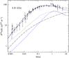 |
Fig. 1 Differential number counts normalized to S5/2 for ERS at 4.8 GHz. Filled squares are observational data (see De Zotti et al. 2010). The plotted curves represent the estimated number counts from the models by Toffolatti et al. (1998, dotted line), De Zotti et al. (2005, blue dash-dotted line), and Massardi et al. (2010, dashed line). Lower curves with the same line types as above represent the estimated number counts of flat-spectrum sources given by the same models. |
In Fig. 2 we plot the differential number counts of these two source populations as calculated from different source samples, which are described in detail in Appendix A. These results require a careful discussion because the simple estimates of source spectral indices are not free from uncertainties, even in the case of negligible errors on published flux densities. First of all, we considered the catalogue of ERS with spectral information based on the NVSS and GB6 surveys (hereafter, the NVSS/GB6 sample), which is defined in Appendix A. Spectral indices from NVSS and GB6 data should be taken with some caution because of the different measurement epoch and the different resolution of the antennae. In particular, biased values of spectral indices could arise for resolution effects, especially when GB6 objects are resolved by the NVSS or have multiple components in the NVSS, which causes a flatter spectral index. On the other hand, variability mostly affects flat-spectrum sources. We discuss this specific problem in Sect. 3.1.
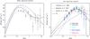 |
Fig. 2 Differential number counts at 4.8 GHz of steep-spectrum (left panel) and flat-spectrum (right panel) ERS from the NVSS/GB6 data (black empty squares). The predictions from the cosmological evolution models plotted in Fig. 1 are represented here by the same line-types as in that figure. In the left panel the thick continuous line represents the difference between the total number counts of the Toffolatti et al. (1998) evolution model and our best fit to the observed number counts of flat-spectrum ERS (right panel; thick continuous line), i.e., it represents our best estimate of the differential number counts of steep-spectrum ERS. In the right panel we also plot the number counts of flat-spectrum ERS estimated from i) NVSS/GB6 data but corrected for resolution effects (black solid squares); ii) the Jackson et al. (2002) sample (red astericks); iii) the CRATES sub-sample in the GB6 sky area (blue empty triangles); iv) the 5-GHz sample of AT20G sources (cyan empty circles). See Sect. 2 for more details. |
For estimating the magnitude of resolution effects on the 4.8-GHz number counts of flat-spectrum sources, we identified all ERS resolved by the NVSS (i.e., with major axis >45 arcsec) that are classified as flat-spectrum sources. We found 173 resolved objects. Because flat-spectrum sources are usually associated with compact objects with an emission dominated by the AGN core, these sources could be false identifications, and we marked them as steep-spectrum sources. Then we dealt with flat-spectrum sources with multiple NVSS counterparts and without clearly dominant NVSS objects: we looked for objects the brightest NVSS counterpart of which contributes <75% of the total flux density and found 102. We redistributed these sources between the two populations according to the proportion of flat- and steep-spectrum sources in flux-density bins. After these corrections, the number counts of flat-spectrum sources were significantly reduced, especially at fluxes S ≲ 300 mJy, whereas at higher fluxes the correction was small (see Fig. 2)5.
Number counts of flat-spectrum sources in Fig. 2 were also obtained from the Parkes quarter-Jy sample (Jackson et al. 2002). The Parkes beam size is 8 arcmin at 2.7 GHz and 4 arcmin at 5 GHz, i.e., a factor 2 larger at the lower frequency. Therefore, resolution effects should go in the opposite direction with respect to the NVSS/GB6 sample. Moreover, we increased the number counts of these sources by 10% (the percentage observed in the NVSS/GB6 sample) to take into account sources with −0.5 ≤ α ≤ −0.4, which were excluded from the original sample.
Figure 2 also shows the results from the CRATES catalogue (Healey et al. 2007) in the area of the GB6 survey. There, the number counts is computed taking into account 8.4-GHz measurements: we calculated the spectral index between 1.4 and 8.4 GHz, and then the differential number counts at 4.8 GHz only for those sources that verified the condition  . The new source counts must be considered a lower limit because some really flat-spectrum sources could have been discarded owing to variability or a spectral steepening between 4.8 and 8.4 GHz. We do not expect many of these, whereas the number of false identifications coming from the classification of NVSS/GB6 data should be strongly reduced. If we compare these number counts with the ones derived from the NVSS/GB6 sample, we see that they partially agree at flux densities S ≳ 0.5 Jy, whereas the discrepancy increases with lower fluxes.
Spectral properties of sources in the NVSS/GB6 sample.
Finally, we also plotted the number counts of flat-spectrum sources estimated from the 5-GHz measurements present in the Australia Telescope Compact Array 20 GHz survey (AT20G; Murphy et al. 2010): we limited our analysis to the almost-complete samples at declination δ < −15° and flux limits 100 mJy and 50 mJy, respectively (indicated as AT20G-d15S100 and AT20G-d15S50, see Appendix A); then, we took all sources with i) measurements at 5 and 8 GHz; ii) 5-GHz flux density S5 ≥ 100 mJy; iii)  . The resulting number counts were corrected for the completeness of the samples and for the percentage of sources with 5- and 8-GHz data (89% and 84% respectively in the two AT20G sub-samples). We observe that the number counts agree well with previous counts at S ≳ 0.5 Jy, and with CRATES data at lower fluxes. ATCA measurements have the advantage to be nearly simultaneous and made with antennae of similar resolutions, which reduces therefore the uncertainty in the spectral index estimates. Although not complete at 5 GHz, the sample built in this way provides reliable results starting from S ≳ 200 mJy, which should be considered at least as a lower limit for fluxes S < 1 Jy.
In Figs. 1, 2 the differential number counts predicted from the cosmological evolution models of Toffolatti et al. (1998), De Zotti et al. (2005), and Massardi et al. (2010) are also displayed. We see that whereas these models fit the total number counts at 5 GHz extremely well, their predictions on the number of flat- or steep-spectrum ERS show significant differences and in general disagree with the published survey data. The Toffolatti et al. (1998) and De Zotti et al. (2005) models fit observational counts of the two populations at flux S > 0.5 Jy quite well, but at lower fluxes they tend to overestimate (in the former case) or to underestimate (in the latter case) the number of flat-spectrum sources. On the other hand, the ratio of steep- and flat-spectrum sources expected from the Massardi et al. (2010) model seems to be quite far from the observed ones, at least for S ≥ 0.1 Jy. It is unlikely that uncertainties in the classification of radio sources could explain this great discrepancy.
As a conclusion, at flux densities S ≥ 100 mJy we can fit the differential number counts of flat-spectrum sources obtained from the observational data by a broken power law  (1)where
  is the differential number counts normalized to S5/2. We find n0 = 47.4 Jy-1sr-1, S0 = 1.67 Jy, k = 0.50 and l = −0.66. We extrapolate this curve also to S < 100 mJy (represented as a thick continuous line in the right panel of Fig. 2).
3. Spectral indices of radio sources
3.1. Spectral index distributions in the NVSS/GB6 sample
It is usually assumed that the spectral index distribution of ERS at GHz frequencies can be described in all flux density ranges by the sum of two Gaussian distributions with maximum at α ~ −0.8 (for steep-spectrum sources) and at α ~ 0.0 (for flat-spectrum sources; see, e.g., De Zotti et al. 2010). For checking this assumption, we calculated the spectral index distributions at 5 GHz of steep- and flat-sources in the NVSS/GB6 sample by dividing them into four flux-density intervals (see Table 1 and Fig. 3). On one hand, the distributions calculated for steep-spectrum sources seem not to change significantly with the flux density, peaking around − 0.9 and having a median spectral index between − 0.81 and − 0.87. On the other hand, the distributions calculated for flat-spectrum sources show a clear dependence on the flux density interval, with steeper spectra at lower flux densities. For S > 400 mJy the maximum in the distribution is around α ~ 0, which agrees well with observations from other surveys (e.g., Ricci et al. 2004). However, at lower flux-density ranges, the maximum in the distributions gradually shifts to lower values of α and is around − 0.4 for S < 251 mJy. The relative number of inverted-spectrum sources (α ≥ 0.3) is about 14% at low flux densities, but it increases to almost 20% at S > 400 mJy.
Variability indices at 1.4 and 4.8 GHz for flat- and steep-spectrum sources.
3.2. Spectral index distributions vs. variability
Because spectral indices are computed from non-simultaneous observations at 1.4 and 4.8 GHz, the source’s variability could affect the spectral index distributions, especially for flat-spectrum sources that are observed to be variable at low frequencies as well. Accordingly, we expect that source variability will induce a higher dispersion in spectral index distributions and, related to it, false identifications between steep- and flat-spectrum source populations.
In Tingay et al. (2003) a study of source variability at GHz frequencies is carried out for 185 sources (167 flat- and 18 steep-spectrum ERS): observations were made over a 3.5 year period with the ATCA at 1.4, 2.5, 4.8 and 8.6 GHz. For each source the authors provide the variability index, defined as the RMS fractional variation from the mean flux density. They found that at 4.8 GHz ~ 40% of flat-spectrum sources show a variability >10%, whereas only 5% vary by >30%. Variability at 1.4 GHz is slightly lower. On the other hand, no significant variability is observed in steep-spectrum sources, except for five sources (over 18) with a variability index between 4 and 20 percent. These results are consistent with variability studies carried out at higher frequencies (Sadler et al. 2006; Bolton et al. 2006).
We assume that flux densities vary at 1.4 and 5 GHz according to the Tingay et al. results, which we summarize in Table 2. We generated a simulated sample of steep- and flat-spectrum sources at 5 GHz with a flux density distribution consistent with the GB6 number counts and with spectral index distributions given by Gaussian functions truncated at α = −0.5 (with peak position αpeak and dispersion σα). The 1.4-GHz flux density is calculated as S5(1.4/5)α. After introducing variability in flux densities at 1.4 and 5 GHz, we computed the new α-distributions by taking into account the uncertainties in GB6 and NVSS flux densities as well. Finally, we found the parameters of the truncated Gaussian distributions (αpeak and σα), for which the simulated α-distributions give the best fits of the observed NVSS/GB6 distributions. The results are reported in Table 1 and in Fig. 3, where we show both the original truncated Gaussians and the final α-distributions produced from them. The value of αpeak is − 0.14 for S ≥ 400 mJy, and steadily decreases to − 0.4 in the lowest flux-density range. We see that simulations can reproduce the NVSS/GB6 results very well. Variability only partially affects the spectral index distributions, increasing their dispersion, and makes some flat-spectrum sources move to the steep-spectrum class. This effect is particularly relevant for sources with spectral index close to −0.5 and at flux densities <250 mJy.
The previous simulations also give us the number of sources that are misclassified because of variability. We found that the number of flat-spectrum sources from the NVSS/GB6 sample can be underestimated by about 5–8 percent, whereas the number of inverted-spectrum sources can be overestimated by only a few percent. Owing to their very low variability, the number of steep-spectrum ERS classified as flat-spectrum sources is small, and only down to S ~ 100 mJy can partially compensate errors in the classification of flat-spectrum ERS.
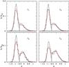 |
Fig. 3 Distributions of the spectral index calculated from the NVSS/GB6 sample for different flux density intervals: i1) S = [100, 158] mJy; i2) S = [158, 251] mJy; i3) S = [251, 400] mJy; i4) S ≥ 400 mJy. The thick black lines are the “best-fit” truncated Gaussians, and the thin red lines are the total distributions obtained from them after introducing source variability (see the text). |
3.3. High-frequency steepening of steep-spectrum sources
A high-frequency spectral steepening is expected in steep-spectrum sources due to electron ageing (Kellermann 1966) and has been observed in multifrequency surveys at ν > 5 GHz (Bolton et al. 2004; Ricci et al. 2006). Ricci et al. (2006) compared the 2.7–5 GHz and 5–18.5 GHz spectral indices and found a median steepening of Δα = 0.32.
A spectral steepening in this frequency range is also observed in the AT20G data: we selected sources in AT20G-d15S50 with 5-GHz flux density S ≥ 500 mJy and spectral index  . We found 211 objects. In Fig. 4 we plot the spectral index distribution computed between 1–5 GHz and 5–20 GHz, and the difference
  . A median steepening of 0.28 is found, in agreement with the Ricci et al. (2006) result. The distribution of Δα is well described by a Gaussian with ⟨ Δα ⟩ = 0.28 and σ ≃ 0.20, except for the negative tail. Values of Δα < 0 (see also the presence of sources with
  in the left panel of Fig. 4) can arise both from sources with spectra that flatten (Tucci et al. 2008) and also from source variability because 1 GHz data are not simultaneous with the AT20G measurements.
At frequencies ν > 20 GHz a further spectral steepening is still possible: a recent indication in this sense is coming from the follow-up of 9C sources (see Waldram et al. 2007).
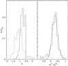 |
Fig. 4 Left panel: distributions of 1–5 GHz (solid line) and 5–20 GHz (dashed line) spectral indices of steep-spectrum sources selected from the AT20G catalogue. Right panel: distribution of the difference |

3.4. High-frequency spectral behaviour of flat-spectrum sources
We focus now on the spectral behaviour of flat-spectrum sources at frequencies ν > 5 GHz. The AT20G survey, thanks to its near-simultaneous observations at 5, 8 and 20 GHz, allows us to study in a quite broad range of frequencies spectral shapes that should be not significantly affected by variability (Massardi et al. 2011a). To this aim, we selected the sources of the AT20G-d15S50 sample with S5 ≥ 200 mJy and with 5–8 GHz spectral index . This sample of 798 objects is about 90% complete for sources with  , but it can lose objects that undergo spectral steepening between 8 and 20 GHz. In Fig. 5 we show the distributions of
  and
and  for those objects. The distribution of is shifted to lower values by about 0.1/0.2 with respect to the distribution, with a large tail of objects with steep spectral index, extending up to − 1.5. The percentage of sources with
  is ~ 22%. The median of distributions, excluding inverted-spectrum (
 ) sources, is − 0.08 and − 0.27 for 5–8 GHz and 8–20 GHz spectral indices, respectively. Figure 5 also shows the histogram of
  . In this case we separate sources with 5–8 GHz spectral indices that are moderately steep (
 ) and flat (
 ). We found that sources with flatter 5–8 GHz spectral index tend to have a more relevant steepening between 8 and 20 GHz (the medians Δα are 0.13 and 0.23, respectively). An interesting feature in both distributions is also the presence of sources with typical steepening around 0.7–0.9, which seem to produce a secondary peak in the Δα distribution of sources with . Because of the incompleteness of the sample for objects with , the peak could be more prominent than observed, and it could extend to Δα ≳ 1. Finally, we note that most inverted-spectrum sources between 5 and 8 GHz () have
  , and only ~ 12% are still inverted up to 20 GHz.
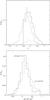 |
Fig. 5 Upper panel: distributions of spectral indices |
Our findings agree well with the results of Massardi et al. (2011a). A very strong average spectral steepening has also been found in the bright PACO sample (Massardi et al. 2011b), where the typical differences between the 5–10 GHz and 30–40 GHz spectral indices are in the range 0.5–1.
Additional indications of a spectral steepening in flat-spectrum sources at frequencies higher than 20 GHz are given by OCRA-p observations at 31 GHz of CRATES selected sources (Peel et al. 2010) and by ATCA observations at 95 GHz of 130 AT20G sources (Sadler et al. 2008). These results are also supported by WMAP data (Gonzalez-Nuevo et al. 2008) at Jy levels, and by ACT data at 148 GHz (Marriage et al. 2011).
4. A spectral model for flat-spectrum sources
As discussed in the previous section, recent multi-frequency surveys have clearly shown that ERS with flat spectra at GHz frequencies can present a downwards spectral curvature already at few tens of GHz. This spectral behaviour could well be an indication that the transition in the synchrotron spectra from the optically-thick to the optically-thin regime is observed, and that this transition can occur even at cm wavelengths. This conclusion is also supported by the results on the compactness of radio sources as a function of the spectral index, obtained from the AT20G survey. As an example, Massardi et al. (2011a, see their Fig. 4) do find a remarkable separation between steep-spectrum () “extended” sources and flat-spectrum ( ) “compact” sources. However, if the compactness is considered versus the spectral index between 8 and 20 GHz, there appears to be also a population of compact and steep-spectrum ERS, corresponding to the 12% of the sample, which is not present at lower frequencies and suggests a spectral steepening at ν < 20 GHz.
By following this hypothesis, the key point for making predictions on the high-frequency contribution of flat-spectrum ERS to number counts is to make an estimate of the frequency at which the spectrum of this source population can experience a substantial steepening (Δα ≳ 0.5). To this aim, we use a simple physical description of the AGN radiation emission in the inner part of their relativistic jets. Our predictions are then calculated on the basis of typical physical parameters in current models for the emission of blazar sources.
4.1. Break frequency in synchrotron spectra from relativistic blazars jets
It is generally believed that flat spectra observed in radio sources result from the superposition of different components of relativistic jets, each with a different synchrotron self-absorption frequency (Kellermann & Pauliny-Toth 1969; Cotton et al. 1980). Relativistic shocks in the jet produce flares that are responsible for radio flux density variations on intervals from months to years (e.g., Marscher & Gear 1985; Valtaoja et al. 1992).
Flat radio spectra are predicted by models of synchrotron emission from inhomogeneous unresolved relativistic jets (Blandford & Königl 1979; Königl 1981). According to them, the observed flux density at a given frequency is dominated by the synchrotron-emitting component, which becomes self-absorbed at that frequency, because synchrotron self-absorption is the most likely absorption mechanism acting in the compact conical jet (Königl 1981). When moving to high frequencies, self-absorbed synchrotron emissions from more and more compact regions are thus observed closer and closer to the AGNs core. However, these models also predict that at a particular frequency, jet emissions cease to be dominated by optically-thick synchrotron emission because of electrons cooling effects, and become dominated by synchrotron emission in optically-thin regime. Spectra then change from “flat” to “steep”.
Let us review in more detail the Königl (1981) model. In this model, the magnetic field H and the distribution of relativistic electrons (described by a power law n(γ) = Kγ − (1 − 2α), where γ is the Lorentz factor) are considered inhomogeneous and scale with the jet radius as H(r) ∝ r − m and K(r) ∝ r − n. We assume m = 1 and n = 2, which corresponds to assuming the magnetic and the electron energy densities are in equipartition (Blandford & Königl 1979).
For the wavelengths range we are interested in, the synchrotron spectra from a portion of a relativistic conical jet at a distance r from the AGN core show two characteristic frequencies:
-
νsm, the frequency where the synchrotron spectrum has the maximum and is estimated by setting the optical depth equal to unity. Below νsm the emitting source is optically thick to synchrotron self-absorption and the flux density rises as ν2.5, whereas at ν > νsm the emission has the optically-thin synchrotron spectrum S ∝ να with α < − 0.5. Under the previous hypothesis, the maximum frequency scales as νsm ∝ r-1. It means that the size of the optically thick “core” of the jet decreases as the observed frequency increases;
-
νsb( > νsm), above which spectra steepen owing to synchrotron-radiation losses (Blandford & Königl 1979). The cutoff occurs when the synchrotron cooling time equals the reacceleration time of electrons. Contrary to νsm, νsb increases as the distance from the core increases, proportionally to r. This implies that in an AGN jet there is a radius rM at which νsm(rM) = νsb(rM). Thus, rM is the smallest radius from which optically-thin synchrotron emission can be observed with its characteristic “steep” spectral index, α < − 0.5.
As said before, the flux density observed from an unresolved conical jet is given by the sum of the emission from the different portions of the jet. The flat part of synchrotron spectra is observed up to the frequency νM (that we call “break frequency”), i.e. the frequency at which νsm(rM) = νsb(rM). At frequencies ν > νM, contributions from regions r < rM inside the jet are negligible owing to the cooling of high-energy electrons. The observed flux density is thus dominated by optically-thin emission from radii r ≥ (ν/νM)rM that verify νsb(r) > ν (Königl 1981).
Therefore, spectra at cm/mm wavelengths can be approximated by two power laws  (2)where αfl and αst represent the effect of the nonuniformity of sources in the optically thick and optically thin regimes.
The frequency νM and the radius rM are provided by Blandford & Königl (1979) and Königl (1981) as the function of the relevant physical quantities of AGN jets. These expressions are quite complex, however, and depend on too many model parameters. For simplicity (and, e.g., in agreement with Marscher 1987; and Ghisellini et al. 1993), we assume that the flux density observed at frequency ≃ νM is dominated only by the emission from the region at radius rM, and that other contributions are negligible. Then, for single emitting regions, synchrotron spectra can be approximately described by the homogeneous spherical model, and the break frequency is given by (Pacholczyk 1970)  (3)where SM is the observed flux density at νM and δ is the Doppler factor. Finally, θ is the observed angular dimension of the emitting region: for a narrow conical jet of semiangle φ, the axis of which makes an angle ψ with the direction of the observer, θ can be written as
 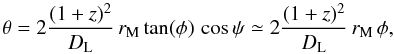 (4)where DL is the luminosity distance of the source, and we assume the view angle ψ ≲ 10° and cosψ ≃ 1. As a typical value, we take φ ~ 0.1 (Königl 1981; Ghisellini & Tavecchio 2009).
Under the hypothesis of equipartition condition, we can also have an estimate of the intensity of the magnetic field in the emitting region. Indeed, from the minimum energy conditions (Pacholczyk 1970), the magnetic field intensity is  (5)where the minimum energy density umin is
  (6)and L is the luminosity of the emitting component, V the volume in pc3. In Eq. (6) we are assuming that the total energy of electrons is equal to the total energy of protons.
In the literature there is no clear agreement on whether the condition of equipartition is valid in blazar jets6. The equipartition magnetic field should be considered only as an upper limit, but because of the weak dependence of νM on H (νM ∝ H1/5), we can safely adopt the equipartition approximation.
The total luminosity in a homogeneous spherical source is related to the break frequency and to the flux density at νM as (the proof is given in Appendix B)  (7)The factor f(α) depends on the optically-thin spectral index and on the lower and upper cutoff in the electron distribution function.
Finally, if the flux density at 5 GHz is known, SM can be extrapolated according to Eq. (2), SM = S5(νM/5)αfl. By substituting in Eq. (3) the equipartition magnetic field Heq calculated above, the break frequency νM then only depends on the physical parameters z, δ and rM, and on the spectral indices before and after the break frequency, νM. Equation (3) thus becomes ![\begin{equation} \nu_{\rm M}\approx C(\alpha,\,\alpha_{\rm fl})\left[D_{\rm L}^{\beta_{\rm D}}(1+z)^{\beta_z}\delta^{\beta_{\delta}} r_{\rm M}^{\beta_r}\right]^{1/\beta}\,, \label{e4b} \end{equation}](/articles/aa/full_html/2011/09/aa16972-11/aa16972-11-eq161.png) (8)with β ≈ 1 + 0.5αfl, βD ≈ 1, βz ≈ − 1.5, βδ ≈ − 0.5 and βr ≈ − 1. The explicit derivation of this equation is given in Appendix B.
(8)with β ≈ 1 + 0.5αfl, βD ≈ 1, βz ≈ − 1.5, βδ ≈ − 0.5 and βr ≈ − 1. The explicit derivation of this equation is given in Appendix B.
4.2. Break frequency and magnetic fields in flat-spectrum sources
The most relevant parameter for the calculation of the break frequency in blazars spectra is, undoubtedly, the radius rM.
The radius rM is the distance from the AGN core of the jet portion that dominates the emission at νM, and it is related to the break frequency approximately as  (in agreement with predictions of inhomogeneous models). This parameter is the most relevant one in the estimate of νM because it defines the dimension and, thus, the compactness of the emitting region at that frequency. At the same time it is also the most critical one, because of the current uncertainty on its real value and of the relatively great range of possible values.
In the radio, i.e. synchrotron, regime the AGN jets emission is expected to be produced at distances along the jet starting from 10-2–10-1 pc up to parsec scales (Marscher 1996; Lobanov 1998; Maraschi & Tavecchio 2003; Lobanov 2010). Moreover, the standard models used to fit the spectral energy distribution (SED) of blazars – i.e. the leptonic homogeneous one-zone model (e.g. Ghisellini et al. 1998; Ghisellini & Tavecchio 2009) – typically find that the “dissipation region” is at a distance from the black hole of around 10-2–10-1 pc (Ghisellini & Tavecchio 2009; Ghisellini et al. 2010). However, the parameters of one-zone models are chosen to fit the high-energy emission of blazars (ν ≳ 1014 Hz), whereas they are not able to reproduce the blazar spectra at cm/mm wavelengths, where the emission is supposed to come from more external and, thus, larger regions of the jet. Therefore, we consider the above quoted values as lower limits for rM. Emission from ultra-compact jet components are also required for explaining observed spectra that keep flat up to frequencies of ≳ 1012 Hz (e.g., Abdo et al. 2010; Gonzalez-Nuevo et al. 2010). On the other hand, observed breaks in blazars spectra at few tens of GHz need higher values of rM. Upper limits for rM are provided by VLBI observations, the resolution of which is of fractions of milliarcseconds at frequencies ν ≲ 5 GHz (see, e.g., Sokolovsky et al. 2011). The typical linear dimensions of the dominant AGN jet components derived from these observations are of the order of a few parsecs (Ghisellini et al. 1993; Jiang et al. 1998; Lobanov 2010).
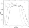 |
Fig. 6 Distribution of the break frequency, νM, for 104 sources with 5-GHz flux density of 1 Jy (solid line), 0.1 Jy (dashed line) and 10 mJy (dotted line). In this plot we only consider 0.01 ≤ rM ≤ 10 pc (case C1). |
To summarize, the range of possible values for rM should be 0.01 ≤ rM ≤ 10 pc (i.e., 3 × 10¹⁶ ≤ rM ≤ 3 × 1019 cm). This is a very large interval and it is taken as a first working case to calculate the break frequency (hereafter, case C1). In addition, we consider more restricted intervals of rM values, distinguishing between FSRQs and BL Lac objects: we take 0.01 ≤ rM ≤ 0.3 pc for BL Lacs and two different cases for FSRQs, 0.03 ≤ rM ≤ 1 pc (hereafter, C2Co, i.e. “more compact”) and 0.3 ≤ rM ≤ 10 pc, a factor of 10 larger (hereafter C2Ex, i.e. “more extended”). rM values are assumed log-uniformly distributed inside the above ranges. This separation in these two classes of blazars is based on the fact that they show different spectral energy distributions SEDs. On one hand, FSRQs, which are more powerful objects, are observed to have a synchrotron peak frequency, νp7, at lower frequencies, around 1012–1014 Hz, without a clear correlation with the radio power. On the other hand, in BL Lacs νp is found to be at higher frequencies and with a larger range of values, from 1013 up to ≳ 1016 Hz (Fossati et al. 1998; Abdo et al. 2010). This difference is motivated by the fact that BL Lacs are characterized by a lower intrinsic power and by a weaker external radiation field. Consequently, in BL Lacs the cooling through radiation losses is less dramatic and the electrons can be present with sufficiently high energies to still mantain synchrotron emission up to these high frequencies (Ghisellini et al. 1998). That is why we assume that BL Lacs are in general more compact objects compared to FSRQs, and that the emitting region at the break frequency, νM, is closer to the AGN core. As a consequence, the break frequency will be found to be on average at higher frequencies in BL Lacs than in FSRQs.
It is important, however, to stress that there is no physical clearly established relationship between the break frequency νM and the peak frequency νp in the synchrotron SED of AGNs. Their relative position can vary a lot from source to source. Indeed, although blazar spectra above νM are dominated by synchrotron emission in the optically-thin regime, the SED of blazars can still continue to increase up to frequencies ≫ νM if the spectral slope is − 1 ≲ α ≲ − 0.5. Interesting examples of SEDs for a complete sample of 104 northern blazars with average fluxes S > 1 Jy at 37 GHz are presented by the Planck Collaboration (2011e), from which it is possible to have an idea of the very different positions of νM and νp in the observed SEDs.
Apart from rM, the other physical quantities relevant for calculating νM from Eq. (8) are the redshift distribution, the Doppler factor δ in AGNs jet, and the spectral indices before and after the break frequency, νM. Values of these physical quantities are discussed in Appendix C and in Sect. 6.
Figures 6, 7 show the distribution of break frequencies in the observer frame for sources with the 5-GHz flux density of S5 = 10, 1, 0.1 and 0.01 Jy, obtained by Eq. (8) for the different choices of rM discussed above. In general, we see that νM is on average lower for fainter sources, as expected from the relation  in Eq. (3). for C1 the large interval of possible values of rM is reflected in an almost flat distribution of the break frequencies in the range 20–1000 GHz, 10–600 GHz, and 2–200 GHz for S5 = 1, 0.1 and 0.01 Jy, respectively. A few percent of sources with break frequency values νM ≳ 1012 Hz are also found. On the other hand, when conditions on rM are stricter, the distributions of νM are narrower. In the cases C2Co-C2Ex we find that most of BL Lacs of 10–1 Jy have a spectral break at ν ≫ 100 GHz, with a significant fraction at ν ≳ 103 GHz. Fainter BL Lacs (100–10 mJy) have νM-distributions peaking around 50–200 GHz. Therefore, according to our results, BL Lacs should be observed at cm/mm wavelengths with almost flat spectra, at least for flux densities > 0.1 Jy. The νM distributions of Jy BL Lacs extend up to 1013 Hz, as does the one for C1.
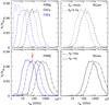 |
Fig. 7 Distribution of the break frequency, νM, for 104 sources with 5-GHz flux density of 10/1/0.1/0.01 Jy (see labels in figure); the rM values correspond to the cases C2Co (black lines) and C2Ex (blue lines). In the two upper panels only model predictions corresponding to the flux densities of 0.01 and 0.1 Jy are shown; in the two lower panels, only predictions corresponding to 1 and 10 Jy are shown. In the lower panel on the left side we also plot the νM (red vertical arrow) of 3C 273 estimated by Clegg et al. (1983). |
For FSRQs, the break frequency varies a lot according to the chosen range of rM: in bright quasars (10–1 Jy), νM is mostly around 102–103 GHz if the emitting regions are more compact and closer to the AGN core (case C2Co), and around 10–100 GHz in the other case (case C2Ex); fainter quasars have νM ≲ 400 GHz in the case C2Co and νM ≲ 40 GHz in the case C2Ex. In general, the two cases give quite different results for the value of νM. For C2Co the majority of Jy and sub-Jy FSRQs can keep flat spectra up to ν ≫ 100 GHz; on the contrary, for C2Ex, apart from the few brightest quasars in the sky, the transition to the optically thin synchrotron spectra can occur already at around 10–20 GHz. As a comparison, we also plot in Fig. 7 the break frequency value, νM = 60 GHz, of 3C 273 estimated by multifrequency quasi-simultaneous observations in Clegg et al. (1983). This value is well within the range expected from the model C2Ex. Additional indications of a break in the spectra of bright blazars around 100 GHz have been reported by analyses of Planck data (Planck Collaboration 2011c,e).
Another physical quantity we can derive from the model is the magnetic field strength in the AGN jet, in equipartition conditions. We plot in Fig. 8 the values of Heq at the jet radius of 1 pc for FSRQ and BL Lac sources with 5-GHz flux densities of S5 = 1, and 0.1 Jy. Magnetic fields in BL Lacs are found to be on average lower than in FSRQs, as expected in less powerful objects. The distributions for Heq are quite sharp, with peak values around 200–1000 mG for FSRQs, and 100–500 mG for BL Lacs. Magnetic field strengths of the order of few hundreds of mG are the values expected using the Königl model in equipartition regime for sources of Jy or sub-Jy flux density (e.g., see results in Jiang et al. 1998; and O’Sullivan & Gabuzda 2009).
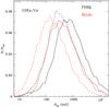 |
Fig. 8 Distribution of the magnetic field strength in equipartition conditions at a distance of 1 pc from the AGN core. Black curves are for FSRQs and red curves for BL Lacs; solid curves are for sources with S5 = 1 Jy and dashed curves if S5 = 0.1 Jy. |
5. High-frequency peaked spectrum sources
The model described in Sect. 4 does not apply to sources with inverted spectra (α ≳ 0.3). Very compact sources have convex spectra, peaking at GHz frequencies (GHz peaked spectrum, GPS, sources) or at tens of GHz (high frequency peakers, HFP). It is now widely agreed that GPS and HFP sources correspond to the early stages of evolution of powerful radio sources when the radio emitting region grows and expands in the interstellar medium of the host galaxy before becoming an extended radio source (see De Zotti et al. 2005, and references therein; O’Dea 1998, for a review). At low luminosity, inverted spectra may also correspond to late stages of AGN evolution, characterized by low radiation/accretion efficiency (De Zotti et al. 2010).
About 5% of sources in the total NVSS/GB6 sample and ~ 15% of flat-spectrum sources have inverted spectra between 1 and 5 GHz; on the other hand, at high flux densities, these fractions increase up to about the 10% and 20% , respectively (see Table 1). The fraction of peaked sources increases significantly in higher frequency surveys. For example, in the AT20G survey, Murphy et al. (2010) found that 21% of sources peak between 5 and 20 GHz, and 14% have a spectrum rising up to 20 GHz (see also Hancock 2009). If we restrict ourselves to the almost-complete subsample AT20G-d15S100, we find about 22% of sources with  , and 18% with , of which about 10% are inverted up to 20 GHz.
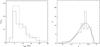 |
Fig. 9 Left panel: distribution of the observed peak frequencies for the sample of inverted-spectrum sources defined in the text (solid line), and for the GPS/HFP candidates in Torniainen et al. (2008). Right panel: distribution of the spectral indexes above the peak frequency for the inverted-spectrum sources. The solid line is given by |
![\hbox{$f(\alpha)=-A(\alpha-\alpha_0)\exp[-0.5(\alpha-\alpha_0)^2/\sigma_{\alpha}^2]$}](/articles/aa/full_html/2011/09/aa16972-11/aa16972-11-eq203.png)
Most of these sources cannot be interpreted as truly young GPS/HFPs, however. Simultaneous multifrequency observations of high-frequency peaked or inverted-spectrum sources have given evidence of high flux-density variability or extended emission in a large number of them, which is not compatible with youth scenario (Dallacasa et al. 2000; Stanghellini 2003; Torniainen et al. 2005; Tinti et al. 2005; Bolton et al. 2006; Orienti et al. 2006; Planck Collaboration 2011d), but indicative that they are most likely blazars caught in an active state, i.e. when a flaring, strongly self-absorbed synchrotron component dominates the emission spectrum. Moreover, when observations are not simultaneous, variability in flat-spectrum sources may lead to misinterpret them as inverted-spectrum sources.
Our approach to this class of sources is purely statistical, without dealing with the physical origin of the emission. We are interested in the spectral shape of inverted-spectrum sources (i.e., all sources with α ≥ 0.3 between 1 and 5 GHz) and in statistically characterizing their behaviour at ν > 5 GHz.
In order to make predictions on the high-frequency number counts, we need some information on the peak frequency (νpeak)8 and on the spectral index above the peak frequency. In the literature we found three samples of sources with simultaneous measurements of a wide frequency range, allowing us to recover this information:
-
Kovalev et al. (1999, hereafter K99) present a nearly simultaneous observation of extragalactic radio sources at six frequencies (0.96, 2.30, 3.90, 7.70, 11.2, and 21.65 GHz) with the RATAN-600 radio telescope. The sample consists of 546 sources selected from the Preston et al. (1985) VLBI survey with a correlated flux density exceeding 0.1 Jy at 2.3 GHz. It includes primarily compact flat-spectrum objects because the Preston et al. sample is complete only for sources with
 .
. -
Dallacasa et al. (2000, hereafter D00) provide a list of 55 high frequency peakers HFPs. This sample was obtained by selecting sources with flux density S5 GHz ≥ 300 mJy and
 from the Green Bank survey 87GB and NVSS. Then HFP
candidates were observed with the VLA at 1.4, 1.7, 4.4, 5, 8, 8.5, 15, and 22.5 GHz,
to acquire simultaneous measurements of radio spectra and to remove variable sources
that do not satisfy the criterion α > 0.5.
from the Green Bank survey 87GB and NVSS. Then HFP
candidates were observed with the VLA at 1.4, 1.7, 4.4, 5, 8, 8.5, 15, and 22.5 GHz,
to acquire simultaneous measurements of radio spectra and to remove variable sources
that do not satisfy the criterion α > 0.5. -
Bolton et al. (2004, hereafter B04) have carried out a follow-up of 176 sources from the 15-GHz 9C survey. Sources were selected from two complete samples with flux limits of 25 and 60 mJy. Simultaneous observations were made at frequencies of 1.4, 4.8, 22, and 43 GHz with the VLA and at 15 GHz with the Ryle Telescope. In addition, 51 sources were also observed at 31 GHz with the OVRO telescope.
Spectra of sources from these three samples were first fitted with a single power law. If the fit was poor, we used a broken power law or a second-order polynomial in logarithmic space. Then we selected all sources with  (where S5 and S1 are the values of the fit at 4.8 and 1.4 GHz). In this way, we created a sample of 142 inverted-spectrum sources: 78 of them come from K99, 50 from D00 and 30 from B04 (16 are in common between K99 and D00). Apart from sources of B04, we were able to estimate the peak frequency only if it occurs at frequencies ν < 20 GHz. We found that most of spectra peak at ν ≲ 10 GHz, and that 117 sources (~80%) have νpeak < 20 GHz. In the B04 sample, where measurements extend up to 43 GHz, there are two objects with 20 < νpeak < 43 GHz and another three that are still inverted at 43 GHz. In Fig. 9 we report the distribution for νpeak up to 20 GHz from our sample and from the GPS/HFP candidates collected by Torniainen et al. (2008): the two distributions agree well. In the plot we considered only the 41 sources in the Torniainen et al. sample classified as “gps” or “convex” and with peak frequency νpeak ≥ 4 GHz. A similar distribution is also given by Vollmer et al. (2008) for a sample of 91 GPS/HFP candidates (see Fig. 7 in that paper).
Results on the distribution of the peak frequency are summarized in Table 3, also for frequencies higher than 20 GHz. We recall that we select only sources with an inverted spectrum between 1 and 5 GHz, and so the distribution is not meaningful for GPS sources with νpeak < 5 GHz. Moreover, in Table 3 we assume that there are no inverted-spectrum sources with peak at frequencies higher than 100 GHz. In any case, current data indicate that the percentage of sources with νpeak > 100 GHz has to be very small and is negligible for our purposes. This hypothesis is supported by the spectral behaviour of sources from simultaneous observations at 20 and 95 GHz by ATCA (Sadler et al. 2008) and by WMAP (Gonzalez-Nuevo et al. 2008). Finally, in simultaneous observations of GPS/HFP candidates by Torniainen et al. (2005, 2007, 2008) the maximum observed peak frequency is ~ 46 GHz, even if their measurements extend up to 250 GHz.
For 98 objects of our sample of inverted-spectrum sources we can provide a reliable estimate of the spectral index after the peak (αhi). The spectral index distribution, plotted in Fig. 9, peaks at αhi ≃ −0.7, but it also has a large tail of steep values up to −2. Similar results were obtained by Snellen et al. (1998). On the other hand, de Vries et al. (1997) found an average αhi ~ −0.7 but no sources with αhi < −1 on a sample of 72 GPS. Since very few data are currently available on this subject, we use the spectral index distribution of Fig. 9 to predict the spectral behaviour of inverted-spectrum sources (α > 0.3) at frequencies above νpeak.
Distribution of the peak frequencies for sources with  .
.
6. Extrapolation of 5-GHz number counts to higher frequencies
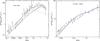 |
Fig. 10 Predicted differential number counts normalized to S-2.5 at 8.44 GHz (left panel) and at 15 GHz (right panel) for the C1 model (thick continuous line), i.e. the model with no difference between the rM value adopted for FSRQs and BL Lac objects (see text). At 8.44 GHz data points are a collection from different samples (see De Zotti et al. 2010), whereas at 15 GHz they have been computed from the 10C survey. In the left panel predictions for number counts of flat- (short-dashed line) and steep-spectrum (dotted line) sources are also shown, compared with results from measurements at 8.4 GHz of flat-spectrum sources by the CRATES program (empty circular points). Predictions at 15 GHz from the De Zotti et al. (2005) model are also shown (blue dash-dotted line). |
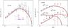 |
Fig. 11 Normalized differential number counts at 20 GHz from AT20G-d15S100 sub-sample of the AT20G survey (filled squares; see text) compared to predictions of the models described in the text: C0(dotted lines), C1 (thick continuous lines), C2Ex (lower red long-dashed lines) and C2Co (upper red long-dashed lines) and the De Zotti et al. (2005) model (blue dash-dotted line). Left panel: the differential number counts for all source populations in the sample. The empty circles are from the 23-GHz WMAP sources catalogue. Right panel: differential number counts for AT20G-d15S100 sources with |


Based on the 5 GHz number counts and on information of spectral properties of ERS described in previous sections, we are now able to make predictions of number counts at cm/mm wavelengths. We deal with the complexity of source spectra as follows.
-
We consider three different populations of radio sources, according to their spectral index in the frequency range 1–5 GHz: steep-spectrum if
; flat-spectrum if  ; inverted-spectrum if . Two flat-spectrum populations are taken into account: FSRQs and BL Lacs.
 -
A simulated source catalogue is produced at 5 GHz. For flat plus inverted-spectrum sources we use the n(S) obtained from the fit of observational data given by Eq. (1). The n(S) of steep-spectrum sources is then extracted as the difference between the total number counts from the Toffolatti et al. (1998) model and the fit of Eq. (1); see also Fig. 2. The fraction of BL Lacs among flat-spectrum sources at 5 GHz, which depends on the flux density, is taken from the evolutionary model of De Zotti et al. (2005). The spectrum for each source is approximated as a power law at ν < 5 GHz. Spectral indices
 are supposed to follow the flux-density dependent spectral index distributions obtained from the NVSS/GB6 sample (see Sect. 3.1 and Table 1).
 -
The 5-GHz flux density of each source is then extrapolated to ν > 5 GHz using the following spectral models.
For steep-spectrum sources we take
 (9)
where
(9)
where  . The spectral steepening Δα is randomly extracted from a Gaussian distribution with average 0.3 and dispersion 0.2, in agreement with the steepening found in the AT20G-d15S50 sample and shown in Fig. 4. A small percentage of flattening or upturning sources is also included.
 For inverted-spectrum sources we use
 (10)where ν0 is directly related to the peak frequency in the spectrum and S0 = (1 − e-1)S(ν0). The coefficients k and l are the spectral indices for the rising and declining parts of the spectrum. We set
  , whereas l is extracted from the best-fit distribution shown in Fig. 9. The peak frequency is extracted from the distribution in Table 3.
 For flat-spectrum sources we use different spectral models. In the simplest one (C0) radio spectra at ν > 5 GHz are modelled as power laws with spectral index
 , where Δα is extracted from Gaussian distributions with
  (11)These values for ⟨ Δα ⟩ (and the associated dispersions) agree with observations from the AT20G survey (see Sect. 3.4).
 As another step in modelling the spectra of flat-spectrum ERS, we introduce a “break frequency”, as discussed in Sect. 4. Spectra are now described by
 (12)where νM is the break frequency, which is interpreted as the frequency at which the transition from the optically thick to the optically thin regime of synchrotron radiation occurs. As above, the spectral index in the optically thick regime at ν > 5 GHz is , with Δα extracted from the Gaussian distributions of Eq. (11), whereas αst is the spectral index in the optically thin regime, determined by synchrotron or IC energy losses, and is taken to be αst = −0.8 ± 0.2, in agreement with Kellermann (1966).
 The break frequency is related to the value of the parameter rM, discussed in Sect. 4.1. We considered three cases:
-
case C1: 0.01 ≤ rM ≤ 10 pc, with no difference between FSRQs and BL Lac objects;
-
case C2Co: 0.01 ≤ rM ≤ 0.3 pc for BL Lacs and 0.03 ≤ rM ≤ 1 pc for FSRQs, i.e. the radio emission in FSRQs arises from a “more compact” region than in the following case, C2Ex;
-
case C2Ex: 0.01 ≤ rM ≤ 0.3 pc, the same value as before for BL Lac objects, and 0.3 ≤ rM ≤ 10 pc for FSRQs, i.e. the radio emission in FSRQs comes from a relatively “more extended” region than in the case C2Co.
-
-
In the end, simulated catalogues can be extracted at differentfrequencies and for different flux limits. Number counts andspectral properties of the three populations of ERS can then becompared with observational data.
7. Predictions on number counts and spectral properties of ERS at ν > 5 GHz
7.1. Number counts: predictions vs observations
A summary of the relevant data is presented in Appendix A. At ν ≲ 30 GHz, we find a general agreement between the observed n(S) and predictions of all models described in the previous section (C0, C1, C2Co or C2Ex). In Fig. 10 we plot our results at 8.4 and 15 GHz, but only for our intermediate model, i.e. C1, because of the very small differences among models. In Fig. 11, thanks to the almost-simultaneous measurements at 5 and 20 GHz for most of the AT20G sources, we test in more detail the goodness of our predictions for the total number counts of sources in the sub-sample AT20G-d15S100 (left panel), as well as for sources within different ranges of  (right panel). Again, all our models are found to agree very well with the data. This is an important confirmation that the adopted number counts at 5 GHz (especially for flat-spectrum sources) and spectral index distributions from the NVSS/GB6 sample are essentially correct.
The agreement with the data is confirmed at 30–33 GHz over a very broad flux density range (Fig. 12), and it extends up to 100 GHz, as shown in Fig. 13.
To distinguish among our models we need data at still higher frequencies (>100 GHz; Fig. 14). The model without a spectral break (C0) overestimates the counts over essentially the whole flux-density range. The other models show the largest differences among each other at the brightest fluxes (at S = 1 Jy, the number counts from the model C2Co are almost a factor 2 higher compared to the model C2Ex), whereas they tend to converge at S < 10 mJy. A very good match with the data is obtained with the model C2Ex, whereas the other models clearly overestimate the Planck counts.
For a direct comparison, we also plot in Fig. 14 the number counts predicted by the De Zotti et al. (2005) cosmological evolution model for ERS. At bright flux densities (S > 0.1 Jy), their results are compatible with our model C0, as expected because both models use simple power-law approximations for blazar spectra. However, at lower fluxes, the differences between these two models increase, and the De Zotti et al. model provides predictions similar to those obtained from our models including a break frequency. This is no surprises because it can be attributed to the different 5-GHz n(S) for flat-spectrum sources that our models use (as shown in Fig. 2), if compared to the De Zotti et al. model9.
Finally, a clear distinction among our models should be provided by the radio source counts at the highest Planck HFI frequencies. Our predictions on integral number counts, N(>S), are presented in Fig. 15 and in Table 4. As an example, the number of objects brighter than 1 Jy should be reduced by ~40% in the range 353–857 GHz for the model C2Ex, but by only ~20% or less in the other cases. Moreover, we predict that the Herschel-ATLAS survey (Eales et al. 2010) will detect from 25 (model C2Ex) to 50 (model C2Co) blazars brighter than 50 mJy at 500 μm over its area of 550 deg2. For comparison, the (De Zotti et al. 2005) model yields ~80 blazars in the same area (Gonzalez-Nuevo et al. 2010).
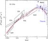 |
Fig. 12 Predicted differential number counts at 33 GHz compared to observational data. The lines have the same meaning as in Fig. 11. The area labelled “GBT” shows estimates by Mason et al. (2009), based on the 31-GHz survey conducted using the GBT and OVRO telescopes. |
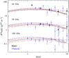 |
Fig. 13 Differential number counts predictions as in Fig. 11 but at 44, 70 and 100 GHz. Bigger black points are from the WMAP NEWPS catalogue by Massardi et al. (2009) at 41 and 61 GHz; smaller blue points are from the Planck ERCSC. For clarity, number counts at 70 GHz are multiplied by 0.1, at 100 GHz by 0.01. |
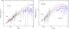 |
Fig. 14 Comparison between predicted and observed differential number counts at 148 GHz (left panel) and at 220 GHz (right panel). Filled circles: ACT data; open black circles: SPT data; open blue circles: Planck ERCSC counts (Planck Collaboration 2011c) at 143 GHz (left panel) and 217 GHz (right panel). The lines have the same meaning as in Fig. 11. |
Number of ERS brighter than 1 and 0.5 Jy in the full sky at the highest Planck frequencies predicted by our models.
7.2. Predicted spectral properties of radio sources
As a further test, we considered the average and the median spectral indices of ERS in catalogues selected at high frequencies. In the ACT sample, all but two of the 42 detections with flux density S148 ≥ 50 mJy have counterparts in AT20G at 5 and 20 GHz (Marriage et al. 2011). An average spectral steepening is found above 20 GHz: the median spectral index and the dispersion of the distribution are  ,
,  and
and  . Somewhat flatter spectral indices are observed for SPT sources (57 objects with a 5-σ detection at 148 and 220 GHz) between 5 and 148 GHz,
  , with a substantial steepening between 148 and 220 GHz,
  (Vieira et al. 2010). To compare these data with model predictions, we produced simulated catalogues of sources selected at 148 GHz with the same flux limits as the SPT and ACT catalogues and with S20 ≥ 50 mJy, and we computed the mean and median spectral indices among pairs of frequencies in the range 5–220 GHz; results are reported in Table 5.
|
Fig. 15 Predictions on integral number counts at 353, 545 and 857 GHz from the models C0, C1, C2Co, C2Ex discussed in Sect. 7. The plotted lines have the same meaning as in Fig. 11. |
Similarly, we used the models to simulate samples selected at 30 GHz with a completeness limit of 1 Jy to compare the predicted median values of spectral indices between 30 GHz and higher Planck frequencies and the associated dispersions with the observed values, given in Table 2 of the Planck Collaboration (2011c). The results are shown in Table 6.
Means, dispersions, and medians of spectral indices calculated between different pairs of frequencies as predicted by our models.
In general, we see that models including a break frequency in blazars spectra are required to explain the median spectral indices ≲ − 0.3 observed when the surveys are performed at frequencies ≥ 100 GHz. In particular, the models C1 and C2Ex yield median spectral indices very similar to the Planck ERCSC ones, i.e.  . They also yield median steepenings
  of 0.14 (C1) and 0.26 (C2Ex) to be compared with 0.32 from ACT data, and
  of 0.22 and 0.28, respectively, to be compared with 0.37 from SPT data (see Table 5). Remarkably, models including a spectral break (at ν ≲ 100 GHz) give quite “flat” mean 5–148 GHz spectral indices (
 ), very close to the value found by Vieira et al. (2010). This is because of the 148 GHz selection that emphasizes sources with flatter spectra.
On the other hand, the median spectral indices yielded by models C0 and C2Co are not compatible with observations at frequencies ≳ 100 GHz.
Predicted median spectral indices of ERS between 30 GHz and the Planck frequency channel indicated in the first row.
8. Conclusions
The main goal of this paper was to present physically grounded models to extrapolate the number counts of ERS, observationally determined over very large flux density intervals at cm wavelengths down to mm wavelengths, where the majority of the experiments aimed at accurately measuring CMB anisotropies are carried out. Accurate extrapolations are necessary to minimize and/or to control the contamination of CMB maps by unresolved extragalactic sources. Moreover, this paper makes a first attempt at constraining the most relevant physical parameters that characterize the emission of blazar sources by using the number counts and the spectral properties of ERS estimated from high-frequency radio surveys.
We focussed on spectra of blazars that dominate the mm-wave number counts of ERS at bright flux densities. In the most recent data sets (e.g., Massardi et al. 2011b; Planck Collaboration 2011c,e), a relevant steepening in blazar spectra with emerging spectral indices in the interval between − 0.5 and − 1.2, is commonly observed. We interpreted this spectral behavior as caused, at least partially, by the transition from the optically-thick to the optically-thin regime in the observed synchrotron emission of AGN jets (see, e.g., Marscher 1996). Indeed, a “break” in the synchrotron spectrum of blazars above which the spectrum becomes “‘steep” is predicted by models of synchrotron emission from inhomogeneous unresolved relativistic jets (Blandford & Königl 1979; Königl 1981; Marscher & Gear 1985). We estimated the value of the frequency νM at which the break occurs on the basis of the ERS flux densities measured at 5 GHz and of the most typical values for the relevant physical parameters of AGNs. In the framework of these models, the most relevant and critical physical parameter is the dimension of the region (approximated as homogeneous and spherical) that is mainly responsible of the emission at the break frequency. For a conical jet model, this parameter can be related to the distance of the emitting region from the AGN core (rM; see Appendix A).
We have investigated four possible cases. The simpler and basic one, C0, assumes simple power-law spectra above 5 GHz, with a dispersion of spectral indices. The other three models feature at high frequencies a spectral break and make different choices for the parameter rM. In model C1 the range of rM (and therefore of νM) is very broad and should include all most likely values expected from theoretical models (see, e.g. Lobanov 2010, for a recent review). Models C2Co and C2Ex assume different distributions of rM for BL Lacs and FSRQs, with the former objects that generate, in general, the synchrotron emission from more compact regions, implying higher values of νM (above 100 GHz for bright objects). These two models differ only in the rM distributions for FSRQs: in the C2Co model the emitting regions are more compact, implying values of νM partially overlapping with those for BL Lacs, whereas in the C2Ex model they are more extended and the values of νM are consequently lower and clearly distinguishable from those adopted for BL Lacs (approximately in the range of 10–300 GHz for S ≳ 1 Jy).
Obviously, high frequency (ν ≥ 100 GHz) data are the most powerful for distinguishing among those models. These data clearly require spectral breaks, thus ruling out model C0, in spite of the average steepening that was introduced in the spectral indices of ERS at ν > 5 GHz, and they favour the model C2Ex. According to this, most of the FSRQs (which are the dominant population at low frequencies and at Jy flux densities), differently from BL Lacs, should bend their flat spectrum before or around 100 GHz. The model also predicts a substantial increase of the BL Lac fraction at high frequencies and bright flux densities. This is indeed observed: a clear dichotomy between FSRQs and BL Lac objects has been found in the Planck ERCSC, where almost all radio sources show very flat spectral indices at LFI frequencies, i.e. αLFI ≳ − 0.2, whereas at HFI frequencies, BL Lacs keep flat spectra, i.e. αHFI ≳ − 0.5, and a high fraction of FSRQs show steeper spectra, i.e. αHFI < − 0.5. Moreover, the fraction of BL Lacs above 1 Jy increases from 10% in the 5-GHz Kühr et al. (1981) sample to 20% in the 37 GHz selected sample discussed by the Planck Collaboration (2011e). More constraints are expected from sub-mm counts of blazars produced by the Herschel surveys (Gonzalez-Nuevo et al. 2010).
According to our model, these results imply that the parameter rM should be of parsec-scales, at least for FSRQs, in agreement with theoretical predictions (Marscher & Gear 1985), whereas values of rM ≪ 1 pc should be only typical of BL Lac objects or of rare quasar sources.
On the other hand, the model C2Ex slightly underestimates the number counts at 20–30 GHz and predicts too steep median spectra at the Planck LFI frequencies. This indicates that spectral breaks at ν < 20 GHz are rarer, i.e. the emitting regions of FSRQs, particularly of the fainter ones, are somewhat more compact than implied by this model. The possibility of more compact AGN cores associated with less powerful sources could agree better with physical models of the AGN jet emission (e.g., Ghisellini et al. 1998), and could provide an improvement of the model predictions at tens of GHz.
The physical model used in this paper adopts only a simplified description of the synchrotron emission in AGN jets and, of course, does not pretend to take into account the complexity of all physical mechanisms involved. Nevertheless, it is capable of providing a clear interpretation of several features observed in blazar spectra. The very interesting quantitative results obtained on number counts and on spectral index distributions of ERS in the whole frequency interval from 5 to 220 GHz clearly support this conclusion. A step forward will be the re-analysis of the luminosity functions of blazar sources at radio frequencies, to follow the cosmological evolution of this class of sources for improving the fit, and the corresponding interpretation of the source number counts at ν > 100 GHz and at faint flux levels. However, this further step will be the subject of a following paper.
Online material
Appendix A: Large-area surveys of radio sources
A.1. Low-frequeny data: the catalogues of steep- and flat-spectrum sources
Large-area deep surveys are specially present at GHz frequencies and have allowed us to make statistical studies of the spectral behaviour of ERS for the basic classification into steep- and flat-spectrum sources.
-
By using the NRAO VLA Sky Survey (NVSS; Condon et al. 1998) at 1.4 GHz and the Green Bank survey (GB6; Gregory et al. 1996) at 4.85 GHz, we built a large and complete catalogue of steep- and flat-spectrum sources at 5 GHz. These two surveys overlap at declinations of 0° < δ < − 75° (i.e., an area Ω ≃ 6.07 sr) and have allowed us to calculate the spectral indices of ERS in almost half of the sky. The resolution of the two surveys is quite different, being 45 arcsec in NVSS and 3.5 arcmin in GB6, whereas the flux limits are 2.5 and 18 mJy respectively. At first, we decided to consider only GB6 sources with flux density S4.85 ≥ 100 mJy and Galactic latitude |b| ≥ 10°. The 100-mJy flux limit for GB6 sources is well above the flux limit of the two surveys and guarantees that we are not losing sources with a rising spectrum, α > 0. Moreover, it minimizes the effects of flux density errors. The Galactic cut at latitude < 10° is to avoid Galactic sources in the sample. In addition, we excluded GB6 sources flagged as “W” (not reliable source) and “C” (confused source). We cross-matched the GB6 source positions with the NVSS catalogue by taking all positive matches within a position offset of 89 arcsec. We used a slightly bigger maximum position offset with respect to Healey et al. (2007) for reducing the number of GB6 sources without NVSS counterparts. In this way, we found 8127 sources with a counterpart in NVSS and only 23 without. Finally, whenever more than one of the NVSS sources fell within the GB6 beam, as a consequence of the better NVSS angular resolution, which may lead to individually resolved multiple components, we summed their fluxes, correcting for the effect of the GB6 beam. We ended up with 2975 flat-spectrum sources (corresponding to ~ 37% of the total number of sources in the sample) and 5152 steep-spectrum sources (~63%). Hereafter, we indicate this source catalogue with spectral information as our NVSS/GB6 sample.
-
The CRATES programme (Healey et al. 2007) has also carried out an almost all-sky sample of flat-spectrum sources brighter than 65 mJy at 5 GHz, using the existing surveys at GHz frequencies. Then they assembled the 8.4-GHz flux densities of flat-spectrum sources from observations done by CLASS (Myers et al. 2003) and from new observations by VLA and ATCA. To mantain uniformity in our analysis, we took into account only CRATES sources in the GB6 area, i.e. where spectra are computed from NVSS and GB6 measurements. In this area, the authors found ~ 5000 flat-spectrum sources with 5-GHz flux density S ≥ 65 mJy (about a 33% of total sources).
-
A sample of flat-spectrum sources is also provided by the Parkes quarter-Jy sample (Jackson et al. 2002; see also De Zotti et al. 2005). It consists of 878 objects selected at 2.7 GHz from several complete surveys of the Parkes radio source catalogue, and having spectral index between 2.7 and 5 GHz
 . The flux limit of these surveys varies between 0.1 and 0.6 Jy, although it is 0.25 Jy for most of them.
A.2. Surveys at frequencies higher than 10 GHz
Recent experiments have surveyed large areas of the sky at frequencies higher than 10 GHz. They are important to test the validity of our predictions on number counts of ERS, but also to provide more direct information on the spectral shape of sources at cm/mm wavelengths.
-
The Ryle-Telescope 9C surveys (Taylor et al. 2001; Waldram et al. 2003) have provided a catalogue of sources at 15 GHz with a completeness limit of 25 mJy. These surveys cover the fields observed by the Very Small Array (VSA), corresponding to an area of ~520 deg2. Moreover, Waldram et al. (2009) have reported on a series of deeper regions, amounting to an area of 115 deg2 complete to approximately 10 mJy, and of 29 deg2 complete to approximately 5.5 mJy. Finally, the Tenth Cambridge (10C) Survey (AMI Consortium 2010) has covered an area of ≈ 27 deg2 at 15.7 GHz down to a completeness limit of 1 mJy (within it, some deeper areas, covering ≈ 12 deg2, are complete down to 0.5 mJy).
-
A 20-GHz survey of the whole southern sky has been carried out by the Australian Telescope Compact Array (ATCA) from 2004 to 2008. The full source catalogue (AT20G) is presented in Murphy et al. (2010) and in Massardi et al. (2011a), and it includes 5890 sources above a flux-density limit of 40 mJy. The completeness of the AT20G catalogue is 93 percent above 100 mJy and 78 percent above 50 mJy in regions south of declination − 15°. Most of sources with declination δ < −15° were also followed-up at 5 and 8 GHz by near-simultaneous observations. In our analysis we made an extensive use of this survey but we limited ourselves to the almost-complete sample of the AT20G catalogue at declinations δ < −15°. It consists of 2195 sources with flux density S ≥ 100 mJy and of 1612 with 50 ≤ S < 100 mJy. We called these two sub-samples AT20G-d15S100 and AT20G-d15S50, if the flux limit is 100 mJy and 50 mJy respectively. For these sources, we were able to determine the spectral index at low frequencies by exploiting ATCA 5-GHz measurements and low-frequency surveys in the southern sky: the NVSS at 1.4 GHz for δ > −40°; the Sydney University Molonglo Sky Survey (SUMSS Mauch at al. 2003) and the Molonglo Galactic Plane Survey (MGPS Murphy et al. 2007) at 843 MHz for δ ≤ −40°. Whereas 5-GHz ATCA measurements were not available, we searched for the source counterparts in the Southern Parkes-MIT-NRAO (PMN) survey (Wright et al. 1994, 1996). In AT20G-d15S100 we obtained the spectral index for 2158 sources, more than 98% of the sub-sample: there were 395 sources with steep spectrum and 1763 with flat spectrum (~82%), of which 471 with inverted spectrum α ≥ 0.3. In Table A.1 we report the number of sources with 5-GHz measurements and the number of steep- and flat-spectrum sources in the two sub-samples of the AT20G. The percentages of flat- and steep-spectrum sources agree with the ones given by Massardi et al. (2011a) over a slightly different and smaller area of AT20G (see their Fig. 1), where they found ~82% and ~74% of flat-spectrum sources with flux density ≥ 100 and 50 mJy respectively.
Table A.1Spectral information in the two almost-complete sub-samples of AT20G.
-
At ν ≃ 30 GHz various CMB experiments have provided samples of extragalactic radio sources, giving estimates of the number counts at different ranges of flux densities: the Cosmic Background Imager (CBI; Mason et al. 2003) in the range 5–50 mJy; the Degree Angular Scale Interferometer (DASI; Kovac et al. 2002) for S ≳ 100 mJy; the Very Small Array (VSA; Cleary et al. 2005) in the range 20–114 mJy; the Sunyaev-Zel’dovich Array (SZA; Muchovej et al. 2010) in the range 0.7–15 mJy.
-
The Wilkinson Microwave Anisotropy Probe (WMAP) carried out all-sky surveys at 23, 33, 41, 61, and 94 GHz and provided a catalogue of ERS at a completeness levels of ≳ 1 Jy. Analyses from the WMAP team have yielded 390 point sources in the five-year data (Wright et al. 2009), whereas 62 new point sources are found in the seven-year data (Gold et al. 2011). WMAP five-year maps has been also analyzed by Massardi et al. (2009) that detected 516 point sources, 457 of which were previously identified as extragalactic sources.
-
Data on ERS are also present for frequencies ν ≳ 100 GHz: the South Pole Telescope (SPT; Vieira et al. 2010) carried out a survey of ERS at 1.4 and 2.0 mm wavelengths with arcmin resolution and mJy depth over an area of 87 deg2; the Atacama Cosmology Telescope (ACT; Marriage et al. 2011) provided a catalog of 157 sources with flux density between 15 and 1500 mJy detected at 148 GHz in an area of 455 deg2.
-
The Planck ERCSC (Planck Collaboration 2011b) reported data on compact sources detected in the nine Planck frequency channels between 30 and 857 GHz during the first 1.6 full-sky surveys. The analysis of the Planck ERCSC data presented in Planck Collaboration (2011c) is limited to a primary sample of 533 compact extragalactic sources at |b| > 5°, selected at 30 GHz. More than the 97% of these compact objects have been identified in external, published catalogues of ERS at GHz frequencies (see the Planck ERCSC Explanatory Supplement, for more details). Moreover, this 30-GHz sample is found to be statistically complete down to a flux density of ≈ 0.9–1.0 Jy and 290 ERS are found at above this flux density limit. The Planck Collaboration has been able to measure the number counts at the Planck LFI (30, 44 and 70 GHz) and at the HFI frequencies of 100, 143 and 217 GHz, with an estimated completeness limits of 1.0, 1.5, 1.1, 0.9, 0.5, 0.4 Jy respectively (Planck Collaboration 2011c).
Appendix B: Estimate of the break frequency in blazars
Spectra for the synchrotron emission from a spherical and homogeneous source have a peak due to the self-absorption of their own radiation. The observed frequency at which the peak of the self-absorption occurs depends on the magnetic field and the depth of the source, and it can be computed by (Pacholczyk 1970) 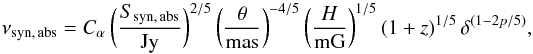 (B.1)where θ is the observed angular dimension of the source and νsyn, abs is measured in GHz. The parameter p depends on the emission model and gives the enhancement of the observed flux due to the beaming (Sobs = δ p − α S). It is equal to 3 for a moving isotropic source and 2 for a continuous jet (see Ghisellini et al. 1993; and Urry & Padovani 1995, for detailed discussion). In the analysis we used as reference value p = 3. We also assumed that emitting electrons have a power-law energy distribution N(γ) = Kγ − (1 − 2α), where α is the spectral index of the optically thin synchrotron emission. The term Cα in Eq. (B.1) depends on α by
 ![\appendix \setcounter{section}{2} \begin{equation} C_{\alpha}=2c_1\Bigg[{4c_6(\alpha) \over \tau_{\rm m}(\alpha)c_5(\alpha)}\Bigg], \end{equation}](/articles/aa/full_html/2011/09/aa16972-11/aa16972-11-eq362.png) (B.2)with c1 = 3e/4πm3c5 and τm the optical depth of the source at νm. The functions c5(α) and c6(α) are provided in Pacholczyk (1970).
(B.2)with c1 = 3e/4πm3c5 and τm the optical depth of the source at νm. The functions c5(α) and c6(α) are provided in Pacholczyk (1970).
As discussed in the text, the break frequency (νM) in a flat-spectrum source is approximately the synchrotron self-absorption frequency νsyn, abs for the innermost part of the jet whose emission is observed at cm/mm wavelengths. If this region is assumed to be homogeneous and spherical (with diameter d), νM can be obtained from Eq. (B.1). For a conical jet geometry, the diameter is related to the distance from the AGN core rM by d = 2rMtan(φ/2) ≃ φrM, where φ is the semiangle of the conical jet.
If the flux density for a flat-spectrum source is known at the observational frequency νo, the observed flux density at νM (SM) can be extrapolated from νo using a power law spectrum (we are assuming that SM ≃ Ssyn, abs, i.e. the contributions from other jet regions are negligible at the frequency νM):  (B.3)Moreover, we have seen from Eq. (5), (6) that the magnetic field in equipartition condition is
 ![\appendix \setcounter{section}{2} \begin{equation} H_{\rm eq}\simeq1.06\times10^{-11}\Bigg[{(L/{\rm Watt}) \over (V/{\rm Kpc}^3)}\Bigg]^{2/7} \,[{\rm mG}]. \end{equation}](/articles/aa/full_html/2011/09/aa16972-11/aa16972-11-eq377.png) (B.4)The total luminosity of the source L can be calculated by the integral of the observed flux density:
(B.4)The total luminosity of the source L can be calculated by the integral of the observed flux density: ![\appendix \setcounter{section}{2} \begin{equation} L=\int_{\nu_{\rm min}}^{\nu_{\rm cut}}L(\nu){\rm d}\nu={4\pi D_{\rm L}^2 \over (1+z)^{1+\alpha}} \delta^{\alpha-p}\int_{\nu_{\rm min}}^{\nu_{\rm cut}}S(\nu){\rm d}\nu~~[{\rm Watt}], \end{equation}](/articles/aa/full_html/2011/09/aa16972-11/aa16972-11-eq379.png) (B.5)where DL is the luminosity distance in Mpc, νmin and νcut give the frequency range where the source emission is concentrated (we take νmin = 10 MHz and νcut = 105 GHz, in agreement with standard assumptions on synchtrotron emission in blazar sources). We used the relation between the luminosity emitted at a given frequency and the observed flux density, which takes into account the K-correction and the relativistic beaming effects on the flux. The integral on the flux density is now expressed as a function of SM and νM:
(B.5)where DL is the luminosity distance in Mpc, νmin and νcut give the frequency range where the source emission is concentrated (we take νmin = 10 MHz and νcut = 105 GHz, in agreement with standard assumptions on synchtrotron emission in blazar sources). We used the relation between the luminosity emitted at a given frequency and the observed flux density, which takes into account the K-correction and the relativistic beaming effects on the flux. The integral on the flux density is now expressed as a function of SM and νM: ![\appendix \setcounter{section}{2} \begin{eqnarray} \int_{\nu_{\rm min}}^{\nu_{\rm cut}}S(\nu){\rm d}\nu & = & \int_{\nu_{\rm min}}^{\nu_{\rm cut}} S_{\rm M}\bigg({\nu \over \nu_{\rm M}}\bigg)^{\alpha}{\rm d}\nu \nonumber \\ & = & {S_{\rm M}\nu_{\rm M}^{-\alpha} \over 1+\alpha}\nu_{\rm cut}^{1+\alpha} \bigg[1-\bigg({\nu_{\rm min} \over \nu_{\rm cut}}\bigg)^{1+\alpha}\bigg] \end{eqnarray}](/articles/aa/full_html/2011/09/aa16972-11/aa16972-11-eq385.png) (B.6)for α ≠ − 1 (if α = −1 the integral is equal to SMνMln(νcut/νmin). Below we assume this condition is verified; it is easy to extend the calculation for α = −1). Using Eq. (B.3) the total luminosity becomes
(B.6)for α ≠ − 1 (if α = −1 the integral is equal to SMνMln(νcut/νmin). Below we assume this condition is verified; it is easy to extend the calculation for α = −1). Using Eq. (B.3) the total luminosity becomes ![\appendix \setcounter{section}{2} \begin{equation} L=C_{\rm L}\,{D_{\rm L}^2\delta^{\alpha-p} \over (1+z)^{1+\alpha}} \nu_{\rm M}^{\alpha_{\rm fl}-\alpha}~~[{\rm Watt}], \end{equation}](/articles/aa/full_html/2011/09/aa16972-11/aa16972-11-eq389.png) (B.7)where
(B.7)where ![\appendix \setcounter{section}{2} \begin{equation} C_{\rm L}\simeq9.5\times10^{27}4\pi S(\nu_o)\nu_o^{-\alpha_{\rm fl}} {\nu_{\rm cut}^{1+\alpha} \over 1+\alpha}\Bigg[1-\bigg({\nu_{\rm min} \over \nu_{\rm cut}}\bigg)^{1+\alpha}\Bigg]. \end{equation}](/articles/aa/full_html/2011/09/aa16972-11/aa16972-11-eq390.png) (B.8)By assuming for simplicity that the source is spherical with diameter d ≃ 0.1rM (Königl 1981; Ghisellini & Tavecchio 2009), we obtain the expression for the magnetic field:
(B.8)By assuming for simplicity that the source is spherical with diameter d ≃ 0.1rM (Königl 1981; Ghisellini & Tavecchio 2009), we obtain the expression for the magnetic field: ![\appendix \setcounter{section}{2} \begin{equation} H=C_H\,{D_{\rm L}^{4/7}\delta^{{2 \over 7}(\alpha-p)} \over (1+z)^{{2 \over 7}(1+\alpha)}} r_{\rm M}^{-6/7}\nu_{\rm M}^{2(\alpha_{\rm fl}-\alpha)/7}~~[{\rm mG}], \label{a3} \end{equation}](/articles/aa/full_html/2011/09/aa16972-11/aa16972-11-eq392.png) (B.9)where
(B.9)where 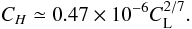 (B.10)The observed angular dimension of the source in Eq. (B.1) is
 ![\appendix \setcounter{section}{2} \begin{equation} \theta=C_{\theta}(1+z^2)r_{\rm M}/D_{\rm L}~~[{\rm mas}], \label{a4} \end{equation}](/articles/aa/full_html/2011/09/aa16972-11/aa16972-11-eq394.png) (B.11)with Cθ ≃ 2.1 × 10⁷.
(B.11)with Cθ ≃ 2.1 × 10⁷.
Finally, including Eqs. (B.3)–(B.11) in Eq. (B.1), the break frequency becomes ![\appendix \setcounter{section}{2} \begin{equation} \nu_{\rm M}=C(\alpha,\,\alpha_{\rm fl})\bigg[D_{\rm L}^{\beta_{\rm D}} (1+z)^{\beta_z} \delta^{\beta_{\delta}}r_{\rm M}^{\beta_d}\bigg]^{1/\beta} , \end{equation}](/articles/aa/full_html/2011/09/aa16972-11/aa16972-11-eq396.png) (B.12)where
(B.12)where 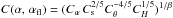 , and
, and 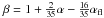 ,
,  ,
,  ,
,  ,
,  .
.
Appendix C: Physical quantities relevant for the estimate of the break frequency in blazars spectra
C.1. Redshift distribution of blazars
In Massardi et al. (2010) the redshift distribution of radio sources at low frequencies is widely discussed, and we followed this paper to derive the redshift distribution of flat-spectrum sources. Most of the samples with redshift information do not distinguish between steep- and flat-spectrum sources. Spectral information are present in the Kühr et al. (1981) catalogue, however: this sample comprises 518 ERS to a 5-GHz flux density limit of 1 Jy, over an area of 9.811 sr. Based on the catalogued spectral indices, 299 sources are classified as flat-spectrum; 212 of which are FSRQs (200 with measured redshift), 26 are BL Lacs (20 with measured redshift) and 61 are classified as galaxies or with missing classification. Moreover, in the Parkes quarter-Jy sample of flat-spectrum ERS (Jackson et al. 2002), redshifts are available for the 58% of sources. From this sample, De Zotti et al. (2005) have defined a complete sub-sample of 514 objects with flux limit of 0.25 Jy, aiming at maximizing the fraction (~75%) of ERS with known redshift. This sub-sample includes 370 FSRQs (93% with known redshift) and 47 BL Lacs, of which only 21% with known redshift.
In Fig. C.1 we plot the redshift distributions of FSRQs and of BL Lacs, and the fits we used for our predictions. For FSRQs only, it has been possible to calculate them from both the samples: in this case, the redshift distribution is observed to shift to higher redshifts as the flux limit of the sample is lowered down, with the peak of the distribution moving from z ≃ 1.2 to z ≃ 1.5. Moreover, Fig. C.1 shows that the relative number of low-redshift FSRQs is strongly reduced, if a fainter flux detection limit is adopted. As for BL Lacs, the redshift distribution can be obtained from the Kühr et al. catalogue, and for only 20 very bright objects. Because of the lack of information at faint fluxes, this redshift distribution will be considered representative also for BL Lac sources with flux density lower than the sample limit. Owing to this, our predictions on number counts of ERS discussed in Sect. 7 are, therefore, more uncertain when applied to sources at S < 0.1 Jy.
 |
Fig. C.1 Upper panels: redshift distributions of BL Lacs (left panel) and of FSRQs (right panel) from the samples by Kühr et al. (1981) (solid points) and Jackson et al. (2002) (empty points), and the corresponding fits (solid and dashed lines, respectively). Lower panels: histograms of the Doppler factor as obtained by Ghisellini et al. (1993) (dashed lines) and Gu et al. (2009) (dotted lines) for BL Lacs (left panel) and core-dominated quasars (right panel). The solid line in the right panel is the fit of the two δ distributions for core-dominated quasars. |
C.2. The Doppler factor in AGNs
The estimate of the Doppler factor δ in AGNs is something complex and model-dependent. In the framework of the synchrotron self-Compton model (Marscher 1987), Ghisellini et al. (1993) calculated the Doppler factor for a sample of 105 radio sources using VLBI measurements of the core angular dimensions and radio fluxes. The value of δ is calculated comparing the observed X-ray fluxes with the ones predicted on the based of a homogeneous spherical emitting model. In Fig. C.1 we show the δ distribution for the 53 core-dominated quasars and the 33 BL Lacs present in the sample. These distributions can be compared with results from Gu et al. (2009) where the Doppler factor is computed using the Königl inhomogeneous jet model instead of the homogeneous spherical model. Their sample consists of 128 sources, with 80 core-dominated quasars and 26 BL Lacs (37 quasars and 19 BL Lacs are in common with the sample used by Ghisellini et al.). The δ distributions are similar in the case of core-dominated quasars, with most of sources having δ between 1 and 30, as expected for objects where the relativistic beamed emission is dominant. For BL Lacs the results from Ghisellini et al. (1993) and Gu et al. (2009) do not agree: the former find very low δ values, extending from 10-2 to 10; in the latter the δ distribution is similar to the core-dominated quasars one. The inhomogeneous model, in general, provides a better description of AGN jet properties, but has the disavantage to involve more free parameters than the homogeneous model. Note, however, that in the case of the homogeneous model it is assumed that all the observed X-ray flux is
produced through inverse Compton scattering by the core component dominanting at the radio frequency. If part of the X-ray flux is produced in other components or by some other mechanism, then the computed δ is a lower limit. For these reasons and for greater simplicity, we assumed the same δ distribution for BL Lacs and core-dominated quasars (in general for all the flat-spectrum sources), described by the fit in Fig. C.1.
Blazar sources are jet-dominated extragalactic objects – observed within a small angle of the jet axis – in which the beamed component dominates the observed emission (Angel & Stockman 1980). They are characterized by a highly variable and polarized non-thermal synchrotron emission at GHz frequencies that is originated from electrons accelerated up to relativistic energies in the collimated jets, which come out of the central active galactic nucleus (AGN; Urry & Padovani 1995).
Various examples of blazar spectra tentatively fitted by different synchrotron components in the AGN jet are also given by Planck Collaboration (2011e).
Recently, Very Long Baseline Array (VLBA) simultaneous observations of the frequency-dependent shift seen in the core position of blazar sources (known as the “core shift”) at nine frequencies in the 1.4–15.4 GHz range (Sokolovsky et al. 2011) have found new evidence of a parameter value k ≈ 1 in the above quoted law, confirming theoretical predictions.
According to Maraschi & Tavecchio (2003), the condition is verified in flat-spectrum quasars, but not in BL Lacs, where the magnetic field energy is observed to be lower than the relativistic particle energy. Indications that the brightness temperature of the radio emission in jet components rapidly drops to the equipartition limit moving away from the core are also given by Lobanov (2010) and references therein. On the other hand, Ghisellini et al. (2010) argue that blazar jets should be matter-dominated on scales where most of their luminosity is produced, and sub-equipartition magnetic fields are found only on smaller scales.
Acknowledgments
M.T. would like to thank Monica Orienti for the useful and enlightening discussions about the main physical mechanisms in AGNs. M.T. thanks the Physikalisch-Meteorologisches Observatorium Davos/World Radiation Center (PMOD/WRC) for having provided him with facilities to carry out the present research. L.T. and E.M.G. acknowledge partial financial support from the Spanish Ministry of Education and Science (MEC), under project AYA2007-68058-C03-02, and from the Spanish Ministry of Science and Innovation (MICINN), under project AYA2010-21766-C03-01. GDZ acknowledges financial support from ASI (ASI/INAF Agreement I/072/09/0 for the Planck LFI activity of Phase E2).
References
- Abdo, A. A., Ackermann, M., & Ajello, M. 2010, ApJ, 716, 30 [NASA ADS] [CrossRef] [Google Scholar]
- AMI Consortium: Davies, M. L., Franzen, T. M. O., Waldram, E. M., et al. 2010, MNRAS, submitted [arXiv:1012.3659] [Google Scholar]
- Angel, J. R. P., & Stockman, H. S. 1980, Ann. Rev. Astron. Astrophys., 18, 321 [Google Scholar]
- Bennett, C. L., Hill, R. S., Hinshaw, G., et al. 2003, ApJS, 148, 97 [NASA ADS] [CrossRef] [Google Scholar]
- Blandford, R. D., & Königl, A. 1979, ApJ, 232, 34 [NASA ADS] [CrossRef] [Google Scholar]
- Bolton, R. C., Cotter, G., Pooley, G. G., et al. 2004, MNRAS, 354, 485 [NASA ADS] [CrossRef] [Google Scholar]
- Bolton, R. C., Chandler, C. J., Cotter, G., et al. 2006, MNRAS, 370, 1556 [NASA ADS] [CrossRef] [Google Scholar]
- Cleary, K. A., Taylor, A. C., Waldram, E., et al. 2005, MNRAS, 360, 340 [NASA ADS] [CrossRef] [Google Scholar]
- Clegg, P. E., Gear, W. K., Ade, P. A. R., et al. 1983, ApJ, 273, 58 [NASA ADS] [CrossRef] [Google Scholar]
- Condon, J. J., Cotton, W. D., Greisen, E. W., et al. 1998, AJ, 115, 1693 [NASA ADS] [CrossRef] [Google Scholar]
- Cotton, W. D., Wittels, J. J., & Shapiro, I. I. 1980, ApJL, 238, L123 [NASA ADS] [CrossRef] [Google Scholar]
- Dallacasa, D., Stanghellini, C., Centonza, M., & Fanti, R. 2000, A&A, 363, 887 [NASA ADS] [Google Scholar]
- Danese, L., Franceschini, A., Toffolatti, L., & De Zotti, G. 1987, ApJ, 318, L15 [NASA ADS] [CrossRef] [Google Scholar]
- De Zotti, G., Ricci, R., Mesa, D., et al. 2005, A&A, 431, 893 [NASA ADS] [CrossRef] [EDP Sciences] [Google Scholar]
- De Zotti, G., Massardi, M., Negrello, M., & Wall, J. 2010, A&AR, 18, 1 [Google Scholar]
- de Vries, W. H., Barthel, P. D., & O’Dea, C. P. 1997, A&A, 321, 105 [NASA ADS] [Google Scholar]
- Dunlop, J. S., & Peacock, J. A. 1990, MNRAS, 247, 19 [NASA ADS] [Google Scholar]
- Eales, S., Dunne, L., Clements, D., et al. 2010, PASP, 122, 499 [NASA ADS] [CrossRef] [Google Scholar]
- Fossati, G., Maraschi, L., Celotti, A., Comastri, A., & Ghisellini, G. 1998, MNRAS, 299, 433 [NASA ADS] [CrossRef] [Google Scholar]
- Ghisellini, G. 2010 [arXiv:1002.4619] [Google Scholar]
- Ghisellini, G., & Tavecchio, F. 2009, MNRAS, 397, 985 [NASA ADS] [CrossRef] [Google Scholar]
- Ghisellini, G., Maraschi, L., & Treves, A. 1985, A&A, 146, 204 [NASA ADS] [Google Scholar]
- Ghisellini, G., Padovani, P., Celotti, A., & Maraschi, L. 1993, ApJ, 407, 65 [Google Scholar]
- Ghisellini, G., Celotti, A., Fossati, G., Maraschi, L., & Comastri, A. 1998, MNRAS, 301, 451 [NASA ADS] [CrossRef] [Google Scholar]
- Ghisellini, G., Tavecchio, F., Foschini, L., et al. 2010, MNRAS, 402, 497 [NASA ADS] [CrossRef] [Google Scholar]
- Giommi, P., & Colafrancesco, S. 2004, A&A, 414, 7 [NASA ADS] [CrossRef] [EDP Sciences] [Google Scholar]
- Gold, B., Odegard, N., Weiland, J. L., et al. 2011, ApJS, 192, 15 [Google Scholar]
- Gonzalez-Nuevo, J., Massardi, M., Argüeso, F., et al. 2008, MNRAS, 384, 711 [NASA ADS] [CrossRef] [Google Scholar]
- Gonzalez-Nuevo, J., de Zotti, G., Andreani, P., et al. 2010, A&A, 518, L38 [NASA ADS] [CrossRef] [EDP Sciences] [Google Scholar]
- Gregory, P. C., Scott, W. K., Douglas, K., & Condon, J. J. 1996, ApJS, 103, 427 [NASA ADS] [CrossRef] [Google Scholar]
- Gu, M., Cao, X., & Jiang, D. R. 2009, MNRAS, 396, 984 [NASA ADS] [CrossRef] [Google Scholar]
- Hancock, P. J. 2009, AN, 330, 180 [NASA ADS] [Google Scholar]
- Healey, S. E., Romani, R. W., Gregory, B. T., et al. 2007, ApJS, 171, 61 [NASA ADS] [CrossRef] [Google Scholar]
- Jackson, C. A., & Wall, J. V. 1999, 304, 160 [Google Scholar]
- Jackson, C. A., Wall, J. V., & Shaver, P. A. 2002, A&A, 386, 97 [NASA ADS] [CrossRef] [EDP Sciences] [Google Scholar]
- Jiang, D. R., Cao, X., & Hong, X. 1998, ApJ, 494, 139 [NASA ADS] [CrossRef] [Google Scholar]
- Kellermann, K. I. 1966, ApJ, 146, 621 [NASA ADS] [CrossRef] [Google Scholar]
- Kellermann, K. I., & Pauliny-Toth, I. I. K. 1969, ApJ, 155, L71 [NASA ADS] [CrossRef] [Google Scholar]
- Königl, A. 1981, ApJ, 243, 700 [NASA ADS] [CrossRef] [Google Scholar]
- Kovac, J. M., Leitch, E. M., Pryke, C., et al. 2002, Nature, 420, 772 [NASA ADS] [CrossRef] [PubMed] [Google Scholar]
- Kovalev, Y. Y., Nizhelsky, N. A., Kovalev, Y. A., et al. 1999, A&AS, 139, 545 [NASA ADS] [CrossRef] [EDP Sciences] [Google Scholar]
- Kühr, H., Witzel, A., Pauliny-Toth, I. I. K., & Nauber, U. 1981, A&AS, 45, 367 [NASA ADS] [Google Scholar]
- Lobanov, A. P. 1998, A&A, 330, 79 [NASA ADS] [Google Scholar]
- Lobanov, A. P. 2010 [arXiv:1010.2856] [Google Scholar]
- Maraschi, L., & Tavecchio, F. 2003, ApJ, 593, 667 [NASA ADS] [CrossRef] [Google Scholar]
- Marecki, A., Falcke, H., Niezgoda, J., Garrington, S. T., & Patnaik, A. R. 1999, A&ASS, 135, 273 [NASA ADS] [CrossRef] [EDP Sciences] [Google Scholar]
- Marriage, T. A., Juin, J. B., Lin, Y.-T., et al. 2011, ApJ, 731, 100 [Google Scholar]
- Marscher, A. P. 1980a, Nature, 286, 12 [NASA ADS] [CrossRef] [PubMed] [Google Scholar]
- Marscher, A. P. 1980b, ApJ, 235, 86 [Google Scholar]
- Marscher, A. P. 1987, in Superluminal Radio Sources, ed. J. A. Zensus, & T. J. Pearson (Cambridge: Cambridge Univ. Press), 280 [Google Scholar]
- Marscher, A. P. 1996, in Energy transport in radio galaxies and quasars, ed. P. E. Hardee, A. H. Bridle, & J. A. Zensus (San Francisco: ASP), ASP Conf. Ser., 100, 45 [Google Scholar]
- Marscher, A. P., & Gear, W. K. 1985, ApJ, 298, 114 [NASA ADS] [CrossRef] [Google Scholar]
- Mason, B. S., Pearson, T. J., & Readhead, A. C. S. 2003, ApJ, 591, 540 [Google Scholar]
- Mason, B. S., Weintraub, L., & Sievers, J. 2009, ApJ, 704, 1433 [NASA ADS] [CrossRef] [Google Scholar]
- Massardi, M., Ekers, R. D., Murphy, T., et al. 2008, MNRAS, 384, 775 [NASA ADS] [CrossRef] [Google Scholar]
- Massardi, M., Lopez-Caniego, M., Gonzalez-Nuevo, J., et al. 2009, MNRAS, 392, 733 [NASA ADS] [CrossRef] [Google Scholar]
- Massardi, M., Bonaldi, A., Negrello, M., et al. 2010, MNRAS, 404, 532 [NASA ADS] [Google Scholar]
- Massardi, M., Ekers, R. D., Murphy, T., et al. 2011a, MNRAS, 412, 318 [NASA ADS] [CrossRef] [Google Scholar]
- Massardi, M., Bonaldi, A., Bonavera, L., et al. 2011b, MNRAS, in press [arXiv:1101.0225] [Google Scholar]
- Mauch, T., Murphy, T., Buttery, H. J., et al. 2003, MNRAS, 342, 1117 [NASA ADS] [CrossRef] [Google Scholar]
- Muchovej, S., Leitch, E., Carlstrom, J. E., et al. 2010, ApJ, 716, 521 [NASA ADS] [CrossRef] [Google Scholar]
- Murphy, T., Mauch, T., Green, A., et al. 2007, MNRAS, 382, 382 [NASA ADS] [CrossRef] [Google Scholar]
- Murphy, T., Sadler, E. M., Ekers, R. D., et al. 2010, MNRAS, 402, 2403 [NASA ADS] [CrossRef] [Google Scholar]
- Myers, S. T., Jackson, N. J., Browne, I. W. A., et al. 2003, MNRAS, 341, 1 [NASA ADS] [CrossRef] [Google Scholar]
- O’Dea, C. P. 1998, PASP, 110, 493 [NASA ADS] [CrossRef] [Google Scholar]
- Orienti, M., Dallacasa, D., Tinti, S., & Stanghellini, C. 2006, A&A, 450, 959 [NASA ADS] [CrossRef] [EDP Sciences] [Google Scholar]
- O’Sullivan, S. P., & Gabuzda, D. C. 2009, MNRAS, 400, 26 [NASA ADS] [CrossRef] [Google Scholar]
- Pacholczyk, A. G. 1970, Radio Astrophysics, Series of Books in A&A (San Francisco: Freeman) [Google Scholar]
- Peel, M. W., Gawronski, M. P., Battye, R. A., et al. 2011, MNRAS, 410, 2690 [NASA ADS] [CrossRef] [Google Scholar]
- Planck Collaboration. 2011a, Planck early results 01: The Planck Mission, A&A, in press, DOI: 10.1051/0004-6361/201116464 [arXiv:1101.2022] [Google Scholar]
- Planck Collaboration 2011b, Planck early results 07: The Early Release Compact Source Catalogue, A&A, in press, DOI: 10.1051/0004-6361/201116474 [arXiv:1101.2041] [Google Scholar]
- Planck Collaboration 2011c, Planck early results 13: Statistical properties of extragalactic radio sources in the Planck Early Release Compact Source Catalogue, A&A, in press, DOI: 10.1051/0004-6361/201116471 [arXiv:1101.2044v2] [Google Scholar]
- Planck Collaboration 2011d, Planck early results 14: Early Release Compact Source Catalogue validation and extreme radio sources, A&A, in press, DOI: 10.1051/0004-6361/201116475 [arXiv:1101.1721v2] [Google Scholar]
- Planck Collaboration 2011e, Planck early results 15: Spectral energy distributions and radio continuum spectra of northern extragalactic radio sources, A&A, in press, DOI: 10.1051/0004-6361/201116466 [arXiv:1101.2047] [Google Scholar]
- Preston, R. A., Morabito, D. D., Williams, J. G., et al. 1985, AJ, 90, 1599 [NASA ADS] [CrossRef] [Google Scholar]
- Ricci, R., Sadler, E. M., Ekers, R. D., et al. 2004, MNRAS, 354, 305 [NASA ADS] [CrossRef] [Google Scholar]
- Ricci, R., Prandoni, I., Grupponi, C., Sault, R. J., & De Zotti, G. 2006, A&A, 445, 465 [NASA ADS] [CrossRef] [EDP Sciences] [Google Scholar]
- Sadler, E. M., Ricci, R., Ekers, R. D., et al. 2006, MNRAS, 371, 898 [NASA ADS] [CrossRef] [Google Scholar]
- Sadler, E. M., Ricci, R., Ekers, R. D., et al. 2008, MNRAS, 385, 1656 [NASA ADS] [CrossRef] [Google Scholar]
- Ricci, R., Prandoni, I., Grupponi, C., Sault, R. J., & De Zotti, G. 2006, A&A, 445, 465 [NASA ADS] [CrossRef] [EDP Sciences] [Google Scholar]
- Snellen, I. A. G., Schilizzi, R. T., de Bruyn, A. G., et al. 1998, A&A, 131, 435 [Google Scholar]
- Sokolovsky, K. V., Kovalev, Y. Y., Pushkarev, A. B., & Lobanov, A. P. 2011, A&A, 532, A38 [NASA ADS] [CrossRef] [EDP Sciences] [Google Scholar]
- Stanghellini, C. 2003, PASA, 20, 118 [NASA ADS] [Google Scholar]
- Tauber, J. A., Mandolesi, N., Puget, J.-L., et al. 2010, A&A, 520, A1 [NASA ADS] [CrossRef] [EDP Sciences] [Google Scholar]
- Taylor, A. C., Grainge, K. J. B., Jones, M. E., et al. 2001, MNRAS, 327, L1 [NASA ADS] [CrossRef] [Google Scholar]
- Tingay, S. J., Jauncey, D. L., King, E. A., et al. 2003, PASJ, 55, 351 [NASA ADS] [Google Scholar]
- Tinti, S., Dallacasa, D., De Zotti, G., Celotti, A., & Stanghellini, C. 2005, A&A, 432, 31 [NASA ADS] [CrossRef] [EDP Sciences] [Google Scholar]
- Toffolatti, L., Franceschini, A., De Zotti, G., et al. 1987, A&A, 184, 7 [NASA ADS] [Google Scholar]
- Toffolatti, L., Argüeso, F., De Zotti, G., et al. 1998, MNRAS, 297, 117 [NASA ADS] [CrossRef] [Google Scholar]
- Toffolatti, L., Argüeso, F., De Zotti, G., & Burigana, C. 1999, Microwave Foregrounds, ed. A. de Oliveira-Costa, & M. Tegmark (San Francisco: ASP), ASP Conf. Ser., 181, 153 [Google Scholar]
- Toffolatti, L., Negrello, M., González-Nuevo, J., et al. 2005, A&A, 438, 475 [NASA ADS] [CrossRef] [EDP Sciences] [Google Scholar]
- Torniainen, I., Tornikoski, M., Teräsranta, H., Aller, M. F., & Aller, H. D. 2005, A&A, 435, 839 [NASA ADS] [CrossRef] [EDP Sciences] [Google Scholar]
- Torniainen, I., Tornikoski, M., Lähteenmäki A., et al. 2007, A&A, 469, 451 [NASA ADS] [CrossRef] [EDP Sciences] [Google Scholar]
- Torniainen, I., Tornikoski, M., Turunen, M., et al. 2008, A&A, 482, 483 [NASA ADS] [CrossRef] [EDP Sciences] [Google Scholar]
- Tucci, M., Martínez-González, E., Toffolatti, L., González-Nuevo, J., & De Zotti, G. 2004, MNRAS, 349, 1267 [NASA ADS] [CrossRef] [Google Scholar]
- Tucci, M., Martínez-González, E., Vielva, P., & Delabrouille, J. 2005, MNRAS, 360, 935 [NASA ADS] [CrossRef] [Google Scholar]
- Tucci, M., Rubiño-Martin, J. A., Rebolo, R., et al. 2008, MNRAS, 386, 1729 [NASA ADS] [CrossRef] [Google Scholar]
- Unwin S. C., Wehrle, A. E., Urry, C. M., et al. 1994, ApJ, 432, 103 [NASA ADS] [CrossRef] [Google Scholar]
- Urry, C. M., & Padovani, P. 1995, PASP, 107, 803 [NASA ADS] [CrossRef] [Google Scholar]
- Valtaoja, E., Teräsranta, H., Urpo, S., et al. 1992, A&A, 254, 71 [NASA ADS] [Google Scholar]
- Vielva, P., Martinez-Gonzalez, E., Cayon, L., et al. 2001, MNRAS, 326, 181 [NASA ADS] [CrossRef] [Google Scholar]
- Vielva, P., Martinez-Gonzalez, E., Gallegos, J. E., Toffolatti, L., & Sanz, J. L. 2003, MNRAS, 344, 89 [NASA ADS] [CrossRef] [Google Scholar]
- Vieira, J. D., Crawford, T. M., Switzer, E. R., et al. 2010, ApJ, 719, 763 [NASA ADS] [CrossRef] [Google Scholar]
- Vollmer, B., Krichbaum, T. P., Angelakis, E., & Kovalev, Y. Y. 2008, A&A, 489, 49 [NASA ADS] [CrossRef] [EDP Sciences] [Google Scholar]
- Waldram, E. M., Pooley, G. G., Grainge, K. J. B., et al. 2003, MNRAS, 342, 915 [NASA ADS] [CrossRef] [Google Scholar]
- Waldram, E. M., Bolton, R. C., Pooley, G. G., & Riley, J. M. 2007, MNRAS, 379, 1442 [NASA ADS] [CrossRef] [Google Scholar]
- Waldram, E. M., Pooley, G. G., Davies, M. L., Grainge, K. J. B., & Scott, P. F. 2009, MNRAS, submitted [arXiv:0908.0066] [Google Scholar]
- Watson, R. A., Carreira, P., Cleary, K., et al. 2003, MNRAS, 341, 1057 [NASA ADS] [CrossRef] [Google Scholar]
- Wright, A. E., Griffith, M. R., Burke, B. F., & Ekers, R. D. 1994, ApJS, 91, 111 [NASA ADS] [CrossRef] [Google Scholar]
- Wright, A. E., Griffith, M. R., Hunt, A. J., et al. 1996, ApJS, 103, 145 [NASA ADS] [CrossRef] [Google Scholar]
- Wright, E. L., Chen, X., Odegard, N., et al. 2009, ApJS, 180, 283 [NASA ADS] [CrossRef] [Google Scholar]
- Zensus, J. A., Cohen, M. H., & Unwin, S. C. 1995, ApJ, 443, 35 [NASA ADS] [CrossRef] [Google Scholar]
All Tables
Number of ERS brighter than 1 and 0.5 Jy in the full sky at the highest Planck frequencies predicted by our models.
Means, dispersions, and medians of spectral indices calculated between different pairs of frequencies as predicted by our models.
Predicted median spectral indices of ERS between 30 GHz and the Planck frequency channel indicated in the first row.
All Figures
|
Fig. 1 Differential number counts normalized to S5/2 for ERS at 4.8 GHz. Filled squares are observational data (see De Zotti et al. 2010). The plotted curves represent the estimated number counts from the models by Toffolatti et al. (1998, dotted line), De Zotti et al. (2005, blue dash-dotted line), and Massardi et al. (2010, dashed line). Lower curves with the same line types as above represent the estimated number counts of flat-spectrum sources given by the same models. |
| In the text | |
|
Fig. 2 Differential number counts at 4.8 GHz of steep-spectrum (left panel) and flat-spectrum (right panel) ERS from the NVSS/GB6 data (black empty squares). The predictions from the cosmological evolution models plotted in Fig. 1 are represented here by the same line-types as in that figure. In the left panel the thick continuous line represents the difference between the total number counts of the Toffolatti et al. (1998) evolution model and our best fit to the observed number counts of flat-spectrum ERS (right panel; thick continuous line), i.e., it represents our best estimate of the differential number counts of steep-spectrum ERS. In the right panel we also plot the number counts of flat-spectrum ERS estimated from i) NVSS/GB6 data but corrected for resolution effects (black solid squares); ii) the Jackson et al. (2002) sample (red astericks); iii) the CRATES sub-sample in the GB6 sky area (blue empty triangles); iv) the 5-GHz sample of AT20G sources (cyan empty circles). See Sect. 2 for more details. |
| In the text | |
|
Fig. 3 Distributions of the spectral index calculated from the NVSS/GB6 sample for different flux density intervals: i1) S = [100, 158] mJy; i2) S = [158, 251] mJy; i3) S = [251, 400] mJy; i4) S ≥ 400 mJy. The thick black lines are the “best-fit” truncated Gaussians, and the thin red lines are the total distributions obtained from them after introducing source variability (see the text). |
| In the text | |
|
Fig. 4 Left panel: distributions of 1–5 GHz (solid line) and 5–20 GHz (dashed line) spectral indices of steep-spectrum sources selected from the AT20G catalogue. Right panel: distribution of the difference |
| In the text | |
|
Fig. 5 Upper panel: distributions of spectral indices |
| In the text | |
|
Fig. 6 Distribution of the break frequency, νM, for 104 sources with 5-GHz flux density of 1 Jy (solid line), 0.1 Jy (dashed line) and 10 mJy (dotted line). In this plot we only consider 0.01 ≤ rM ≤ 10 pc (case C1). |
| In the text | |
|
Fig. 7 Distribution of the break frequency, νM, for 104 sources with 5-GHz flux density of 10/1/0.1/0.01 Jy (see labels in figure); the rM values correspond to the cases C2Co (black lines) and C2Ex (blue lines). In the two upper panels only model predictions corresponding to the flux densities of 0.01 and 0.1 Jy are shown; in the two lower panels, only predictions corresponding to 1 and 10 Jy are shown. In the lower panel on the left side we also plot the νM (red vertical arrow) of 3C 273 estimated by Clegg et al. (1983). |
| In the text | |
|
Fig. 8 Distribution of the magnetic field strength in equipartition conditions at a distance of 1 pc from the AGN core. Black curves are for FSRQs and red curves for BL Lacs; solid curves are for sources with S5 = 1 Jy and dashed curves if S5 = 0.1 Jy. |
| In the text | |
|
Fig. 9 Left panel: distribution of the observed peak frequencies for the sample of inverted-spectrum sources defined in the text (solid line), and for the GPS/HFP candidates in Torniainen et al. (2008). Right panel: distribution of the spectral indexes above the peak frequency for the inverted-spectrum sources. The solid line is given by |
| In the text | |
|
Fig. 10 Predicted differential number counts normalized to S-2.5 at 8.44 GHz (left panel) and at 15 GHz (right panel) for the C1 model (thick continuous line), i.e. the model with no difference between the rM value adopted for FSRQs and BL Lac objects (see text). At 8.44 GHz data points are a collection from different samples (see De Zotti et al. 2010), whereas at 15 GHz they have been computed from the 10C survey. In the left panel predictions for number counts of flat- (short-dashed line) and steep-spectrum (dotted line) sources are also shown, compared with results from measurements at 8.4 GHz of flat-spectrum sources by the CRATES program (empty circular points). Predictions at 15 GHz from the De Zotti et al. (2005) model are also shown (blue dash-dotted line). |
| In the text | |
|
Fig. 11 Normalized differential number counts at 20 GHz from AT20G-d15S100 sub-sample of the AT20G survey (filled squares; see text) compared to predictions of the models described in the text: C0(dotted lines), C1 (thick continuous lines), C2Ex (lower red long-dashed lines) and C2Co (upper red long-dashed lines) and the De Zotti et al. (2005) model (blue dash-dotted line). Left panel: the differential number counts for all source populations in the sample. The empty circles are from the 23-GHz WMAP sources catalogue. Right panel: differential number counts for AT20G-d15S100 sources with |
| In the text | |
|
Fig. 12 Predicted differential number counts at 33 GHz compared to observational data. The lines have the same meaning as in Fig. 11. The area labelled “GBT” shows estimates by Mason et al. (2009), based on the 31-GHz survey conducted using the GBT and OVRO telescopes. |
| In the text | |
|
Fig. 13 Differential number counts predictions as in Fig. 11 but at 44, 70 and 100 GHz. Bigger black points are from the WMAP NEWPS catalogue by Massardi et al. (2009) at 41 and 61 GHz; smaller blue points are from the Planck ERCSC. For clarity, number counts at 70 GHz are multiplied by 0.1, at 100 GHz by 0.01. |
| In the text | |
|
Fig. 14 Comparison between predicted and observed differential number counts at 148 GHz (left panel) and at 220 GHz (right panel). Filled circles: ACT data; open black circles: SPT data; open blue circles: Planck ERCSC counts (Planck Collaboration 2011c) at 143 GHz (left panel) and 217 GHz (right panel). The lines have the same meaning as in Fig. 11. |
| In the text | |
|
Fig. 15 Predictions on integral number counts at 353, 545 and 857 GHz from the models C0, C1, C2Co, C2Ex discussed in Sect. 7. The plotted lines have the same meaning as in Fig. 11. |
| In the text | |
|
Fig. C.1 Upper panels: redshift distributions of BL Lacs (left panel) and of FSRQs (right panel) from the samples by Kühr et al. (1981) (solid points) and Jackson et al. (2002) (empty points), and the corresponding fits (solid and dashed lines, respectively). Lower panels: histograms of the Doppler factor as obtained by Ghisellini et al. (1993) (dashed lines) and Gu et al. (2009) (dotted lines) for BL Lacs (left panel) and core-dominated quasars (right panel). The solid line in the right panel is the fit of the two δ distributions for core-dominated quasars. |
| In the text | |
Current usage metrics show cumulative count of Article Views (full-text article views including HTML views, PDF and ePub downloads, according to the available data) and Abstracts Views on Vision4Press platform.
Data correspond to usage on the plateform after 2015. The current usage metrics is available 48-96 hours after online publication and is updated daily on week days.
Initial download of the metrics may take a while.