| Issue |
A&A
Volume 663, July 2022
|
|
|---|---|---|
| Article Number | A107 | |
| Number of page(s) | 21 | |
| Section | Extragalactic astronomy | |
| DOI | https://doi.org/10.1051/0004-6361/202142148 | |
| Published online | 18 July 2022 | |
The VMC survey
XLV. Proper motion of the outer LMC and the impact of the SMC⋆,⋆⋆
1
Leibniz-Institut für Astrophysik Potsdam (AIP), An der Sternwarte 16, 14482 Potsdam, Germany
e-mail: tschmidt@aip.de
2
Institut für Physik und Astronomie, Universität Potsdam, Haus 28, Karl-Liebknecht-Str. 24/25, 14476 Golm, Potsdam, Germany
3
ICRAR, M468, The University of Western Australia, 35 Stirling Hwy, Crawley, WA 6009, Australia
4
Department of Physics and Astronomy, Macquarie University, Balaclava Road, Sydney, NSW 2109, Australia
5
Research Centre for Astronomy, Astrophysics and Astrophotonics, Macquarie University, Balaclava Road, Sydney, NSW 2109, Australia
6
European Southern Observatory, Karl-Schwarzschild-Str. 2, 85748 Garching bei München, Germany
7
Lennard-Jones Laboratories, School of Chemical and Physical Sciences, Keele University, Keele ST5 5BG, UK
8
INAF-Osservatorio Astronomico di Capodimonte, Via Moiariello 16, 80131 Naples, Italy
Received:
3
September
2021
Accepted:
20
January
2022
Context. The Large Magellanic Cloud (LMC) is the most luminous satellite galaxy of the Milky Way and, owing to its companion, the Small Magellanic Cloud (SMC), represents an excellent laboratory to study the interaction of dwarf galaxies.
Aims. The aim of this study is to investigate the kinematics of the outer regions of the LMC by using stellar proper motions to understand the impact of interactions, for example with the SMC about 250 Myr ago.
Methods. We calculate proper motions using multi-epoch Ks-band images from the VISTA survey of the Magellanic Cloud system (VMC). Observations span a time baseline of 2−5 yr. We combine the VMC data with data from the Gaia Early Data Release 3 and introduce a new method to distinguish between Magellanic and Milky Way stars based on a machine learning algorithm. This new technique enables a larger and cleaner sample selection of fainter sources as it reaches below the red clump of the LMC.
Results. We investigate the impact of the SMC on the rotational field of the LMC and find hints of stripped SMC debris. The south-eastern region of the LMC shows a slow rotational speed compared to the overall rotation. N-body simulations suggest that this could be caused by a fraction of stripped SMC stars located in that particular region that move opposite to the expected rotation.
Key words: Galaxy: kinematics and dynamics / Magellanic Clouds / galaxies: interactions / proper motions / surveys
Full Tables 5–8 are only available at the CDS via anonymous ftp to cdsarc.u-strasbg.fr (130.79.128.5) or via http://cdsarc.u-strasbg.fr/viz-bin/cat/J/A+A/663/A107
© ESO 2022
1. Introduction
Proper motion studies help us to understand key aspects of galaxy formation in the Local Group. One of these aspects is identifying past merger events. The Milky Way (MW), for example, experienced multiple merger events (e.g. Gaia Collaboration 2018; Kruijssen et al. 2020) with at least one major event (i.e. with a galaxy of comparable mass) and multiple minor events (i.e. with dwarf galaxies with a mass ratio of less than 1:10). The most massive satellite (∼6 × 10¹⁰ M⊙; Mucciarelli et al. 2017) to have merged with the MW in the recent past was the Sagittarius dwarf galaxy. Its remains are visible over large parts of the sky owing to the tidal disruption by the MW. This event currently depicts a final stage of merging, with mainly the core of the dwarf galaxy still remaining. Another very similar, albeit less evident, example is the merging of the Canis Major dwarf galaxy (e.g. Martin et al. 2004). The next similar merging event will most likely be with the Large Magellanic Cloud (LMC) after multiple passages (in at least 7 Gyr; e.g. Hashimoto et al. 2003). The LMC and the Small Magellanic Cloud (SMC) are the most luminous and massive dwarf galaxies around the MW. They are both classified as irregular dwarf galaxies located at a distance of 50−60 kpc. They are in an early stage of merging with the MW, as they are probably completing their first orbit around it (e.g. Besla et al. 2007; van der Marel & Kallivayalil 2014; Hammer et al. 2015; Patel et al. 2017).
In addition to interacting with the MW, the Magellanic Clouds also interact with each other. The SMC is believed to have had at least two close interactions with the more massive LMC (e.g. Besla et al. 2016; Pearson et al. 2018). The Magellanic Clouds currently provide an excellent opportunity to study in detail the kinematics of resolved stellar populations in an interacting pair of galaxies. The total mass of the LMC is still a matter of debate. More recent studies have derived it to be larger than previously estimated, for example ∼1.4 × 10¹¹ M⊙ (Erkal et al. 2019). The mass of the SMC is also unclear owing to the tidal influence of the LMC. Their interaction alone stripped a significant amount of mass (gas and stars) from the SMC, which formed the Magellanic Bridge and Stream (e.g. Gardiner & Noguchi 1996; Diaz & Bekki 2012; Besla et al. 2013). The atomic gas outflow (0.2−1 M⊙ yr−1) exceeds the rate of star formation within the galaxy by one order of magnitude (McClure-Griffiths et al. 2018). The density and velocity flow of stars towards the LMC along the Bridge are clearly traced in recent studies (e.g. Zivick et al. 2019; Schmidt et al. 2020; Gaia Collaboration 2021a).
The internal kinematics of the SMC stars, which is completely dominated by dynamical interactions, exhibits essentially no measurable rotation (e.g. Zivick et al. 2021; Niederhofer et al. 2021), contrary to a pronounced rotation of the HI gas (Stanimirović et al. 2004; Di Teodoro et al. 2019). The stellar motion appears consistent with tidal stripping or stretching of the galaxy. The more massive LMC seems to be less affected by these events, but dynamical interactions likely caused the LMC bar to be located off-centre and increased star formation (e.g. the 30 Doradus starburst region), whereas the outer regions show a clockwise rotation (e.g. Olsen et al. 2011; van der Marel & Kallivayalil 2014; Gaia Collaboration 2018). Just like the Sagittarius dwarf galaxy in the MW, we expect that material of the SMC would be distributed throughout the LMC.
In this study we derive proper motions from multi-epoch Ks-band observations from the Visible and Infrared Survey Telescope for Astronomy (VISTA) survey of the Magellanic Cloud system (VMC; Cioni et al. 2011) to investigate the influence of SMC stars on the LMC’s internal kinematics. The proper motion measures two key components of the three-dimensional (space) velocity that are of great importance to understanding the kinematics of a nearly face-on LMC disc. We combine VMC data with data from the Gaia Early Data Release 3 (EDR3; Gaia Collaboration 2021b) to remove the influence of MW stars. Both VMC and Gaia EDR3 data provide continuous coverage across the LMC. In addition, we also develop a technique to remove MW stars at faint magnitudes that are not yet accounted for in the Bayesian inference code STARHORSE (Anders et al. 2022) to estimate distances. Our study is focused on the outer regions of the LMC that are not affected by crowding in either the VISTA or Gaia datasets.
The paper is structured as follows: Sect. 2 describes the VMC observations used in this study. Section 3 describes the steps of the analysis, starting with the VMC proper motions and followed by the Gaia sample selection. Then, we introduce a machine learning classification algorithm to derive Magellanic stellar memberships and to remove MW foreground stars. The resulting proper motion maps are presented in Sect. 4.2. Section 5 concludes the paper.
2. Observations
The data analysed in this study were taken from the VMC survey (Cioni et al. 2011). The VMC survey was completed in October 2018 and gathered multi-epoch near-infrared images in the Y, J, and Ks filters of 110 overlapping tiles across the Magellanic system: 68 covering the LMC, 27 the SMC, 13 the Bridge, and 2 the Stream components. Each tile covers an area of 1.77 deg2 on the sky and about 1.5 deg2 with multiple observations. In this study, we focus on the outer LMC, which is covered by 53 tiles. The distribution of these tiles can be seen in Fig. 1. The most central 15 tiles distributed along the bar of the LMC are left out of this study because they present a high density of stars and possible crowding issues; they are therefore addressed in a separate study (Niederhofer et al. 2022).
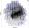 |
Fig. 1. Distribution of VMC tiles across the LMC. The tiles used in this study are those in the outer regions of the galaxy and are indicated by their IDs. The image in the background shows the distribution of all VMC sources. |
Observations were obtained with the VISTA Infrared Camera (VIRCAM) mounted on VISTA1 (Sutherland et al. 2015), which is operated by the European Southern Observatory (ESO). VIRCAM is a near-infrared imaging camera composed of 16 VIRGO HgCdTe detectors. Each detector covers an area of 0.0372 deg2 with an average pixel scale of 0.339″. The individual images from the 16 detectors form a VISTA pawprint that covers 0.6 deg2, not including the gaps between the detectors. A mosaic of six pawprints was used to cover a contiguous area, filling the gaps between individual detectors. This arrangement forms a VMC tile. The individual detector integration time for a Ks-band exposure was 5 s. Taking five jitters and 15 repetitions into account, each point on the sky is observed by two different pixels, so the total exposure amounts to 750 s per tile and epoch. However, in a single pawprint, each pixel is exposed on average for 375 s per tile. There are at least 11 epochs at Ks of this type (deep) and two epochs with half the exposure time (shallow). Exposure times in the Y and J bands as well as additional parameters of the survey are described in detail by Cioni et al. (2011). Images were processed using the VISTA Data Flow System (VDFS) pipeline (v1.5; Emerson et al. 2006) at the Cambridge Astronomy Survey Unit2 and stored in the VISTA Science Archive3 (VSA; Cross et al. 2012). The catalogues provided by the VSA contain aperture photometry that is sufficient to study the relatively moderate stellar density (80 000 stars per deg2 on average) across the outer regions of the LMC. Magnitudes have been calibrated as explained in González-Fernández et al. (2018), which results in an accuracy of better than 0.02 mag in YJKs. The astrometric calibration of the VMC data is based on the Two Micron All-Sky Survey (2MASS; Skrutskie et al. 2006) and carries a systematic uncertainty of 10−20 mas due to World Coordinate System errors4. These systematic uncertainties in the calibration of each detector image obtained using 2MASS stars are mainly caused by atmospheric turbulence and atmospheric differential refraction. Table 1 provides details about the observations. It contains the tile identification, the central coordinates, the orientation, the number of epochs used, their time baseline, the full width at half maximum (FWHM), the airmass, and the sensitivity5 derived from sources with photometric uncertainties < 0.1 mag. The average values of all good quality deep Ks epochs (11 for most tiles) were 0.93 ± 0.10 arcsec (FWHM), 1.49 ± 0.09 (airmass), and 19.28 ± 0.16 mag (sensitivity).
VMC Ks-band observations of the LMC tiles.
3. Analysis
3.1. VMC proper motions
The selection of the sample of VMC sources for which to derive the proper motions, the creation of the astrometric reference frame, and the calculation of the proper motions follow the same steps as described in Schmidt et al. (2020). Some of the steps are repeated here for clarity.
3.1.1. Sample selection
The VMC source catalogues for each tile were obtained from the VSA using a freeform SQL6 query. We extracted equatorial coordinates (right ascension, declination) in J2000, source-type classifications (mergedClass), magnitudes (J and Ks), the corresponding uncertainties, and quality extraction flags (ppErrBits) for each source. VMC tiles, pawprints, and sources in the VSA are identified by their identification numbers: tiles have a unique framesetID, individual pawprints a unique multiframeID, and individual sources a unique sourceID. The source-type classification flags were used to distinguish between stars and galaxies, and quality extraction flags were used to remove low-quality detections by limiting the ppErrBits to 16. This selection criterion removes VMC sources with systematic uncertainties that affect the photometric calibration. The VSA vmcdetection table contains data of the individual pawprints that originate from stacked images. Source catalogues based on individual epoch observations were obtained by cross-matching the list of sources with those in the vmcdetection tables, with all matches within 0.5″ retained. The resulting catalogue contains the mean modified Julian day (MJD) of the observation, the detector number (extNum), the pixel coordinates (x, y) on each detector, and the corresponding positional uncertainties. We split the VMC epoch catalogues into 96 parts (for 6 pawprints × 16 detectors) per epoch and tile, respectively. Distinct epochs were then selected based on their multiframeIDs. All sources with the same multiframeID are part of the same pawprint observed across the 16 detectors. Undesired multiframeIDs, such as those associated with observations from overlapping tiles (where sources would be detected in different detectors), observations obtained under poor sky conditions, and detections at wavelengths other than Ks, were removed. Every catalogue was then divided into two parts. One contains only sources classified as galaxies (mergedClass = 1), and the other contains only stars (mergedClass = −1). We rejected all other source-type classifications (e.g. noise, probable stars, and probable galaxies). In a small number of cases, two sources in the vmcdetection tables, with the same multiframeIDs, were matched to one sourceID from the vmcsource catalogue. This duplication was caused by the matching algorithm when two sources were sufficiently close together in the detection catalogue and one of the sources was missing in the vmcsource catalogue. The nearest source was selected in this case.
3.1.2. Deriving the proper motions
To calculate consistent proper motions, each observation of a given source has to be in the same astrometric reference frame. The reference frames for each VMC tile in this study were created by choosing the epoch with the best observing conditions from each set of observations of a given tile. This corresponds to the epoch with the largest number of extracted sources and the smallest FWHM. The reference frames were constructed using background galaxies. The number of background galaxies in the VMC survey is quite large (a few hundred per detector), and in the outer regions of the LMC there are > 200 per detector with > 300 in less crowded regions. This is sufficient to produce proper motions as accurate as those that can be derived from a reference system made of VMC stars within the same area (Niederhofer et al. 2018). The median rms values from matching the epochs using background galaxies was 0.23 pixels, and all matches had a value smaller than 0.28 pixels. These residuals affect the median proper motion of the background galaxies, resulting in a moving reference frame. To correct the co-moving reference frame, we set the σ-clipped relative median proper motion of the galaxies for each detector to zero. We checked for possible systematic effects, such as unevenly distributed samples, an influence of uncertainties in individual coordinates, and the size of the matching samples. None of these seemed to have a significant influence on the results.
After creating the reference frame, every corresponding epoch catalogue was transformed into it using IRAF7 (Tody 1993) tasks xyxymatch, geomap, and geoxytran and then joined with the reference epoch catalogue of the same pointing and detector. The proper motions of individual stars were calculated by using a linear least-squares fit for the x and y coordinates separately and the corresponding MJD with respect to a reference frame defined by background galaxies. Each fit typically contained 11 data points that spanned an average time baseline of 1230 days (see Table 1 for the time baseline for each tile). Calculations were performed on a detector-by-detector basis for each of the 16 detectors and 6 pawprints of each tile. The slopes of these fits are the proper motions of individual stars for the two components in units of pixels per day. The conversion to mas yr−1 was done using the World Coordinate System information from the FITS headers of the detector images at the reference epoch (see Cioni et al. 2016 for details).
When calculating the median proper motions of a selection of stars, we removed outliers using a 3σ clipping technique, where σ was calculated using the median absolute deviation (MAD). The statistical error was calculated as the MAD divided by the square root of the numbers of stars. The σ-clipping was repeated until no additional sources were removed. We checked the proper motions for any trends with detector number, position on the detectors, and J − Ks colours and found nothing significant that influenced our results. Finally, we derived the near-infrared proper motion of 16 210 461 stellar VMC sources in the outer regions of the LMC (Table 2).
Size of stellar samples.
3.2. Gaia EDR3 sample selection
Gaia EDR3 data were acquired through the Gaia at AIP database8, which provides a cross-match with the VMC source catalogue using a tolerance radius of 1″ and taking the Gaia EDR3 proper motions into account. The sky coordinates for sources in the VMC catalogue refer to the epoch J2000, whereas in the Gaia EDR3 catalogue they refer to J2015.5; both datasets make use of the International Coordinate Reference System. We removed stars that could be problematic sources, such as astrometric binaries, (partially) resolved binaries, or multiple stars blended together using the re-normalised unit weight error (RUWE). As described in Schmidt et al. (2020) and recommended by the Gaia Data Processing and Analysis Consortium, we selected sources with RUWE < 1.40. A check of the residuals of VMC versus Gaia proper motions shows that there are no significant correlations as a function of magnitude, colour, or sky position (see Fig. C.1). VMC proper motions may be unreliable for individual sources, but binning a large number of them (at least a few hundred, depending on the level of contamination between stellar populations, e.g. between LMC and MW stars) shows a good agreement with the Gaia values (Schmidt et al. 2020; Niederhofer et al. 2021). Figure C.2 shows that the dispersion (calculated as maximum minus minimum) of the difference between Gaia EDR3 and VMC proper motions decreases with an increasing number of stars. Here, no distinction has been made between MW and LMC stars or different LMC stellar populations. All Voronoi bins of the VMC measurements agree to better than 0.05 mas yr−1 because the smallest bin contains at least 1600 stars.
A subset of the Gaia EDR3 catalogue, comprising stars with G < 18.5 mag, was selected and combined with the newest STARHORSE distance estimates (Anders et al. 2022) using the unique Gaia sourceID, which both catalogues share. These sources form the basis of our training sample and are further discussed in Sect. 3.3.2. The VMC–Gaia sample, including only sources with a measured parallax, contains fewer than half of the stellar sources in the VMC sample, in total 7 265 212 unique stellar sources, whereas the STARHORSE sample contains only 796 875 sources due to the magnitude limitation. The sample sizes of the catalogues used in this study are shown in Table 2.
3.3. Distinguishing Magellanic Cloud from Milky Way stars
Our previous studies based on the VMC data (Niederhofer et al. 2018, 2021; Schmidt et al. 2019) emphasised the importance of an efficient foreground removal. Although Gaia EDR3 delivers excellent parallax measurements, they still have significant uncertainties for objects at the distance of the Magellanic Clouds. The same is true for Gaia and VMC proper motions. Both parallax and proper motion measurements also become more challenging for fainter sources and, therefore, for the vast majority of stars in the Magellanic Clouds. Simple cuts in parallax and proper motion are only sufficient to remove MW stars among the brightest stars, such as upper red giant branch (RGB) and bright main sequence stars, as shown in, for example, Vasiliev (2018). The uncertainties in parallax and proper motions are significant enough that a large number of MW foreground stars are indistinguishable from the majority of the Magellanic Cloud stars based on parallaxes and proper motions alone. The nature of the overlapping functional distributions leads to an uneven distribution of MW foreground stars within the proper motion spread of the Magellanic Cloud stellar population, as shown by Schmidt et al. (2020) for the part of the LMC close to the Magellanic Bridge and by Gaia Collaboration (2018) for other dwarf galaxies (e.g. Sagittarius). This uneven distribution will always nudge every median measurement towards the MW proper motion value. While this effect can be reduced by removing the majority of the foreground stars using other methods (e.g. using colours and magnitudes), it will persist as long as there are MW stars in the sample.
More sophisticated methods are needed to significantly increase the sample size and enable better spatial resolutions to study the LMC kinematics in detail while also efficiently removing the influence of the MW foreground. Using the distance estimates provided by the Bayesian inference in the STARHORSE code, it is possible to obtain a clean sample of Magellanic Cloud stars, as shown in Schmidt et al. (2020). As described therein, this approach is, however, limited to stars with magnitudes G < 18 mag in the previous STARHORSE version (Queiroz et al. 2018) and G < 18.5 mag in the newest version (Anders et al. 2022). Our new approach bypasses the current magnitude limitation of the STARHORSE distances and enables a more detailed view of the outer LMC regions.
3.3.1. Machine learning with SVM
We used a machine learning classification algorithm called support vector machines (SVMs), which are binary large-margin classifiers and a supervised learning algorithm that evolved based on Boser et al. (1992) and Vapnik (2000). They allow classification information to be transferred from a training set onto unseen data points by mapping the training data with a non-linear transformation to a higher dimensional space to find a separating surface between the two classes. We used an approach similar to a galaxy cluster membership classification (Lopes & Ribeiro 2020) to recover a membership probability from VMC and Gaia EDR3 data in order to efficiently remove MW foreground sources. Our method is based on a combination of astrometric and photometric properties (13 dimensions). They are parallax (ω), parallax error (ω/σω), the two components of proper motion (μαcosδ, μδ) from Gaia and VMC, and multiple magnitudes and colours (J, Ks, J − Ks, G, GRP, GBP, and GRP − BP). Compared to the Bayesian inference method used in the STARHORSE code, SVM is computationally fast since the operation time is independent of the number of sources. As discussed in Sect. 3.3.3, the SVM has been found to be good enough for the purpose of this paper. In the future, radial velocity and element abundances for large samples of stars across the LMC will be provided by the 4-metre Multi-Object Survey Telescope (4MOST; de Jong et al. 2019; Cioni et al. 2019), opening up new possibilities for a more precise membership classification using more parameters as well as a variety of classification methods (e.g. random forest regression and neural network).
3.3.2. SVM classification
A large training set with a reliable MW and LMC separation is hard to obtain, and the combination with STARHORSE, with nearly 800 000 sources, appears sufficient. As such, we did not consider much smaller datasets based on spectroscopic observations or special types of objects, which would not be appropriate for the problem at hand. The classification results for the validation sample represent a viable case for the overall classification, although the training sample is not fully representative, as described below.
Depending on the quality of the data and their uncertainties, it can occur that there is no hyperplane able to separate the two classes of objects (MW and LMC stars) in the training sample. In this case, the algorithm would not converge. To prevent this from happening, we decided to revise the d = 20 kpc criterion used in Schmidt et al. (2020) to separate between MW and Magellanic Bridge stars. The newest STARHORSE data provide a significantly better separation between MW and Magellanic Cloud stars compared to the previous version, although there is still an issue with underestimated distances, as shown in Anders et al. (2022), in the form of an overdensity between the MW and the LMC or other satellites. In the previous STARHORSE version, many Magellanic Cloud sources ended up at significantly shorter or longer distances away from the bulk of the sources that belong to the galaxies. Therefore, stars of the LMC and most of the other MW satellites formed elongated cigar-like structures in all-sky density maps. By adding extra priors for the satellites, this issue was significantly reduced, especially in the outer regions of the Magellanic Clouds. Any remaining overdensity appears associated only with the central regions.
We classified stars with STARHORSE distance estimates smaller than 20 kpc as MW foreground stars and stars farther than 20 kpc as LMC stars. These two samples define the base of the training and validation samples of the SVM classifier. Also, contrary to the previous STARHORSE code, the updated version no longer systematically underestimates the distance of blue LMC stars based on their GBP − GRP colours. In the previous version, those sources occupied the 10−40 kpc range, where there was a significant overlap with the MW foreground population. This overlap blurred the separation between the two classes of objects, and including those sources in the training sets reduced the predictive power of the SVM classification. The new STARHORSE version based on Gaia EDR3 provides a significantly better training sample with respect to the LMC blue stars.
The VMC and Gaia EDR3 cross-matched catalogue contains 796 875 sources with STARHORSE distances. Of them, 553 235 can be clearly classified as either MW (160 438) or LMC stars (636 437) (see Table 2). The actual training sample corresponds to a random fraction of 0.7 from both the MW and LMC. A fraction of 0.3 of the stars is used for validation. We used the python SVM package in the sklearn library9. For a better classification and a higher flexibility of the hyperplane, we tested multiple SVM kernels (e.g. isotonic and sigmoid) with a maximum of 100 000 iterations. Both the isotonic and sigmoid kernels enable more flexibility in the determination of the hyperplane that divides the training sets. This hyperplane is used to classify other sources. We found that the isotonic calibration of the classifier delivered the highest prediction power, with a Brier coefficient of 0.076 and a recall rate of 0.985. The Brier score describes the mean squared error of the prediction and ranges from 0 to 1, with 0 being a perfect calibration. The isotonic regression provides high flexibility, but it is prone to overfitting (Menon et al. 2012). Our tests show that the training sample has sufficient data to avoid this since the isotonic regression outperforms the sigmoid regression (Niculescu-Mizil & Caruana 2005).
The reliability curves of the standard classifier, isotonic, and sigmoid regressions are shown in Fig. 2. The isotonic calibration offers a nearly perfect calibration, closely followed by the sigmoid calibration, while the standard classifier is significantly biased towards the LMC. This is visible as a peak in the mean predicted value at 0.8 in the histogram (Fig. 3). This indicates an increase in falsely classified sources, which illustrates two important facts. First, that the majority of the falsely classified sources are classified as MW stars could be a direct effect of the bias introduced by STARHORSE underestimating the distances of LMC stars, as mentioned before, which is carried over by residuals in the training sample. However, we noticed a significant improvement with respect to the previous STARHORSE version. The classifier became stricter as it classified more LMC stars as foreground stars than in the previous version. This could be due to the uncertainties in the Gaia EDR3 measurements – many of the faint stars have too large uncertainties to be recognised as LMC stars. Second, it proves that there is no simple solution possible in all the provided data columns. The simple SVM kernel does not find a clear separation between both classes as it classifies the majority of the foreground stars as LMC stars, and therefore stricter selections will have a greater impact on the LMC sample size than on the fraction of MW foreground stars.
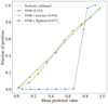 |
Fig. 2. Reliability curves of the predicted values for the three different kernels used in the classification. The reliability curves compare the mean predicted value of a random subsample to the fraction of actual positives in the sample. The numbers between parentheses refer to the Brier score (see Sect. 3.3). |
After training the classifier using variations in the hyperplane through random samples of the training set to increase the separation between the two classes (LMC and MW), the classifier was then used on the extended VMC–Gaia EDR3 catalogue, including faint stars that do not have STARHORSE distances. The SVM classification, using the isotonic calibration, results in 2 629 456 LMC members (Table 2).
A critical factor in machine learning is the choice of the training sample. In Schmidt et al. (2020), we showed that STARHORSE distance estimates could be used to remove a significant fraction of MW foreground stars. Figure 4 shows a comparison between the colour−magnitude diagram (CMD) of the VMC sources with a Gaia EDR3 counterpart and STARHORSE distances for LMC stars (d > 20 kpc), as used in Schmidt et al. (2020), and the majority of MW stars (d < 10 kpc, blue). A selection based on STARHORSE distances is limited to stars with G < 18.5 mag. The LMC stars in the STARHORSE sample are in fact only bright main sequence and giant stars, which excludes a large number of faint Magellanic Cloud stars, such as the red clump stars. At faint magnitudes, there is also a larger number of MW foreground stars.
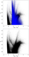 |
Fig. 4. Optical CMDs of sources in the LMC outer regions. Top panel: sources with VMC and Gaia EDR3 photometry as well as STARHORSE distances (black) and the MW stars from our training sample that have STARHORSE distance estimates d < 10 kpc (blue). Bottom panel: likely Magellanic stars with STARHORSE distance estimates d > 20 kpc (based on Schmidt et al. 2020). |
Figure 5 illustrates a near-infrared CMD of the initial VMC-Gaia EDR3 sample compared to the training sample, with the distribution of parallax and parallax error indicated for the latter. This figure shows that the training sample is partly incomplete. A notable fraction of main sequence stars and carbon stars at the tip of the RGB are missing from the training sample. However, while carbon stars are ultimately classified as LMC stars, a significant number of main sequence stars are wrongly classified as MW foreground stars along with a relatively small number of RGB stars (see Fig. 6 for stars classified as MW sources). These RGB stars are incorrectly classified due to the small parallax values in connection with large parallax uncertainties. The majority of properly classified bright MW stars have large parallaxes and small associated uncertainties. On the contrary, the relatively small number of incorrectly classified main sequence stars corresponds to both small parallaxes (< 0.15 mas) and small parallax errors (< 0.25 mas).
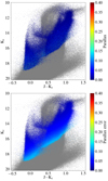 |
Fig. 5. Near-infrared CMD of sources in the training sample, colour-coded by parallax (top) and parallax error (bottom) and superimposed on the VMC and Gaia EDR3 cross-match catalogue (grey). |
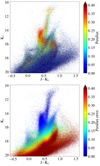 |
Fig. 6. Near-infrared CMD of stars classified as MW foreground sources, colour-coded by parallax (top) and parallax error (bottom). |
3.3.3. SVM tests
A comparison of the previously mentioned classifier calibrations is shown in Table 3. All three classifier calibrations provide a good predictive power; however, both the isotonic and sigmoid calibrations are significantly closer to the best possible score of 0. Although the precision score of the isotonic calibration is slightly lower compared to the sigmoid calibration, the greater flexibility of the isotonic calibration provides a better recall score. We tested several variations of the information provided to the classification algorithm, and multiple tests suggest that classifications without parallax measurements are mostly unreliable. Table 4 compares the percentage of MW stars found in the different regions of the near-infrared CMD by the SVM algorithm with and without the use of parallaxes. The latter shows that significantly fewer stars are classified as MW stars in regions H and F, which are regions clearly dominated by MW stars from star formation history (SFH) studies (e.g. Cioni et al. 2014; El Youssoufi et al. 2019). In CMD regions populated mostly by faint stellar populations (A–E), the SVM classifies in general more stars as MW stars because at these magnitudes the parallax is not reliable, the proper motions are more uncertain, and the efficiency of the other parameters is also reduced due to the limitation of the training sample (cf. Fig. B.2). There are also faint MW stars in regions I and K that are similarly difficult to isolate (see also Niederhofer et al. 2021). The resulting percentage of LMC stars in these regions is perhaps more reliable than complete. However, the use of the parallax parameter decreases the number of MW stars in region A, which also contains bright stars. This is in line with the excellent agreement between the SFH and SVM classifications of stars occupying region G.
SVM classifier calibration.
Percentage of MW stars in different CMD regions.
We found that the photometric VMC data (J, Ks, and J − Ks) add more predictive power to the SVM classifier than the Gaia photometric data (GRP, GBP, and GRP − BP). This is expected because the difference between the colours of MW and LMC stars is greater in the near-infrared than in the optical bands. Mazzi et al. (2021) show that the MW foreground defines a prominent feature at J − Ks = 0.8 mag and a less marked one at J − Ks = 0.4 mag, with most of the LMC stars at J − Ks < 0.7 mag. In the Gaia CMD, the majority of the MW stars have colours that overlap with those of red giants in the LMC (e.g. Vasiliev 2018). On the contrary, the VMC proper motions add no value to the predictive power compared to Gaia EDR3 proper motions. This is also expected because of the large uncertainties associated with the VMC proper motions of individual sources, which create less peaked distributions (Fig. B.2).
When used on the entire STARHORSE sample (not limited to the LMC outer regions), the SVM classifier completely recovers all sources with STARHORSE distances > 20 kpc, which includes the cleanest large sample of stars in the Magellanic Bridge (Schmidt et al. 2020). Trained on the newest STARHORSE data, it also fully recovers the main sequence stars (J − Ks ∼ −0.2 mag), contrary to the classifier trained on the previous STARHORSE data. Compared to the selection criteria presented in the Gaia EDR3 (Gaia Collaboration 2021a), the SVM classification results in a slightly larger number of young stars (∼103), the same number of asymptotic giant branch stars, and a significantly larger number of blue loop stars (∼104) associated with the LMC, whereas it classifies more RGB and red clump stars (∼105) as foreground.
4. Results
To study the kinematics of the outer regions of the LMC, we used a sample of 2 629 456 LMC stars, obtained after removing MW stars as described above. Figure 8 shows the distribution of these stars in the near-infrared CMD, and regions occupied by specific stellar populations are indicated as in El Youssoufi et al. (2019). We used the two-dimensional Voronoi technique (Cappellari & Copin 2003), as in Schmidt et al. (2020), to bin the data in sky coordinates. We used 257 bins, where each bin contains from a hundred to several thousand LMC stars, depending on the selected stellar population as described in Sect. 4.1. We derived the median Gaia EDR3 and VMC proper motions and the corresponding uncertainties of each bin. These values are listed in Tables 5–8, which are available in their entirety only electronically. For each bin we provide its angular distance from the centre of the LMC (Paturel et al. 2003), the number of stars, the proper motion components, and the rotational velocity derived from both the Gaia EDR3 and VMC data. Although we can measure a significantly larger number of proper motions from the VMC survey alone, this advantage is lost due to the requirement of an existing parallax measurement for the SVM algorithm, which we used to remove the MW stars.
Gaia EDR3 proper motion of LMC stars.
Gaia EDR3 proper motion of old stars.
Gaia EDR3 proper motion of young stars.
VMC proper motion of LMC stars.
We used the LMC population of GalMod, the Gaia EDR3 mock catalogue from Rybizki et al. (2020), as a tool to derive the expected proper motion measurements across the outer LMC for a non-rotating spherical galaxy with no internal kinematics. The mock catalogue is constructed as a simple three-dimensional (3D) Gaussian distribution. All the particles are assigned a random 3D velocity centred around the bulk motion of the LMC, which corresponds to 1.95 mas yr−1 in right ascension, 0.43 mas yr−1 in declination, and vR = 283 km s−1 for the radial velocity corrected for the solar reflex motion with respect to the Galactic centre. The mock catalogue proper motions are then derived from the position on the sky, the distance, and 3D velocity. The mock catalogue contains, among other things, a Magellanic Cloud stellar population, which can be queried by its identification number (popid = 10). The sky position of the centre-of-mass of the LMC model is described in Paturel et al. (2003) and corresponds to 80 84 in right ascension and −69
 78 in declination. The overlap between the mock catalogue and the VMC tiles is shown in Fig. 7; the LMC footprint from the VMC survey is entirely covered. As mentioned by Rybizki et al. (2020), the proper motions in the model data should not be compared to the Gaia measurements, since the model does not account for the internal kinematics and components of the galaxy (e.g. disc, rotation, spiral arms, and bar). However, the model data can be used to infer a rotation field, which proves useful in our study. Furthermore, it allows us to correct for the changes in proper motion due to the 3D bulk motion of the LMC (Robin et al. 2012) caused by different viewing angles. We took the shape and size of our Voronoi bins into account and transferred them into the model. The different viewing angles are the only cause of any difference between the median proper motion of these model bins and the central proper motion. We then subtracted the median predicted proper motion of the model bins from the measured median proper motions to remove the LMC bulk motion. This enables the internal kinematics of the LMC to be studied (e.g. rotation) and also corrects the measurements for the differences in viewing angles and the solar reflex motion. Without applying such a correction, the proper motions, especially to the east and west of the LMC, appear significantly higher than overall around the galaxy.
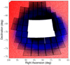 |
Fig. 7. VMC tiles (black) covering the outer regions of the LMC superimposed on the distribution of Gaia EDR3 mock data. MW foreground stars in the mock catalogue are shown in red and LMC stars in blue. |
Furthermore, the proper motion values in the mock catalogue are already corrected for the reflex motion of the Sun10. The space velocity of the Sun adopted for this correction corresponds to the galactocentric velocity (vx = 11.1 km s−1, vy = 239.08 km s−1, vz = 7.25 km s−1), which is different from the latest value derived using Gaia EDR3 data with respect to compact (quasar-like) extragalactic sources (Lindegren et al. 2021). The solar reflex motion influences proper motion measurements depending on the distance of the sources and their position on the sky. While the effect diminishes with distance, it is notable at the distance of the LMC (Fig. A.1). Compared to the Gaia EDR3 values, there is an average offset in the proper motion of 0.01 mas yr−1 in declination and of 0.02 mas yr−1 in right ascension (Fig. A.2). These offsets are at least ten times smaller than the average measurement uncertainties.
4.1. Selection of stellar populations
We used the CMD regions from El Youssoufi et al. (2019) to select different stellar populations (see Fig. 8). Each region is dominated by a class of objects with an associated median age (see Table 1 in El Youssoufi et al. 2019). Compared to El Youssoufi et al. (2019), we find significantly fewer MW foreground stars, especially in region F. Except for stars at the edge of the RGB, this region contains mainly MW foreground sources wrongly classified as LMC sources by the machine learning algorithm. Sources in region F are excluded from the subsequent analysis. Using the remaining CMD regions, we divided the catalogue into two age groups: a young population (< 1 Gyr old) containing stars in the CMD regions A, B, G, H, and I and an older population (> 2 Gyr old) that contains stars in the CMD regions D, E, J, K, and M. This age division is based on average ages of the CMD bins as described in El Youssoufi et al. (2019). We did not use stars in region C because they have ages encompassing both groups. There are 808 515 and 2 738 707 stars in the young and old age group, respectively.
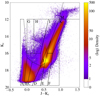 |
Fig. 8. Near-infrared CMD of LMC stars with boxes overlaid to distinguish different populations according to El Youssoufi et al. (2019). |
4.2. Proper motion maps
Figures 9 and 10 show the residual proper motion maps of LMC stars from the Gaia EDR3 and VMC samples, respectively, after subtracting the LMC bulk motion. Both maps show rotation of the LMC, as expected. The rotation is clearly visible in the northern and western regions of the outer LMC, where the north-western and western spiral arms are located. Regions in the east and parts of the south-west also show a visible rotation. Only the south-eastern region, where the south-eastern arm is located, does not show a clear rotation compared to the rest of the galaxy. The residual proper motions are significantly smaller. However, the proper motions of most bins in this region follow the expected direction of the LMC rotation.
 |
Fig. 9. Distribution of stellar proper motions across the LMC from the Gaia EDR3 sample. Each vector represents the median proper motion of at least a few hundred stars. The central vector indicates the bulk motion at the centre of the GalMod model, which was used to create the residual map. The central regions that are characterised by a high stellar density and influenced by crowding issues are not analysed in this study. |
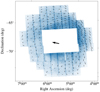 |
Fig. 10. As Fig. 9 but for VMC proper motions. Each vector represents the median proper motion of at least 1600 stars. |
Figure 11 shows residual proper motion maps of our selected stellar populations: < 1 Gyr and > 2 Gyr old (see Sect. 4.1). The old population, which consists of about two-thirds of all LMC stars, shows a smooth rotation, especially in the north. The young population shows a similar behaviour, but for a less coherent motion in the region of the northern arm, where the young population is likely influenced by the morphological structures of the LMC. To better compare the proper motion of old and young stars, we show their differential map (Fig. 12). The differential motion shows a few distinct aspects. Residuals on the northern and north-eastern sides point predominantly towards the north, which could be due to the influence of the MW after the pericentre passage (van der Marel et al. 2002) as this is the direction towards the MW centre. Residuals on the southern and south-eastern sides do not show any preferential motion, which suggests that young and old stars share the same motion. However, residuals in the inner region south, west, and north of the bar show an anti-clockwise rotation, which indicates that young stars move faster than old stars.
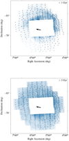 |
Fig. 11. Gaia EDR3 proper motion maps of the LMC for samples of stars < 1 Gyr old (top) and > 2 Gyr old (bottom) (see text for details). Each vector represents the median proper motion of at least 100 stars for the young population and of at least 2000 stars for the old population. The central vector indicates the bulk motion of the LMC as shown in Fig. 9. |
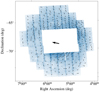 |
Fig. 12. Gaia EDR3 differential proper motion map of the LMC, with the proper motion of the young population (Fig. 11, top) subtracted from that of the old population (Fig. 11, bottom). The proper motion vectors are up-scaled by a factor of ten compared to Fig. 11. |
4.3. Rotation
We used the python package galpy to derive the rotational velocity component with respect to the LMC centre in km s−1 (vϕ) and the median distance to the centre of each Voronoi bin. For the centre we adopted the values 80 84 in right ascension and −69
 78 in declination, which is the value used to produce the Gaia EDR3 mock catalogue (Rybizki et al. 2020). The rotational velocities calculated from all stars within each bin are shown in Fig. 13. The majority of the data points show velocities higher than the Gaia EDR3 rotation curve (e.g. Gaia Collaboration 2021a), but a non-negligible fraction shows below-average rotation speeds. Nearly all bins corresponding to high speeds are located in the north-eastern to western regions of the LMC. The difference between the higher speeds in this study and the Gaia EDR3 measurements are explained by the different binning techniques. The larger sample size in this study eliminates the need for radial binning and therefore enables a more differentiated map of the outer LMC. The velocities for young and old stars show no significant differences from the combined sample. The younger population, however, shows a larger spread due to the larger uncertainties. Similar to their combined sample, the majority of both the young and old stars show a slightly higher rotation speed compared to the Gaia EDR3 results. Contrary to radial binning, which is often used to measure rotation curves, our binning enables a more differentiated map of the outer LMC.
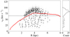 |
Fig. 13. Rotational velocity of the LMC derived from Gaia EDR3 proper motions with respect to the centre of the Gaia EDR3 mock catalogue (black). Each point corresponds to the median velocity within bins in the sky that contain at least a few hundred stars (see text for detail). The red line indicates the Gaia EDR3 measurements (Gaia Collaboration 2021a). The dashed line at 65 km s−1 was chosen based on the histogram to the right of the main diagram. |
Figure 14 shows the median proper motions derived for all stars within the Voronoi bins colour-coded by their rotational speed with the spatial regions defined in Parada et al. (2021) superimposed. These authors illustrated the 3D orientation of the LMC by introducing nine (F1−9) spatial regions. They used carbon stars as standard candles to infer distances from their median J magnitudes. For the LMC they found the region F1 (ΔM̄J = 0.11 mag) to be the farthest away and F9 (ΔM̄J = −0.12 mag) to be the closest, while F7 (ΔM̄J = 0.00 mag), F2/F4 (ΔM̄J = 0.01 mag), F3/F6 (ΔM̄J = −0.04 mag), and F5 (ΔM̄J = −0.02 mag) are at a distance similar to the average distance. Only region F8 (ΔM̄J = 0.07 mag) deviated from expectations, but this was explained by the high extinction surrounding the 30 Doradus star forming region.
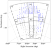 |
Fig. 14. Gaia EDR3 proper motion map of the LMC stars in bins (each containing at least a few thousand stars from different stellar populations), colour-coded by rotational velocity. Black proper motion vectors indicate a rotation speed of less than 65 km s−1 (dashed line in Fig. 13). Regions F1−9 are from Parada et al. (2021). |
The resulting pattern suggests that a part of the LMC (south-east) is rotating slower than expected, which is apparently not correlated with the orientation of the galaxy. We recall that our proper motion maps are not corrected for the inclination of the LMC disc, which may introduce a velocity pattern.
One possible explanation would involve a population of stars connected to the debris of the SMC in the south-eastern regions of the LMC (F4, F7, and F8), which resulted from the last interaction event between the two galaxies (roughly 250 Myr ago). The origin of the material is unclear. It can be stripped SMC material, LMC material influenced by the SMC, or more likely a combination of the two. An N-body simulation finds this event responsible for pulling the Bridge out of the SMC disc (Diaz & Bekki 2012). This debris population apparently connects the young (F1) and old (F4) Bridge and possibly bends around the LMC in the north-east (F9). The connection between the (young) Magellanic Bridge and the Southern Substructure (old Bridge) coincides with the locations found by Belokurov et al. (2017) and El Youssoufi et al. (2021).
4.4. Influence of the SMC impact
To interpret the velocity pattern of the LMC stars, we compared the map shown in Fig. 9 with an N-body model of the LMC–SMC system from Diaz & Bekki (2012). For this model, the authors adopted an orbital history in which the LMC and the SMC became an interacting pair about 2 Gyr ago. As a result of their first encounter, the SMC is disrupted, several tidal structures are created, and a large fraction of the material stripped away from the SMC is engulfed by the LMC. Figure 15 shows the proper motion of the LMC stars superimposed on the density distribution of the N-body simulation. The motion of the N-body particles (indicated with red arrows) is mainly towards the west, and the predicted distribution of the SMC debris spans the area from the south-west to the north-east of the galaxy. The slower rotational speed of LMC stars in the south-east compared to those in other areas could result from the influence of the SMC.
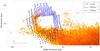 |
Fig. 15. Gaia EDR3 proper motions of the full sample of LMC stars, without distinguishing between young and old stellar populations, superimposed on the model density distribution of stripped SMC stars (Diaz & Bekki 2012). The proper motion vectors are colour-coded by the rotational velocity, with stars rotating slower than 65 km s−1 indicated in black and those rotating faster indicated in blue. Each arrow corresponds to the ensemble velocity of at least a few thousand stars. The red arrows indicate the median proper motion of the N-body particles. |
A kinematically distinct component due to the SMC was found by Olsen et al. (2011, 2015) from the analysis of about 6000 spectra of giant stars. The authors derived both radial velocities and metallicities to conclude that about 5% of their stellar sample originated in the SMC. These stars, after being subsequently captured by the LMC together with gas, might have triggered the intense star formation in the 30 Doradus region. The rotational pattern of these suspected SMC stars opposes the LMC rotation by more than 50 km s−1. This velocity translates to a proper motion of about 0.2 mas yr−1 at the distance of the LMC, which is within the uncertainties of both our VMC and Gaia EDR3 proper motion measurements. However, assuming we have detected the influence of the SMC stars in the south-east of the LMC, this suggests that either the velocity difference is larger than 50 km s−1 or that the fraction of stars sharing this velocity is significantly larger. Assuming that these stars move as predicted by the N-body simulation (Diaz & Bekki 2012), we would expect a fraction of about 6%, which is in good agreement with the results found by Olsen et al. (2015). It is interesting that the percentages of kinematically distinct stars agree despite the differences between the two stellar samples. Our sample includes a broad range of stellar populations: from main sequence to red clump stars, the bright part of the RGB, and other evolved giants (Fig. 8). The sample used by Olsen et al. (2015) is limited to Ks < 12 mag and contains predominantly massive red supergiants and asymptotic giant branch stars, including carbon stars.
Indu & Subramaniam (2015) modelled the neutral atomic hydrogen kinematics of the LMC and found that about 12% of the data points deviate from that of a disc. These points trace various features, possibly caused by tidal and/or hydrodynamical effects. In the south-east of the galaxy, the gas is rotating slower than in the main disc, which is similar to what we find in our study. Indu & Subramaniam (2015) suggest that an infall of gas from the Magellanic Bridge, to the south-west, would explain the counter-rotating component identified by Olsen et al. (2011) and the slow rotation in the south-east, the latter resulting from the drag of the rotating component.
The tidal force of the MW during the LMC infall could also influence the rotational speed by stretching the LMC in a direction perpendicular to the bar. However, this effect does not seem to be very strong, especially in the southern regions of the galaxy (Fig. 12). A better understanding of the particular region of the LMC influenced by the recent SMC pericentre (∼150 Myr ago) and the disc crossings (400 Myr ago and older) (see e.g. Cullinane et al. 2022 for the location of these events) as well as a separation of the LMC and SMC stars will be crucial to explain the kinematic properties of the galaxy.
5. Conclusions
In this study we have continued our investigation of the outer regions of the Magellanic system. We combined the VMC data with data from the Gaia EDR3 to study the outer regions of the LMC. We introduced a new method to distinguish between Magellanic and MW stars, based on a machine learning algorithm trained on STARHORSE distance estimates, to improve our analysis by significantly increasing the usable sample size. Our membership classification provides the largest catalogue of LMC stars with a distance between 1.5 and 6.2 kpc from the centre of the galaxy. With this technique, we are able to study the kinematics of faint stellar populations below the red clump of the LMC. We have shown residual proper motion maps (after subtracting the bulk motion) of two populations (< 1 and > 2 Gyr old). Both populations showed a distinct motion in the south-eastern outer region of the galaxy compared to the other directions. For the first time, we found hints of stripped SMC debris in the proper motion of stars located in the south-east of the outer LMC. This supports findings by Olsen et al. (2011) based on radial velocities of giant stars that suggested a counter-rotating population in that region. The current uncertainties of the proper motions are, however, insufficient to separate those stars from possible LMC stars whose motion might have been influenced by interaction with the SMC.
In the future, projects such as the 4MOST will provide a large sample of radial velocities for different stellar populations across the Magellanic Clouds (Cioni et al. 2019), which are currently missing, to determine the fraction of SMC stars accreted by the LMC. It may also be possible to determine if individual stars belong to the LMC or the SMC via chemical tagging. So far, it is unclear if these stars, which rotate more slowly than the average rotational speed in the outer region of the LMC, are leftovers from the SMC interaction or if the rotational direction of LMC stars has changed as a result of the interaction between the two galaxies.
Structured Query Language (SQL); http://horus.roe.ac.uk:8080/vdfs/VSQL_form.jsp
Image Reduction and Analysis Facility; https://iraf-community.github.io/
Acknowledgments
This project has received funding from the European Research Council (ERC) under the European Union’s Horizon 2020 research and innovation programme (grant agreement no. 682115). We thank the Cambridge Astronomy Survey Unit (CASU) and the Wide Field Astronomy Unit (WFAU) in Edinburgh for providing the necessary data products under the support of the Science and Technology Facility Council (STFC) in the UK. This research was also supported in part by the Australian Research Council Centre of Excellence for All Sky Astrophysics in 3 Dimensions (ASTRO 3D), through project number CE170100013. This project has made extensive use of the Tool for OPerations on Catalogues And Tables (TOPCAT) software package (Taylor 2005) as well as the following open-source Python packages: Astropy (Astropy Collaboration 2018), matplotlib (Hunter 2007), NumPy (Oliphant 2015), Numba, and Pyraf.
References
- Anders, F., Khalatyan, A., Queiroz, A. B. A., et al. 2022, A&A, 658, A91 [NASA ADS] [CrossRef] [EDP Sciences] [Google Scholar]
- Astropy Collaboration (Price-Whelan, A. M., et al.) 2018, AJ, 156, 123 [Google Scholar]
- Belokurov, V., Erkal, D., Deason, A. J., et al. 2017, MNRAS, 466, 4711 [Google Scholar]
- Besla, G., Kallivayalil, N., Hernquist, L., et al. 2007, ApJ, 668, 949 [Google Scholar]
- Besla, G., Hernquist, L., & Loeb, A. 2013, MNRAS, 428, 2342 [NASA ADS] [CrossRef] [Google Scholar]
- Besla, G., Martínez-Delgado, D., van der Marel, R. P., et al. 2016, ApJ, 825, 20 [Google Scholar]
- Boser, B. E., Guyon, I. M., & Vapnik, V. N. 1992, Proceedings of the Fifth Annual Workshop on Computational Learning Theory, COLT ’92 (New York, NY, USA: Association for Computing Machinery), 144 [CrossRef] [Google Scholar]
- Cappellari, M., & Copin, Y. 2003, MNRAS, 342, 345 [Google Scholar]
- Cioni, M. R. L., Clementini, G., Girardi, L., et al. 2011, A&A, 527, A116 [CrossRef] [EDP Sciences] [Google Scholar]
- Cioni, M. R. L., Girardi, L., Moretti, M. I., et al. 2014, A&A, 562, A32 [NASA ADS] [CrossRef] [EDP Sciences] [Google Scholar]
- Cioni, M.-R. L., Bekki, K., Girardi, L., et al. 2016, A&A, 586, A77 [NASA ADS] [CrossRef] [EDP Sciences] [Google Scholar]
- Cioni, M. R. L., Storm, J., Bell, C. P. M., et al. 2019, The Messenger, 175, 54 [NASA ADS] [Google Scholar]
- Cross, N. J. G., Collins, R. S., Mann, R. G., et al. 2012, A&A, 548, A119 [NASA ADS] [CrossRef] [EDP Sciences] [Google Scholar]
- Cullinane, L. R., Mackey, A. D., Da Costa, G. S., et al. 2022, MNRAS, 510, 445 [Google Scholar]
- de Jong, R. S., Agertz, O., Berbel, A. A., et al. 2019, The Messenger, 175, 3 [NASA ADS] [Google Scholar]
- Di Teodoro, E. M., McClure-Griffiths, N. M., Jameson, K. E., et al. 2019, MNRAS, 483, 392 [Google Scholar]
- Diaz, J. D., & Bekki, K. 2012, ApJ, 750, 36 [Google Scholar]
- El Youssoufi, D., Cioni, M.-R. L., Bell, C. P. M., et al. 2019, MNRAS, 490, 1076 [NASA ADS] [CrossRef] [Google Scholar]
- El Youssoufi, D., Cioni, M.-R. L., Bell, C. P. M., et al. 2021, MNRAS, 505, 2020 [NASA ADS] [CrossRef] [Google Scholar]
- Emerson, J., Irwin, M., & Hambly, N. 2006, Proc. SPIE, 6270, 62700S [NASA ADS] [CrossRef] [Google Scholar]
- Erkal, D., Belokurov, V., Laporte, C. F. P., et al. 2019, MNRAS, 487, 2685 [Google Scholar]
- Gaia Collaboration (Helmi, A., et al.) 2018, A&A, 616, A12 [NASA ADS] [CrossRef] [EDP Sciences] [Google Scholar]
- Gaia Collaboration (Luri, X., et al.) 2021a, A&A, 649, A7 [EDP Sciences] [Google Scholar]
- Gaia Collaboration (Brown, A. G. A., et al.) 2021b, A&A, 650, C3 [EDP Sciences] [Google Scholar]
- Gardiner, L. T., & Noguchi, M. 1996, J. Korean Astron. Soc., 29, S93 [Google Scholar]
- González-Fernández, C., Hodgkin, S. T., Irwin, M. J., et al. 2018, MNRAS, 474, 5459 [Google Scholar]
- Hammer, F., Yang, Y. B., Flores, H., Puech, M., & Fouquet, S. 2015, ApJ, 813, 110 [NASA ADS] [CrossRef] [Google Scholar]
- Hashimoto, Y., Funato, Y., & Makino, J. 2003, ApJ, 582, 196 [CrossRef] [Google Scholar]
- Hunter, J. D. 2007, Comput. Sci. Eng., 9, 90 [NASA ADS] [CrossRef] [Google Scholar]
- Indu, G., & Subramaniam, A. 2015, A&A, 573, A136 [NASA ADS] [CrossRef] [EDP Sciences] [Google Scholar]
- Kruijssen, J. M. D., Pfeffer, J. L., Chevance, M., et al. 2020, MNRAS, 498, 2472 [NASA ADS] [CrossRef] [Google Scholar]
- Lindegren, L., Klioner, S. A., Hernández, J., et al. 2021, A&A, 649, A2 [EDP Sciences] [Google Scholar]
- Lopes, P. A. A., & Ribeiro, A. L. B. 2020, MNRAS, 493, 3429 [NASA ADS] [CrossRef] [Google Scholar]
- Martin, N. F., Ibata, R. A., Bellazzini, M., et al. 2004, MNRAS, 348, 12 [Google Scholar]
- Mazzi, A., Girardi, L., Zaggia, S., et al. 2021, MNRAS, 508, 245 [NASA ADS] [CrossRef] [Google Scholar]
- McClure-Griffiths, N. M., Dénes, H., Dickey, J. M., et al. 2018, Nat. Astron., 2, 901 [CrossRef] [Google Scholar]
- Menon, A., Jiang, X., Vembu, S., Elkan, C., & Ohno-Machado, L. 2012, Proceedings of the 29th International Conference on Machine Learning, ICML 2012, 1 [Google Scholar]
- Mucciarelli, A., Bellazzini, M., Ibata, R., et al. 2017, A&A, 605, A46 [NASA ADS] [CrossRef] [EDP Sciences] [Google Scholar]
- Niculescu-Mizil, A., & Caruana, R. 2005, Proceedings of the 22nd International Conference on Machine Learning, ICML ’05 (New York, NY, USA: Association for Computing Machinery), 625 [Google Scholar]
- Niederhofer, F., Cioni, M.-R. L., Rubele, S., et al. 2018, A&A, 612, A115 [NASA ADS] [CrossRef] [EDP Sciences] [Google Scholar]
- Niederhofer, F., Cioni, M.-R. L., Rubele, S., et al. 2021, MNRAS, 502, 2859 [Google Scholar]
- Niederhofer, F., Cioni, M. R. L., Schmidt, T., et al. 2022, MNRAS, 512, 5423 [NASA ADS] [CrossRef] [Google Scholar]
- Olsen, K. A. G., Zaritsky, D., Blum, R. D., Boyer, M. L., & Gordon, K. D. 2011, ApJ, 737, 29 [CrossRef] [Google Scholar]
- Olsen, K. A. G., Blum, R. D., Smart, B., et al. 2015, in Fifty Years of Wide Field Studies in the Southern Hemisphere: Resolved Stellar Populations of the Galactic Bulge and Magellanic Clouds, eds. S. Points, & A. Kunder, ASP Conf. Ser., 491, 257 [NASA ADS] [Google Scholar]
- Parada, J., Heyl, J., Richer, H., Ripoche, P., & Rousseau-Nepton, L. 2021, MNRAS, 501, 933 [Google Scholar]
- Patel, E., Besla, G., & Sohn, S. T. 2017, MNRAS, 464, 3825 [NASA ADS] [CrossRef] [Google Scholar]
- Paturel, G., Petit, C., Prugniel, P., et al. 2003, A&A, 412, 45 [NASA ADS] [CrossRef] [EDP Sciences] [Google Scholar]
- Pearson, S., Privon, G. C., Besla, G., et al. 2018, MNRAS, 480, 3069 [NASA ADS] [CrossRef] [Google Scholar]
- Oliphant, T. E. 2015, Guide to NumPy (Scotts Valley: CreateSpace) [Google Scholar]
- Queiroz, A. B. A., Anders, F., Santiago, B. X., et al. 2018, MNRAS, 476, 2556 [Google Scholar]
- Robin, A. C., Luri, X., Reylé, C., et al. 2012, A&A, 543, A100 [NASA ADS] [CrossRef] [EDP Sciences] [Google Scholar]
- Rybizki, J., Demleitner, M., Bailer-Jones, C., et al. 2020, PASP, 132, 074501 [Google Scholar]
- Schmidt, T., Cioni, M. R., Niederhofer, F., Diaz, J., & Matijevic, G. 2019, in Dwarf Galaxies: From the Deep Universe to the Present, eds. K. B. W. McQuinn, & S. Stierwalt, IAU Symp., 344, 130 [Google Scholar]
- Schmidt, T., Cioni, M.-R. L., Niederhofer, F., et al. 2020, A&A, 641, A134 [NASA ADS] [CrossRef] [EDP Sciences] [Google Scholar]
- Skrutskie, M. F., Cutri, R. M., Stiening, R., et al. 2006, AJ, 131, 1163 [NASA ADS] [CrossRef] [Google Scholar]
- Stanimirović, S., Staveley-Smith, L., & Jones, P. A. 2004, ApJ, 604, 176 [Google Scholar]
- Sutherland, W., Emerson, J., Dalton, G., et al. 2015, A&A, 575, A25 [NASA ADS] [CrossRef] [EDP Sciences] [Google Scholar]
- Taylor, M. B. 2005, in Astronomical Data Analysis Software and Systems XIV, eds. P. Shopbell, M. Britton, & R. Ebert, ASP Conf. Ser., 347, 29 [Google Scholar]
- Tody, D. 1993, in Astronomical Data Analysis Software and Systems II, eds. R. J. Hanisch, R. J. V. Brissenden, & J. Barnes, ASP Conf. Ser., 52, 173 [Google Scholar]
- van der Marel, R. P., & Kallivayalil, N. 2014, ApJ, 781, 121 [Google Scholar]
- van der Marel, R. P., Alves, D. R., Hardy, E., & Suntzeff, N. B. 2002, AJ, 124, 2639 [NASA ADS] [CrossRef] [Google Scholar]
- Vapnik, V. 2000, The Nature of Statistical Learning Theory, 8, 1 [Google Scholar]
- Vasiliev, E. 2018, MNRAS, 481, L100 [Google Scholar]
- Zivick, P., Kallivayalil, N., Besla, G., et al. 2019, ApJ, 874, 78 [Google Scholar]
- Zivick, P., Kallivayalil, N., & van der Marel, R. P. 2021, ApJ, 910, 36 [Google Scholar]
Appendix A: Solar reflex motion
The outer regions of the LMC cover large parts of the sky. On this scale, there is an effect on the proper motion measurements caused by the reflex motion of the sun. The effect is illustrated in Fig. A.1. The difference on the opposite side (west and east) is of the same order as the statistical uncertainties. We found no significant difference when comparing the reflex motion used in the mock catalogue and the updated values (Fig. A.2).
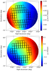 |
Fig. A.1. Effect of the solar reflex motion across the LMC on the proper motion components, μαcos(δ) (top) and μδ (bottom), as used in the Gaia EDR3 mock catalogue. |
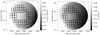 |
Fig. A.2. Difference between the effect of the solar reflex motion in the Gaia EDR3 mock catalogue and as measured with the data across the LMC on the proper motion components: μαcos(δ) (left) and μδ (right). |
Appendix B: Source classification
Most LMC sources that were wrongly classified as MW foreground sources (main sequence and RGB stars) can be found in regions with a high stellar density, for example close to the bar and the northern spiral arms (see Fig. B.1). Figure B.2 compares the distribution of stars from the full catalogue, the training sample, and the stars classified by the machine learning algorithm as belonging to the LMC and MW, respectively, for each of the 13 parameters used by the algorithm.
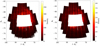 |
Fig. B.1. Spatial distribution of sources classified as LMC members (left) and MW foreground stars (right). Higher densities in the overlapping regions of tiles are due to duplication in the VMC data as they represent independent measurements. |
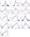 |
Fig. B.2. Histograms of the distribution of the number of stars with respect to the 13 parameters used by the machine learning algorithm. The training sample is shown in green, whereas the full catalogue is shown in black. Magenta and blue lines refer instead to the distributions of LMC and MW stars, respectively, as classified by the algorithm. |
Appendix C: VMC and Gaia proper motions
The proper motion differences between Gaia EDR3 and VMC as a function of parallax, colour, magnitude, and position show that there is no obvious correlation (Fig. C.1). The consistency between VMC and Gaia proper motions was also discussed in Niederhofer et al. (2021).
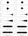 |
Fig. C.1. Proper motion differences between Gaia EDR3 and VMC as a function of: parallax (ω), J − Ks colour, G magnitude, Ks magnitude, right ascension, and declination (from top to bottom) for both components of motion (from left to right). |
The dispersion of the difference between VMC and Gaia proper motions in relation to the number of stars in each bin is shown in Fig. C.2. The average dispersion of 50 random samples of stars across the LMC (including both LMC and MW stars) drops below the average measurement uncertainty of individual stars around 100 and approaches zero for roughly 500 stars. Each Voronoi bin in the final VMC catalogues contains significantly more stars (at least 1600), which indicates a good agreement between the two datasets.
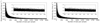 |
Fig. C.2. Dispersion of the differences between Gaia EDR3 and VMC proper motion in right ascension (left) and declination (right) for 50 random stellar samples with different sizes, as indicated along the horizontal axis. The zoomed-in panels are centred at the number of stars corresponding to the smallest bin of Fig. 10. |
All Tables
All Figures
|
Fig. 1. Distribution of VMC tiles across the LMC. The tiles used in this study are those in the outer regions of the galaxy and are indicated by their IDs. The image in the background shows the distribution of all VMC sources. |
| In the text | |
|
Fig. 2. Reliability curves of the predicted values for the three different kernels used in the classification. The reliability curves compare the mean predicted value of a random subsample to the fraction of actual positives in the sample. The numbers between parentheses refer to the Brier score (see Sect. 3.3). |
| In the text | |
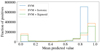 |
Fig. 3. Histogram of the predicted values shown in Fig. 2. |
| In the text | |
|
Fig. 4. Optical CMDs of sources in the LMC outer regions. Top panel: sources with VMC and Gaia EDR3 photometry as well as STARHORSE distances (black) and the MW stars from our training sample that have STARHORSE distance estimates d < 10 kpc (blue). Bottom panel: likely Magellanic stars with STARHORSE distance estimates d > 20 kpc (based on Schmidt et al. 2020). |
| In the text | |
|
Fig. 5. Near-infrared CMD of sources in the training sample, colour-coded by parallax (top) and parallax error (bottom) and superimposed on the VMC and Gaia EDR3 cross-match catalogue (grey). |
| In the text | |
|
Fig. 6. Near-infrared CMD of stars classified as MW foreground sources, colour-coded by parallax (top) and parallax error (bottom). |
| In the text | |
|
Fig. 7. VMC tiles (black) covering the outer regions of the LMC superimposed on the distribution of Gaia EDR3 mock data. MW foreground stars in the mock catalogue are shown in red and LMC stars in blue. |
| In the text | |
|
Fig. 8. Near-infrared CMD of LMC stars with boxes overlaid to distinguish different populations according to El Youssoufi et al. (2019). |
| In the text | |
|
Fig. 9. Distribution of stellar proper motions across the LMC from the Gaia EDR3 sample. Each vector represents the median proper motion of at least a few hundred stars. The central vector indicates the bulk motion at the centre of the GalMod model, which was used to create the residual map. The central regions that are characterised by a high stellar density and influenced by crowding issues are not analysed in this study. |
| In the text | |
|
Fig. 10. As Fig. 9 but for VMC proper motions. Each vector represents the median proper motion of at least 1600 stars. |
| In the text | |
|
Fig. 11. Gaia EDR3 proper motion maps of the LMC for samples of stars < 1 Gyr old (top) and > 2 Gyr old (bottom) (see text for details). Each vector represents the median proper motion of at least 100 stars for the young population and of at least 2000 stars for the old population. The central vector indicates the bulk motion of the LMC as shown in Fig. 9. |
| In the text | |
|
Fig. 12. Gaia EDR3 differential proper motion map of the LMC, with the proper motion of the young population (Fig. 11, top) subtracted from that of the old population (Fig. 11, bottom). The proper motion vectors are up-scaled by a factor of ten compared to Fig. 11. |
| In the text | |
|
Fig. 13. Rotational velocity of the LMC derived from Gaia EDR3 proper motions with respect to the centre of the Gaia EDR3 mock catalogue (black). Each point corresponds to the median velocity within bins in the sky that contain at least a few hundred stars (see text for detail). The red line indicates the Gaia EDR3 measurements (Gaia Collaboration 2021a). The dashed line at 65 km s−1 was chosen based on the histogram to the right of the main diagram. |
| In the text | |
|
Fig. 14. Gaia EDR3 proper motion map of the LMC stars in bins (each containing at least a few thousand stars from different stellar populations), colour-coded by rotational velocity. Black proper motion vectors indicate a rotation speed of less than 65 km s−1 (dashed line in Fig. 13). Regions F1−9 are from Parada et al. (2021). |
| In the text | |
|
Fig. 15. Gaia EDR3 proper motions of the full sample of LMC stars, without distinguishing between young and old stellar populations, superimposed on the model density distribution of stripped SMC stars (Diaz & Bekki 2012). The proper motion vectors are colour-coded by the rotational velocity, with stars rotating slower than 65 km s−1 indicated in black and those rotating faster indicated in blue. Each arrow corresponds to the ensemble velocity of at least a few thousand stars. The red arrows indicate the median proper motion of the N-body particles. |
| In the text | |
|
Fig. A.1. Effect of the solar reflex motion across the LMC on the proper motion components, μαcos(δ) (top) and μδ (bottom), as used in the Gaia EDR3 mock catalogue. |
| In the text | |
|
Fig. A.2. Difference between the effect of the solar reflex motion in the Gaia EDR3 mock catalogue and as measured with the data across the LMC on the proper motion components: μαcos(δ) (left) and μδ (right). |
| In the text | |
|
Fig. B.1. Spatial distribution of sources classified as LMC members (left) and MW foreground stars (right). Higher densities in the overlapping regions of tiles are due to duplication in the VMC data as they represent independent measurements. |
| In the text | |
|
Fig. B.2. Histograms of the distribution of the number of stars with respect to the 13 parameters used by the machine learning algorithm. The training sample is shown in green, whereas the full catalogue is shown in black. Magenta and blue lines refer instead to the distributions of LMC and MW stars, respectively, as classified by the algorithm. |
| In the text | |
|
Fig. C.1. Proper motion differences between Gaia EDR3 and VMC as a function of: parallax (ω), J − Ks colour, G magnitude, Ks magnitude, right ascension, and declination (from top to bottom) for both components of motion (from left to right). |
| In the text | |
|
Fig. C.2. Dispersion of the differences between Gaia EDR3 and VMC proper motion in right ascension (left) and declination (right) for 50 random stellar samples with different sizes, as indicated along the horizontal axis. The zoomed-in panels are centred at the number of stars corresponding to the smallest bin of Fig. 10. |
| In the text | |
Current usage metrics show cumulative count of Article Views (full-text article views including HTML views, PDF and ePub downloads, according to the available data) and Abstracts Views on Vision4Press platform.
Data correspond to usage on the plateform after 2015. The current usage metrics is available 48-96 hours after online publication and is updated daily on week days.
Initial download of the metrics may take a while.