© ESO 2019

1. Introduction

The morphology of the stellar disk of our Galaxy has been explored in recent years (e.g., Juric et al. 2008; Reylé et al. 2009; Mateu et al. 2011; Polido et al. 2013; López-Corredoira & Molgó 2014; Xu et al. 2015; Bovy et al. 2016), which has led to a global picture of the density laws with their exponential radial and vertical dependences, together with their corresponding scale length and scale height, asymmetries, flare, warp, subdivision of a thin+thick component, and other features. The chemical abundances of the thin and thick disks were also widely explored (e.g., Rong et al. 2001; Ak et al. 2007; Casagrande et al. 2011; Haywood et al. 2013; Hayden et al. 2015) showing the different gradients of metallicities and alpha-enhancement. However, the kinematics of the disk is not so well known, and we have only very recently begun to gather relevant information away from the solar neighbourhood; see for example, Bond et al. (2010), Siebert et al. (2011), Williams et al. (2013), Carrillo et al. (2018), Wang et al. (2018) and the set of three papers by one of the current authors dedicated to the azimuthal, vertical, and radial Galactocentric components, respectively: López-Corredoira (2014), López-Corredoira et al. (2014), López-Corredoira & González-Fernández (2016).

The Gaia mission of the European Space Agency (Gaia Collaboration 2016) is leading us into a new era of the study of the kinematics of our Galaxy. Gaia offers the position of each star in six-dimensional (6D) phase space: three dimensions of spatial information plus three dimensions of velocity. Gaia data provide accurate distance determination for nearby sources, but the errors increase with distance from us. For this reason, the Gaia Collaboration (2018b; hereafter G18) and Kawata et al. (2018) carried out a kinematical analysis of the second data release (DR2) of the Gaia sample including radial velocities only for Galactocentric radii R ≲ 13 kpc, which is a reachable range for stars with relative error in distance lower than 20%. However, there is a large number of Gaia-DR2 stars beyond R = 13 kpc that may allow for larger distances to be explored, where several interesting features, such as the warp, flare, and others, are known to develop. Poggio et al. (2018) extended the analyzed region up to R ≲ 15 kpc in combination with 2MASS photometry, but only paid attention to the vertical motions. We can extend the Gaia maps much more than that limit: indeed our aim here is to provide maps of velocities up to R ≈ 20 kpc, using a technique to recover information on the 3D motions through a deconvolution of the Gaussian errors in the parallaxes, applicable even for large errors. In a forthcoming work, we will consider the dynamical models that may explain the kinematical properties discussed here.

The paper is organized as follows: in Sect. 2, we describe the Gaia data that we use in this paper; in Sect. 3, we explain the method for the conversion of heliocentric to Galactocentric coordinates and for the deconvolution used to obtain information even with large errors; the results of the application of the method to the real data is described in Sect. 4; a discussion to sum up the paper, with our conclusions, is given in the final section.

2. Gaia-DR2 data

We use here the data of the second Gaia data release (Gaia DR2; Gaia Collaboration 2018a) for the stars with available radial heliocentric velocities: 7 224 631 sources, from which we take only those with parallax error less than 100% (7 103 123 sources), observed with a Radial Velocity Spectrometer (RVS; Cropper et al. 2018) that collects medium-resolution spectra (spectral resolution $\frac{\lambda }{\mathrm{\Delta }\lambda }\approx 11700$) over the wavelength range 845–872 nm centered on the calcium triplet region. This radial velocity data set contains the median radial velocities, averaged over the 22 month time span of the observations. The sources are nominally brighter than twelfth magnitude in the G_RVS photometric band, most having magnitudes brighter than 13 in the G filter.

Radial velocities are only reported for stars with effective temperatures in the range 3550–6900 K. The uncertainties of the radial velocities are: 0.3 km s⁻¹ at G_RVS <  8, 0.6 km s⁻¹ at G_RVS = 10, and 1.8 km s⁻¹ at G_RVS = 11.75; plus systematic radial velocity errors of < 0.1 km s⁻¹ at G_RVS <  9 and 0.5 km s⁻¹ at G_RVS = 11.75. For details on radial velocity data processing and the properties and validation of the resulting radial velocity catalogue, see Sartoretti et al. (2018) and Katz et al. (2018). The set of standard stars that was used to define the zero-point of the RVS radial velocities is described in Soubiran et al. (2018).

Here we do not consider any possible zero-point bias in the parallaxes of Gaia-DR2 as found by some authors (Lindegren et al. 2018; Arenou et al. 2018; Stassun & Torres 2018; Zinn et al. 2018), except in Sect. 4.4 where we repeat some of the key calculations with a non-zero value of the zero-point in order to show that its effect on our main results is negligible.

3. Obtaining the Galactocentric velocity

The information provided by the Gaia-DR2 catalog for each star contains the parallax π, the Galactic coordinates (ℓ, b), the radial velocity ν_r and the two proper motions in equatorial coordinates μ_α cosδ and μ_δ (which can be transformed into Galactic coordinates as μ_ℓ cosb and μ_b). These six variables allow for each star to be placed in the 6D phase space: 3D spatial+3D velocity.

The Galactocentric position in cylindrical coordinates has the following three components: the Galactocentric distance R, the Galactocentric azimuth ϕ¹, and the vertical distance Z. Analogously, the Galactocentric velocity in cylindrical coordinates has the following three components: the radial velocity V_R, the azimuthal velocity V_ϕ, and the vertical velocity V_Z. The convention for the sign for the Galactocentric radial velocity is positive when directed outwards. The conversion formulas are the following (López-Corredoira & González-Fernández 2016):

$$\begin{array}{cc}& r=\frac{1\mathrm{AU}}{\pi }\hfill \\ \hfill & X(r,\ell ,b)=R_{\odot }-rcos\ell cosb,\hfill \\ \hfill & Y(r,\ell ,b)=rsin\ell cosb,\hfill \\ \hfill & Z(r,b)=Z_{\odot }+rsinb,\hfill \\ \hfill & R(r,\ell ,b)=\sqrt{X^2+Y^2},\hfill \\ \hfill & \varphi (r,\ell ,b)={tan}^{-1}\left(\frac{Y}{X}\right)(\mathrm{between}\frac{\pi }{2}\mathrm{and}\frac{3\pi }{2}\mathrm{for}X<0),\hfill \end{array}$$(1)

and

$$\begin{array}{cc}& \mathit{V}(r,\ell ,b,{\nu }_r,{\mu }_{\ell },{\mu }_b)=\hfill \\ \hfill & \left(\begin{array}{c}{V}_R\\ V_{\varphi }\\ V_z\end{array}\right)=\left(\begin{array}{ccc}-cos\varphi & sin\varphi & 0\\ sin\varphi & cos\varphi & 0\\ 0& 0& 1\end{array}\right)\left(\begin{array}{c}{U}_{\ast }+U_{\odot }\\ V_{\ast }+V_{\mathrm{g},\odot }\\ W_{\ast }+W_{\odot }\end{array}\right),\hfill \\ \hfill & \left(\begin{array}{c}{U}_{\ast }\\ V_{\ast }\\ W_{\ast }\end{array}\right)=\left(\begin{array}{ccc}cos\ell cosb& -sin\ell & -cos\ell sinb\\ sin\ell cosb& cos\ell & -sin\ell sinb\\ sinb& 0& cosb\end{array}\right)\left(\begin{array}{c}{\nu }_r\\ {\nu }_{\ell }\\ {\nu }_b\end{array}\right),\hfill \\ \hfill & {\nu }_{\ell }=r{\mu }_{\ell }cosb,\hfill \\ \hfill & {\nu }_b=r{\mu }_b.\hfill \end{array}$$(2)

Here we adopt the same Galactic parameters used by the previous kinematic Gaia-DR2 analysis (G18): R_⊙ = 8.34 kpc (Reid et al. 2014), Z_⊙ = 0.027 kpc (Chen et al. 2001); (U_⊙, V_⊙, W_⊙)=(11.1, 12.24, 7.25) km s⁻¹ (Schönrich et al. 2010); V_g, ⊙ = V_c, ⊙ + V_⊙, with the rotation speed V_c, ⊙ = 240 km s⁻¹ (Reid et al. 2014).

3.1. Deconvolution of parallax errors

The main problem to solve is the deconvolution of the Gaussian errors with large root mean square (rms) values. The large dispersion of parallaxes (and hence the large dispersion of distances) affect the value of mean distance at large heliocentric distances, which is indeed overestimated in a direct measurement with respect to the real one. This occurs because the parallax errors grow with distance and because of a selection effect: most of the stars in a bin centered at r are indeed at a much lower distance for the observational asymmetry, meaning that there are much more stars at distances < r than at distances > r. The symmetric parallax uncertainties (σ_π) produce asymmetric distance uncertainties, with a probability distribution function stretched toward larger distances: the largest the relative uncertainty on the parallax, the largest the asymmetry.

Let us explain this point in more detail. The number of stars per unit parallax that we see in a given line of sight is $\overline{N}(\pi )$. However, this is not the true number of stars per unit parallax, N(π), but its convolution with a Gaussian function that takes into account the measurement error, that is,

$$\begin{array}{c}\hfill \overline{N}(\pi )={\displaystyle {\int }_0^{\infty }\mathrm{d}{\pi }^{\prime }N({\pi }^{\prime })G_{{\pi }^{\prime }}(\pi -{\pi }^{\prime }),}\end{array}$$(3)

and

$$\begin{array}{c}\hfill G_{\pi }(x)=\frac{1}{\sqrt{2\pi }{\sigma }_{\pi }}{\mathrm{e}}^{-\frac{x^2}{2{\sigma }_{\pi }^2}}.\end{array}$$(4)

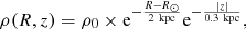
We take as σ_π the average error on π given by the Gaia-DR2 survey computed for the stars of each bin. We note that N(π) contains the dependence of the stellar density along the line of sight multiplied by the selection factors:

$$\begin{array}{c}\hfill N(\pi )=\omega \frac{\rho (1/\pi )}{{\pi }^4}{\displaystyle {\int }_{-\infty }^{m_{G,\lim }-5{log}_{10}(1/\pi )-10-A_G(1/\pi )}\mathrm{d}{M}_G{\varphi }_G(M_G),}\end{array}$$(5)

where ω is the covered angular surface of the line of sight (in stereoradians), ρ(r) is the stellar density along the line of sight, ϕ_G(M_G) is the luminosity function in the G filter as a function of the absolute magnitude M_G, m_G, lim is the limiting maximum apparent magnitude of the survey (in our case m_G, lim is between 12 and 13) and A_G(r) is the cumulative extinction out to a distance of r.

Equation (3) is a Fredholm integral equation of the first kind with kernel equal to G_π(π − π′). The inversion of this equation can be carried out and thus we can obtain a solution N(π) from the observed data $\overline{N}(\pi )$. For that, we use here an iterative Bayesian method called Lucy’s method that is detailed in Appendix A. The integrals are discretized with bins of width Δπ = 0.01 mas; the results do not change with the variation of Δπ, but the resolution and the range of the explored range depend on it. There are also other methods of Gaussian deconvolution in the literature appropriate for different kinds of physical problems (e.g., Masry & Rice 1992; Fang et al. 1994; Ulmer 2010, 2013), but an iterative method is more appropriate here because it is more robust against noise.

Once we have obtained the deconvolved distribution of sources along the line of sight, we estimate the mean heliocentric distance of all the stars included in a bin of parallax π and the corresponding variance:

$$\begin{array}{cc}& \overline{r}(\pi )=\frac{1}{\overline{N}(\pi )}{\displaystyle {\int }_0^{\infty }\mathrm{d}{\pi }^{\prime }\frac{N({\pi }^{\prime })}{{\pi }^{\prime }}{G}_{{\pi }^{\prime }}(\pi -{\pi }^{\prime }),}\hfill \end{array}$$(6)

$$\begin{array}{c}\\ \hfill & {\sigma }_{\overline{r}}^2(\pi )=\left[\frac{1}{\overline{N}(\pi )}{\displaystyle {\int }_0^{\infty }\mathrm{d}{\pi }^{\prime }\frac{N({\pi }^{\prime })}{\pi {{}^{\prime }}^2}{G}_{{\pi }^{\prime }}(\pi -{\pi }^{\prime })}\right]-\overline{r}{(\pi )}^2.\hfill \end{array}$$(7)

For obtaining the variance in the positive and in the negative parts separately, the expressions would be similar to Eqs. (3) and (8) but with integral limits (0,$1/\overline{r}(\pi )$] and ($1/\overline{r}(\pi )$,∞), respectively.

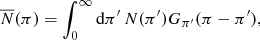
In Fig. 1 we show how the Galactocentric distance R changes when taking into account this deconvolution, for a particular line of sight in the direction of the anticenter. In the anticenter direction the correction is negligible for R ≲ 13 kpc, but becomes very important beyond that radius. For the stars with measured R ≈ 35 kpc (r ≈ 27 kpc, π ≈ Δπ = 0.037 mas; that is, the case with 100% error in heliocentric distance), we get that the mean average value of R is indeed ≈18 kpc. This gives us an idea of the limits of Gaia DR2, either with or without radial velocities: we cannot go beyond ≈20 kpc, and most of the stars with measured larger distance are indeed stars with much lower distance but with a large positive error.

Fig. 1. Galactocentric distance R, obtained after the deconvolution of the heliocentric distances through Eq. (6), vs. R, obtained from the heliocentric distances as 1/π (see Eq. (1)). For comparison, the dashed line (y = x) shows how the Galactocentric distance R should behave without the deconvolution correction. This result is obtained for the Gaia-DR2 data including νr measurements with the constraints: |ℓ−180 ° | <  20°, |b|< 10°, $\frac{\pi }{\mathrm{\Delta }\pi }>1$.

It is worth stressing that the Lucy’s method is model independent, that is, we can recover information on the stellar distribution without introducing any prior. This is necessary if one does not know a priori that information. Other Bayesian methods used to deconvolve Gaussian errors of Gaia parallaxes (e.g., Astraatmadja & Bailer-Jones 2016; Bailer-Jones et al. 2018) make use of a prior on the density of the Milky Way to improve the determination of the distances, meaning that they are model dependent.

Unfortunately, we cannot apply the same method of inversion to obtain the different component of V: Lucy’s method only works with positive magnitudes, and other analytical inversion methods are less robust as there is a degeneracy of solutions in a combination of positive and negative values that limits the inversion possibilities. Nonetheless, we can calculate the distribution of the velocity V as a function of R with the deconvolution correction according to the above prescription: that is, $\mathit{V}(\overline{r},\ell ,b,{\nu }_r,{\mu }_{\ell },{\mu }_b)$ as a function of $R(\overline{r},\ell ,b$), using the transformations of Eqs. (1) and (2); in each bin with mean distance $\overline{r}$, we recalculate the velocities as a function of the recalculated Galactocentric distance. An example is given in Fig. 2, for the R, ϕ, and Z components, respectively, in the direction towards the anticenter. We also show in Fig. 3 the number of stars per unit parallax before and after deconvolution; as can be observed, the application of the method significantly decreases the number of stars with low π. We note that the plotted velocities are the median values within a range of distances R whose rms value is indicated by the horizontal error bars.

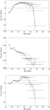Fig. 2. Median of Galactocentric radial (top panel) azimuthal (middle panel) and vertical (bottom panel) velocity as a function of $R(\overline{r})$ (R with a deconvolution correction according to Sect. 3.1). This is the result for Gaia-DR2 data including νr measurements with the constraints: |ℓ−180 ° | <  20°, |b|< 10°, $\frac{\pi }{\mathrm{\Delta }\pi }>1$. Vertical bars indicate the errors on the median velocity (without including the uncertainty in distance). Horizontal bars indicate the rms value of the mean deconvolved R (thus the indicated value is an average over that range of dispersion).

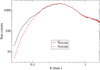Fig. 3. Log–log plot of the observed counts of stars $\overline{N}\mathrm{\Delta }\pi$ (with a bin width Δπ = 0.01 mas.) as a function of the parallax, together with the calculated star counts NΔπ after the deconvolution was applied, for the Gaia-DR2 with measured radial velocity and with the constraints: |ℓ−180 ° | <  20°, |b|< 10°, $\frac{\pi }{\mathrm{\Delta }\pi }>1$.

3.2. Monte Carlo simulations to test the inversion technique

In order to test the method explained in Sect. 6, we present here the results of several Monte Carlo simulations. In our numerical experiments we assume a simple Galactic model with stellar density

$$\begin{array}{c}\hfill \rho (R,z)={\rho }_0\times {\mathrm{e}}^{-\frac{R-R_{\odot }}{2\mathrm{kpc}}}{\mathrm{e}}^{-\frac{|z|}{0.3\mathrm{kpc}}},\end{array}$$(8)

and with a luminosity function ϕ(M) for the disk taken from Bahcall & Soneira (1980). These are rough measurements of the density and of the luminosity function, but here they are not used with any purpose of analysis of the true Milky Way distribution, but only to construct simple tests of the Lucy’s method. We take m_max = 13, R_⊙ = 8.3 kpc as limiting magnitude, and we assume two different radial velocity distributions as a function of the heliocentric distance r: (i) V_R(km s⁻¹)=13 − R(kpc); (ii) $V_R(\mathrm{km}{\mathrm{s}}^{-1})=10sin(1.5\times [\sqrt{R/(1\mathrm{kpc})}-\sqrt{R_{\odot }/(1\mathrm{kpc})]})$. We also take the azimuthal velocity V_ϕ(km s⁻¹)=240 for R <  10 kpc, $V_{\varphi }(\mathrm{km}{\mathrm{s}}^{-1})=240\sqrt{(10\mathrm{kpc})/R}$ for R ≥ 10 kpc, and we take a vertical velocity V_z(km s⁻¹)=20 sin[R/(10 kpc)]. We apply a deconvolution of Gaussian errors assuming σ_π = 0.04 milliarcseconds. We assume an error of heliocentric velocity measurements of 2 km s⁻¹ (i.e., of the order of magnitude of the value between 1.4 and 3.7 km s⁻¹ for the faintest sources according to G18) and an error on proper motions of 0.07 mas yr⁻¹, typical of Gaia-DR2 (G18).

In Figs. 4–7 we show the results of our Monte Carlo simulations for the different components of the velocity and several different directions in the plane. We compare the “initial” assumed V with the one that we measure directly “before deconvolution”, which departs very significantly from the initial V, and the “final” result once we apply the deconvolution. The horizontal error bars indicate the rms value of the mean deconvolved R (thus the indicated value is an average over that range of dispersion). We see that, within the error bars, the recovered value of V agrees with the initial one, except for V_ϕ along ℓ = 60° because the uncertainties in the radial Galactocentric distance are so large that a large uncertainty in the separation of radial and azimuthal components along this line of sight is produced. We see below that these lines of sight are not useful, precisely because of that. We also note that, while the direct measurement of R gives values up to 30 kpc in the anticenter, the corrected deconvolved values of R ≲ 18 kpc. As expected, the large errors in parallax for distant sources is placing some stars beyond what can be observed, but the correction adequately reduces the range.

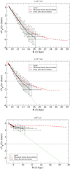Fig. 4. Monte Carlo simulation of VR: with an initial VR( km s−1)=13 − R( kpc), the direct measurement “before deconvolution”, and the “final” result once the deconvolution has been applied. Horizontal error bars indicate the rms value of the mean deconvolved R (thus the indicated value is an average over that range of dispersion). The three panels are for the directions in the planes ℓ = 180°, ℓ = 120°, and ℓ = 60°, respectively.

Fig. 5. As in Fig. 4 but with initial velocity $V_R(\mathrm{km}{\mathrm{s}}^{-1})=10sin(1.5\times [\sqrt{R/(1\mathrm{kpc})}-\sqrt{R_{\odot }/(1\mathrm{kpc})]})$.

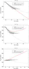Fig. 6. Monte Carlo simulation of Vϕ. Horizontal error bars indicate the rms value of the mean deconvolved R (thus the indicated value is an average over that range of dispersion). The three panels are for the directions in the plane ℓ = 180°, ℓ = 120° and ℓ = 60°, respectively.

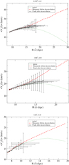Fig. 7. Monte Carlo simulation of Vz. Horizontal error bars indicate the rms value of the mean deconvolved R (thus the indicated value is an average over that range of dispersion). The three panels are for the directions in the plane ℓ = 180°, ℓ = 120° and ℓ = 60°, respectively.

The bias of differences within the noise between “final” and “initial” velocities depends on the function and the direction, meaning that there is not always positive or negative systematic error. Due to the asymmetry in the distribution (larger number of sources at lower heliocentric distances than farther away), the obtained values of velocities in the bins for large R tend to give values at slightly smaller R. One could try to correct this effect by assuming a priori the density distribution of stars, but we avoid the introduction of any prior in our method. We note that the determination of N(π) will not change if we change the velocity field; however, the Lucy’s method introduces a bias that can affect the calculation of $\mathit{V}(\overline{r})$: the effect of such a bias depends on the velocity field itself, as we observe here.

4. Extended region kinematics

We can now apply the above method to obtain the median V. In Figs. 8–12 we plot the results in the Galactic plane of all stars with Δπ <  π and the following constraints on coordinates:

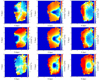Fig. 8. Left panels: three components (radial, azimuthal, and vertical, from top to bottom, respectively) of the Galactocentric velocity Median(V) as a function of $X(\overline{r})$ and $Y(\overline{r})$ (X, Y with deconvolution correction according to Sect. 3.1). Application for Gaia-DR2 data including νr measurement with the constraints: |b|< 10°, $\frac{\pi }{\mathrm{\Delta }\pi }>1$. Inner green contour represents the region with error equal to 10, 10, and 2 km s−1 for VR, Vϕ, and VZ, respectively. Middle panels: error (in log scale) of V derived from the expansion in the formulae of $\mathrm{\Delta }\overline{r}={\sigma }_{\overline{r}}$ as systematic error and the dispersion of values of νr, μℓ, and μb divided by the root square of the number of points per bin as statistical errors. Right panels: rms value of V (corrected for measurement errors). Data of this figure are available at the CDS.

1. |b|< 10°: this gives a wider range in Z for larger distance from the Sun, while in the solar neighbourhood ($\overline{r}\sim 1$ kpc) it is constrained to Z ≲ 0.2 kpc, and at $\overline{r}\sim 10$ kpc it is constrained to Z ≲ 2 kpc. This is enough to sample most disk stars, including the effect of the flare in the outermost disk. Certainly, in the center of the Galaxy (R ≲ 4 kpc) we are overexploring the region of the disk and we are also including the bulge component. The sky within the constraint was divided into 36 lines of sight, each of them with Δℓ=10°, and in each of these cells we have applied the above deconvolution technique.

2. 160 ° < ℓ< 200°: in the anticenter region, which is a region where velocity errors are the lowest, we explore the dependence on vertical distance. The sky was divided into 36 lines of sight, each of them with Δb = 5°, and for those areas we have applied the above deconvolution technique.

3. As in 2. but for 120 ° < ℓ< 160°.

4. As in 2. but for 200 ° < ℓ< 240°.

5. As in 2. but for −20 ° < ℓ< 20°.

In all figures, only the bins with number of stars N ≥ 6 are plotted. For the mean error on V, we assume, from the propagation of the errors, that

$$\begin{array}{c}\hfill \mathrm{\Delta }\overline{r}={\sigma }_{\overline{r}};\end{array}$$(9)

this is a systematic error, so it cannot be reduced by the increase of the number of stars N in each bin. In addition, we include in the propagation of errors,

$$\begin{array}{c}\hfill \mathrm{\Delta }{\nu }_r=\frac{\sigma ({\nu }_r)}{\sqrt{N}};\mathrm{\Delta }{\mu }_{\ell }=\frac{\sigma ({\mu }_{\ell })}{\sqrt{N}}\mathrm{and}\mathrm{\Delta }{\mu }_b=\frac{\sigma ({\mu }_b)}{\sqrt{N}},\end{array}$$(10)

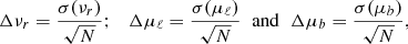
so these are interpreted as statistical errors that can be reduced by increasing the number of stars. Here we neglect the covariance terms in the errors on μ_ℓ, μ_b, and $\overline{r}$: that is, we assume these errors are independent from each other and thus we neglect that these quantities are not derived in isolation and that there may be some correlation between them (Lury et al. 2018, Sect. 2.2). The rms values plotted in the right panels of Fig. 8 were corrected (subtracted quadratically) from the measurement errors in ν_r, μ_ℓ, and μ_b; however, we have not taken into account the variations of V due to the dispersion of r with the deconvolution (i.e., we neglect ∇V) and there may also remain some residuals in high-error regions. In Fig. 8, uncertainties on V_R and V_ϕ are smaller towards the anticenter because the separation of both components is independent of the distance. Moreover, V_R only depends on ν_r, so it is insensitive to the errors on the distance for that reason too. In Figs. 9–12, there are larger uncertainties towards the Galactic pole due to the low number of sources with our binning with constant Δb.

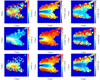Fig. 9. Left panels: three components (radial, azimuthal and vertical, from top to bottom, respectively) of the Galactocentric velocity median (V) as a function of $R=X(\overline{r})$ and $Z(\overline{r})$ (X, Z with deconvolution correction according to Sect. 6). Application for Gaia-DR2 data including νr measurement with the constraints: 160 ° < ℓ< 200°, $\frac{\pi }{\mathrm{\Delta }\pi }>1$. Inner red contour represents the region with error equal to 10 km s−1. Middle panels: error (in log scale) of V derived from the expansion in the formulae of $\mathrm{\Delta }\overline{r}={\sigma }_{\overline{r}}$ as systematic error and the dispersion of values of νr, μℓ, and μb divided by the root square of the number of points per bin as statistical errors. Right panels: rms value of V (corrected for measurement errors). Data of this figure are available at the CDS.

The results for $\overline{r}<4$ kpc are very similar to those of Fig. 10 (for |z|< 0.2 kpc) and Fig. 11 (for |ϕ|< 15°) of G18 with the same Gaia-DR2 data: this corroborates the reliability of our analysis in the common range of distances. However, as we discuss in the following subsections, the most interesting features are observed at larger heliocentric distances, where our analyses provide a novel contribution.

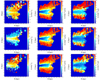Fig. 10. As in Fig. 9 (V(R, Z), its error and rms value) for 120 ° < ℓ< 160°. Data of this figure are available at the CDS.

4.1. Radial velocities

The median radial velocities, their errors, and the rms values are plotted in the three top panels of Figs. 8–12 respectively.

Regions in the top-middle panel of Fig. 8 with yellow-red colors indicate the areas with errors larger than ∼10 km s⁻¹, thus indicating where the median velocities are not accurate. The regions in white-blue tones have errors lower than 10 km s⁻¹, darker blue being indicative of errors lower than 1 km s⁻¹. In the X − Y plane, a prominent feature within low-error regions (ΔV_R ≲ 10 km s⁻¹) is represented by the gradient of velocities along the Y direction with X >  10 kpc: between positive median values of V_R ∼ +20 km s⁻¹ at X >  12 kpc and 2 <  Y(kpc) < 10 (in orange color in top-left panel of Fig. 8) and V_R ∼ −20 km s⁻¹ at X >  16 kpc and −8 <  Y( kpc) < 0 (in medium blue in top-left panel of Fig. 8). Hence, we have a scenario of expansion (stars moving outwards) in the second quadrant and contraction (stars moving inwards) in the third quadrant, and a transition between both areas in a line approximately between (X = 10, Y = −5) and (X = 18, Y = 0) with a radial velocity gradient between these two regions of about 40 km s⁻¹. This is also shown in Fig. 13.

Furthermore, the variation along the center-Sun-anticenter direction shows a change of sign of the radial velocity: positive for X <  8 kpc, negative for 8 <  X( kpc) < 10 and positive for 10 <  X( kpc) < 16 kpc. This is also observed in the top panel of Fig. 2.

This same behavior has already been noted for regions with R ≲ 13 kpc (Siebert et al. 2011; Williams et al. 2013; Wang et al. 2018; Carrillo et al. 2018; G18), and there are even works that reached R ≈ 16 kpc (López-Corredoira & González-Fernández 2016; Tian et al. 2017).

By examining the dependence with Z in the regions where the errors are lower than 5 km s⁻¹ (i.e., the blue regions of the top-middle panels of Fig. 9–11) we may notice that there is more contribution from these positive velocities in the anticenter (Fig. 9) at X >  10 kpc and Z <  0 than at Z >  0, but not in other azimuths. This is also similar to the results in Wang et al. (2018) only for R <  13 kpc. We think that the special feature of the anticenter with respect to this asymmetry is real, but it has nothing to do with systematic effects towards that line of sight as we could not identify any source of systematic error in the data. The fact that this is found at ϕ ≈ 0 and not in other azimuths is therefore a coincidence.

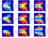Fig. 11. As in Fig. 9 (V(R, Z), its error and rms value) for 200 ° < ℓ< 240°. Data of this figure are available at the CDS.

The values of σ(V_R) plotted in the top-right panel of Figs. 8–12 show no abnormality: σ(V_R) is higher for lower R or larger |Z|. The values and the trends are in agreement with previous estimations: for example, Williams et al. (2013); G18. For ℓ = 0 (Fig. 12: middle-right), σ(V_ϕ) is dominated by large uncertainties towards the Galactic center.

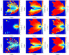Fig. 12. As in Fig. 9 (V(R, Z), its error and rms value) for −20 ° < ℓ<  + 20°. Data of this figure are available at the CDS.

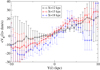Fig. 13. Radial Galactocentric velocity median as a function of $Y(\overline{r})$ for different $X(\overline{r})$ (ΔX = 0.5 kpc) within |b|< 10°.

4.2. Azimuthal velocities

The median azimuthal velocities, their error, and the rms values are plotted in the three middle row panels, from left to right, respectively, of Figs. 8–12.

Regions in the middle panel of Fig. 8 with yellow, orange, and red colors indicate the areas with errors larger than ∼10 km s⁻¹, thus highlighting where the median velocities are inaccurate. The regions in white and light-blue tones have errors lower than 10 km s⁻¹, the darker blue being indicative of errors lower than 1 km s⁻¹. In the X − Y plane, within low-error regions (ΔV_ϕ ≲ 10 km s⁻¹), apart from some small fluctuations there is a clear decrease of the azimuthal velocity for R >  10 kpc: that is, we find²V_ϕ ≲ 220 km s⁻¹ for R >  12 kpc, but V_ϕ(R_⊙)≈240 km s⁻¹. This is also observed in the middle panel of Fig. 2. We note however that higher R also means higher average |Z| (since we have a constant range of Galactic latitude), so part of this decrease is due to a larger ratio of high |Z|-pagination stars.

Figure 9 (left column, middle row) provides a more surprising insight into the distribution of azimuthal velocities towards the anticenter. If we pay attention only to low-error pixels (ΔV_R ≲ 10 km s⁻¹, that is, excluding the regions in orange and red in the central panel of Fig. 9), we see a clear decrease of velocity for larger |Z|, and, moreover, we see an asymmetry by which the velocity is higher for Z <  0 than for Z >  0 in the range 12 <  R( kpc) < 16.

In the top part of Fig. 14, we show ⟨V_ϕ(r)⟩ plots for different Z values with the constraints |ℓ−180 ° | <  20° and |ℓ| <  20°, and observe the same trend. In general for low R <  12 kpc, we see a symmetric distribution with respect to the midplane decreasing with |Z|; for 12 <  R( kpc) < 16, there is a decrease of velocity only for Z >  0 while for negative Z it remains flat and starts to decrease for Z ≲ −3.5 kpc; and for R >  16 kpc it remains almost flat without decrease with Z. However, again this asymmetry is only observed towards the anticenter direction, but not along the lines of sight ℓ = 140°, ℓ = 220 ° , and ℓ = 0 (Figs. 10–12: left column, middle row). We also highlight the radial gradient in Fig. 14, a trend already noted in Fig. 2 (middle) which represents the integral in Z within the limits of |b|< 10 deg. of Fig. 14.

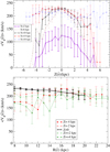Fig. 14. Azimuthal Galactocentric velocity median as a function of $Z(\overline{r})$ for different cuts of constant and $R=X(\overline{r})$ (ΔX = 0.2 kpc) (top panel) or as a function of $R=X(\overline{r})$ for different cuts of $Z(\overline{r})$ (bottom panel). Application for Gaia-DR2 data including νr measurement with the constraints: −20 ° < ℓ< 20° (only top panel) or 160 ° < ℓ< 200°, $\frac{\pi }{\mathrm{\Delta }\pi }>1$.

The monotonous decrease for R ≳ 12 kpc in the plane (Z = 0) has already been found in multiple works for the rotation curve (e.g., Dias & Lépine 2005; Bovy et al. 2012; Kafle et al. 2012; Reid et al. 2014; López-Corredoira 2014; Galazutdinov et al. 2015; G18), although we must bear in mind that an asymmetric drift correction (Bovy et al. 2012; Golubov et al. 2013) remains to be applied and some part of this decrease might be attributed to this correction. The asymmetry north-south has not gained as much attention, although López-Corredoira (2014), for example, already noted its existence for R <  16 kpc, similarly to Wang et al. (2018) and Kawata et al. (2018) for R = 11 − 12 kpc. Furthermore, careful examination of Fig. 13 (left) of G18 reveals some asymmetry at the maximum reached, R ≈ 13 kpc. A decrease of the azimuthal velocity with |Z| was also previously known, although with less-precise data and studying a lower R range than here (e.g., Bond et al. 2010; Bobylev & Bajkova 2010; Williams et al. 2013; López-Corredoira 2014; Wang et al. 2018; G18). The extremely low value given by López-Corredoira (2014) of V_ϕ = 82 ± 5(stat.) ± 58(syst.) km s⁻¹ at R = 16 kpc and Z = 2 kpc dominated by the anticenter stars is not confirmed here to be as low, but we get V_ϕ = 204.8 ± 17.1 km s⁻¹ for that position towards the anticenter; we note however that these values are compatible within 2σ.

Like in the case of radial velocities, the values of σ(V_ϕ) plotted in the middle-right panel of Figs. 8–11 do not reveal any surprises either: σ(V_ϕ) is higher for lower R or larger |Z|. For ℓ = 0 (Fig. 12: middle-right) σ(V_ϕ) is dominated by large uncertainties towards the Galactic center. The values and the trends are in agreement with previous estimations (e.g., Williams et al. 2013; G18), although extending here to larger values of R. We note that thin and thick disks are included here and show differing rotation dispersion between them (Haywood et al. 2013).

4.3. Vertical velocities

The median vertical velocities, their error and the rms values are plotted respectively in the three bottom panels of Figs. 8–12.

Regions in the bottom-middle panel of Fig. 8 with white, yellow, and red colors indicate the areas with errors larger than ∼2.0 km s⁻¹. The regions with blue tones have errors lower than 2.0 km s⁻¹, with darker blue being indicative of errors lower than 1.0 km s⁻¹. In the X − Y plane, a prominent feature within significant detection regions (|V_Z|/ΔV_Z >  3) is the gradient of velocities approximately along the X direction: between a minimum negative median value of V_Z = −3.5 ± 1.1 km s⁻¹ at (X = 9.4, Y = −2.8) and V_Z = +8.8 ± 2.4 km s⁻¹ at (X = 15.6, Y = 1.8). In general, there is a trend of positive V_Z for R ≳ 12 kpc and negative V_Z for R ≲ 12 kpc. As shown in Fig. 15, the gradient is also present with respect to the azimuth. In this figure, we also observe that the radial gradient in V_Z becomes significant when comparing the green diamonds (R = 12 kpc) and the blue triangles (R = 16 kpc). The bottom row of Fig. 9 provides evidence that a larger contribution to positive V_Z, with values even larger than +10 km s⁻¹, comes from the southern hemisphere in the anticenter direction: the north-south asymmetry is clear. For other lines of sight different from the anticenter, we also see asymmetries, but larger in amplitude for ℓ = 220° (Fig. 11: bottom), and with opposite sign for ℓ = 140° (Fig. 10: bottom). Towards the center (Fig. 12: bottom), no asymmetry is observed.

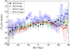Fig. 15. Vertical Galactocentric velocity median as a function of $\varphi (\overline{r})$ for different Galactocentric radii (ΔR = 0.5 kpc) within |b|< 10°.

López-Corredoira et al. (2014) in a sample within the range 5 <  R(kpc) < 16 noticed both the north-south asymmetry and the trend that V_Z increases with R, but found a different absolute value of these velocities and their azimuthal dependence. This is not surprising as the data considered by López-Corredoira et al. (2014) were very noisy and they only got a detection within 2-σ, which we could interpret as a random fluctuation. Liu et al. (2017), Wang et al. (2018), Kawata et al. (2018), and G18 also noted both the north-south asymmetry and the increase of V_Z with R, but measured only up to R = 13 − 14 kpc. Liu et al. (2017) indeed observed that stars with ages < 2 Gyr present a significantly a positive vertical velocity in the anticenter higher than the red clumps with age > 2 Gyr. Also, Widrow et al. (2012), Williams et al. (2013), and Carrillo et al. (2018) observed some of these features but only for regions within 2 kpc of the Sun. Finally, it is worth mentioning that Poggio et al. (2018) observed similar maps using Gaia+2MASS out to R = 15 kpc.

Like in the case of radial velocities, the values of σ(V_Z) plotted in the bottom-right panel of Figs. 8–11 do not reveal any surprises either: σ(V_Z) is higher for lower R or larger |Z|, and in this case also for larger r associated to larger values of average |b|, explaining the red ring in the bottom-right panel of Fig. 8. The values and the trends are in agreement with previous estimations (e.g., Williams et al. 2013, G18), although extending here to larger values of R. For ℓ = 0 (Fig. 12/bottom-right) σ(V_Z) is dominated by large uncertainties towards the Galactic center. We again note that thin and thick disks are included here and display differing vertical dispersion between them (Haywood et al. 2013).

4.4. Effect of a global zero-point bias in the parallaxes

Up to now, we have not considered any possible zero-point bias in the parallaxes of Gaia-DR2. The most accurate measurements indicate that there is a systematic bias of −0.03 mas (Lindegren et al. 2018, Sect. 5.2; Arenou et al. 2018, Sect. 4.4) in the sense that the Gaia-DR2 parallaxes are smaller than the true value, apart from statistical errors.

By repeating our calculations of Fig. 8 with a corrected parallax π_c = π + 0.03 mas, we obtained the results shown in Fig. 16. The results are very similar and deserve the same considerations as those already described above for Fig. 8. The only difference is the very large error bar pixels that show a better trend with this correction, but these pixels were not taken into account in the previous comments so the conclusions remain the same. A similar situation occurs also with the X − Z plots. A higher zero-point bias was also calculated by Stassun & Torres (2018) or by Zinn et al. (2018) but it had the same order of magnitude, so the effect of its correction must be of the same order.

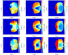Fig. 16. As in Fig. 8, this time introducing a correction to the zero-point bias of parallaxes πc = π + 0.03 mas. Data of this figure are available at the CDS.

5. Discussion and conclusions

An analysis on the dynamical interpretation of these extended kinematic maps will be given in a forthcoming paper (Part II of this paper, in prep.). Nonetheless, without entering here into a discussion about the possible theoretical scenarios, we provide a few notes and considerations from a purely observational point of view.

First, it is clear that our Galaxy is not an axisymmetric system at equilibrium where orbits are purely circular, that is, with V_R = V_Z = 0 and V_ϕ(R, ϕ, Z)=V_ϕ(R); this is especially true for the outer disk. Many other authors have recently reached this same conclusion (e.g., Antoja et al. 2018; G18; Kawata et al. 2018). The presence of a radial and azimuthal velocity gradient of about 40 km s⁻¹, of a vertical velocity gradient of 10 km s⁻¹, and of the north-south asymmetry, with in general higher speeds in the southern Galactic hemisphere, are remarkable characteristics that clearly indicate that the disk of the Milky Way is not an axisymmetric system at equilibrium, but that it is characterized by streaming motions in all three velocity components.

In addition we confirm that the azimuthal velocity is not flat for R >  R_⊙. Even taking account constant Z strips (see Fig. 14) rather than constant b cuts, we see some decrease of the azimuthal velocity: at R = 18 kpc it is ≈10% lower than at R = R_⊙. Other authors (e.g., Galazutdinov et al. 2015) have also noted the fall-off of this velocity, which is more significant for R >  15 kpc. However, here we have computed only the average velocity in some bins of stars as a function of their position with respect to the center of the Galaxy, which is not strictly equal to the rotation speed and needs to be corrected by the asymmetric drift, whose expected correction value is ≲20 km s⁻¹ in the Galactic plane (Bovy et al. 2012; Golubov et al. 2013) and larger for Z ≠ 0 given the higher values of velocity dispersions in off-plane regions (G18). It is possible that the total dependence of V_ϕ on Z, or at least part of it, may be explained by this effect. This is something that we will explore in Part II of this paper, together with other calculations related to dynamics and the Jeans equations (Kafle et al. 2012).

Vertical motions are small, constrained to be within an absolute value lower than 10 km s⁻¹, and present some patterns of oscillation and gradients and are different in general for the northern and southern Galactic hemispheres. Other north-south asymmetries in V_R or V_ϕ only show up in the anticenter direction.

Future analyses of Gaia data with the use of the deconvolution of parallax errors by means of Lucy’s method of inversion, which we discuss in this work, will allow the explored region to R to be increased far beyond 20 kpc, both because future data releases of Gaia will provide a much deeper magnitude limit in the subsample including radial velocities, and because the parallax errors will also be much lower. The range of distances covered by studies using only stars with distance errors < 20% (such as the one that was done by G18) will be increased with the future data releases; however by considering the deconvolution method we have discussed here, one can obtain information at heliocentric distances that are two to three times larger than results without applying error deconvolution techniques. Furthermore, the present method can also be used to obtain the density ρ(r) along the line of sight once we know the luminosity function, even for larger error in parallaxes, by means of Eqs. (3) and (5), which is another application that will allow us to extend our knowledge of the morphology of the disk and of the stellar halo at very large distances.

Acknowledgments

Thanks are given to the anonymous referee for helpful suggestions, which improved this paper, and to Joshua Neve (language editor of A&A) for proof-reading of the text. MLC was supported by the grant AYA2015-66506-P of the Spanish Ministry of Economy and Competitiveness (MINECO). FSL was granted access to the HPC resources of The Institute for scientific Computing and Simulation financed by Region Ile de France and the project Equip@Meso (reference ANR-10-EQPX- 29-01) overseen by the French National Research Agency (ANR) as part of the Investissements d’Avenir program. This work has made use of data from the European Space Agency (ESA) mission Gaia (https://www.cosmos.esa.int/gaia), processed by the Gaia Data Processing and Analysis Consortium (DPAC; https://www.cosmos.esa.int/web/gaia/dpac/consortium). Funding for the DPAC has been provided by national institutions, in particular the institutions participating in the Gaia Multilateral Agreement.

References

Appendix A: Lucy’s method for the inversion of Fredholm integral equations of the first kind

The inversion of Fredholm integral equations of the first kind such as Eq. (3) is ill-conditioned. Typical analytical methods for solving these equations (see Balázs 1995) cannot achieve a good solution because of the sensitivity of the kernel to the noise of the star counts (see, e.g., Craig & Brown 1986, chapter 5). Since the functions in these equations have a stochastic rather than analytical interpretation, it is to be expected that statistical-inversion algorithms will be more robust (Turchin et al. 1971; Jupp & Vozoff 1975; Balázs 1995). Among these statistical methods, the iterative method of Lucy’s algorithm (Lucy 1974; Turchin et al. 1971; Balázs 1995; López-Corredoira et al. 2000) is an appropriate one. Its key feature is the interpretation of the kernel as a conditioned probability and the application of Bayes’s theorem.

In Eq. (3), N(π) is the unknown function, and the kernel is G(x), whose difference x is conditioned to the parallax π′. The inversion is carried out as:

$$\begin{array}{cc}& N(\pi )=\underset{n\to \infty }{lim}{N}_n(\pi ),\hfill \end{array}$$(A.1)

$$\begin{array}{c}\\ \hfill & N_{n+1}(\pi )=N_n(\pi )\frac{{\displaystyle {\int }_0^{\infty }\frac{\overline{N}({\pi }^{\prime })}{\overline{N_n}({\pi }^{\prime })}{G}_{{\pi }^{\prime }}(\pi -{\pi }^{\prime })\mathrm{d}{\pi }^{\prime }}}{{\displaystyle {\int }_0^{\infty }{G}_{{\pi }^{\prime }}(\pi -{\pi }^{\prime })\mathrm{d}{\pi }^{\prime }}},\hfill \end{array}$$(A.2)

$$\begin{array}{cc}\hfill \overline{N_n}(\pi )& ={\displaystyle {\int }_0^{\infty }{N}_n({\pi }^{\prime })G_{{\pi }^{\prime }}(\pi -{\pi }^{\prime })\mathrm{d}{\pi }^{\prime }.}\hfill \end{array}$$(A.3)

The iteration converges when $=\overline{N_n}(\pi )\approx \overline{N}(\pi )$ ∀π, that is, when N_n(π)≈N(π) ∀π. The first iterations produce a result that is close to the final answer, with the subsequent iterations giving only small corrections. In our calculation, we set as initial function of the iteration $N_0(\pi )=\overline{N}(\pi )$ and we carry out a number n ≥ 3 of iterations until the Pearson’s χ² test gives

$$\begin{array}{c}\hfill \frac{1}{N_p-2}{\displaystyle \sum _{j=2}^{N_p-1}\frac{{[\overline{N_n}({\pi }_j)-\overline{N}({\pi }_j)]}^2}{\overline{N_n}({\pi }_j)}<1,}\end{array}$$(A.4)

that is, evaluating the convergence within the Poissonian noise in the N_p examined values of π except the border points. Further iterations would enter within the noise.

This algorithm has a number of beneficial properties (Lucy 1974, 1994): all the functions are defined as being positive, the likelihood increases with the number of iterations, the method is insensitive to high-frequency noise in $\overline{N}(\pi )$, and so on. We note however that, precisely because this method only works when N are positive functions, it does not work with negative ones.

All Figures

Fig. 1. Galactocentric distance R, obtained after the deconvolution of the heliocentric distances through Eq. (6), vs. R, obtained from the heliocentric distances as 1/π (see Eq. (1)). For comparison, the dashed line (y = x) shows how the Galactocentric distance R should behave without the deconvolution correction. This result is obtained for the Gaia-DR2 data including νr measurements with the constraints: |ℓ−180 ° | <  20°, |b|< 10°, $\frac{\pi }{\mathrm{\Delta }\pi }>1$.

In the text

Fig. 2. Median of Galactocentric radial (top panel) azimuthal (middle panel) and vertical (bottom panel) velocity as a function of $R(\overline{r})$ (R with a deconvolution correction according to Sect. 3.1). This is the result for Gaia-DR2 data including νr measurements with the constraints: |ℓ−180 ° | <  20°, |b|< 10°, $\frac{\pi }{\mathrm{\Delta }\pi }>1$. Vertical bars indicate the errors on the median velocity (without including the uncertainty in distance). Horizontal bars indicate the rms value of the mean deconvolved R (thus the indicated value is an average over that range of dispersion).

In the text

	Fig. 3. Log–log plot of the observed counts of stars $\overline{N}\mathrm{\Delta }\pi$ (with a bin width Δπ = 0.01 mas.) as a function of the parallax, together with the calculated star counts NΔπ after the deconvolution was applied, for the Gaia-DR2 with measured radial velocity and with the constraints: |ℓ−180 ° | <  20°, |b|< 10°, $\frac{\pi }{\mathrm{\Delta }\pi }>1$.
In the text

Fig. 4. Monte Carlo simulation of VR: with an initial VR( km s−1)=13 − R( kpc), the direct measurement “before deconvolution”, and the “final” result once the deconvolution has been applied. Horizontal error bars indicate the rms value of the mean deconvolved R (thus the indicated value is an average over that range of dispersion). The three panels are for the directions in the planes ℓ = 180°, ℓ = 120°, and ℓ = 60°, respectively.

In the text

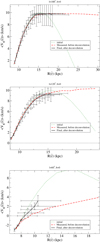	Fig. 5. As in Fig. 4 but with initial velocity $V_R(\mathrm{km}{\mathrm{s}}^{-1})=10sin(1.5\times [\sqrt{R/(1\mathrm{kpc})}-\sqrt{R_{\odot }/(1\mathrm{kpc})]})$.
In the text

	Fig. 6. Monte Carlo simulation of Vϕ. Horizontal error bars indicate the rms value of the mean deconvolved R (thus the indicated value is an average over that range of dispersion). The three panels are for the directions in the plane ℓ = 180°, ℓ = 120° and ℓ = 60°, respectively.
In the text

	Fig. 7. Monte Carlo simulation of Vz. Horizontal error bars indicate the rms value of the mean deconvolved R (thus the indicated value is an average over that range of dispersion). The three panels are for the directions in the plane ℓ = 180°, ℓ = 120° and ℓ = 60°, respectively.
In the text

Fig. 8. Left panels: three components (radial, azimuthal, and vertical, from top to bottom, respectively) of the Galactocentric velocity Median(V) as a function of $X(\overline{r})$ and $Y(\overline{r})$ (X, Y with deconvolution correction according to Sect. 3.1). Application for Gaia-DR2 data including νr measurement with the constraints: |b|< 10°, $\frac{\pi }{\mathrm{\Delta }\pi }>1$. Inner green contour represents the region with error equal to 10, 10, and 2 km s−1 for VR, Vϕ, and VZ, respectively. Middle panels: error (in log scale) of V derived from the expansion in the formulae of $\mathrm{\Delta }\overline{r}={\sigma }_{\overline{r}}$ as systematic error and the dispersion of values of νr, μℓ, and μb divided by the root square of the number of points per bin as statistical errors. Right panels: rms value of V (corrected for measurement errors). Data of this figure are available at the CDS.

In the text

Fig. 9. Left panels: three components (radial, azimuthal and vertical, from top to bottom, respectively) of the Galactocentric velocity median (V) as a function of $R=X(\overline{r})$ and $Z(\overline{r})$ (X, Z with deconvolution correction according to Sect. 6). Application for Gaia-DR2 data including νr measurement with the constraints: 160 ° < ℓ< 200°, $\frac{\pi }{\mathrm{\Delta }\pi }>1$. Inner red contour represents the region with error equal to 10 km s−1. Middle panels: error (in log scale) of V derived from the expansion in the formulae of $\mathrm{\Delta }\overline{r}={\sigma }_{\overline{r}}$ as systematic error and the dispersion of values of νr, μℓ, and μb divided by the root square of the number of points per bin as statistical errors. Right panels: rms value of V (corrected for measurement errors). Data of this figure are available at the CDS.

In the text

	Fig. 10. As in Fig. 9 (V(R, Z), its error and rms value) for 120 ° < ℓ< 160°. Data of this figure are available at the CDS.
In the text

	Fig. 11. As in Fig. 9 (V(R, Z), its error and rms value) for 200 ° < ℓ< 240°. Data of this figure are available at the CDS.
In the text

	Fig. 12. As in Fig. 9 (V(R, Z), its error and rms value) for −20 ° < ℓ<  + 20°. Data of this figure are available at the CDS.
In the text

	Fig. 13. Radial Galactocentric velocity median as a function of $Y(\overline{r})$ for different $X(\overline{r})$ (ΔX = 0.5 kpc) within |b|< 10°.
In the text

Fig. 14. Azimuthal Galactocentric velocity median as a function of $Z(\overline{r})$ for different cuts of constant and $R=X(\overline{r})$ (ΔX = 0.2 kpc) (top panel) or as a function of $R=X(\overline{r})$ for different cuts of $Z(\overline{r})$ (bottom panel). Application for Gaia-DR2 data including νr measurement with the constraints: −20 ° < ℓ< 20° (only top panel) or 160 ° < ℓ< 200°, $\frac{\pi }{\mathrm{\Delta }\pi }>1$.

In the text

	Fig. 15. Vertical Galactocentric velocity median as a function of $\varphi (\overline{r})$ for different Galactocentric radii (ΔR = 0.5 kpc) within |b|< 10°.
In the text

	Fig. 16. As in Fig. 8, this time introducing a correction to the zero-point bias of parallaxes πc = π + 0.03 mas. Data of this figure are available at the CDS.
In the text

References

- Ak, S., Bilir, S., Karaali, S., Buser, R., & Cabrera-Lavers, A. 2007, New Astron., 12, 605 [NASA ADS] [CrossRef] [Google Scholar]
- Antoja, T., Helmi, A., Romero-Gómez, M., et al. 2018, Nature, 561, 360 [NASA ADS] [CrossRef] [Google Scholar]
- Arenou, F., Luri, X., Babusiaux, C., et al. 2018, A&A, 616, A17 [Google Scholar]
- Astraatmadja, T. L., & Bailer-Jones, C. A. L. 2016, ApJ, 832, 137 [NASA ADS] [CrossRef] [Google Scholar]
- Bahcall, J. N., & Soneira, R. M. 1980, ApJS, 44, 73 [NASA ADS] [CrossRef] [Google Scholar]
- Bailer-Jones, C. A. L., Rybizki, J., Fouesneau, M., Mantelet, G., & Andrae, R. 2018, ApJ, 158, 58 [Google Scholar]
- Balázs, L. G. 1995, Inverse Prob., 11, 731 [NASA ADS] [CrossRef] [Google Scholar]
- Bobylev, V. V., & Bajkova, A. T. 2010, MNRAS, 408, 1788 [NASA ADS] [CrossRef] [Google Scholar]
- Bond, N. A., Ivezić, Z., Sesar, B., et al. 2010, ApJ, 716, 1 [NASA ADS] [CrossRef] [Google Scholar]
- Bovy, J., Allende Prieto, C., Beers, T. C., et al. 2012, ApJ, 759, 131 [NASA ADS] [CrossRef] [Google Scholar]
- Bovy, J., Rix, H.-W., Schlafly, E. F., et al. 2016, ApJ, 823, 30 [NASA ADS] [CrossRef] [Google Scholar]
- Carrillo, I., Minchev, I., Kordopatis, G., et al. 2018, MNRAS, 475, 2679 [NASA ADS] [CrossRef] [Google Scholar]
- Casagrande, L., Schönrich, R., Asplund, M., et al. 2011, A&A, 530, A138 [NASA ADS] [CrossRef] [EDP Sciences] [Google Scholar]
- Chen, B., Stoughton, C., Smith, J. A., et al. 2001, ApJ, 553, 184 [NASA ADS] [CrossRef] [Google Scholar]
- Craig, I. J. D., & Brown, J. C. 1986, Inverse Problems in Astronomy (Bristol, UK: Adam Hilger) [Google Scholar]
- Cropper, M., Katz, D., Sartoretti, P., et al. 2018, A&A, 616, A5 [NASA ADS] [CrossRef] [EDP Sciences] [Google Scholar]
- Dias, W. S., & Lépine, J. R. D. 2005, ApJ, 629, 825 [NASA ADS] [CrossRef] [Google Scholar]
- Fang, T.-M., Shei, S.-S., Nagem, R. J., & Sandri, G. V. H. 1994, Il Nuovo Cimento B, 109, 83 [NASA ADS] [CrossRef] [Google Scholar]
- Gaia Collaboration (Prusti, T., et al.) 2016, A&A, 595, A1 [NASA ADS] [CrossRef] [EDP Sciences] [Google Scholar]
- Gaia Collaboration (Brown, A. G. A., et al.) 2018a, A&A, 616, A1 [NASA ADS] [CrossRef] [EDP Sciences] [Google Scholar]
- Gaia Collaboration (Katz, D., et al.) 2018b, A&A, 616, A11 [NASA ADS] [CrossRef] [EDP Sciences] [Google Scholar]
- Galazutdinov, G., Strobel, A., Musaev, F. A., Bondar, A., & Krelowski, J. 2015, PASP, 127, 126 [NASA ADS] [CrossRef] [Google Scholar]
- Golubov, O., Just, A., Bienaymé, O., et al. 2013, A&A, 557, A92 [NASA ADS] [CrossRef] [EDP Sciences] [Google Scholar]
- Hayden, M. R., Bovy, J., Holtzman, J. A., et al. 2015, ApJ, 808, 132 [NASA ADS] [CrossRef] [Google Scholar]
- Haywood, M., Di Matteo, P., Lehnert, M., Katz, D., & Gómez, A. 2013, A&A, 560, A109 [NASA ADS] [CrossRef] [EDP Sciences] [Google Scholar]
- Jupp, D. L. B., & Vozoff, K. 1975, Geophys. J. R. Astron. Soc., 42, 957 [CrossRef] [Google Scholar]
- Juric, M., Ivezic, Z., Brooks, A., et al. 2008, ApJ, 673, 864 [NASA ADS] [CrossRef] [MathSciNet] [Google Scholar]
- Kafle, P. R., Sharma, S., Lewis, G. F., & Bland-Hawthorn, J. 2012, ApJ, 761, 98 [NASA ADS] [CrossRef] [Google Scholar]
- Katz, D., Sartoretti, P., Cropper, M., et al. 2018, A&A, accepted [arXiv:1804.09372] [Google Scholar]
- Kawata, D., Baba, J., Ciuca, I., et al. 2018, MNRAS, 479, L108 [NASA ADS] [CrossRef] [Google Scholar]
- Lindegren, L., Hernández, J., Bombrun, A., et al. 2018, A&A, 616, A2 [NASA ADS] [CrossRef] [EDP Sciences] [Google Scholar]
- Liu, C., Tian, H. J., & Wan, J. C. 2017, IAU Symp., 321, 6 [NASA ADS] [Google Scholar]
- López-Corredoira, M. 2014, A&A, 563, A128 [NASA ADS] [CrossRef] [EDP Sciences] [Google Scholar]
- López-Corredoira, M., & González-Fernández, C. 2016, AJ, 151, 165 [NASA ADS] [CrossRef] [Google Scholar]
- López-Corredoira, M., & Molgó, J. 2014, A&A, 567, A106 [NASA ADS] [CrossRef] [EDP Sciences] [Google Scholar]
- López-Corredoira, M., Hammersley, P. L., Garzón, F., Simonneau, E., & Mahoney, T. J. 2000, MNRAS, 313, 392 [NASA ADS] [CrossRef] [Google Scholar]
- López-Corredoira, M., Abedi, H., Garzón, F., & Figueras, F. 2014, A&A, 572, A101 [NASA ADS] [CrossRef] [EDP Sciences] [Google Scholar]
- Lucy, L. B. 1974, AJ, 79, 745 [NASA ADS] [CrossRef] [Google Scholar]
- Lucy, L. B. 1994, A&A, 289, 983 [NASA ADS] [Google Scholar]
- Lury, X., Brown, A. G. A., Sarro, L. M., et al. 2018, A&A, 616, A9 [NASA ADS] [CrossRef] [EDP Sciences] [Google Scholar]
- Masry, E., & Rice, J. A. 1992, Can. J. Stat., 20, 9 [CrossRef] [Google Scholar]
- Mateu, C., Vivas, A. K., Downes, J. J., & Briceño, C. 2011, Rev. Mex. Astron. Astrofis., 40, 245 [Google Scholar]
- Poggio, E., Drimmel, R., Lattanzi, M. G., et al. 2018, MNRAS, 481, L21 [NASA ADS] [CrossRef] [Google Scholar]
- Polido, P., Jablonski, F., & Lépine, J. 2013, ApJ, 778, 32 [NASA ADS] [CrossRef] [Google Scholar]
- Reid, M. J., Menten, K. M., Brunthaler, A., et al. 2014, ApJ, 783, 130 [Google Scholar]
- Reylé, C., Marshall, D. J., Robin, A. C., & Schultheis, M. 2009, A&A, 495, 819 [NASA ADS] [CrossRef] [EDP Sciences] [Google Scholar]
- Rong, J., Buser, R., & Karaali, S. 2001, A&A, 365, 431 [NASA ADS] [CrossRef] [EDP Sciences] [Google Scholar]
- Sartoretti, P., Katz, D., Cropper, M., et al. 2018, A&A, 616, A6 [NASA ADS] [CrossRef] [EDP Sciences] [Google Scholar]
- Schönrich, R., Binney, J., & Dehnen, W. 2010, MNRAS, 403, 1829 [NASA ADS] [CrossRef] [Google Scholar]
- Siebert, A., Famaey, B., Minchev, I., et al. 2011, MNRAS, 412, 2026 [NASA ADS] [CrossRef] [Google Scholar]
- Soubiran, C., Jasniewicz, G., Chemin, L., et al. 2018, A&A, 616, A7 [NASA ADS] [CrossRef] [EDP Sciences] [Google Scholar]
- Stassun, K. G., & Torres, G. 2018, ApJ, 862, 61 [NASA ADS] [CrossRef] [Google Scholar]
- Tian, H.-J., Liu, C., Wan, J.-C., et al. 2017, Rev. Astron. Astrophys., 17, 114 [Google Scholar]
- Turchin, V. F., Kozlov, V. P., & Malkevich, M. S. 1971, Sov. Phys. Usp., 13, 681 [Google Scholar]
- Ulmer, W. 2010, Inverse Prob., 26, 085002 [NASA ADS] [CrossRef] [Google Scholar]
- Ulmer, W. 2013, J. Phys. Conf. Ser., 410, 012122 [CrossRef] [Google Scholar]
- Wang, H., López-Corredoira, M., Carlin, J. L., & Deng, L. 2018, MNRAS, 477, 2858 [NASA ADS] [CrossRef] [Google Scholar]
- Widrow, L. M., Gardner, S., Yanny, B., Dodelson, S., & Chen, H.-Y. 2012, ApJ, 750, L41 [NASA ADS] [CrossRef] [Google Scholar]
- Williams, M. E. K., Steinmetz, M., Binney, J., et al. 2013, MNRAS, 436, 101 [NASA ADS] [CrossRef] [Google Scholar]
- Xu, Y., Newberg, H. J., Carlin, J. L., et al. 2015, ApJ, 801, 105 [NASA ADS] [CrossRef] [Google Scholar]
- Zinn, J. C., Pinsonneault, M. H., Huber, D. C., & Stello, D. 2018, ApJ, submitted [arXiv:1805.02650] [Google Scholar]