| Issue |
A&A
Volume 708, April 2026
|
|
|---|---|---|
| Article Number | A324 | |
| Number of page(s) | 14 | |
| Section | Planets, planetary systems, and small bodies | |
| DOI | https://doi.org/10.1051/0004-6361/202557580 | |
| Published online | 22 April 2026 | |
Revised entropy of the AQUA equation of state
1
Institute of Space Research, German Aerospace Center (DLR),
Rutherfordstr. 2,
12489
Berlin,
Germany
2
Institut für Physik, Universität Rostock,
Albert-Einstein Str. 23–24,
18051
Rostock,
Germany
3
Observatoire de la Côte d’Azur, Université Côte d’Azur,
96 Boulevard de l’observatoire,
06300
Nice,
France
★ Corresponding author. This email address is being protected from spambots. You need JavaScript enabled to view it.
Received:
7
October
2025
Accepted:
11
March
2026
Abstract
Context. Water is a key constituent of the ice giants Uranus and Neptune, and potentially of Neptune-sized exoplanets. Understanding their present structure and evolution requires knowledge of the equation of state (EoS) and the entropy of the main constituents. Therefore, the EoS and entropy of water are crucial ingredients to ice giant models. The AQUA EoS was constructed to span a wide pressure-temperature (P–T) range by combining several existing water EoSs for different phases. However, one of the EoSs within AQUA contained a mistake in the equation used to compute the entropy.
Aims. We aim to provide a revised AQUA EoS that includes the entropy based on the revised equation. As the region of revised entropies covers the superionic regime, we also aim to improve AQUA in that phase by including further published absolute entropies and internal energies of superionic water derived from DFT-MD simulations and advanced post-processing.
Methods. We defined regions where entropy, density, and internal energy are interpolated whenever a continuous phase transition or no phase transition between the different EoS sources is expected to occur; otherwise, we allowed for jumps in entropy when a first-order phase transition is expected. We ensured a monotonic behaviour in entropy with pressure along isotherms and with temperature along isobars in the revised area of AQUA’s P–T space.
Results. We find that the entropies between the revised and original AQUA differ by up to ±10% in the regions relevant to the deep interiors of adiabatic Neptune-sized planets. The entropy in superionic water is found to be offset with respect to the neighbouring fluid phase by about −10%, which we take as evidence of a first-order phase transition with an associated latent heat release. Ice giant interiors are up to ~650 K colder and the latent heat could partially power the luminosity of Neptune.
Key words: equation of state / planets and satellites: interiors / planets and satellites: physical evolution
© The Authors 2026
 Open Access article, published by EDP Sciences, under the terms of the Creative Commons Attribution License (https://creativecommons.org/licenses/by/4.0), which permits unrestricted use, distribution, and reproduction in any medium, provided the original work is properly cited.
This article is published in open access under the Subscribe to Open model. This email address is being protected from spambots. You need JavaScript enabled to view it. to support open access publication.
1 Introduction
An accurate water equation of state (EoS) that covers a wide range of pressure-temperature conditions and provides the entropy (or thermodynamic parameters) that enable the computation of adiabats is critical in modelling water-rich planets. AQUA (Haldemann et al. 2020) is such an EoS. It combines several EoSs for water in different phases into a single table spanning 0.1 Pa to 400 TPa and 100 to 105 K. Since its release, AQUA has been widely used in the planetary sciences community. Examples include modelling a water-rich layer in the warm Neptune GJ 436b (Guzmán-Mesa et al. 2022) or in sub-Neptunes in the TOI-1260 system (Lam et al. 2023), the TOI-1117 system (Lockley et al. 2025), or in super-Earths (Rodrigues et al. 2025). Other applications include the study of habitability conditions of cold super-Earths (Mol Lous et al. 2022), phase separation in Uranus and Neptune (Cano Amoros et al. 2024), evolution models of Jupiter with fuzzy cores and helium immiscibility (Tejada Arevalo et al. 2025), and the radius gap in the context of the formation of planets with steam and supercritical water-rich atmosphere (Nielsen et al. 2025).
Adiabaticity is a widely used first-order assumption. Even when there are clear hints from the observational side that the temperature profile may deviate from adiabaticity, the adiabatic case serves as the reference state. Planets may also not be fully homogeneous in composition, but have a layered structure with sharp or gradual transitions between layers of constant composition. Moreover, these layers may undergo temporal changes in their composition as a result of demixing upon cooling. A notable example is the iron core formation in terrestrial planets (McCammon et al. 1983), He-rain due to H/He demixing in cool gas giants (Stevenson & Salpeter 1977; Fortney & Hubbard 2003; Nettelmann et al. 2015; Howard et al. 2024), or the water-rain out due to H2/H2O demixing in cool Neptune-sized planets (Bailey & Stevenson 2021; Cano Amoros et al. 2024; Howard et al. 2025).
Along an adiabatic profile, entropy is constant, whereas the pressure, temperature, and density change. The pressure-temperature (P–T) paths of constant entropy can be calculated from thermodynamic relations if the employed EoS provides the density, ρ(P, T), and internal energy, U(P, T).
However, if the planet cools over time, it loses heat, via δq = T(m) ds(m) dm, per mass shell, dm. Direct computation of the heat requires knowledge of the entropy, s(m), at least up to some constant offset, s0. The offset is cancelled out when the difference, ds, is computed. Alternatively, the heat can be calculated from the first law of thermodynamics, dU = δQ − P dV. Here again, offsets in the specific internal energy, u0, are cancelled out. The offsets, u0, will inevitably be there because only energy differences are measurable physical quantities.
The cancellation of energy and entropy offsets holds if the local composition remains constant over time (i.e. homogeneous evolution). However, processes such as rain-out, core erosion, and diffusion lead to local compositions that change over time. In this case of inhomogeneous evolution, the cancellation of energy offset still holds, whereas computing the heat δq directly from entropy requires knowledge of the absolute entropy. The AQUA EoS (Haldemann et al. 2020) provides the specific entropy s(P, T) of water.
AQUA includes data from Mazevet et al. (2019) in the warm, dense matter regime. In addition to their density functional theory-molecular dynamics (DFT-MD) simulations, they draw on multiple sources: in the fluid and superionic region from French et al. (2009), and at high pressures and temperatures from Thomas-Fermi-molecular dynamics (TF-MD) data. Mazevet et al. (2019, hereafter M19) constructed an analytical fit of the Helmholtz free energy as given in their Eq. (1), where the last term, −TS0 with the constant entropy offset, S0, is introduced to yield agreement with the entropy of water of Soubiran & Militzer (2015) to within 10%. In addition to the free energy, Mazevet et al. (2019) provided thermodynamic properties computed from its derivatives, such as the entropy.
After the publication of the AQUA EoS, Mazevet et al. (2021, hereafter M21), introduced a correction to one of the terms of the free energy parametrisation; specifically, a sign change in Eq. (13) of M19. As a consequence, the value of the constant entropy offset S0 was modified. We note that the mass-radius relationships for wet super-Earths obtained before and after the correction appear indistinguishable (see Fig. 13 in Mazevet et al. (2019, 2021)). However, given the importance of entropy in planetary interior modelling and evolution, we constructed a revised AQUA EoS that includes the revised entropies. We also took the opportunity to include the absolute entropy and internal energy values of SI water from DFT-MD simulations and advanced post-processing by French et al. (2016, hereafter F16), instead of relying on thermodynamic integration, which smears out phase transitions.
In this paper, we present a water EoS table that we call revised AQUA. It differs from the original AQUA in terms of the specific entropy s(P, T), density ρ(P, T), internal energy u(P, T), and adiabatic gradient.
The paper is organised as follows. In Sect. 2, we describe the entropy data from F16 and how the different EoS sources were merged into a large-scale table. In Sect. 3 we present the resulting entropy, entropy differences, density, internal energy, and adiabatic gradient over the wide pressure and temperature range. In Sect. 4, we discuss the implications for planet interiors and evolution. The conclusion in Sect. 5 is followed by an appendix where we illustrate the interpolation between different EoS sources.
2 Methods
Our revised AQUA EoS involves two main updates to the original AQUA EoS of Haldemann et al. (2020, hereafter Hal20). First, the revised AQUA includes revised entropy values from M21 in the liquid, supercritical, and superionic (SI) regimes, and second, it includes data in the SI phase from F16. As in the case of the original version of AQUA, the revised AQUA EoS employs additional water EoSs from different sources. They cover different regions of the phase diagram and are listed in Table 1. We refer the reader to Hal20 for details on the EoSs numbered 1, 2, 3, 4, and 6.
Figure 1a shows the water phase diagram over the entire P − T range covered by the EoS sources, guided by Fig. 2 of Hal20. Solid lines show EoS boundaries, which may coincide with physical phase transitions. Dashed lines show further physical phase transitions. Purple and pink shaded areas in panel a show the Mazevet et al. (2019, 2021) region and the French et al. (2016) region that contain the revised and new entropy data, respectively. Symbols in Fig. 1a indicate the subset of data used to define each region. Figure 1b shows the complete set of DFT-MD and TF-MD simulation data for each water phase from Mazevet et al. (2019, 2021) and French et al. (2016).
The Mazevet et al. (2019) EoS was built by ensuring smooth transitions to the Wagner & Pruß (2002) EoS in region 4 in terms of pressure and internal energy. It also covers the low-temperature part of the fluid, molecular phase region, where in the original AQUA, data from Brown (2018) were applied. Since we recovered the smooth transition between the new M21 data and region 4, we saw no advantage to including the data from Brown (2018); therefore, we omitted them in the revised AQUA.
To connect the EoSs that cover different regions of the phase space, interpolations and extrapolations were applied. Haldemann et al. (2020) used two different methods. Their method 1 was applied when a phase transition occurred according to experimental data or the Gibbs free energy potentials; in this case, they switched abruptly all variables at the phase boundary. Discontinuities at expected first-order phase transitions were recovered. Method 2 was used when no phase transition occurs between two different EoS sources and, therefore, the density and entropy would transition smoothly. In this case, Hal20 introduced an interpolation region to ensure a smooth transition.
Regions where we applied interpolation and extrapolation for our revised AQUA are shown in Fig. 1a in grey and green, respectively. For the case when no first-order phase transition is expected between EoSs, we applied cubic Hermite splines, as implemented in the Python package SciPy (Virtanen et al. 2020), which ensures the continuity of the interpolated functions and their first derivatives at the endpoints of the interpolation interval. The location and extent of the interpolation regions were ‘heuristically determined’ to ensure a consistent monotonic behaviour both along isotherms and isobars. These regions, shown in grey, are explained in more detail in Sects. 2.1 and 2.2. The splines were applied along isotherms only. Wherever we interpolated the entropy, the density and internal energy were also interpolated. Examples of the interpolating splines applied to isotherms can be found in Appendix A. The region of extrapolation is explained in Sect. 2.3.
Our approach of ensuring monotonic behavior (∂s/∂T)P ≥ 0 and (∂s/∂P)T ≤ 0 is the following. The first partial derivative is the specific heat at constant pressure, cp = T(∂s/∂T)P with cp > cv. We are not aware of a material where experiments would indicate a negative specific heat capacity. Therefore, ensuring (∂s/∂T)P ≥ 0 is a physically sound choice. The partial derivative (∂S/∂P)T equals −(∂V/∂T)P and, thus, (∂s/∂P)T = 1/Tρ αT with the thermal expansion coefficient αT = −(d ln ρ/d ln T)P. Usually, but not always, αT > 0; for example, in the region of pressure-driven dissociation, the αT of H2 can become negative (Preising et al. 2023). Dissociation also occurs in water at temperatures above ~1500 K and pressures above ~1 kbar, but over an extended range. We did not see signs of negative αT in any individual EoS and we considered it unlikely that this would occur coincidentally in the regions of interpolation. Therefore, we imposed (∂s/∂P)T ≤ 0.
We also note that the CEA package used to obtain the data of region 6 is valid only up to 2 · 104 K (Gordon & McBride 1994; McBride & Gordon 1996). This limit is shown by a vertical dotted line in Fig. 1a. Although Mazevet et al. (2019) provided data from simulations up to 5 · 104 K, the original AQUA extended up to 105 K. We decided to cut the revised AQUA table at 6 · 104 K to limit the amount of extrapolated data. We caution that data in region 6 beyond 2 · 104 K and data in region 7 beyond 5 · 104 K rely on extrapolations.
Water equations of state sources used to construct revised AQUA.
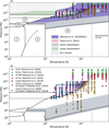 |
Fig. 1 (a) Phase diagram of the revised AQUA with the numbered EoS sources listed in Table 1. Symbols show the simulation results from Mazevet et al. (2019) and French et al. (2016) used in each of the two new regions, 7 and 5, respectively. Region 7, Mazevet et al. (2019, 2021), is shown in purple and region 5, French et al. (2016), in pink. The grey shaded areas show interpolation regions. The green region denotes an area where data from region 3 were linearly extrapolated. Negative or out-of-bounds entropies are shown by the hatched area. The vertical dotted line at 2 · 104 K shows the temperature limit above which region 6 data are extrapolated in both the original and the revised AQUA. The phase boundary between regions 7 and 5 was obtained from Fig. 1 in Redmer et al. (2011) and Fig. 4 in F16. The small boundary between region 5 and region 3 was also taken from F16, marking the boundary between SI water and ice. The dashed line indicating the phase transition from liquid to SI regime in region 7 was taken from F16 up to 1013 Pa and from M19 for higher pressures. (b) High-P, high-T region showing the entire set of pressure and temperature simulation points of F16 in the SI regime (blue and cyan diamonds) and from Mazevet et al. (2019, 2021) in the liquid, SI regimes, and based on Thomas-Fermi data (circles and squares). The black solid lines show EoS boundaries from Hal20 except those around the new region where French et al. (2016) data have been used (see main text for details). |
2.1 Region 7 (entropy revision from M21)
A Fortran routine to produce the EoS table with the revised entropy from the free energy model of M19 is available1. It takes the temperature and density as input and outputs (among other quantities) the pressure, free energy, internal energy, and entropy.
We used this routine to obtain the revised entropy values for each (T, ρ)-combination in AQUA. The (T, ρ) in the original AQUA EoS extends from 102 to 105 K and from 10−10 to 105 kg m−3, both with 100 log-spaced points per order of magnitude.
We substituted the previous entropy values with the revised ones and inspected the intersections with adjacent EoSs. When transitioning from region 4 (gas, liquid and supercritical fluid) to region 7, no phase transition is expected to occur. However, when plotting entropy against pressure, we observed a shift in the isotherms at the 4-to-7 transition. Where the original AQUA had a smooth transition, we found the M21 isotherms would all lie below the corresponding region 4 isotherms. Connecting these two regions at 109 Pa would have yielded a non-physical, downward entropy discontinuity. Moreover, the difference between isotherms was not constant. The coldest isotherm in this region of interest (300 K) had the smallest difference in entropy between regions 4 and 7. We therefore took this isotherm as reference and calculated the necessary shift to ensure a smooth transition at 109 Pa and that would preserve monotonicity for warmer isotherms. We found that a single shift of +425 J/(kg K) applied to the M21 entropies satisfies these criteria. This shift is within the 10% uncertainty on the entropy constant (9.8kBNat) by which Mazevet et al. (2021) shifted their entropy values. After applying the entropy shift, we defined interpolation regions for isotherms crossing different EoS sources. To this end, we split the P − T space as detailed below. We note that even though we are describing the interpolation regions in order of increasing temperatures, this does not represent the order in which we made the decision on the extent of the interpolation regions between neighboring EoSs. In particular, our choice of the optimised extent of the transition from region 6 to 7, described below, influences the choice of the other interpolation regions.
For T ∈ [300–345] K, we interpolated the entropy along isotherms crossing from region 4 to region 3 in the pressure range, P ∈ [5.8 · 108 − P4-to-3] Pa, where P4-to-3(T) = 5.061. 10−4 T4.971. For T ∈ [345–1200] K, isotherms transition from region 4 to region 7 to region 3. Over a very narrow temperature range of T ∈ [345–354] K, isotherms crossing from region 4 to 7 are interpolated across P ∈ [5.8 · 108−2 · 109] Pa. Once in region 7, the transition to the ice VII phase occurs at P4-to-3(T). This narrow range of temperature was necessary to avoid overlap between isotherms.
For T ∈ [354–1000] K and the transition from region 4 to 7, we applied the interpolation across P ∈ [5.8 · 108−2 · 109] Pa. For T > 354 K, the transition between region 7 and region 3 is defined by the melting pressure Pmelt of ice-VII (Hal20):
![Mathematical equation: $\[\log _{10} P_{\text {melt}}=\exp~ \left[x_1 \cdot(T / c)^{x_2}+x_3 \cdot(T / c)^{-1}+x_4 \cdot(T / c)^{-3}\right]-1,\]$](/articles/aa/full_html/2026/04/aa57580-25/aa57580-25-eq1.png) (1)
(1)
where Pmelt is in Pa, c = 355 K, x1 = 2.6752, x2 = −0.0269, x3 = −0.46234, and x4 = 0.1237 (see Table 2 and Eq. (23) in Hal20). For T > 1000 K, we define the interpolation area from region 6 to region 7 according to Eq. (27) of Hal20,
![Mathematical equation: $\[P_{6 \text {-to-7 }}=0.05 ~\mathrm{GPa}+(3 ~\mathrm{GPa}-0.05 ~\mathrm{GPa}) \frac{T / 1000 \mathrm{~K}-1}{39},\]$](/articles/aa/full_html/2026/04/aa57580-25/aa57580-25-eq2.png) (2)
(2)
where P6-to-7 is in Pa.
Using the original AQUA interpolation range from 1–3. P6-to-7 would result in non-monotonic entropy behavior along several isotherms. Non-monotonicity was observed to be just more pronounced with the shift applied to M21 data. We therefore progressively increased the width of the interpolation region; extending it to 0.6–38 · P6-to-7 yields a fully monotonic behaviour for all isotherms that go from region 6 to the new values of region 7. We stress that we aimed, first, to ensure a smooth behavior because no first-order phase transition was expected to occur between regions 6 and 7; second, to ensure monotonicity as, otherwise, a non-monotonic behavior could cause problems when entropy is inverted in planet interior modelling.
For isotherms crossing from the liquid state in region 7 to the SI region 5, we adopted the fluid–SI phase boundaries in Fig. 1 of Redmer et al. (2011) and Fig. 4 of F16. We denote this boundary as P7-to-5. Isotherms in the range T ∈ [1350–11 741] K that cross this boundary display a clear entropy discontinuity.
For temperatures beyond 12 000 K, the fluid–SI phase boundary of F16 flattens when pressures have reached 1013 Pa. However, according to Mazevet et al. (2019, 2021), the fluid-SI transition extends to higher pressures and temperatures, as shown by the dashed line in region 7 in Fig. 1. There, in region 7, the fluid-SI transition appears continuous in entropy at these high temperatures and high pressures due to the parametrisation of the free energy by Mazevet et al. (2019).
2.2 Region 5: (superionic phase from F16)
French et al. (2016) used DFT-MD simulations to obtain water EoS data for P(ρ, T) and a specific internal energy, u(ρ, T). A common procedure for deriving the entropy from DFT-MD simulation data is via a Helmholtz free energy (F) model, where the entropy can readily be computed as the partial derivative S = −(∂F/∂T)V. The key challenge with that approach is to obtain F in the first place. A two-dimensional thermodynamic integration can be used to calculate a surface F(T, V) + F0 (Nettelmann et al. 2012), with the constant F0 to be adjusted to a known classical limit. However, while F(T, V) from the DFT-MD simulations is reliable in the warm-dense matter regime but becomes increasingly inaccurate toward lower densities, the opposite holds for the classical limits. Connecting the free energy surfaces from these methods where they become inaccurate could potentially lead to a large uncertainty in F0 and, thus, the derived entropy.
A more robust common approach is to employ coupling-constant integration, where the potential is made to smoothly transition from the warm-dense matter to the reference state via the coupling-constant, λ. That method however is computationally expensive, as the DFT-MD simulations must be run for different interpolating potential energies U(λ) (Militzer 2009; Soubiran & Militzer 2015).
Mazevet et al. (2019) constructed a physically motivated analytic Helmholtz free energy model that they adjusted to the pressures from the DFT-MD and TF-MD simulations at high densities and to the pressures of the Wagner & Pruß (2002) data in the molecular water regime (region 4). With that approach, the information on the SI phase enters the large-scale free energy model via the fit to the local pressures and internal energy.
French et al. (2016) chose a different approach. They calculated the entropy from the spectrum of vibrational modes in the SI bcc or fcc lattices. Those modes can directly be computed by tracking the motions of nuclei in the MD-simulations. F16 also used them to calculate the nuclear quantum corrections to internal and free energy. To relate the oscillation spectrum to entropy, a two-component separation into a solid component (the oxygen ions in the SI lattice) and a gaseous component for the mobile protons was employed. The challenges with this approach lie in the determination of the size, packing fraction, and oscillation modes of the gaseous particles. Finally, by assuming a temperature-dependent Fermi distribution for the occupation of electronic states, the absolute entropy of SI water given a lattice structure could be calculated.
French et al. (2016) then developed a generic ‘ansatz’ for the Helmholtz free energy F(ρ, T) with 36 fit coefficients for each of the bcc and fcc phases, and adjusted it to the pressures and internal values from the DFT-MD simulations. Even though, in their work, emphasis was on determining the phase boundary between bcc and fcc SI water phases, here, we are interested in the entropy. F16 derived the entropy in both phases from their free energy model up to a constant. To determine the respective constants, they utilised the absolute entropy values from their direct method described above.
The P–T space covered by the simulations of F16 is shown as cyan diamonds for bcc and blue diamonds for fcc in Fig. 1. We obtained the boundary between SI and ice phase for T ∈ [1350–2000] K from their Fig. 4. The pink region in Fig. 1a shows the new region 5, where we used the French et al. (2016) EoS for the revised AQUA EoS.
We used a table with density, temperature, pressure, entropy, and internal energy data that Martin French (pers. commun., 2016) derived from the F16 free energy model. To connect these data back to those of M21 at the high pressures end P > 1012 Pa, we defined an interpolation region for isotherms in the range of T ∈ [2000–11 741] K that transition from region 5 back to region 7 across the pressure range P ∈ [2.88 · 1012−4.47 · 1012] Pa.
Hal20 intended to use the F16 data in the original AQUA, but reported difficulties in transitioning to M19. Although it is hard to tell what the exact issue was, we found that connecting M19 data to F16 along the liquid–SI boundary we used would have led to non-monotonic behaviour. With the revised and shifted M21 data, this is no longer a problem.
2.3 Extrapolations and negative entropies
Our region 3 does not exceed temperatures higher than 2000 K or pressures higher than ≈3 · 1011 Pa. In contrast, Hal 20 connected the ice region 3 at pressures above 7 · 1011 Pa to the results of the fit formula from Mazevet et al. (2019), which appear to be an expansion of the SI phase but not of an ice phase. However, under those low temperatures of 2000 K or less and high pressures of ≈3 · 1011 Pa, the phase diagram of F16 indicates the ice-X phase. No information on the prevalent phase at higher pressures is given, but the flat ice X–SI phase boundary suggests a prevalence of an ice phase rather than a SI phase at higher pressures. Therefore, we linearly extrapolate the French & Redmer (2015) ice data toward higher pressures for isotherms between 100 and 2000 K. This extrapolation region is shaded in green in Fig. 1a. There, we extrapolate entropies to higher pressures either until they become negative or, to avoid overlap with higher-T isotherms where water is SI, up to a limit of 3.2 · 1012 Pa. This limit can be appreciated in Figs. 1a and 4, as discussed below.
In this top-left P–T area of crystalline water at very high-P, negative entropies occur in the original AQUA table and in the M21 data. There, and above our imposed 3.2 · 1012 Pa limit, we substitute the negative entropies by ‘−1’ in the revised AQUA entropy column. This region is indicated by the hatched area labeled as ‘no S values’ in Fig. 1a. Furthermore, we detected a non-monotonic behaviour in the original AQUA entropy and density data for isotherms in the temperature range T ∈ [758–891] K around a pressure of 2 · 1010 Pa. We manually modified the few points in this region to ensure the expected monotonic behaviour based on the shape of the curves before and after this small region. An example of these kinks can be seen in Fig. 4b.
2.4 Thermodynamic consistency
As in Hal20, we performed a thermodynamic consistency check of the revised EoS using their Eq. (29),
![Mathematical equation: $\[\Delta_{\text {Th.c. }}=1-\frac{\rho(T, P)^2\left(\frac{\partial S(T, P)}{\partial P}\right)_T}{\left(\frac{\partial \rho(T, P)}{\partial T}\right)_P}.\]$](/articles/aa/full_html/2026/04/aa57580-25/aa57580-25-eq3.png) (3)
(3)
Figure 2 shows that the revised region 7 and the new region 5 conserve thermodynamic consistency to a level of 1% or better. The strongest inconsistencies arise in the interpolation regions and across first-order phase boundaries. This is expected since we did not develop a free energy model, but simply interpolated the thermodynamic quantities of interest across regions of different EoS models. However, free energy construction methods can also be subject to uncertainties. For instance, for a simple thermodynamic integration, independence from the chosen path must be ensured. A two-step process such as that employed by Militzer (2025), in combination with a coupling constant over intermediate energy functionals, might improve the consistency.
As a step forward to mitigate this, Xie et al. (2025) advocate to treat those regions separately first and then making smooth transitions between the different free energy models. They used the recently developed flow-matching method to compute the free energy and its difference between regions that are based on different applied theories. However, implementing their method is beyond the scope of this work.
Another source of inconsistency arises because we computed the derivatives across physical phase boundaries regardless of discontinuities in the entropy or density. A strong inconsistency is also appreciable in the high temperature regime of region 6, where the data is based on extrapolation. This does not appear in Fig. 3 of Hal20 because their x-axis does not extend beyond 30 000 K.
We point out that for the ice-1h phase, we provided a higher number of significant digits to the entropy data than in the original AQUA table. This is because using the original entropy values would result in a zero-valued denominator of Eq. (3) at pressures up to ~104 Pa. We obtained the updated values from the SeaFreeze package (Journaux et al. 2020), which, as in the case of the original AQUA, includes data for the ice-1 h phase of Feistel & Wagner (2006), but with a higher number of significant digits.
2.5 Internal energy
The revised AQUA also includes the internal energy. We updated it in the new region 5 and made adjustments to the surroundings as described below. Hal20 shifted the internal energies of their regions 4 and 7 by +6.32128736 · 105 J/kg and −2.467871264. 106 J/kg, respectively. Their region 7 was connected to their region 5, which no longer occurs in the revised AQUA. The internal energies in M19 are the same as in M21. However, after expanding the P − T coverage of region 7 to connect to region 4 at 109 Pa, keeping the above-mentioned shift for region 7 would result in crossing isotherms near the transition. Since M21 was built to ensure a smooth transition in internal energy to Wagner & Pruß (2002); namely, between regions 4 and 7, we applied the same shift that Hal20 applied on region 4 to our region 7 (i.e., a constant upward shift of +6.32128736 · 105 J/kg). Afterwards, we interpolated the internal energies across the same interpolation regions used for entropy and density.
We updated the internal energies in the new SI region 5 with the data from French et al. (2016). As described by Mazevet et al. (2021), their zero internal energy reference point differs from that of French et al. (2009) and French & Redmer (2015) by a constant of +7.7 · 107 J/kg. Since the data of French et al. (2016) were obtained using the same method, we expect this shift between M21 and F16 to also hold. After connecting M21 to F16 along the fluid-SI boundary, we observed a slightly PT-dependent offset of 7.407 · 107 to 7.901 · 107 J/kg. The origin of this PT-dependence is unknown, but different zero-point energies are likely to be the main source of this difference. We applied a constant shift of +7.486 · 107 J/kg to F16. This value was chosen to minimise the number of grid points where intersections of isotherms would occur. The need to shift the internal energy to connect neighbouring EoSs was also recently noted by Xie et al. (2025).
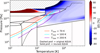 |
Fig. 3 Entropy percentage difference between the revised and the original AQUA EoS (background colors). Negative values (blue-ish) imply higher revised entropies. Coloured lines show adiabatic interior profiles of a Uranus-like planet with upper and lower envelope water abundances of Z1 = 0.360 and Z2 = 0.844, respectively, and surface (1 bar) temperatures of 70,100 and 200 K. Solid and dashed lines indicate adiabatic models computed with the revised and original AQUA, respectively. |
3 Results
In this section, we present the revised AQUA EoS. We show the resulting difference in entropy between the original and the revised EoS, the effect on adiabatic profiles of a Uranuslike planet, and the behaviour of isotherms, isobars, entropy, density, internal energy and adiabatic gradient over the entire pressure–temperature space.
The revised AQUA contains the columns pressure in Pa, temperature in K, density in kg/m3, entropy in J/(kg K), internal energy in J/kg, the derivatives (∂logS/∂logP)T and (∂logS/∂logT)P, the adiabatic gradient, the phase ID, and an interpolation flag. The table can be downloaded from a Zenodo repository2.
3.1 Revised entropies
Figure 3 shows the relative entropy difference Δs(T, P) = sorig.(T, P)/srev.(T, P) − 1 in percentage between the revised and the original AQUA EoS. Negative values imply higher revised entropies. For most of the phase space, the entropy difference stays within ±10%. In region 7, the M21 entropies are higher than those of M19, but lower than the formerly used Brown (2018) data in original AQUA (between ≈ 300 K and 1500 K and 109 Pa and 1010 Pa).
With the entropy shift we applied to the M21 data, the transition between regions 4 and 7 is smooth, while in the original AQUA, an additional region 5 was inserted between 4 and 7 for a smooth transition. Near the transition to region 4, both the revised and original AQUA have similar entropies.
Larger deviations from the original EoS are mostly due to ‘spikes’ in the original AQUA EoS, where entropy rises sharply with pressure along isotherms. As we ensured a monotonic behaviour in s(P, T) and to account for the most likely phase where fit-formula-based entropies appeared to have suspicious values, those spikes do not occur in our revised AQUA. An example is the strong entropy difference around 3 · 1011 Pa; the spike in original AQUA can be seen in Fig. 4b, whereas we linearly extrapolated the curves as shown in Fig. 4a.
3.2 Effect of the revised entropies on an adiabatic ice giant profile
in Fig. 3, we overplotted the adiabatic interior temperature profiles of a Uranus-like planet. As in Cano Amoros et al. (2024), we obtained them using the interior structure code TATOOINE (Baumeister et al. 2020; MacKenzie et al. 2023; Baumeister & Tosi 2023). The underlying planet models assume a three-layer structure with the mass of Uranus, two envelopes of H-He-H2O with a H/He protosolar ratio, and an isothermal rocky core. The upper and lower envelopes have water abundances of Z1 = 0.360 and Z2 = 0.844, respectively. For H and He, we used the EoS from Chabrier & Debras (2021, hereafter CD21). For the core, we used the relation of Hubbard & Marley (1989) for an Earth-like bulk composition. The three P–T profiles are further constrained by 1-bar temperatures T1 bar of 70,100, and 200 K as proxies for the time evolution of an ice giant.
Differences between the solid (based on revised AQUA) and the dashed (based on original AQUA) profiles begin to emerge when the profiles enter region 7, which is where revised and original AQUA differ. For T1 bar = 200 K, the divergence begins at 1000 K and 8.1 · 107 Pa, where the profile is colder until 3.1 · 1011 Pa, and the temperature difference reaches a maximum of −390 K. The profile obtained with the revised AQUA becomes up to 274 K warmer in the central region. For T1 bar = 100 K, the profiles begins to differ at 1000 K and 8.3 · 108 Pa with up to +10 K at 7 · 109 Pa. The revised profile then becomes colder, leading to a maximum difference of −451 K in the central region. For T1 bar = 70 K, the revised profile begins to become warmer at 1 · 109 Pa, with a maximum of +20 K at 1.5 · 1010 Pa, after which it becomes colder than the original profile by up to −654 K in the central region.
For all three cases, the output planet radius (Rp) is slightly smaller when using the revised AQUA. For T1 bar = 200 K, 100 K, and 70 K, the differences are negligible: 0.203%, 0.053% and 0.029%, respectively. The smaller planet radii are due to colder, and thus denser, interior profiles. The small differences are due to the increasing temperature-insensitivity of planet adiabats with pressure in warm dense matter.
The interior models shown in this section are fully adiabatic. However, the interiors for Uranus and Neptune are likely to harbor non-adiabatic regions (Podolak et al. 2019; Tejada Arevalo 2025; Morf & Helled 2025). To construct non-adiabatic ice giant models is beyond the scope of this work.
3.3 Revised entropy along isotherms and isobars
Figures 4 and 5 show examples of entropy profiles along isotherms, while Fig. 6 along isobars. We describe P–T intervals where different phases of water occur, and highlight the major changes with respect to the original AQUA.
3.3.1 Isotherms
The displayed isotherms are divided into three categories: ‘low-T’, ‘mid-T’, and ‘high-T’ for better visibility. The top row of Fig. 4 shows the revised EoS whilst the bottom row shows the original AQUA. The low-T isotherms range from 100 to 800 K. They span several water phases. Isotherms that go from ice-I in region 1 to ice-II, III, -V, -VI in region 2, and then to ice-VII, -VII*, -X in region 3 are characterised by low entropy values, a flat profile within a phase and a jump in entropy at phase transitions. Isotherms that begin at low-P in the gas phase in region 4 have a high entropy that steeply decreases with increasing pressure. These isotherms can pass further through supercritical fluid if past the critical point (green–yellow lines in Fig. 4a), or through liquid water (blue–green lines), or directly into an ice phase (violet lines). In the latter two cases, one can notice the discontinuity due to condensation and sublimation, respectively. Isotherms that remain supercritical pass at around 109 Pa through an interpolation area between regions 4 and 7, before they enter the high-pressure ice VII in region 3, where entropy drops discontinuously. Overall, the first-order phase transitions are clearly visible as discontinuities with respect to pressure. Another example is the perhaps most commonly known liquid-to-ice transition between 109 and 1010 Pa for T < Tcrit.
A comparison of the low-T panels, 4a and 4b, reveals that the strong kink in original AQUA at 2 · 1011 Pa disappears if the entropy in the high-P ice phase X is simply extrapolated in order to adopt a flat behavior as it is known for the low-P ice phases. These spikes resulted from the connection of ice to M19 data above 400 GPa (see Hal20 for details). The M19 data in this region lead to the crossings seen in 4b. To avoid these, we extrapolated the ice data, as explained before. The kinks at temperatures around 800 K and 1010 Pa were also removed, since they were most likely a computational artifact. However, small spikes in the coldest isotherms (from 100 to 254 K) and 5 · 108 Pa remain, as we did not revise or manipulate data in that area.
Figures 4c and 4d show mid-T isotherms ranging from 1000 to 7000 K. Those also reveal discontinuities and changes with respect to the original AQUA. Isotherms between 1320 and 2000 K transition from region 6 to region 7 in the supercritical fluid through the P–T-dependent interpolation region, then pass through a small area of SI water in region 5 around 1011 Pa, and then to ice-X in region 3. The decrease in entropy with pressure is much stronger in SI water than in the ice phases. Simple linear extrapolation can therefore lead to an intersection of isotherms at high pressures. We cut the ice-phase isotherms (purple) at 3.2 · 1012 Pa to avoid any intersection with warmer SI phase isotherms.
Isotherms at T > 2000 K also transition from region 6 to region 7, onto the SI region 5 and further into the SI part of region 7. Figure 4c reveals a new result and a major difference between revised and original AQUA: an entropy jump at the fluid (region 7) to SI (region 5) phase. This occurs around 1011 and 1012 Pa. With ~10%, this entropy jump amounts to about 1000 J/kg K and is of the same magnitude as the transition between SI and high-P ices. This new result can have a large effect on the evolution of an ice-giant-like planet, as will be discussed in Sect. 4. The entropy jump between SI water (region 5) and fluid water (region 7) can also be noticed in the high-T panel of 4e, although only for the coldest isotherms there. Warmer isotherms that cross regions 6, 7, and the SI part of 7 do not show a first-order phase transition.
Furthermore, as our chosen interpolation region between 6 and 7 is wider than in the original AQUA, the transition is less abrupt in Fig. 4e compared to Fig. 4f. This explains the visibly higher entropies for the warmest isotherms.
Figure 5 shows a zoom-in of the isotherms in the range T ∈ [900–14 500] K to highlight the first-order transitions and the consequent entropy jump. Isotherms between 900 and 1200 K (the six lowest curves) transition from the fluid phase of M21 to the ice phase from French & Redmer (2015). The entropy jump varies from ~37% to 42%. Isotherms between 1200 and 2000 K transition from fluid (M21) to SI (F16) to the ice phase (FR15). The SI region spanned by these isotherms is very small (see Fig. 1), and the entropy jump at the fluid-SI transition ranges from ~3% to 10%. The next jump, at the SI-ice transition, ranges from ~26% to 33%. For isotherms between 2000 and 11 700 K, these isotherms transition from fluid (M21) to SI (F16) and then to SI (M21). The entropy jump at the fluid-SI transition is between 10% and 11%, where the biggest jump in magnitude is of 1279 J/(kg K). Toward the critical point, one would expect the temperature gap to close slowly. Within region 5, no such closure is found, suggesting the critical point, if any, occurs at higher temperatures than 11 741 K, i.e. beyond those in region 5. However with the region 5–7 transition at about ~11741 K, the entropy gap disappears abruptly because the M21 data do not contain phase transitions. The drop between 2.88 · 1012 and 4.47 · 1012 Pa in Fig. 5 when transitioning from SI F16 to SI M21 is not a physical feature; it results from the narrow interpolation region between the two EoSs.
Recently, Militzer (2025) obtained similar results in their abinitio calculations of water entropy. He found a jump in entropy and density when transitioning from the fluid to SI regime in the range T ∈ [1000–12 000] K, with a relative entropy jump between ~3% and 8% and a maximum magnitude of 934 J/kg K. A comparison between Militzer (2025) and revised AQUA in the liquid and SI regime can be found in Fig. B.1.
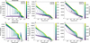 |
Fig. 4 Entropy along isotherms of revised AQUA (top row) and original AQUA (bottom row). The low-T panels (left) show isotherms passing through regions 1, 2, and 3, or through 4, 7, 3 (+ extrapolations of region 3). The mid-T panels (center) show isotherms passing through regions 6, 7, 5, and 7 again. The high-T panels (right) show isotherms crossing regions 6,5 and 7 or just regions 6 to 7 for the highest temperatures. The low-T panel for the original AQUA shows a kink around 1.83 · 1010 Pa for several isotherms around 800 K, and a sudden rise in entropy at 3 · 1011 Pa. Both features have intentionally been removed in the revised AQUA. The numbers on panels a, c, and e indicate the regions of the phase diagram as shown in Fig. 1 crossed by the isotherms. |
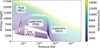 |
Fig. 5 Zoom-in of entropy along isotherms in the range T ∈ [900–14 500] K. The labels show the phases and the EoSs crossed by the isotherms within the pressure range plotted. Jumps in entropy can be observed when first-order phase transitions occur upon connecting EoSs. The warmest isotherms only cross the M21EoS, where the fluid-SI transition appears continuous in entropy. FR15: (French & Redmer 2015). |
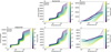 |
Fig. 6 Entropies along isobars of revised AQUA (top row) and original AQUA (bottom row). At low-P (left), we made no changes to the original AQUA data. Low-P isobars cross regions 1, 4, and 6. In the mid-P panel (center), isobars cross regions 1 (or 2), 4, 7, and 6. Isobars in the high-P panel (right) transition through regions 3, 7, and 5. |
3.3.2 Isobars
Figure 6 shows the isobars, with the top row once again showing the isobars from the revised EoS and the bottom row showing those from the original AQUA. In the low-P panel, Fig. 6a, the isobars range from 10−1 to 104 Pa. These isobars transition from ice in region 1 to liquid (or vapor) in region 4 across the melting (or sublimation) curves, into gas in region 6. No changes were made in this low-P region, which is why only the original EoS is shown here.
Applied changes start at 4 · 107 Pa. In the mid-P panels 6b and 6c, isobars at 104 to 109 Pa cross from ice phases in regions 1 and 2 to the liquid state in regions 4 and 7, and end up in the vapor or supercritical fluid phase in regions 4 and 7.
The largest difference with respect to the original AQUA can be seen in the high-P panels 6d and 6e, where isobars range from 3 · 109 Pa to 3 · 1014 Pa. These isobars cross the ice VII or ice X phases in region 3, depending on the pressure, then into the liquid and supercritical fluid in region 7 or the new SI region 5, and then back to the fluid state of region 7. The inclusion of the new region 5 yields well-behaved monotonic isobars, in contrast to the non-monotonic behaviour in that P–T area seen in Fig. 6e.
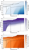 |
Fig. 7 Specific entropy (a), density (b), and specific internal energy (c) of the revised AQUA as a function of pressure and temperature. As in previous figures, the hatched area at high pressure corresponds to the region where entropy values have been cut or are negative. The vertical dotted line at 2 · 104 K delimits the boundary after which CEA data are extrapolated. |
3.4 Maps of entropy, density, internal energy, and adiabatic gradient
Figures 7a, 7b and 7c show maps of entropy, density, and internal energy. The entropy revision from M21 also affects the adiabatic gradient, which is an important parameter for the determination of the temperature profile in convective regions of planets, for the computation of the radiative-to-convective boundary based on the Schwarzschild criterion, and for the strength of compositional mixing and heat loss. Figure 8 shows the adiabatic gradient from the revised AQUA table. The gradient was calculated from the relation,
![Mathematical equation: $\[\nabla_{\mathrm{ad}}=\left(\frac{\partial \log T}{\partial \log P}\right)_S=-\frac{\left(\frac{\partial \log S}{\partial \log P}\right)_T}{\left(\frac{\partial \log S}{\partial \log T}\right)_P}.\]$](/articles/aa/full_html/2026/04/aa57580-25/aa57580-25-eq4.png) (4)
(4)
After revising entropy in the EoS table, we calculated its derivative with respect to pressure (temperature), along constant temperature (pressure). Unsurprisingly, these numerical derivatives were not smooth along first-order phase transitions. Therefore, similar to the entropy and density, the derivatives were also interpolated across phase boundaries using cubic splines. The values of these smoothened derivatives, which we used to calculate the adiabatic gradient, are also provided in the table.
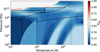 |
Fig. 8 Adiabatic temperature gradient of the revised AQUA as a function of temperature and pressure. The black lines denote the boundaries, same as in Fig. 1. |
4 Discussion
4.1 Latent heat of superionic water
An important finding of this work is an entropy discontinuity at the fluid-to-SI water transition that is associated with a strong latent heat of the order of 10% of absolute entropy for the concerned isotherms. It is known that a transition to a more ordered phase can lead to a discontinuity in the entropy. This is also seen in the transition from liquid in region 7 (previously region 5) to ice in region 3. We did not detect a critical point because if there were any, we would expect it to occur in region 7.
However, the circumstance that we have applied a shift to the entropy in region 7 raises the question of how substantial the evidence of the entropy difference between fluid and SI water actually is. The original and revised versions of AQUA both contain the absolute entropies of ice phases VII and X from French & Redmer (2015) (region 3). Revised AQUA includes the absolute entropies of SI water from French et al. (2016) (region 5). The absolute entropies from these two sources were derived by the same method (see Sect. 2.2). We are not aware of an inconsistency between these two data sources. Therefore, we rely on the assumption that they are consistent. If unaccounted-for entropy offsets exist, they could only result from transitions between regions 3 and 4 and between 4 and 7. Also even without the shift on the M21 entropies, a jump would be present, but simply smaller in magnitude.
The absolute entropies in region 4 are adjusted to the zero-point entropy at T0 = 0 K of ice-1 h of 189.13 J/kg K (Haldemann et al. 2020). The absolute entropies in region 3 make use of a fit formula that adopts s0 = 0 at the zero-point T0 = 0 K and are derived for ice VII, whereas in cold water, a structural change to ice VIII would occur with a small but finite zero-point entropy. Without an overlap in the PT-range where the same crystal structure and thus the same zero-point entropy applies, it is not possible to accurately quantify a possible difference in the absolute entropy between regions 4 and 3. At present, there is no indication of such an unintentional offset between regions 3 and 4.
We determined an entropy shift of +425 J/kg K between regions 4 and 7 that would bring both data sources into an optimal agreement. This shift is well within the uncertainty of the entropy constant of M21, but it may have itself an uncertainty. By visual inspection, the uncertainty should be less than ±5 J/kg K, which is 0.5% of the entropy jump between fluid and SI water. Therefore, we believe that regions 4 and 7 are consistent, and so should be all of regions 3, 4, 5, and 7. We conclude that there is no evidence of the entropy jump at the fluid-to-SI phase transition to be non-real, but it clearly has an uncertainty that we estimate to be much less than the height of the jump, although hard to quantify precisely. We interpret the jump in specific entropy seen in Fig. 4 as a latent heat, qL(P, T) = TΔsSI.
4.2 Temperatures in ice giants with a superionic core
It is important to know the temperatures in the deep interior of the ice giants in order to understand how and where their magnetic field is generated, what their bulk composition is, and how their present structure links to the early stage of planet formation. According to Fig. 3, the revised AQUA predicts slightly lower temperatures in the deep interiors of the ice giants today than the original AQUA. This may suggest that carbon, which is expected to be abundant in the ice giants interiors (Hubbard 1981; Ali-Dib et al. 2014), separates out earlier from the oxygen-hydrogen system, either because of direct carbon-immiscibility in water (Militzer 2024) or because of more favourable conditions for diamond formation with lower temperature (Kraus et al. 2017), and that the ice-giant magnetic field morphology may have been established earlier in their history. These planet adiabats are also useful for estimating whether or not, locally, the medium would be convective or stably stratified.
However, an uncertainty persists about the transition to the SI phase as it may not occur at constant entropy. When a SI core freezes and if the fluid-SI phase transition is first-order (as is the case in revised AQUA) latent heat will be released. Therefore, the entropy in the SI phase will be lower than in the fluid phase. The temperature at the top of the mass shell in the planet that undergoes this phase transition will adjust to the temperature of the fluid phase, and the temperature profile in the mass shell will adopt an adiabatic profile defined by this boundary condition. As a result, the temperatures in the mass shell that transitioned from fluid to SI will be lower than along a constant-entropy adiabat. This continuous-temperature transition, instead of continuous-entropy is the classical approach of treating discontinuous phase transitions, such as at the Earth’s upper mantle-lower mantle transition (Brown & Shankland 1981). Constant-entropy adiabats instead follow for a while the (steeper) phase boundary and therefore, exhibit a steeper temperature gradient, as can be seen in Fig. 3. Such behaviour is also suggested for the olivine to wadsleyite transition at the bottom of the Earth’s upper mantle (Katsura 2022; Li et al. 2025).
For later stages, it is not clear whether the SI core can cool quick enough to adjust to the low temperatures of the mass shell that has frozen lastly. If not, a thermal boundary layer will develop as proposed for ice giant models with a freezing core (Stixrude et al. 2021; James & Stixrude 2024). In that case, the temperatures in the planet in the SI phase will fall between those with full energy release and the ones of Fig. 3 without latent heat release. Still, the core temperatures will be lower than with the original AQUA, and the planet radius differences will slightly increase compared to the ones given in Sect. 3.2 due to the lower temperatures.
4.3 Evolution of ice giants with a superionic core
It is important to understand the evolution of the ice giants because it links the present-day structure with the early stage of their formation and the formation of the solar system as a whole. Here, we estimate the influence of the latent heat on the thermal evolution of Neptune. We ran the evolution calculation based on Neptune adiabats at different 1 bar temperatures and for two different EoS combinations: the revised AQUA together with CD21 for H/He, and H2O-REOS with REOS. 3 for H/He. For the first EoS combination, we computed the evolution using a newly developed evolution code written in python, which is now part of the TATOOINE framework. It follows the same approach as MOGROP (Nettelmann et al. 2012), and was benchmarked against it. The latter code was used in combination with the REOS-based Neptune model. Details of the model do not matter except for the Z2 = 0.84 (0.8) water mass fraction in the inner envelope for the two different EoS-combinations. The evolution model provides the interior structure (mass, m, pressure, P, temperature, T) and energy balance (effective luminosity, L, equilibrium luminosity, Leq, intrinsic luminosity, Lint) over time, t. The transition to the SI phase is found for each temporary structure by comparing the interior P–T profiles with the fluid-SI phase boundary TSI(P). When an intersection is found, the mass ![Mathematical equation: $\[m_{S I}^{i}\]$](/articles/aa/full_html/2026/04/aa57580-25/aa57580-25-eq5.png) is noted. The mass of the shell that freezes over the time interval dt = ti+1 − ti is
is noted. The mass of the shell that freezes over the time interval dt = ti+1 − ti is ![Mathematical equation: $\[d m=\left(m_{S i}^{i+1}-m_{S I}^{i}\right)\]$](/articles/aa/full_html/2026/04/aa57580-25/aa57580-25-eq6.png) , out of which Z2 × dm is water. The latent heat that is released from that mass shell is
, out of which Z2 × dm is water. The latent heat that is released from that mass shell is ![Mathematical equation: $\[\delta Q_{L}^{i}=Z_{2} ~d m \times T\left(m^{i}\right) \Delta s_{S I}\]$](/articles/aa/full_html/2026/04/aa57580-25/aa57580-25-eq7.png) . It yields the contribution LQ = δQL/dt to the intrinsic luminosity,
. It yields the contribution LQ = δQL/dt to the intrinsic luminosity, ![Mathematical equation: $\[L_{\text {int}}=4 \pi R_{p}^{2} ~\sigma_{\mathrm{B}} T_{\text {int}}^{4}\]$](/articles/aa/full_html/2026/04/aa57580-25/aa57580-25-eq8.png) , where σB is Boltzmann constant.
, where σB is Boltzmann constant.
The evolution of Lint is provided by the evolution model as Lint(t) = L(t) − Leq(t), where the total luminosity L(t) is derived from Rp(t) and T1 bar(t) while ![Mathematical equation: $\[L_{\text {eq}}(t)=4 \pi R_{p}^{2}(1- \left.A_{B}\right) f^{-1} ~C_{\text {sol}}(t)(a / 1 ~\mathrm{AU})^{-2}\]$](/articles/aa/full_html/2026/04/aa57580-25/aa57580-25-eq9.png) . Here, we have the solar constant
. Here, we have the solar constant ![Mathematical equation: $\[C_{\text {sol}}=\sigma_{\mathrm{B}} T_{\text {Sun}}^{4}(t)\left(R_{\text {Sun}}(t) / 1 ~\mathrm{AU}\right)^{2}\]$](/articles/aa/full_html/2026/04/aa57580-25/aa57580-25-eq10.png) and assumed Bond Albedo AB = 0.3.
and assumed Bond Albedo AB = 0.3.
The onset of core freezing depends on the interior temperature of the planet, which itself is EoS-dependent. Our Neptune profiles computed with the revised AQUA are colder than those with REOS. They cross the fluid-SI boundary when T1 bar ≲ 156 K, while when T1 bar ≲ 88 K with REOS. Figure 9 shows the influence of including the latent heat in the evolution. The models without the latent heat effect underestimate the observed Lint by 6% (revised AQUA) and 14% (REOS). With the revised AQUA, the latent heat effect contributes 10–35% to Lint and delays the thermal evolution by 0.6–0.7 Gyr. With REOS, the effect contributes 15–24% and the delay is 0.3–0.4 Gyr. These results suggest that the inclusion of latent heat can provide at least a significant part of the missing luminosity source to explain the brightness of Neptune.
However, we may have overestimated the intrinsic luminosity of the baseline model. First, we assumed AB = 0.3 as measured by Voyager, while post-Voyager observations of Jupiter and Saturn revised their albedoes upward, for Jupiter from 0.35 to 0.5. Second, we neglected angular momentum conservation, which would have further reduced the predicted luminosity. Therefore, other effects might play a role.
While we would expect a similar behaviour for Uranus, a comparative study of Uranus and Neptune is beyond the scope of this work. Nevertheless, may we conclude that the presence of an additional heat source in Uranus would strengthen the picture that Uranus is not fully adiabatic, as adiabatic models already overestimate its luminosity. Clearly, we would require advanced thermal evolution models based on revised AQUA EoS and that not only include the effect from thermal boundary layers and SI core freezing self-consistently (Scheibe et al. 2021; James & Stixrude 2024), but also account for phase separation between water and hydrogen (Cano Amoros et al. 2024; Howard et al. 2025) and of carbon in HCON-mixtures.
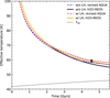 |
Fig. 9 Thermal evolution of an adiabatic Neptune model using the revised AQUA without the latent heat effect (dashed blue) and with the latent heat (dashed red), and using the H2O-REOS without and with latent heat (black and yellow solid lines, respectively). The black symbol shows Neptune’s present-day effective temperature (Teff) and the dotted line shows the evolution of the equilibrium temperature (Teq) for an albedo of 0.3. |
4.4 Not the last water EoS
With the availability of DFT-MD simulations thanks to increasing computational capabilities, the water EoS has been improved in accuracy, especially in the warm dense matter regime as evidenced by the good agreement with experimental Hugoniot data (Knudson et al. 2012). Although our revised AQUA implements DFT-MD-based data via the M21 EoS source, it is unlikely to represent the final large-scale water EoS development.
In this work, we ensured the matching of different water EoSs. However, a given EoS may still be incorrect – even if its free energy functional was constructed to be thermodynamically consistent. Once appropriate shifts and interpolation regions were defined, the EoS matching proved straightforward. Nevertheless, the thermodynamic consistency check reveals the largest deviations precisely across the interpolation regions, suggesting that these regions may also expose intrinsic deficiencies of the individual EoSs.
DFT-MD methods suffer from a major source of uncertainty: the choice of the exchange-correlational (xc) functional. The revised AQUA includes DFT-MD data based on the PBE functional; however, alternative xc-functionals are known to yield different pressures and internal energies. For hydrogen, Cozza et al. (2026) tested 18 × xc functionals and reported relative deviations in pressure of up to ±20% between the PBE and SCAN functionals. This would not be relevant if SCAN (and variants thereof) would not show the lowest deviation (5% in P, 15% in U) when benchmarked against what they consider to be the most accurate method, which is QMC. Consequently, a water EoS constructed from SCAN-based data could yield significantly different pressures, internal energies and thus entropies compared to revised AQUA, with deviations exceeding the uncertainties introduced by our EoS matching procedure.
On the other hand, Jupiter has for decades been regarded as the reference planet for testing our understanding of the H/He EoSs. For QMC- or SCAN-based hydrogen EoSs, these tests indicate that the predicted densities are too high (equivalently, pressures too low) to be consistent with Jupiter’s radius and gravity field (Cozza et al. 2026). The revised AQUA will like-wise face similar tests against future water EoSs constructed with other xc functionals.
5 Conclusion
The widely used water EoS AQUA (Haldemann et al. 2020) contains entropies in the warm dense matter regime that were later found to be erroneous due to a sign-error in the Free energy model used to generate them (Mazevet et al. 2019, 2021).
In this work, we have revised AQUA, providing the entropy, density, internal energy, and adiabatic gradient on a P–T grid. It differs from the original AQUA in four aspects. First, it includes the revised entropies of Mazevet et al. (2021); second, it includes the absolute entropies and internal energies of SI water from French et al. (2016). Third, and as a consequence, the interpolation regions between different EoS sources have been adjusted. We set them to be large enough to ensure a monotonic behaviour in S(T, P). Fourth, at high pressures and low temperatures (T < 2000 K) where theoretical or experimental guidance is missing, the ice-X phase is assumed to prevail instead of SI water. This assumption raises the entropy to positive values. Otherwise, for even higher pressures, we provided no data for this area. In case of known first-order phase transitions, we allowed for a jump in entropy and density. As a result, the revised and original AQUA exhibit several major differences between them, with a potentially large influence on interior models of ice giants. Our main findings are as follows:
We obtained a smooth transition between the entropies of Wagner & Pruß (2002) and Mazevet et al. (2021) after applying an upward shift of the latter by ~425 J/(kg K);
Along ice giant adiabats, the entropy difference between original and revised AQUA is within 10%, with higher revised entropies leading to up to 650 K colder deep interiors. By construction, the entropy difference is zero for pressures below ~0.1 GPa, but can increase substantially where values are based on extrapolations, especially in the region of high-pressure ice;
We see strong evidence to support a first-order phase transition between the fluid and the SI phase with a magnitude of ~1000 J/kg K, which is ~10% of the absolute values.
The accompanying latent heat release upon interior cooling could power the luminosity of Neptune.
Given that AQUA is one of several large-scale water EoSs, following earlier ones such as QEOS (More et al. 1988), ANEOS (Thompson 1990), Sesame 7150 (Lyon & Johnson 1992), and H2O-REOS (Nettelmann et al. 2008), its revised version contributes to a continuously advancing field. We anticipate further refinements of AQUA. For instance, while the underlying PBE-exchange-correlation functional-based DFT-MD data show an excellent agreement with experimental data (Mazevet et al. 2021), other functionals, such as HSE or SCAN, may yield different entropies in unprobed regions of the phase space. We also note that further important physical properties of water for planetary modelling, such as electrical and thermal conductivities and viscosity, should also be included in future water tables.
Water is a key component in the modelling of ice giants and volatile-rich Neptune-sized or sub-Neptune exoplanets, but such studies also require large-scale EoS tables, complete with entropy, for other important substances such as methane and ammonia. These are crucial for enabling thermal evolution modelling that accounts for compositional changes due to phase separation. Finally, the development of self-consistent thermal evolution models is necessary to accurately incorporate the effect of latent heat release when a SI core undergoes freezing.
Data availability
The table can be downloaded from the Zenodo repository at https://doi.org/10.5281/zenodo.18609452.
Acknowledgements
We thank Armin Bergermann for constructive discussions on the water EoS. MCA and NT acknowledge the support of the German Science Foundation (DFG) through the research unit FOR 2440 “Matter under planetary interior conditions” (projects PA 3689/1-1 and NE 1734/2-2). NN acknowledges support through DFG-grant NE 1734/3-1. We acknowledge discussions within the PLATO Exoplanet Science Work-Packages 116.100 and 116.200.
References
- Ali-Dib, M., Mousis, O., Petit, J.-M., & Lunine, J. I. 2014, ApJ, 793, 9 [NASA ADS] [CrossRef] [Google Scholar]
- Bailey, E., & Stevenson, D. J. 2021, PSJ, 2, 64 [Google Scholar]
- Baumeister, P., & Tosi, N. 2023, A&A, 676, A106 [NASA ADS] [CrossRef] [EDP Sciences] [Google Scholar]
- Baumeister, P., Padovan, S., Tosi, N., et al. 2020, ApJ, 889, 42 [Google Scholar]
- Brown, J. M. 2018, Fluid Phase Equilib., 463, 18 [Google Scholar]
- Brown, J., & Shankland, T. 1981, Geophys. J. Int., 66, 579 [Google Scholar]
- Cano Amoros, M., Nettelmann, N., Tosi, N., Baumeister, P., & Rauer, H. 2024, A&A, 692, A152 [NASA ADS] [CrossRef] [EDP Sciences] [Google Scholar]
- Chabrier, G., & Debras, F. 2021, ApJ, 917, 4 [NASA ADS] [CrossRef] [Google Scholar]
- Cozza, C., Nakano, K., Howard, S., et al. 2026, Phys. Rev. Res., 8 [Google Scholar]
- Feistel, R., & Wagner, W. 2006, J. Phys. Chem. Ref. Data, 35 [Google Scholar]
- Fortney, J. J., & Hubbard, W. B. 2003, Icarus, 164, 228 [NASA ADS] [CrossRef] [Google Scholar]
- French, M., & Redmer, R. 2015, Phys. Rev. B, 91, 014308 [CrossRef] [Google Scholar]
- French, M., Mattsson, T. R., Nettelmann, N., & Redmer, R. 2009, Phys. Rev. B, 79, 054107 [NASA ADS] [CrossRef] [Google Scholar]
- French, M., Desjarlais, M. P., & Redmer, R. 2016, Phys. Rev. E, 93, 022140 [Google Scholar]
- Gordon, S., & McBride, B. J. 1994, Tech. rep., NASA Lewis Research Center [Google Scholar]
- Guzmán-Mesa, A., Kitzmann, D., Mordasini, C., & Heng, K. 2022, MNRAS, 513, 4015 [CrossRef] [Google Scholar]
- Haldemann, J., Alibert, Y., Mordasini, C., & Benz, W. 2020, A&A, 643, A105 [NASA ADS] [CrossRef] [EDP Sciences] [Google Scholar]
- Howard, S., Müller, S., & Helled, R. 2024, A&A, 689, A15 [NASA ADS] [CrossRef] [EDP Sciences] [Google Scholar]
- Howard, S., Helled, R., Bergermann, A., & Redmer, R. 2025, A&A, 703, A154 [NASA ADS] [CrossRef] [EDP Sciences] [Google Scholar]
- Hubbard, W. B. 1981, Science, 214, 145 [Google Scholar]
- Hubbard, W., & Marley, M. S. 1989, Icarus, 78, 102 [NASA ADS] [CrossRef] [Google Scholar]
- James, D., & Stixrude, L. 2024, SSRv, 220, 21 [Google Scholar]
- Journaux, B., Brown, J. M., Pakhomova, A., et al. 2020, J. Geophys. Res. Planets, 125, e2019JE006176 [Google Scholar]
- Katsura, T. 2022, JGR: Solid Earth, 127, e2021JB023562 [Google Scholar]
- Knudson, M., Desjarlais, M., Lemke, R., et al. 2012, Phys. Rev. Lett., 108, 091102 [Google Scholar]
- Kraus, D., Vorberger, J., Pak, A., et al. 2017, Nat. Astron., 1, 606 [NASA ADS] [CrossRef] [Google Scholar]
- Lam, K. W. F., Cabrera, J., Hooton, M. J., et al. 2023, MNRAS, 519, 1437 [Google Scholar]
- Li, R., Dannberg, J., Gassmöller, R., Lithgow-Bertelloni, C., & Stixrude, L. 2025, Geochem. Geophys. Geosyst., 26, e2024GC011600 [Google Scholar]
- Lockley, I. S., Armstrong, D. J., Fernández Fernández, J., et al. 2025, MNRAS, 541, 919 [Google Scholar]
- Lyon, S., & Johnson, J. 1992, Los Alamos National Laboratory [Google Scholar]
- MacKenzie, J., Grenfell, J. L., Baumeister, P., et al. 2023, A&A, 671, A65 [NASA ADS] [CrossRef] [EDP Sciences] [Google Scholar]
- Mazevet, S., Licari, A., Chabrier, G., & Potekhin, A. Y. 2019, A&A, 621, A128 [NASA ADS] [CrossRef] [EDP Sciences] [Google Scholar]
- Mazevet, S., Licari, A., Chabrier, G., & Potekhin, A. Y. 2021, arXiv e-prints [arXiv:1810.05658v2] [Google Scholar]
- McBride, B. J., & Gordon, S. 1996, Tech. rep., NASA Lewis Research Center [Google Scholar]
- McCammon, C. A., Ringwood, A. E., & Jackson, I. 1983, Lunar Planet. Sci. Conf., 88, 501 [Google Scholar]
- Militzer, B. 2009, J. Phys. A Math. Theor., 42, 214001 [Google Scholar]
- Militzer, B. 2024, PNAS, 121, e2403981121 [Google Scholar]
- Militzer, B. 2025, ApJ, 990, 20 [Google Scholar]
- Mol Lous, M., Helled, R., & Mordasini, C. 2022, Nat. Astron., 6, 819 [NASA ADS] [CrossRef] [Google Scholar]
- More, R. M., Warren, K. H., Young, D. A., & Zimmerman, G. B. 1988, Phys. Fluids, 31, 10 [Google Scholar]
- Morf, L., & Helled, R. 2025, A&A, 704, A183 [NASA ADS] [CrossRef] [EDP Sciences] [Google Scholar]
- Nettelmann, N., Holst, B., Kietzmann, A., et al. 2008, ApJ, 683, 1217 [NASA ADS] [CrossRef] [Google Scholar]
- Nettelmann, N., Becker, A., Holst, B., & Redmer, R. 2012, ApJ, 750, 52 [NASA ADS] [CrossRef] [Google Scholar]
- Nettelmann, N., Fortney, J. J., Moore, K., & Mankovich, C. 2015, MNRAS, 447, 3422 [NASA ADS] [CrossRef] [Google Scholar]
- Nielsen, J., Johansen, A., Bali, K., & Dorn, C. 2025, A&A, 695, A184 [NASA ADS] [CrossRef] [EDP Sciences] [Google Scholar]
- Podolak, M., Helled, R., & Schubert, G. 2019, MNRAS, 487, 2653 [NASA ADS] [CrossRef] [Google Scholar]
- Preising, M., French, M., Mankovich, C., Soubiran, F., & Redmer, R. 2023, ApJS, 269, 47 [NASA ADS] [CrossRef] [Google Scholar]
- Redmer, R., Mattsson, T. R., Nettelmann, N., & French, M. 2011, Icarus, 211, 798 [CrossRef] [Google Scholar]
- Rodrigues, J., Barros, S. C. C., Santos, N. C., et al. 2025, A&A, 695, A237 [NASA ADS] [CrossRef] [EDP Sciences] [Google Scholar]
- Scheibe, L., Nettelmann, N., & Redmer, R. 2021, A&A, 650, A200 [NASA ADS] [CrossRef] [EDP Sciences] [Google Scholar]
- Soubiran, F., & Militzer, B. 2015, ApJ, 806, 228 [NASA ADS] [CrossRef] [Google Scholar]
- Stevenson, D. J., & Salpeter, E. E. 1977, ApJS, 35, 239 [NASA ADS] [CrossRef] [Google Scholar]
- Stixrude, L., Baroni, S., & Grasselli, F. 2021, PSJ, 2, 222 [Google Scholar]
- Tejada Arevalo, R. 2025, ApJ, 989, L40 [Google Scholar]
- Tejada Arevalo, R., Sur, A., Su, Y., & Burrows, A. 2025, ApJ, 979, 243 [Google Scholar]
- Thompson, S. L. 1990, ANEOS analytic equations of state for shock physics codes input manual, Tech. rep., Sandia National Labs [Google Scholar]
- Virtanen, P., Gommers, R., Oliphant, T. E., et al. 2020, Nat. Methods, 17, 261 [Google Scholar]
- Wagner, W., & Pruß, A. 2002, J. Phys. Chem. Ref. Data, 31, 387 [Google Scholar]
- Xie, H., Howard, S., & Mazzola, G. 2025, Phys. Rev. Res., 7, L032028 [Google Scholar]
Appendix A Construction of isotherms
Figures A.1 to A.4 show examples of the construction of isotherms across different EoS boundaries. Entropy is plotted against pressure. The various lines show the original AQUA isotherm (solid), the revised isotherm from Mazevet et al. (2021)(dashed), and (when applicable) the isotherm based on the French et al. (2016) data (dotted). Red lines show where the cubic splines were applied to ensure a smooth and monotonic behaviour. The brown lines show extrapolation of the isotherms. Finally, the grey lines show the final, revised isotherms.
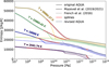 |
Fig. A.1 Construction of isotherms around the fluid-to-SI transition for temperatures between 2000 K and 6 · 104 K. Isotherms for T > 2000 K cross from region 6 to region 7 through an interpolation region ranging from 0.6·P6-to7 Pa to 38·P6-to-7 Pa. Across the interpolation region, a cubic spline (shown in red) was used to connect the original AQUA isotherm (solid lines) to the new data from Mazevet et al. (2021) (dashed lines) with the +425 J/(kg K) shift applied. The 2041.74 K and 10000 K follow the Mazevet et al. (2021) data until the boundary between region 7 and region 5 is met. For the 2041.74 K case, this occurs at 6.08 · 1010 Pa. For the 10000 K isotherm, this is at 1.40 · 1012 Pa. At these pressures, the isotherms stop following the Mazevet et al. (2021) data and begin following French et al. (2016) (dotted lines). This occurs up to 2.88 · 1012 Pa, where a new spline until 4.47 · 1012 Pa is applied to transition from French et al. (2016) back to Mazevet et al. (2021). Isotherms at 33884.42 K and 58884.37 K simply have the spline showing the transition from region 6 to 7 applied, and then continue following Mazevet et al. (2021). The grey curves show the final, revised isotherms. |
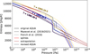 |
Fig. A.2 Construction of isotherms around the fluid-to-SI to ice X transition for temperatures between 1320 K and 2000 K. Isotherms cross from region 6 to region 7 through an interpolation region ranging from 0.6·P6-to7 Pa to 38·P6-to-7 Pa. Across the interpolation region, a cubic spline (shown in red) was used to connect the original AQUA isotherm (solid lines) to the new data from Mazevet et al. (2021) (dashed lines) with the +425 J/(kg K) shift applied. The isotherms follow the Mazevet et al. (2021) data until the boundary between region 7 and region 5 is met. For the 1380.38 K isotherm, the Mazevet et al. (2021) data is followed until 5.09 · 1010 Pa. Then the isotherm will follow the French et al. (2016) data (dotted line), which will lead to an expected discontinuity, and until 6.04 · 1010 Pa where region 5 will finish. Then the isotherm will go from following French et al. (2016) to following the original AQUA data again, also leading to an expected but much larger discontinuity. After 3 · 1011 Pa, the ice will be extrapolated linearly. This extrapolation is shown in brown and will be cut at 3.2 · 1012 Pa in the final table. For the 1659.59 K, the transition from Mazevet et al. (2021) to French et al. (2016) occurs at 5.48 · 1010 Pa and the transition from French et al. (2016) back to the original AQUA at 8.47 · 1010 Pa. For the 1995.26 K, the isotherm follows Mazevet et al. (2021) after the spline until 6 · 1010 Pa and then French et al. (2016) until 1.25 · 1011 Pa, after which it goes back to the original AQUA and then extrapolation (brown lines). The grey curves show the final, revised isotherms. |
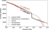 |
Fig. A.3 Construction of isotherms around the fluid-to-ice X transition for temperatures between 1200 K and 1320 K. Isotherms cross from region 6 to region 7 through an interpolation region ranging from 0.6·P6-to7 Pa to 38·P6-to7 Pa. Across the interpolation region, a cubic spline (shown in red) was used to connect the original AQUA isotherm (solid lines) to the new data from Mazevet et al. (2021) (dashed lines) with the +425 J/(kg K) shift applied. These isotherms follow Mazevet et al. (2021) after the spline until the boundary between region 7 and region 3 is met, which occurs at 4.49 · 1010 Pa for 1202.26 K and at 5.12 · 1010 Pa for 1318.26 K. After that boundary, the isotherms follow the original AQUA again up to 3 · 1011 Pa and then the linear extrapolation (brown lines). The grey curves show the final, revised isotherms. |
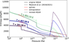 |
Fig. A.4 Construction of isotherms around the liquid- and supercritical-to-ice VII transition for temperatures between 300 K and 1000 K. Isotherms within this range cross from region 4 to region 7 through an interpolation region from 5.8 · 108 Pa to 2 · 109 Pa, except the 301.99 K case which goes up to P4-to-3 (the boundary marking the transition from region 4 to ice VI in region 2). Across the interpolation region, a cubic spline (shown in red) was used to connect the original AQUA isotherm (solid lines) to the new data from Mazevet et al. (2021) (dashed lines) with the +425 J/(kg K) shift applied. After the spline, the Mazevet et al. (2021) data is followed by the isotherms at 457.98, 851.14 until the boundary between region 7 and region 3 is met, which occurs at 3.53 · 109 Pa, 2.23 · 1010 Pa. After this boundary, the original AQUA is followed again until 3 · 1011 Pa, after which the isotherms are linearly extrapolated (brown lines). The grey curves show the final, revised isotherms. |
Appendix B Comparison to Militzer 2025
Militzer (2025) recently published ab-initio calculations of water in the liquid and SI fcc phase employing the thermodynamic integration method. We compare the entropy from that EoS along isotherms with that revised AQUA in Fig. B.1, which shows Militzer (2025) also finds an offset in the entropy when transitioning from liquid to superionic.
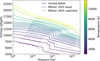 |
Fig. B.1 Isotherms of revised AQUA EoS (solid lines) in the liquid and SI regime compared to the EoS results from ab initio simulations by Militzer (2025) (dashed and dotted for liquid and SI, respectively). |
All Tables
All Figures
|
Fig. 1 (a) Phase diagram of the revised AQUA with the numbered EoS sources listed in Table 1. Symbols show the simulation results from Mazevet et al. (2019) and French et al. (2016) used in each of the two new regions, 7 and 5, respectively. Region 7, Mazevet et al. (2019, 2021), is shown in purple and region 5, French et al. (2016), in pink. The grey shaded areas show interpolation regions. The green region denotes an area where data from region 3 were linearly extrapolated. Negative or out-of-bounds entropies are shown by the hatched area. The vertical dotted line at 2 · 104 K shows the temperature limit above which region 6 data are extrapolated in both the original and the revised AQUA. The phase boundary between regions 7 and 5 was obtained from Fig. 1 in Redmer et al. (2011) and Fig. 4 in F16. The small boundary between region 5 and region 3 was also taken from F16, marking the boundary between SI water and ice. The dashed line indicating the phase transition from liquid to SI regime in region 7 was taken from F16 up to 1013 Pa and from M19 for higher pressures. (b) High-P, high-T region showing the entire set of pressure and temperature simulation points of F16 in the SI regime (blue and cyan diamonds) and from Mazevet et al. (2019, 2021) in the liquid, SI regimes, and based on Thomas-Fermi data (circles and squares). The black solid lines show EoS boundaries from Hal20 except those around the new region where French et al. (2016) data have been used (see main text for details). |
| In the text | |
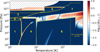 |
Fig. 2 Thermodynamic consistency of the revised AQUA EoS based on Eq. (3). |
| In the text | |
|
Fig. 3 Entropy percentage difference between the revised and the original AQUA EoS (background colors). Negative values (blue-ish) imply higher revised entropies. Coloured lines show adiabatic interior profiles of a Uranus-like planet with upper and lower envelope water abundances of Z1 = 0.360 and Z2 = 0.844, respectively, and surface (1 bar) temperatures of 70,100 and 200 K. Solid and dashed lines indicate adiabatic models computed with the revised and original AQUA, respectively. |
| In the text | |
|
Fig. 4 Entropy along isotherms of revised AQUA (top row) and original AQUA (bottom row). The low-T panels (left) show isotherms passing through regions 1, 2, and 3, or through 4, 7, 3 (+ extrapolations of region 3). The mid-T panels (center) show isotherms passing through regions 6, 7, 5, and 7 again. The high-T panels (right) show isotherms crossing regions 6,5 and 7 or just regions 6 to 7 for the highest temperatures. The low-T panel for the original AQUA shows a kink around 1.83 · 1010 Pa for several isotherms around 800 K, and a sudden rise in entropy at 3 · 1011 Pa. Both features have intentionally been removed in the revised AQUA. The numbers on panels a, c, and e indicate the regions of the phase diagram as shown in Fig. 1 crossed by the isotherms. |
| In the text | |
|
Fig. 5 Zoom-in of entropy along isotherms in the range T ∈ [900–14 500] K. The labels show the phases and the EoSs crossed by the isotherms within the pressure range plotted. Jumps in entropy can be observed when first-order phase transitions occur upon connecting EoSs. The warmest isotherms only cross the M21EoS, where the fluid-SI transition appears continuous in entropy. FR15: (French & Redmer 2015). |
| In the text | |
|
Fig. 6 Entropies along isobars of revised AQUA (top row) and original AQUA (bottom row). At low-P (left), we made no changes to the original AQUA data. Low-P isobars cross regions 1, 4, and 6. In the mid-P panel (center), isobars cross regions 1 (or 2), 4, 7, and 6. Isobars in the high-P panel (right) transition through regions 3, 7, and 5. |
| In the text | |
|
Fig. 7 Specific entropy (a), density (b), and specific internal energy (c) of the revised AQUA as a function of pressure and temperature. As in previous figures, the hatched area at high pressure corresponds to the region where entropy values have been cut or are negative. The vertical dotted line at 2 · 104 K delimits the boundary after which CEA data are extrapolated. |
| In the text | |
|
Fig. 8 Adiabatic temperature gradient of the revised AQUA as a function of temperature and pressure. The black lines denote the boundaries, same as in Fig. 1. |
| In the text | |
|
Fig. 9 Thermal evolution of an adiabatic Neptune model using the revised AQUA without the latent heat effect (dashed blue) and with the latent heat (dashed red), and using the H2O-REOS without and with latent heat (black and yellow solid lines, respectively). The black symbol shows Neptune’s present-day effective temperature (Teff) and the dotted line shows the evolution of the equilibrium temperature (Teq) for an albedo of 0.3. |
| In the text | |
|
Fig. A.1 Construction of isotherms around the fluid-to-SI transition for temperatures between 2000 K and 6 · 104 K. Isotherms for T > 2000 K cross from region 6 to region 7 through an interpolation region ranging from 0.6·P6-to7 Pa to 38·P6-to-7 Pa. Across the interpolation region, a cubic spline (shown in red) was used to connect the original AQUA isotherm (solid lines) to the new data from Mazevet et al. (2021) (dashed lines) with the +425 J/(kg K) shift applied. The 2041.74 K and 10000 K follow the Mazevet et al. (2021) data until the boundary between region 7 and region 5 is met. For the 2041.74 K case, this occurs at 6.08 · 1010 Pa. For the 10000 K isotherm, this is at 1.40 · 1012 Pa. At these pressures, the isotherms stop following the Mazevet et al. (2021) data and begin following French et al. (2016) (dotted lines). This occurs up to 2.88 · 1012 Pa, where a new spline until 4.47 · 1012 Pa is applied to transition from French et al. (2016) back to Mazevet et al. (2021). Isotherms at 33884.42 K and 58884.37 K simply have the spline showing the transition from region 6 to 7 applied, and then continue following Mazevet et al. (2021). The grey curves show the final, revised isotherms. |
| In the text | |
|
Fig. A.2 Construction of isotherms around the fluid-to-SI to ice X transition for temperatures between 1320 K and 2000 K. Isotherms cross from region 6 to region 7 through an interpolation region ranging from 0.6·P6-to7 Pa to 38·P6-to-7 Pa. Across the interpolation region, a cubic spline (shown in red) was used to connect the original AQUA isotherm (solid lines) to the new data from Mazevet et al. (2021) (dashed lines) with the +425 J/(kg K) shift applied. The isotherms follow the Mazevet et al. (2021) data until the boundary between region 7 and region 5 is met. For the 1380.38 K isotherm, the Mazevet et al. (2021) data is followed until 5.09 · 1010 Pa. Then the isotherm will follow the French et al. (2016) data (dotted line), which will lead to an expected discontinuity, and until 6.04 · 1010 Pa where region 5 will finish. Then the isotherm will go from following French et al. (2016) to following the original AQUA data again, also leading to an expected but much larger discontinuity. After 3 · 1011 Pa, the ice will be extrapolated linearly. This extrapolation is shown in brown and will be cut at 3.2 · 1012 Pa in the final table. For the 1659.59 K, the transition from Mazevet et al. (2021) to French et al. (2016) occurs at 5.48 · 1010 Pa and the transition from French et al. (2016) back to the original AQUA at 8.47 · 1010 Pa. For the 1995.26 K, the isotherm follows Mazevet et al. (2021) after the spline until 6 · 1010 Pa and then French et al. (2016) until 1.25 · 1011 Pa, after which it goes back to the original AQUA and then extrapolation (brown lines). The grey curves show the final, revised isotherms. |
| In the text | |
|
Fig. A.3 Construction of isotherms around the fluid-to-ice X transition for temperatures between 1200 K and 1320 K. Isotherms cross from region 6 to region 7 through an interpolation region ranging from 0.6·P6-to7 Pa to 38·P6-to7 Pa. Across the interpolation region, a cubic spline (shown in red) was used to connect the original AQUA isotherm (solid lines) to the new data from Mazevet et al. (2021) (dashed lines) with the +425 J/(kg K) shift applied. These isotherms follow Mazevet et al. (2021) after the spline until the boundary between region 7 and region 3 is met, which occurs at 4.49 · 1010 Pa for 1202.26 K and at 5.12 · 1010 Pa for 1318.26 K. After that boundary, the isotherms follow the original AQUA again up to 3 · 1011 Pa and then the linear extrapolation (brown lines). The grey curves show the final, revised isotherms. |
| In the text | |
|
Fig. A.4 Construction of isotherms around the liquid- and supercritical-to-ice VII transition for temperatures between 300 K and 1000 K. Isotherms within this range cross from region 4 to region 7 through an interpolation region from 5.8 · 108 Pa to 2 · 109 Pa, except the 301.99 K case which goes up to P4-to-3 (the boundary marking the transition from region 4 to ice VI in region 2). Across the interpolation region, a cubic spline (shown in red) was used to connect the original AQUA isotherm (solid lines) to the new data from Mazevet et al. (2021) (dashed lines) with the +425 J/(kg K) shift applied. After the spline, the Mazevet et al. (2021) data is followed by the isotherms at 457.98, 851.14 until the boundary between region 7 and region 3 is met, which occurs at 3.53 · 109 Pa, 2.23 · 1010 Pa. After this boundary, the original AQUA is followed again until 3 · 1011 Pa, after which the isotherms are linearly extrapolated (brown lines). The grey curves show the final, revised isotherms. |
| In the text | |
|
Fig. B.1 Isotherms of revised AQUA EoS (solid lines) in the liquid and SI regime compared to the EoS results from ab initio simulations by Militzer (2025) (dashed and dotted for liquid and SI, respectively). |
| In the text | |
Current usage metrics show cumulative count of Article Views (full-text article views including HTML views, PDF and ePub downloads, according to the available data) and Abstracts Views on Vision4Press platform.
Data correspond to usage on the plateform after 2015. The current usage metrics is available 48-96 hours after online publication and is updated daily on week days.
Initial download of the metrics may take a while.