| Issue |
A&A
Volume 638, June 2020
|
|
|---|---|---|
| Article Number | A121 | |
| Number of page(s) | 11 | |
| Section | Planets and planetary systems | |
| DOI | https://doi.org/10.1051/0004-6361/201937376 | |
| Published online | 23 June 2020 | |
The challenge of forming a fuzzy core in Jupiter
1
Center for Theoretical Astrophysics and Cosmology Institute for Computational Science, University of Zürich Winterthurerstrasse 190,
8057
Zürich,
Switzerland
e-mail: This email address is being protected from spambots. You need JavaScript enabled to view it.
2
Department of Physics and McGill Space Institute, McGill University, 3600 rue University,
Montreal,
QC H3A 2T8,
Canada
Received:
20
December
2019
Accepted:
27
April
2020
Abstract
Recent structure models of Jupiter that match Juno gravity data suggest that the planet harbours an extended region in its deep interior that is enriched with heavy elements: a so-called dilute or fuzzy core. This finding raises the question of what possible formation pathways could have lead to such a structure. We modelled Jupiter’s formation and long-term evolution, starting at late-stage formation before runaway gas accretion. The formation scenarios we considered include both primordial composition gradients, as well as gradients that are built as proto-Jupiter rapidly acquires its gaseous envelope. We then followed Jupiter’s evolution as it cools down and contracts, with a particular focus on the energy and material transport in the interior. We find that none of the scenarios we consider lead to a fuzzy core that is compatible with interior structure models. In all the cases, most of Jupiter’s envelope becomes convective and fully mixed after a few million years at most. This is true even when we considered a case where the gas accretion leads to a cold planet, and large amounts of heavy elements are accreted. We therefore conclude that it is very challenging to explain Jupiter’s dilute core from standard formation models. We suggest that future works should consider more complex formation pathways as well as the modelling of additional physical processes that could lead to Jupiter’s current-state internal structure.
Key words: planets and satellites: formation / planets and satellites: interiors / planets and satellites: gaseous planets / planets and satellites: composition / planets and satellites: individual: Jupiter / methods: numerical
© S. Müller et al. 2020
 Open Access article, published by EDP Sciences, under the terms of the Creative Commons Attribution License (http://creativecommons.org/licenses/by/4.0), which permits unrestricted use, distribution, and reproduction in any medium, provided the original work is properly cited.
1 Introduction
The Juno mission (Bolton et al. 2017) recently mapped Jupiter’s gravitational field with high precision (Folkner et al. 2017; Iess et al. 2018). Traditionally, Jupiter’s interior was modelled with a three-layer structure including: (i) a central compact icy and rocky core; (ii) an inner envelope of metallic hydrogen and helium; and (iii) an outer envelope of molecular hydrogen and helium. These models typically assumed an adiabatic temperature profile for the planet, and the distribution of the heavy elements within the envelope(s) was assumed to be constant (e.g. Stevenson 1982; Guillot 2005). New interior structure models that fit the gravitational moments suggest that Jupiter has a dilute or fuzzy core, rather than a compact one (Wahl et al. 2017; Debras & Chabrier 2019). This suggests that there is an extended region in the innermost part of the planet that is highly enriched with heavy elements.
The idea that Jupiter could have heavy-element composition gradients was proposed decades ago (Stevenson 1982, 1985), and there has been an ongoing effort to explore structure models with chemically in-homogenous layers and non-adiabatic interiors (Chabrier & Baraffe 2007; Leconte & Chabrier 2012; Lozovsky et al. 2017; Berardo & Cumming 2017; Vazan et al. 2018; Debras & Chabrier 2019). Recent formation models confirm that giant planets are expected to form with a primordial composition gradient in their deep interiors, but this region is typically more compact than predicted by structure models (Lozovsky et al. 2017; Helled & Stevenson 2017). An interior with a composition gradient could be a result of core erosion (e.g. Guillot et al. 2004; Moll et al. 2017), by which heavy elements from a compact core are dredged upwards. Constraints on the transport properties of heavy elements in hydrogen-helium mixtures suggest that from a chemical point of view, core erosion could operate in Jupiter (Soubiran & Militzer 2016; Soubiran et al. 2017). This also depends crucially on the state of the core. Mazevet et al. (2019a) show that during Jupiter’s history, the constituents that make up Jupiter’s heavy-element core were at least at some point molten, and as such could be either mixed into the envelope or become stably stratified due to semi-convection (e.g. Wood et al. 2013). It is yet to be investigated whether convective mixing can indeed lead to core erosion during Jupiter’s evolution. Semi-convection (or double-diffusive convection) has been proposed to explain that Jupiter could harbor a large composition gradient (Leconte & Chabrier 2012). In this region, the thermally unstable region would not develop large-scale convection due to a stabilising mean molecular weight gradient. In the double-diffusive regime, diffusion of temperature is more efficient than that of composition, and therefore the composition can be stably stratified.
Recent work has focused on investigating whether it is possible that a composition gradient in Jupiter’s envelope is stable against large-scale convection throughout its evolution (Vazan et al. 2018). A particular model that has a large dilute core, and matches some observational constraints was presented. However, the initial model was created ad-hoc and was not based on formation models. This raises a challenging question: what are the possible formation and evolution paths that lead to a dilute core as inferred from structure models of Jupiter?
Here, we followed the formation of Jupiter in the core-accretion framework (Mizuno 1980; Pollack et al. 1996), starting at early times before Jupiter acquired its gaseous envelope. Then, we followed the runaway gas accretion phase and the subsequent evolution, properly accounting for mixing of heavy elements within the planet. This allows us to determine whether a primordial composition gradient could be formed and sustained in Jupiter to explain its fuzzy core, or if other mechanisms must be invoked. We find that forming a fuzzy core in Jupiter, as suggested by recent studies, is challenging in the standard framework for Jupiter’s formation. This paper is structured as follows: in Sect. 2, we give an overview of how we modelled the thermal evolution of Jupiter with MESA (Paxton et al. 2011, 2013, 2015, 2018, 2019), and present the different formation scenarios we considered. In Sect. 3, we present our formation and evolution models, and show that the outer convection zone can quickly grow and mix large parts of the envelope. We show that our results are robust in terms of our model parameters, which include opacity, equation of state, and whether we allow semi-convective mixing in Sect. 3.4. In Sect. 4, we put our results in the context of current interior structure models, and we summarise our findings in Sect. 5.
2 Methods
2.1 The MESA code
We modelled Jupiter’s thermal evolution from late-stage formation until today with the Modules for Experiments in Stellar Astrophysics (MESA) code, release 10 108 (Paxton et al. 2011, 2013, 2015, 2018, 2019) with a modified equation of state following Vazan et al. (2013) (see Sect. 2.2 and Appendix A for details). The code numerically solves the fully coupled 1D structure and evolution equations under hydrostatic equilibrium (Paxton et al. 2011). The equations are solved with the Henyey method (Henyey et al. 1965) on an adaptive Lagrangian grid with the mass coordinate m. Energy transport by radiative diffusion, electron conduction, and convection is included.
The local stability of a radiative layer is calculated with the Ledoux criterion ∇T < ∇ad + (φ∕δ)∇μ, where ∇T = d lnT∕d lnP, ∇ad, and ∇μ = d lnμ∕d lnP are the temperature gradient, adiabatic temperature gradient, and mean molecular weight gradient, respectively, and  and
and  are material derivatives. In radiative regions, ∇T is equal to the radiative temperature gradient ∇rad. In convective regions, the temperature gradient is obtained by solving the cubic mixing-length theory equations (see e.g. Kippenhahn et al. 2012 for details). To avoid partial pressure derivatives that can be numerically noisy, MESA calculates the composition term as a quantity measuring the pressure difference of neighbouring shells due to composition (Paxton et al. 2013). If (φ∕δ) ∇μ > 0, the denser material is below the lighter one, and the composition term is stabilising against convection. In a homogeneous region, ∇μ = 0 and the Ledoux criterion reduces to the standard Schwarzschild criterion. If a region is Ledoux stable but Schwarzschild unstable, a double-diffusive instability (semi-convection) may be present that could lead to additional mixing (Wood et al. 2013; Radko et al. 2014). Apart from in Sect. 3.4, we do not include semi-convection in this work.
In 1D planetary evolution models, convection is commonly treated as a diffusive process with the mixing length recipe, which requires a free parameter αmlt, which, following Vazan et al. (2018), is set to 0.1. For semi-convection, we used the diffusive approximation from Langer et al. (1983, 1985) as implemented in MESA. This recipe also requires a free parameter, which can be interpreted as the height of the double-diffusive layers. The parameter’s value is poorly constrained, and could range over a few orders of magnitude (Leconte & Chabrier 2012).
For the opacity, we used two different sets of tables: in the inner regions, where pressures and temperatures are high, MESA includes the conductive opacity from Cassisi et al. (2007). Although these opacity tables extend into the range relevant to planetary interiors, they were originally developed for stellar interiors, where matter is fully ionised. As a result, the Cassisi et al. (2007) values should be taken with caution (see e.g. Podolak et al. 2019 for discussion). As a result, we investigated the sensitivity of our results on the assumed conductive opacity in Sect. 3.4. For the gas opacity at lower temperatures, we used the tables from Freedman et al. (2008). The Freedman opacity does not include the effect of grains. As a test, we calculated our models including grain opacity using the analytical fit to the Ferguson et al. (2005) dust opacity with an extrapolation for the lower temperature as presented by Valencia et al. (2013). While the detailed evolutionary path and the final interior structure are affected by the inclusion of grains or scaling of the conductive opacity, we find that our general conclusions are unchanged (see Sect. 3.4 for details).
2.2 A planetary equation of state for MESA
While MESA includes the SCvH (Saumon et al. 1995) tables, the equation of state (EoS) implemented in MESA is not applicable for modelling giant planets with heavy-element mass fractions Z > 0. We therefore implemented a modified version of the EoS presented in Vazan et al. (2013) that is suitable for planetary interiors into MESA. Our EoS combines the EoS from Chabrier et al. (2019) for hydrogen and helium and QEoS (More et al. 1988) for water or rock withthe additive volume law to calculate thermodynamic variables for an arbitrary mixture. Details of the implementation are given in Appendix A. While there are more advanced of equations of state for water for planetary interior conditions (French et al. 2009; Mazevet et al. 2019b), they do not cover the temperature-pressure range required for modelling Jupiter’s formation and evolution. In addition, the water EoS we are using was and applied for planetary evolution in previous work (Vazan et al. 2013, 2015, 2016, 2018). In order to make sure that our conclusions are unaffected by the choice of the EoS, we compared the density at a given pressure and temperature for water with QEoS and the EoS from French et al. (2009). We find that the QEoS underestimates the density by ~ 5− 10% in the relevant regime. This difference is significantly smaller than the differences that arise when we assume a different chemical composition for the heavy elements. The sensitivity of our results to the assumed EoS is presented in Sect. 3.4.
2.3 Initial model and runaway gas accretion
We used a modified MESA routine (create_initial_model) to create an initial adiabatic model corresponding to Jupiter at the onset of the runaway accretion phase. At that point, proto-Jupiter has a mass of 58 M⊕ and an entropy S ≃ 8 kB per baryon, which is roughly within the constraints given by formation models of Jupiter (Cumming et al. 2018). The value of the total mass was chosen such that the primordial composition gradient can be extended and isn’t constrained to just a few Earth masses. The initial entropy for proto-Jupiter at the onset of runaway gas accretion depends on the formation model parameters. We purposely chose a low-entropy case in order to build a steep entropy gradient as proto-Jupiter accretes gas, which should suppress convection, and can assist in forming composition gradients.
The composition in the interior was gradually adjusted in a pseudo-evolution (with the relax_initial_composition routine), such that the heavy-element fraction increases towards the centre. Since the true composition gradient of proto-Jupiter is unknown, we created initial models with three different composition gradients. Figure 1 shows the heavy-element distribution in proto-Jupiter before the onset of runaway gas accretion. Hot_compact_Z roughly matches composition profiles from formation models of Jupiter that include planetesimal dissolution (Lozovsky et al. 2017; Helled & Stevenson 2017), which generally leads to a steep gradient. Models Hot/Cold_extended_Z represent proto-Jupiters with a small dilute core that accretes a large amount of heavy elements during runaway gas accretion. The goal of these scenarios is to create a similar composition gradient to the starting model in Vazan et al. (2018), who found that this initial condition can lead to a model of Jupiter that matches Jupiter’s radius and inferred moment of inertia today. In our work, we imposed this composition profile by allowing for the accretion of heavy elements during runaway gasaccretion. This was done by adjusting the composition of the material that is accreted as a function of the growing Jupiter’s mass. In particular, we calculated the heavy-element mass fraction of the accreted gas as  , where M(t) is proto-Jupiter’s mass at time t, while keeping hydrogen-to-helium ratio constant at the proto-solar value, meaning Xproto = 0.705, Yproto = 0.275. The same istrue for the third profile Cold_high_Z, except that it begins with more heavy elements and also accretes a much larger amount. We considered this model in order to explore a formation pathway that leads to significant accretion of heavy elements during runaway. The heavy-element masses before runaway are MZ = 23, 16 and 28 M⊕, respectively. The heavy-element mass that is accreted during runaway is ≃ 10 M⊕ (Hot_compact_Z), ≃ 30 M⊕ (Hot/Cold_extended_Z) and ≃60 M⊕ (Cold_high_Z), respectively.
Recent interior models suggest that the maximum total heavy-element mass in Jupiter is ≃ 45 M⊕. Most of our models exceed this value (see Sect. 3.3). The reason is that the total heavy-element mass depends on the assumed chemical constituents for the “metals”, and our calculations use a pure water EoS. It is therefore clear that our models require a higher heavy-element content. In addition, our models are intentionally high in metals, since we focused on formation scenarios that are favourable to yielding a dilute-core structure.
To model the growth of giant planets during the detached phase, we followed previous work by Berardo & Cumming (2017). During this stage, (for the most part) hydrogen and helium gas falls onto an accretionshock at the planet’s surface (Marleau et al. 2017, 2019). The limiting gas accretion rate Ṁg was calculated using the formula from Lissauer et al. (2009; their Eq. (2)). Once the accretion rate reached a maximum value of either 10−2 M⊕ yr−1 (Hot_compact_Z & Hot_extended_Z) or 10−4 M⊕ yr−1 (Cold_extended_Z & Cold_high_Z), we kept it constant at these values. It is important to properly account for the accretion shock. Previous work (Berardo & Cumming 2017; Cumming et al. 2018) has shown that, depending on the radiative efficiency of the shock, Jupiter could have formed with an extended radiative envelope. We adopted the shock temperature parameter χ of Cumming et al. (2018) that determines the temperature of the newly accreted material. It is zero if the planet’s surface temperature is not affected by the accretion, and unity if the temperature of the accreted material reflects the fact that it is radiating away the accretion energy. In order to investigate the influence of a hot/cold runaway stage, we allowed Hot_compact_Z & Hot_extended_Z to accrete at a maximum rate of 10−2 M⊕ yr−1 with χ = 1, which represents a hot start. In Cold_extended_Z Cold_high_Z we set Ṁmax = 10−4 M⊕ yr−1 and χ = 0, yielding cold starts. The various models are summarised in Table 1. After reaching Jupiter’s mass, runaway gas accretion was stopped, and we followed the long-term planetary evolution and the mixing of heavy elements in the interior.
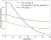 |
Fig. 1 Heavy-element distribution in proto-Jupiter vs. mass at the onset of runaway gas accretion for the different models. The total mass in each model is M = 58 M⊕, and the totalheavy element masses are MZ = 23 (Hot_compact_Z) 16 (Hot/Cold_extended_Z) and 28 M⊕ (Cold_extended_Z). |
3 Results
Firstly, we present the results of the four different formation models (see Table 1). We calculated the evolution of these models for 4.5 Gyrs (Jupiter’s age) and explored whether Jupiter’s interior becomes fully mixed or if the dilute core or composition gradients can be sustained. Then, we present the final models at Jupiter’s current age, and compare them with structure models of Jupiter.
3.1 Formation models of Jupiter
The formation time from the onset of rapid gas accretion is 2.6 ×10⁴ (Hot_compact_Z & Hot_extended_Z) and 2.6 × 10⁶ (Cold_extended_Z & Cold_high_Z) years, respectively.
In Fig. 2, we present proto-Jupiter’s composition and entropy profiles at the time when runaway terminates. The deposition of the accretion shock’s energy in Hot_compact_Z & Hot_extended_Z creates a large entropy gradient in the envelope, inhibiting convection at early times. This is not the case in Cold_extended_Z & Cold_high_Z, where the accretion rate is lower, and the planet’s surface temperature is unaffected by the shock. In Cold_extended_Z, this leads to vigorous convection and mixing in large parts of the envelope. Because the heavy-element mass accreted in Cold_high_Z is much higher, the envelope is stable against large scale convection at this point. Similarly, there are no large convection zones in Hot_compact_Z & Hot_extended_Z. For comparison, we also show how the accreted composition profile would look if mixing were shut off (same accretion as Hot_extended_Z, dashed line), yielding a very similar profile to the actual result of Hot_extended_Z.
We also compare our results to the model presented in Vazan et al. (2018). Our models have slightly steeper heavy-element gradients. More importantly, they are much hotter by ≳ 50% throughout most of the envelope, as demonstrated by the entropy profiles. Even our cold-start cases have a much higher entropy in the envelope, despite the higher heavy-element content. For a rough comparison, we show the current entropy of Jupiter ≃ 6.2 kB per baryon (Marley et al. 2007). This clearly shows that, in all of our models, there is energy available to mix the heavy elements into the envelope.
It should be noted that our models cover the expected range of luminosities calculated from giant planet formation models (see e.g. Figs. 11 and 12 of Berardo et al. 2017). Even our coldest model yields a Jupiter with a higher entropy than inferred from Vazan et al. (2018). In our models, Jupiter forms rather hot with central temperatures of ~ 50 000 K, where in some cases the inner envelope is even hotter. This has clear consequences for understanding the long-term planetary evolution and the expected luminosity of young giant planets.
Summary of our models at the onset of the runaway accretion phase (Mtot = 58 M⊕) and the accretion parameters.
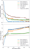 |
Fig. 2 Composition (top) and specific entropy (bottom) vs. normalised mass at the time when proto-Jupiter reached its final mass (at 2.6 × 10⁴ (Hot_compact_Z & Hot_extended_Z) and 2.6 × 10⁶ years (Cold_extended_Z & Cold_high_Z). In both figures, thicker lines depict convective regions. For comparison, we also show how the accreted heavy-element profile without mixing (grey dashed) for Hot_extended_Z, as well as composition and entropy from Vazan et al. (2018) (red dotted). The black dash-dotted line depicts roughly current Jupiter’s entropy S ≃ 6.2 kB baryon−1 (Marley et al. 2007). |
3.2 Jupiter’s evolution after formation
Inhibiting convection at early times can be significant for Jupiter today. This is because mixing is most efficient when the planet is young and hot, and convective luminosities are large. In addition to the radiative envelope created due to the accretion shock, a composition profile could further stabilise the envelope against large-scale convection. In Fig. 3, we show the location of the bottom of the largest convection zone (qbot = mbot∕MJ) as Jupiter evolves and contracts. Below this mass coordinate there could still be small convection zones, but no large-scale convection that thoroughly mixes the heavy elements into the envelope. We denote the region below the largest convection zone as the dilute core region in Fig. 3. For comparison, the dashed lines depict the boundary of the fuzzy core as presented in structure models.
Hot_compact_Z & Hot_extended_Z have similar behaviours. As Jupiter contracts and cools down, the convection zone quickly propagates inwards in ~105 yr, until it stops when it reaches the steep, primordial composition gradient (qbot ≃ 0.2). Despite the accreted heavy-element gradient in Hot_extended_Z, the convection zone advances at a similar pace. This demonstrates that the heavy-element gradient is insufficient to stop large-scale convection in the envelope. The reason is the large amount of thermal energy that is available to drive convection. Cold_extended_Z begins slightly more convective (see Fig. 2). In the first few thousand years, the convection zone retreats, because the mixing of heavy elements transiently stabilises the envelope. After that, the behaviour is very close to that of the other models, except that it takes longer (~ 106 yr) to reach the stalling point. This is because there is less thermal energy available since the accretion was slow and the surface temperaturewas not affected by the shock. Cold_high_Z behaves very similarly, except that the outer convection zone is smaller at a given time compared to the other models. Also, there can be large dredge-up events, where heavy elements from the deep envelope are mixed into the upper envelope, shutting down convection for a short time.
All our models lead to a similar outcome: after, at most, a few tens of millions of years, the envelope is mostly mixed down to qbot ≲ 0.2, and there is onlya small dilute-core region still intact. This implies that standard formation models cannot lead to an extended fuzzy core.
The propagation and stalling of the convection zone can be understood in the following way, as discussed previously in Vazan et al. (2018). The convective part of the envelope is cooling faster than the radiative/conductive region, as energy is transported to the surface by the convective flux. The boundary is characterised by an increasingly destabilising temperature gradient, and the convection zone moves inwards.
However, at higher density, thermal conduction becomes more efficient, and the system can reach a quasi-steady state in which the conductive heat transport across the boundary is sufficient to carry the full cooling luminosity. The difference intemperature between radiative and convective shells stops growing, never becoming large enough to overcome the stabilising composition in the deep interior, and the innermost part of the dilute core is stable on a Gyr timescale.
There are likely to be additional physical mechanisms not included in our calculations that act to mix heavy elements across the thin boundary layers that separate convective regions. For example, turbulent motions could at least partially penetrate the boundary and act to transport heavy elements across the interfaces (Canuto 1998, 1999; Herwig 2000; Moll et al. 2017). However, this would only further dilute the composition profile and allow the outer homogeneously mixed region to penetrate even deeper into the interior. Including additional mixing mechanisms would therefore only strengthen our conclusions about the difficulty of making an extended core.
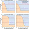 |
Fig. 3 Mass coordinate at the bottom of the largest convection zone (qbot = mbot∕M) as Jupiter evolves. We define the age to be zero at the point where Jupiter reaches its final mass and gas accretion has stopped. Curves are smoothed slightly in order to increase readability. |
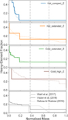 |
Fig. 4 Heavy-element mass fraction vs. normalised mass of Jupiter shortly after its formation (dashed coloured lines) and today (solid coloured lines). The different panels (and colours) show the different formation pathways we consider. The grey vertical dashed lines indicate the extent of the dilute-coreregion as inferred by recent evolution (Vazan et al. 2018) and structure models (Wahl et al. 2017; Debras & Chabrier 2019). In all of our models, the dilute-core region is substantially smaller by ≲ 50% by mass. The bottom panel shows the heavy-element distribution of these published models (solid grey lines). |
3.3 Final structure
As shown in Fig. 3, in all the cases we consider, the outer convection zone never reaches the deepest interior. This is demonstrated in Fig. 4, which shows the heavy-element distribution as a function of normalised mass of our models at Jupiter’s current age, compared to those of Wahl et al. (2017), Vazan et al. (2018), and Debras & Chabrier (2019). The extent of the dilute core can be identified as the location of the outer-most significant jump in the metal content, which in our models occurs at a mass of m ≲ 0.20 MJ, which translates roughly intor ≲ 0.40 RJ. Hot_compact_Z shows a stable configuration where the primordial composition gradient was modified by the formation of several small convection zones in the deep interior, resulting in a structure with many convective-conductive interfaces. This can be identified by the several jumps in composition. The heavy elements from the primordial gradient are barely mixed into the envelope, and the metallicity at the 1-bar level remains at Z1bar = 0.04, as set by the accretion.
While the models Hot_extended_Z and Cold_extended_Z have very different accretion histories, the final structure is similar. The envelope is homogeneously mixed down to a radius of r ≃ 0.4 RJ, where a thin convective-conductive interface separates two convection zones. Additionally, some of the heavy elements of the primordial composition are mixed into the outer envelope, increasing the metallicity of the outer envelope to Z1bar = 0.12. It should be noted that the dilute core is roughly the same size in all models, including Cold_high_Z. This is because the mass of the steep primordial composition gradient is constrained by the planet’s mass at the onset of rapid gas accretion. By comparison, in Wahl et al. (2017), Vazan et al. (2018), and Debras & Chabrier (2019), the dilute core occupies a region larger than 0.5 RJ. The inferred density profiles from our evolution models are shown in Fig. 5. The density in our models is higher than the one inferred by structure models since they are colder, consist of more heavy elements, and do not satisfy all the observational properties of Jupiter today. It should be noted that these models are not meant to fit Jupiter’s interior exactly. The goal of this study is to explore formation paths that can lead to an extended dilute core. As a result, formation with high accretion rates of heavy elements are preferred.
Our models are summarised in Table 2, where we list the radius, total heavy-element mass, calculated normalised moment of inertia (MoI), effective and 1-bar temperatures, and the heavy-element fraction at 1 bar. None of our models are within the observational uncertainties of Jupiter’s observed values. This is not surprising, since our Jupiter models are highly enriched in metals. Additionally, our model makes a number of necessary simplifications. Therefore, even if we had the right amount of heavy elements, our models would not lead to Jupiter exactly. Among other things, the heavy elements are represented by pure water, the planet is assumed to be spherical and non-rotating, and our atmospheric model is simple. In addition, we do not consider helium rain (Stevenson 1975; Fortney & Hubbard 2004; Wilson & Militzer 2010). However, the pressures and temperatures at the dilute-core boundary are far outside the H–He separation regime (Morales et al. 2009, 2013; Schöttler & Redmer 2018), and therefore helium rain is not expected to affect the characteristics of the dilute core. Helium rain is more relevant for Saturn, since H–He separation occurs in the deep interior, closer to the planetary centre.
Another mechanism that could affect the heavy-element distribution within the planet is core erosion. The details of this mechanism, however, are uncertain (Guillot et al. 2004) and depend on the material properties (Wilson & Militzer 2012; Soubiran & Militzer 2016). In the simple models of Guillot et al. (2004), core erosion is seen as the entrainment of the core material into the convection zone. A fraction of the kinetic energy in convection is used to mix heavy elements from the core into the convective envelope. If convective mixing is efficient, the material coming from the core would likely homogeneously mix into the envelope instead of forming a dilute core. It is plausible that at later stages in Jupiter’s evolution, convection is less vigorous, and the eroded core material could create a composition gradient where semi-convection operates. However, the details of this process are beyond the scope of this paper and require a detailed investigation. We hope to address this in future research.
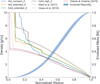 |
Fig. 5 Density vs. normalised radius for our four Jupiter models (solid), and the dilute-core models of Wahl et al. (2017) (dashed grey), Vazan et al. (2018) (dotted purple) and Debras & Chabrier (2019) (dashed red). The shaded blue region shows the range of possible enclosed masses for all density profiles. |
Summary of our models at 4.5 Gyrs and measured/inferred values for Jupiter.
3.4 Sensitivity of the results to model assumptions
In this section, we investigate the sensitivity of our results to the assumed model parameters including the EoSs, opacities, and the possibility of semi-convection. We take model Cold_extended_Z as the reference case. We show that while there are small changes in the heavy-element distribution, our conclusion that the extent of the dilute core region cannot extend beyond ~ 20% of the planetary mass is robust.
3.4.1 Equation of state
As discussed in Sect. 2, in all the models presented above, the heavy elements were represented by water. Denser materials (e.g. rocks, metals) have higher molecular weights, and therefore are harder to mix, and are more effective in suppressing convection (Vazan et al. 2015). Since the heavy elements in giant planets could include refractory materials, the models above might overestimate the efficiency of mixing. We therefore also ran models in which the heavy elements were represented by SiO2 (rock). The SiO2 EoS was again the QEoS from More et al. (1988). In addition, we created a 50/50 mixture of rock & water by combining their respective EoS, assuming ideal mixing. Since Jupiter’s composition is dominated by hydrogen and helium, we also present a model in which the H–He EoS is calculated with the SCvH (Saumon et al. 1995) table instead of the newer version of Chabrier et al. (2019) (denoted by CMS) that we have implemented for the baseline cases. Figure 6 shows the heavy-element distribution in Jupiter today when using different EoSs, as described above. While the EoS clearly has an effect on the mixing in the deep interior, the location of the dilute core is unaffected.
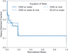 |
Fig. 6 Heavy-element mass fraction vs. normalised mass in Jupiter today. The dashed line depicts our reference model Cold_extended_Z calculated with the CMS EoS for H/He (Chabrier et al. 2019) and QEoS for water (More et al. 1988). The various solid lines are the same model calculated with different EoSs (see Sect. 3.4.1). |
3.4.2 Opacity
Another important ingredient in the evolution calculation is the assumed opacity and whether it includes the contribution from grains since this can have a strong influence on the planetary cooling. As a result, the mixing in the interior and the extent of the dilute core can also be affected. To test the robustness of our results to the assumed opacity, we re-calculated the evolution of Cold_extended_Z once with grain opacity included (see Sect. 2.1). We also separately scaled the conductive opacity by a factor η = 0.01, 0.1, 10, 100. In Fig. 7, we show the inferred heavy-element profile in Jupiter today for the different models. Although the exact distribution of the heavy elements depends on the assumed opacity, the location of the dilute core remains unchanged. The only model where the location of the dilute core shifts is when the conductive opacity is reduced by a factor of 100. This is because an increase in the conductivity stabilises the conductive/convective interface, and the energy can be transported through the interface more efficiently.
We find that an increased opacity generally leads to the stairs being less stable. However, there is no qualitative difference in the final heavy-element profile when the conductive opacity is increased or decreased by a factor of 10. As a result, even if the conductive opacity used in this work is not ideal for Jupiter’s interior, it suggests that our main conclusion rather insensitive to the assumedopacity.
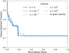 |
Fig. 7 Heavy-element fraction vs. normalised mass in Jupiter today. The dashed line depicts our reference model Cold_extended_Z calculated without the grain contribution to the opacity. The various solid lines are the same model calculated with either the conductive opacity scaled by a factor η or with grain opacity included (see Sect. 3.4.2). |
3.4.3 Semi-convection
Our baseline models were calculated without considering semi-convection in Ledoux-stable but Schwarzschild-unstable regions. Semi-convection could destabilise composition gradients by allowing for an efficient transport of heat across double-diffusive layers (see Sect. 2.1). We therefore re-calculated Cold_extended_Z when enabling semi-convection with a range of αsc, which can be interpreted as the typical layer height (measured in pressure scale heights) of the double-diffusive regions. The resulting heavy-element profile is presented in Fig. 8. We find that including semi-convection does not yield significantly different heavy-element profiles in our models. In particular, the extent of the dilute core is largely unaffected.
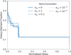 |
Fig. 8 Heavy-element fraction vs. normalised mass in Jupiter today. The dashed line depicts our reference model Cold_extended_Z calculated without semi-convection. The various solid lines are the same model calculated with semi-convection included and a specific αsc (see Sect. 3.4.3). |
4 Connection to interior models of Jupiter
Recent interior models of Jupiter suggest that the classic view of a simple core-envelope structure cannot be brought into accordance with observations (Wahl et al. 2017; Debras & Chabrier 2019). Instead, in order to satisfy the gravity data, an internal structure with a dilute core seems to be required. In fact, there is no clear definition of a “dilute or fuzzy core”. What is usually meant is that there isa region in the innermost part of the planet that is enriched in heavy elements, possibly in the form of composition gradients, that extends far into the envelope (Helled & Stevenson 2017). The dilute core presented by Wahl et al. (2017) extends to ≃0.5 RJ, and is a region that is enriched with heavy elements by a constant factor compared to the outer envelope. In the models of Debras & Chabrier (2019), the dilute core corresponds to linearly decreasing the heavy-element fraction up to ≃ 0.7 RJ, going from Z ≃ 0.2 in the deep interior to a few times solar. Nevertheless, in both models, the dilute core spans a large fraction of Jupiter’s radius (and mass).
In both Wahl et al. (2017) and Debras & Chabrier (2019), the extent of the dilute-core region was adjusted so that the resulting density profile matches Jupiter’s gravitational moments as measured by Juno (Folkner et al. 2017; Iess et al. 2018). In Wahl et al. (2017), the dilute-core boundary was modelled as a step function-like drop in the heavy-element fraction, while Debras & Chabrier (2019) used a linearly decreasing function. In these models, the authors justify the stability of this region by invoking semi-convection to this inner-most part. These two interior structure models also use a different EoSs for H–He, which leads to a different envelope metallicity. An important point is that the location of the dilute core is empirical - it is not a result of a physical process or the transport properties of the chemical elements.
Our study suggests that such an extended composition gradient is not a natural outcome of formation and evolution models. We begin with a primordial composition gradient in the deep interior that was present before Jupiter acquired its massive gaseous envelope. Asa result, the extent of the dilute core at this point is limited by proto-Jupiter’s mass at the onset of runaway gas accretion (≃ 20% of the mass in our models above). One may naively think that it should be possible to create a composition gradient that is less steep and spans more of the planet’s mass by, for example, slowly eroding the heavy-element gradient and constructing a new, stable composition gradient that is less steep. However, our calculations show that this is not the case. As Jupiter’s radiative envelope cools down and the convection zone pushes inwards, heavy elements are transported outwards, but in that case they become homogeneously mixed across the entire outer convection zone. Alternatively, thermal conduction across the boundary can stabilise the boundary, as discussed in Sect. 3.2. In this case, however, we find that the interior composition gradient forms a staircase of convective layers that maintain the overall mean composition gradient, so that the heavy elements remain in the innermost region.
Model Cold_high_Z was set to be very favourable to create a final structure with an extended dilute core. Firstly, ≃ 60 M⊕ of heavy elements were accreted during runaway gas accretion to form a massive composition gradient that spans the entire envelope by construction. Secondly, the accretion parameters were chosen to yield a “cold” Jupiter to reduce the convective luminosity available for mixing. However, even in this model, the outer regions quickly destabilise, since the stabilising effect of the composition is insufficient to stop the outer convection zone from advancing inwards. Only the deep interior, where the composition gradient is very steep, remains unmixed.
In Vazan et al. (2018), the composition gradient remains mostly intact throughout Jupiter’s lifetime, and only the outer envelope becomes fully mixed. The difference between our results and the calculation of Vazan et al. (2018) can be explained by the way in which the models are constructed. In Vazan et al. (2018), the initial temperature and composition profile were chosen ad-hoc such that the final structure at 4.5 Gyrs matches observations. The formation process was not modelled, rather the evolution calculation began with a fully formed Jupiter. As a result, their initial model is significantly colder than ours (see Fig. 2), and therefore, mixing is less efficient. In this study, we followed Jupiter’s formation and modelled the runaway phase, which leads to higher entropy (and therefore hotter) envelopes. Even in our attempt to make the coldest possible models, the entropy is still significantly higher than in Vazan et al. (2018).
We therefore conclude that it is extremely challenging for standard formation models to arrive at a dilute core solution as inferred from structure models that fit Juno’s gravity measurements. There are a few reasons for that. Firstly, the stable composition gradient is constrained to the deep interior because it is already present at the onset of runaway gas accretion. Secondly, if the dilute core is a result of the runaway gas accretion, then it is not stable against convection unless proto-Jupiter is unrealistically cold, which seems rather unlikely (Berardo & Cumming 2017; Cumming et al. 2018). It also requires extremely large amounts of heavy elements to be accreted, which is not possible if Jupiter formed in-situ (Shibata et al. 2020). Thus, in order to reach a dilute core in Jupiter, additional mechanisms are required. One possibility is a vast migration of Jupiter. Indeed, recent numerical simulations of planetesimal accretion that include Jupiter’s migration suggest that it could capture tens of M⊕ of heavy elements (Shibata et al. 2020), if the protoplanetary disc is sufficiently massive. This would mean that Jupiter must have migrated over a large distance, for example starting at ~ 10 au. It should be noted, however, that this does not guarantee that the envelope would be stable against large scale convection, as demonstrated in case Cold_high_Z.
Another potential path to form a dilute core is via a giant impact, as suggested by Liu et al. (2019). In this scenario, a giant impactor (~10 M⊕) provides theenergy necessary to disrupt the primordial compact core and mix the heavy elements into the envelope. Liu et al. (2019) showed that under certain conditions (impact parameters and initial thermal state of Jupiter), the extended dilute core is stable over Jupiter’s lifetime. In fact, our models suggest that such a giant impact must occur at a relatively later stage when Jupiter is cold enough to avoid significant mixing of the interior.
Our results suggest standard formation paths are unlikely to create an extended dilute-core structure unless additional physical processes such as layered convection (Leconte & Chabrier 2012) or core erosion (Guillot et al. 2004; Moll et al. 2017), a giant impact, or significant migration are included. Even for these scenarios, a detailed investigation is still needed, and a process that leads to the formation of Jupiter’s dilute core is yet to be presented.
5 Summary
We calculated the formation and long-term evolution of Jupiter starting from the onset of runaway gas accretion until today, properly accounting for the energy transport and heavy-element mixing in the deep interior. We investigated different formation scenarios, with primordial composition gradients and various heavy-element accretion rates and shock properties during runaway gas accretion. Our main findings can be summarised as follows:
-
If Jupiter accretes a homogeneous envelope on top of a primordial composition gradient of heavy-elements (model Hot_compact_Z), mixing in the deep interior leaves the original structure mostly intact. Almost none of the heavy elementsare mixed into the envelope – the dilute core is too compact.
-
If the composition gradient is the result of a large amount of heavy-element accretion during runaway, the envelope quickly (~106 yr) becomes unstable in the face of large-scale convection (models Hot_extended_Z & Cold_extended_Z). The result is a fully mixed envelope, with a small dilute core in the deep interior.
-
Even a cold and slow runaway gas accretion (τacc ~ 106 yr) combined with a very high accreted mass of solids (≃60 M⊕) leads to a formation path where the outer convection zone destroys the accreted composition gradient (model Cold_high_Z).
-
None of our models lead to a structure of Jupiter today with an extended dilute core. Current interior models require a dilute core that has an extent of ≃0.5–0.7 RJ, significantly larger than found in this study.
We conclude that forming a fuzzy core in Jupiter as suggested by recent studies is in fact very challenging in the standard picture of giant planet formation. One solution for Jupiter’s extended dilute core is a giant impact. However, this must have occurred late, otherwise Jupiter would have been too hot, and convection would have been too efficient for the composition gradient to survive. Future works should focus on the correct modelling of additional processes that could influence the mixing, such as helium rain, double-diffusive convection, and core erosion, as well as the development of more sophisticated formation models.
Acknowledgements
We thank S. Mazevet for the careful reading of the paper and valuable comments. We also thank D. Stevenson, P. Bodenheimer and A. Vazan for fruitful discussions, and F. Debras and G. Chabrier for sharing their data with us. We also acknowledge support from SNSF grant 200020_188460 and the National Centre for Competence in Research “PlanetS” supported by SNSF. AC is supported by an NSERC Discovery grant and is a member of the Centre de Recherche en Astrophysique du Québec (CRAQ) and the Institut de recherche sur les exoplanètes (iREx).
Appendix A Equation of state
For the temperature/density regime relevant for planetary modelling, MESA includes the SCvH (Saumon et al. 1995) EoS tables for mixturesof hydrogen and helium. In this regime, however, the tables do not include the contribution from heavy elements. A common approach to bypass this issue is to model the planet as consisting of an inert core that is treated as an inner boundary condition for the structure equations, and a gaseous hydrogen-helium envelope (see, e.g. Malsky & Rogers 2020). However, this approach does not work if one wants to follow the mixing of heavy elements, for example. Therefore, we implemented an EoS into MESA that is suitable for planetary interior conditions and includes either water or rock as a heavy element. Our EoS is an updated version of the EoS from Vazan et al. (2013), where the two equations of state SCvH (Saumon et al. 1995) for hydrogen and helium and QEoS (More et al. 1988) for water or rock (SiO2) were combined to allow for an arbitrary mixture of the three components, by replacing the SCvH with the recent H–He EoS of Chabrier et al. (2019).
The calculation of mixtures makes use of the additive volume law 1∕ρ(p, T, X) = X∕ρH(p, T) + Y∕ρHe(p, T) + Z∕ρZ(p, T), where we denote the dependence on an arbitrary composition by X andX, Y, Z are the mass fractions of hydrogen, helium, and the heavy elements, respectively. The required thermodynamic quantities such as the entropy follow similar additive laws. We neglect the entropy of mixing, as it is a small correction that does not have a significant impact on planetary evolution (Baraffe et al. 2008).
To implement this EoS into MESA, we created a grid of tables with compositions varying by ΔX, ΔZ = 0.1 in the range of 0 ≤ Z ≤ 1 and 0 ≤ X ≤ 1. The tables were calculated on a grid of log Q and log T, where log Q = log ρ − 2log T + 12. These tables are then read and used for the evolution calculations by the EoS module in MESA, with a few modifications. The module then calculates the required thermodynamic quantities for a mixture of hydrogen, helium, and the heavy elements by interpolating between the tables. Water (and rock) undergoes phase transitions at certain relevant pressures and temperatures. This introduces discontinuities in the derivatives of thermodynamic variables. Since every entry in the tables needs to be valid, we smoothed over phase transitions with a cubic spline interpolation that uses the closest valid neighbouring points.
In Fig. A.1, we show the cooling of two homogeneously mixed one Jupiter-mass planets calculated with MESA using our equation of state. The difference between the two models is only the bulk metallicity, which is Z = 0.02, 0.50, respectively. As expected, the metal-rich planet is much denser and hotter than the metal-poor one. Both cooling tracks are well within the equation of state boundaries (dashed black lines), demonstrating that the current range is sufficient.
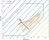 |
Fig. A.1 Cooling of two homogeneous one Jupiter mass planets in the log ρ- log T plane calculated with our version of MESA that includes the modified equation of state. One of them is metal-poor (orange), and the other is metal-rich (dashed grey). The contours correspond to values of log Q = log ρ − 2log T + 12. Dashed black lines show the boundaries beyond which the equation of state is not valid. The arrow indicates the direction of time. |
As an additional test to see whether our EoS is working properly, we reproduced the results from Vazan et al. (2018) by calculating Jupiter’s evolution starting with the same temperature and composition profiles. While there were some small differences in the final interior structure at Jupiter’s age (due to different opacities, resolutions, and numerical methods), we got a very similar result, in particular regarding the extent of the dilute core. We therefore conclude that our EoS implementation in MESA is working reliably.
A limitation of our EoS implementation is that we do not currently include the effect of heavy elements in the compressional heating term ɛg in the energy equation (see discussion in Sect. 2.5 of Mankovich et al. 2016). We find that there are numerical difficulties, because the extra derivative would have to be calculated by a simple two point estimation, which is numerically noisy and leads to unreliable results. We leave this for future works.
References
- Baraffe, I., Chabrier, G., & Barman, T. 2008, A&A, 482, 315 [NASA ADS] [CrossRef] [EDP Sciences] [Google Scholar]
- Berardo, D., & Cumming, A. 2017, ApJ, 846, L17 [NASA ADS] [CrossRef] [Google Scholar]
- Berardo, D., Cumming, A., & Marleau, G.-D. 2017, ApJ, 834, 149 [NASA ADS] [CrossRef] [Google Scholar]
- Bolton, S. J., Lunine, J., Stevenson, D., et al. 2017, Space Sci. Rev., 213, 5 [NASA ADS] [CrossRef] [Google Scholar]
- Canuto, V. M. 1998, ApJ, 508, 767 [NASA ADS] [CrossRef] [Google Scholar]
- Canuto, V. M. 1999, ApJ, 524, 311 [NASA ADS] [CrossRef] [Google Scholar]
- Cassisi, S., Potekhin, A. Y., Pietrinferni, A., Catelan, M., & Salaris, M. 2007, ApJ, 661, 1094 [NASA ADS] [CrossRef] [Google Scholar]
- Chabrier, G., & Baraffe, I. 2007, ApJ, 661, L81 [Google Scholar]
- Chabrier, G., Mazevet, S., & Soubiran, F. 2019, ApJ, 872, 51 [NASA ADS] [CrossRef] [Google Scholar]
- Cumming, A., Helled, R., & Venturini, J. 2018, MNRAS, 477, 4817 [Google Scholar]
- Debras, F., & Chabrier, G. 2019, ApJ, 872, 100 [NASA ADS] [CrossRef] [Google Scholar]
- Ferguson, J. W., Alexander, D. R., Allard, F., et al. 2005, ApJ, 623, 585 [NASA ADS] [CrossRef] [Google Scholar]
- Folkner, W. M., Iess, L., Anderson, J. D., et al. 2017, Geophys. Res. Lett., 44, 4694 [NASA ADS] [CrossRef] [Google Scholar]
- Fortney, J. J., & Hubbard, W. B. 2004, ApJ, 608, 1039 [NASA ADS] [CrossRef] [Google Scholar]
- Freedman, R. S., Marley, M. S., & Lodders, K. 2008, ApJS, 174, 504 [NASA ADS] [CrossRef] [Google Scholar]
- French, M., Mattsson, T. R., Nettelmann, N., & Redmer, R. 2009, Phys. Rev. B, 79, 054107 [NASA ADS] [CrossRef] [Google Scholar]
- Guillot, T. 2005, Ann. Rev. Earth Planet. Sci., 33, 493 [NASA ADS] [CrossRef] [MathSciNet] [PubMed] [Google Scholar]
- Guillot, T., Stevenson, D. J., Hubbard, W. B., & Saumon, D. 2004, The Interior of Jupiter, ed. F. Bagenal, T. E. Dowling, & W. B. McKinnon (Washington: Nasa), 1, 35 [Google Scholar]
- Helled, R., & Stevenson, D. 2017, ApJ, 840, L4 [NASA ADS] [CrossRef] [Google Scholar]
- Henyey, L., Vardya, M. S., & Bodenheimer, P. 1965, ApJ, 142, 841 [NASA ADS] [CrossRef] [Google Scholar]
- Herwig, F. 2000, A&A, 360, 952 [NASA ADS] [Google Scholar]
- Iess, L., Folkner, W. M., Durante, D., et al. 2018, Nature, 555, 220 [NASA ADS] [CrossRef] [Google Scholar]
- Kippenhahn, R., Weigert, A., & Weiss, A. 2012, Stellar Structure and Evolution (Berlin: Springer) [Google Scholar]
- Langer, N., Fricke, K. J., & Sugimoto, D. 1983, A&A, 126, 207 [NASA ADS] [Google Scholar]
- Langer, N., El Eid, M. F., & Fricke, K. J. 1985, A&A, 145, 179 [NASA ADS] [Google Scholar]
- Leconte, J., & Chabrier, G. 2012, A&A, 540, A20 [NASA ADS] [CrossRef] [EDP Sciences] [Google Scholar]
- Lissauer, J. J., Hubickyj, O., D’Angelo, G., & Bodenheimer, P. 2009, Icarus, 199, 338 [NASA ADS] [CrossRef] [Google Scholar]
- Liu, S.-F., Hori, Y., Müller, S., et al. 2019, Nature, 572, 355 [CrossRef] [Google Scholar]
- Lozovsky, M., Helled, R., Rosenberg, E. D., & Bodenheimer, P. 2017, ApJ, 836, 227 [NASA ADS] [CrossRef] [Google Scholar]
- Malsky, I., & Rogers, L. A. 2020, ApJ, 896, 48 [Google Scholar]
- Mankovich, C., Fortney, J. J., & Moore, K. L. 2016, ApJ, 832, 113 [NASA ADS] [CrossRef] [Google Scholar]
- Marleau, G.-D., Klahr, H., Kuiper, R., & Mordasini, C. 2017, ApJ, 836, 221 [Google Scholar]
- Marleau, G.-D., Mordasini, C., & Kuiper, R. 2019, ApJ, 881, 144 [NASA ADS] [CrossRef] [EDP Sciences] [Google Scholar]
- Marley, M. S., Fortney, J. J., Hubickyj, O., Bodenheimer, P., & Lissauer, J. J. 2007, ApJ, 655, 541 [NASA ADS] [CrossRef] [Google Scholar]
- Mazevet, S., Musella, R., & Guyot, F. 2019a, A&A, 631, L4 [NASA ADS] [CrossRef] [EDP Sciences] [Google Scholar]
- Mazevet,S., Licari, A., Chabrier, G., & Potekhin, A. Y. 2019b, A&A, 621, A128 [NASA ADS] [CrossRef] [EDP Sciences] [Google Scholar]
- Mizuno, H. 1980, Prog. Theor. Phys., 64, 544 [Google Scholar]
- Moll, R., Garaud, P., Mankovich, C., & Fortney, J. J. 2017, ApJ, 849, 24 [Google Scholar]
- Morales, M. A., Schwegler, E., Ceperley, D., et al. 2009, Proc. Natl Acad. Sci., 106, 1324 [Google Scholar]
- Morales, M. A., Hamel, S., Caspersen, K., & Schwegler, E. 2013, Phys. Rev. B, 87, 174105 [NASA ADS] [CrossRef] [Google Scholar]
- More, R. M., Warren, K. H., Young, D. A., & Zimmerman, G. B. 1988, Phys. Fluids, 31, 3059 [NASA ADS] [CrossRef] [Google Scholar]
- Paxton, B., Bildsten, L., Dotter, A., et al. 2011, ApJS, 192, 3 [Google Scholar]
- Paxton, B., Cantiello, M., Arras, P., et al. 2013, ApJS, 208, 4 [NASA ADS] [CrossRef] [Google Scholar]
- Paxton, B., Marchant, P., Schwab, J., et al. 2015, ApJS, 220, 15 [Google Scholar]
- Paxton, B., Schwab, J., Bauer, E. B., et al. 2018, ApJS, 234, 34 [NASA ADS] [CrossRef] [EDP Sciences] [Google Scholar]
- Paxton, B., Smolec, R., Schwab, J., et al. 2019, ApJS, 243, 10 [NASA ADS] [CrossRef] [PubMed] [Google Scholar]
- Podolak, M., Helled, R., & Schubert, G. 2019, MNRAS, 487, 2653 [NASA ADS] [CrossRef] [Google Scholar]
- Pollack, J. B., Hubickyj, O., Bodenheimer, P., et al. 1996, Icarus, 124, 62 [NASA ADS] [CrossRef] [Google Scholar]
- Radko, T., Bulters, A., Flanagan, J. D., & Campin, J. M. 2014, J. Phys. Oceanogr., 44, 1269 [NASA ADS] [CrossRef] [Google Scholar]
- Saumon, D., Chabrier, G., & van Horn, H. M. 1995, ApJS, 99, 713 [NASA ADS] [CrossRef] [Google Scholar]
- Schöttler, M., & Redmer, R. 2018, Phys. Rev. Lett., 120, 115703 [NASA ADS] [CrossRef] [Google Scholar]
- Shibata, S., Helled, R., & Ikoma, M. 2020, A&A, 633, A33 [Google Scholar]
- Soubiran, F., & Militzer, B. 2016, ApJ, 829, 14 [CrossRef] [Google Scholar]
- Soubiran, F., Militzer, B., Driver, K. P., & Zhang, S. 2017, Phys. Plasmas, 24, 041401 [NASA ADS] [CrossRef] [Google Scholar]
- Stevenson, D. J. 1975, Phys. Rev. B, 12, 3999 [NASA ADS] [CrossRef] [Google Scholar]
- Stevenson, D. J. 1982, Ann. Rev. Earth Planet. Sci., 10, 257 [NASA ADS] [CrossRef] [Google Scholar]
- Stevenson, D. J. 1985, Icarus, 62, 4 [NASA ADS] [CrossRef] [Google Scholar]
- Valencia, D., Guillot, T., Parmentier, V., & Freedman, R. S. 2013, ApJ, 775, 10 [NASA ADS] [CrossRef] [Google Scholar]
- Vazan, A., Kovetz, A., Podolak, M., & Helled, R. 2013, MNRAS, 434, 3283 [NASA ADS] [CrossRef] [Google Scholar]
- Vazan, A., Helled, R., Kovetz, A., & Podolak, M. 2015, ApJ, 803, 32 [NASA ADS] [CrossRef] [Google Scholar]
- Vazan, A., Helled, R., Podolak, M., & Kovetz, A. 2016, ApJ, 829, 118 [Google Scholar]
- Vazan, A., Helled, R., & Guillot, T. 2018, A&A, 610, L14 [Google Scholar]
- Wahl, S. M., Hubbard, W. B., Militzer, B., et al. 2017, Geophys. Res. Lett., 44, 4649 [NASA ADS] [CrossRef] [Google Scholar]
- Wilson, H. F., & Militzer, B. 2010, Phys. Rev. Lett., 104, 121101 [Google Scholar]
- Wilson, H. F., & Militzer, B. 2012, ApJ, 745, 54 [NASA ADS] [CrossRef] [Google Scholar]
- Wood, T. S., Garaud, P., & Stellmach, S. 2013, ApJ, 768, 157 [NASA ADS] [CrossRef] [Google Scholar]
All Tables
Summary of our models at the onset of the runaway accretion phase (Mtot = 58 M⊕) and the accretion parameters.
All Figures
|
Fig. 1 Heavy-element distribution in proto-Jupiter vs. mass at the onset of runaway gas accretion for the different models. The total mass in each model is M = 58 M⊕, and the totalheavy element masses are MZ = 23 (Hot_compact_Z) 16 (Hot/Cold_extended_Z) and 28 M⊕ (Cold_extended_Z). |
| In the text | |
|
Fig. 2 Composition (top) and specific entropy (bottom) vs. normalised mass at the time when proto-Jupiter reached its final mass (at 2.6 × 10⁴ (Hot_compact_Z & Hot_extended_Z) and 2.6 × 10⁶ years (Cold_extended_Z & Cold_high_Z). In both figures, thicker lines depict convective regions. For comparison, we also show how the accreted heavy-element profile without mixing (grey dashed) for Hot_extended_Z, as well as composition and entropy from Vazan et al. (2018) (red dotted). The black dash-dotted line depicts roughly current Jupiter’s entropy S ≃ 6.2 kB baryon−1 (Marley et al. 2007). |
| In the text | |
|
Fig. 3 Mass coordinate at the bottom of the largest convection zone (qbot = mbot∕M) as Jupiter evolves. We define the age to be zero at the point where Jupiter reaches its final mass and gas accretion has stopped. Curves are smoothed slightly in order to increase readability. |
| In the text | |
|
Fig. 4 Heavy-element mass fraction vs. normalised mass of Jupiter shortly after its formation (dashed coloured lines) and today (solid coloured lines). The different panels (and colours) show the different formation pathways we consider. The grey vertical dashed lines indicate the extent of the dilute-coreregion as inferred by recent evolution (Vazan et al. 2018) and structure models (Wahl et al. 2017; Debras & Chabrier 2019). In all of our models, the dilute-core region is substantially smaller by ≲ 50% by mass. The bottom panel shows the heavy-element distribution of these published models (solid grey lines). |
| In the text | |
|
Fig. 5 Density vs. normalised radius for our four Jupiter models (solid), and the dilute-core models of Wahl et al. (2017) (dashed grey), Vazan et al. (2018) (dotted purple) and Debras & Chabrier (2019) (dashed red). The shaded blue region shows the range of possible enclosed masses for all density profiles. |
| In the text | |
|
Fig. 6 Heavy-element mass fraction vs. normalised mass in Jupiter today. The dashed line depicts our reference model Cold_extended_Z calculated with the CMS EoS for H/He (Chabrier et al. 2019) and QEoS for water (More et al. 1988). The various solid lines are the same model calculated with different EoSs (see Sect. 3.4.1). |
| In the text | |
|
Fig. 7 Heavy-element fraction vs. normalised mass in Jupiter today. The dashed line depicts our reference model Cold_extended_Z calculated without the grain contribution to the opacity. The various solid lines are the same model calculated with either the conductive opacity scaled by a factor η or with grain opacity included (see Sect. 3.4.2). |
| In the text | |
|
Fig. 8 Heavy-element fraction vs. normalised mass in Jupiter today. The dashed line depicts our reference model Cold_extended_Z calculated without semi-convection. The various solid lines are the same model calculated with semi-convection included and a specific αsc (see Sect. 3.4.3). |
| In the text | |
|
Fig. A.1 Cooling of two homogeneous one Jupiter mass planets in the log ρ- log T plane calculated with our version of MESA that includes the modified equation of state. One of them is metal-poor (orange), and the other is metal-rich (dashed grey). The contours correspond to values of log Q = log ρ − 2log T + 12. Dashed black lines show the boundaries beyond which the equation of state is not valid. The arrow indicates the direction of time. |
| In the text | |
Current usage metrics show cumulative count of Article Views (full-text article views including HTML views, PDF and ePub downloads, according to the available data) and Abstracts Views on Vision4Press platform.
Data correspond to usage on the plateform after 2015. The current usage metrics is available 48-96 hours after online publication and is updated daily on week days.
Initial download of the metrics may take a while.