


| Issue |
A&A
Volume 712, August 2026
|
|
|---|---|---|
| Article Number | A35 | |
| Number of page(s) | 14 | |
| Section | Extragalactic astronomy | |
| DOI | https://doi.org/10.1051/0004-6361/202557301 | |
| Published online | 31 July 2026 | |
Investigating central star formation in local AGN host galaxies: Is there tension between coeval growth and AGN feedback?
1
Max-Planck-Institut für extraterrestrische Physik (MPE), Gießenbachstraße 1, D-85748 Garching bei München, Germany
2
Univ. Grenoble Alpes, CNRS, Grenoble INP, LPSC-IN2P3, 53, Avenue des Martyrs, 38000 Grenoble, France
3
Leibniz-Institut für Astrophysik Potsdam (AIP), An der Sternwarte 16, 14482 Potsdam, Germany
4
Max-Planck-Institut für Astrophysik (MPA), Karl-Schwarzschild-Str. 1, D-85741 Garching, Germany
★ Corresponding author: This email address is being protected from spambots. You need JavaScript enabled to view it.
Received:
18
September
2025
Accepted:
22
April
2026
Abstract
It has been argued that supermassive black holes (BHs) coevolve with the central parts of galaxies as a result of the common fuel for both the BH and star formation in the galaxy central region, as supported by the particularly significant relation between BH growth and the central mass density within 1 kpc (Σ1) found among star-forming galaxies. In the context of this scenario, one would naturally expect a close observational link between active galactic nucleus (AGN) activity and star formation activity in the central regions, e.g., the surface star formation rate density in the central 1 kpc region (ΣSFR, 1 kpc), as a manifestation of coeval growth. With ≈ 3000 galaxies in the Mapping Nearby Galaxies at Apache Point Observatory (MaNGA) survey that have X-ray coverage from SRG/eROSITA, XMM-Newton, or Chandra, we studied how the X-ray AGN fraction varies with ΣSFR, 1 kpc. We found that the fraction of X-ray AGNs with relatively higher specific BH accretion rates increases with ΣSFR, 1 kpc, consistent with the expectation. A comparison of the mean star formation rate surface density (ΣSFR) profiles of the host galaxies of these AGNs and normal galaxies sharing similar properties reveals elevated ΣSFR in AGN hosts across the entire central region. As for optically selected AGNs, their hosts also tend to show high ΣSFR in the central regions on average compared to normal galaxies, but they differ from X-ray AGNs in terms of the trend of AGN fraction versus ΣSFR, 1 kpc, which can be explained by selection effects. While these general trends all support the coeval growth scenario, they do not contradict observational evidence for AGN feedback suppressing star formation, as the average effects of such feedback might be modest in the local Universe.
Key words: galaxies: active / galaxies: evolution / galaxies: nuclei / galaxies: star formation
© The Authors 2026
 Open Access article, published by EDP Sciences, under the terms of the Creative Commons Attribution License (https://creativecommons.org/licenses/by/4.0), which permits unrestricted use, distribution, and reproduction in any medium, provided the original work is properly cited.
This article is published in open access under the Subscribe to Open model.
Open access funding provided by Max Planck Society.
1. Introduction
Supermassive black holes (BHs) are thought to coevolve with their host galaxies, as motivated by the well-established correlation between BH mass and bulge properties in the local Universe (e.g. Kormendy & Ho 2013). Two processes are generally invoked in this scenario. First, because BHs and galaxies share the same gas reservoir, some level of coeval growth is naturally expected. Second, active galactic nucleus (AGN) feedback is considered to play an important role in the regulation of galaxy evolution (e.g. Croton et al. 2006) by directly interacting with the gas reservoir via different modes and channels (e.g. Fabian 2012; Alexander & Hickox 2012; Harrison 2017).
It has been found that BH growth is closely related to various host-galaxy properties, and compactness in the galaxy central regions is particularly effective in tracking the long-term average BH growth level among star-forming (SF) galaxies (Ni et al. 2019, 2021), which supports the picture of gas in the central kiloparsec of galaxies as a common fuel for both AGNs and galaxies. In this scenario, one would expect a higher AGN fraction and/or BH growth level among galaxies with high central star formation rate (SFR), similar to what is observed for the global SFR (e.g. Chen et al. 2013; Andonie et al. 2024). At the same time, there have been some studies showing AGNs with suppressed gas fraction or star formation in the centers (e.g. Bing et al. 2019; Ellison et al. 2021; Lammers et al. 2023), which have been utilized as evidence for AGN feedback, but are potentially in tension with the picture of coeval growth.
Integral field unit (IFU) surveys are widely utilized in studies of this kind to spatially resolve the properties of AGN hosts and compare them with those of normal galaxies (that are selected to constitute a control sample). Currently, because of the limited number of James Webb Space Telescope (JWST) IFU observations and our limited understanding of how to recover a complete and unbiased sample from these available observations, this type of study has been restricted to the low-redshift Universe with IFU data from the Calar Alto Legacy Integral Field Area (CALIFA) survey (Sánchez et al. 2012), the Sydney Australian Astronomical Observatory Multi-object Integral-field Spectrograph (SAMI) Galaxy Survey (Bryant et al. 2015), and the Mapping Nearby Galaxies at Apache Point Observatory (MaNGA) survey from Sloan Digital Sky Survey IV (SDSS-IV; Bundy et al. 2015), which has the largest sample size, ideal for population studies. In different studies, AGNs are selected at different wavelengths via diverse selection criteria, and normal galaxies in the control sample are also selected differently, which might explain the wide range of (and sometimes contradictory) results arising. When comparing optically selected AGNs with normal galaxies, both suppressed central SFRs (e.g. Bing et al. 2019; Lammers et al. 2023) and elevated central SFRs (e.g. Sánchez et al. 2018; Gatto et al. 2025) are reported. Mulcahey et al. (2022) studied radio-detected AGNs (which are selected combining radio, optical, and mid-infrared diagnostics), and found that the average stellar population age (which can track specific SFR) profile of AGN hosts is similar to that of control galaxies. In addition to IFU-based studies, there have also been attempts established based on multi-band pixel-by-pixel spectral energy distribution (SED) fitting. Utilizing narrowband photometric surveys, Acharya et al. (2024) reported a suppression of specific SFR in the central regions of X-ray-selected AGN hosts compared with matched SF galaxies. While AGN selection methods vary in their respective merits and drawbacks, X-ray selection is considered to be rather clean and unbiased (e.g. Hickox & Alexander 2018). However, due to the lack of X-ray coverage with IFU surveys, previous studies based on IFU data do not fully make use of X-ray-selected AGNs in the sample.
In this work, we combined X-ray AGN selection with optical AGN selection of MaNGA galaxies to further study how AGN activity links with the star formation properties in the central regions of galaxies. We particularly aimed to resolve the potential tension between coeval growth expected from a common fuel for both the BH and the galaxy—where AGN activity is linked with elevated central star formation—and the so-called AGN negative feedback—where AGN activity is linked to suppressed central star formation. We also discuss how the AGN selection method might affect the observed results.
The paper is structured as follows. In Sect. 2 we describe the sample construction process. In Sect. 3 we detail the analysis results, and we discuss what they imply in Sect. 4. The conclusions are presented in Sect. 5. Throughout this paper, stellar masses (M★) are given in units of M⊙; SFRs are given in units of M⊙ yr−1. The surface mass density (Σ★) and that in the central 1 kpc region (Σ1) are given in units of M⊙ kpc−2; the surface density of SFR (ΣSFR) and that in the central 1 kpc region (ΣSFR, 1 kpc) are given in units of M⊙ yr−1 kpc−2. LX represents the rest-frame 2–10 keV X-ray luminosity in units of erg s−1. L[OIII] represents the (extinction-corrected) luminosity of the [O III] λ5007 emission line in units of erg s−1. LX/M★ and L[OIII]/M★ correspond to the X-ray and [O III] luminosity per unit stellar mass, respectively, in units of erg s−1 M⊙−1. Reported uncertainties are at the 1σ (68%) confidence level. A cosmology with H0 = 70 km s−1 Mpc−1, ΩM = 0.3, and ΩΛ = 0.7 is assumed.
2. Sample selection and construction
2.1. The galaxy sample obtained from MaNGA
The IFU observations from MaNGA map ≳ 10 000 nearby galaxies at z = 0.01–0.15 with 0.5 arcsec × 0.5 arcsec spaxels (Bundy et al. 2015). It covers galaxies with a relatively flat distribution in terms of i-band absolute magnitude and provides spectroscopic coverage out to 1.5 and 2.5 effective radii (re) for the primary and secondary samples, respectively. There is also a color-enhanced sample to have more objects in the low-density regions of the color-magnitude space. We started from the Sánchez et al. (2022) MaNGA pyPipe3D value-added catalog, which is built upon reduced data with version 3.1.1 of the MaNGA Data Reduction Pipeline (DRP; Law et al. 2016). All the galaxies in the main sample can be identified with the MANGA_TARGET1 flag, and there are weights provided by the DRP catalog to correct the combination of these samples to a volume-limited sample. We marked broad-line AGNs from the Oh et al. (2015) and Fu et al. (2023) catalogs, which were removed from the sample utilized in this study1. We also required objects to have z < 0.1, so that each spaxel spans over ≲ 1 kpc, which is the minimum scale we are trying to resolve in this study.
2.2. MaNGA galaxies with X-ray coverage and the selection of X-ray AGNs
2.2.1. eROSITA
We checked the MaNGA objects observed by the extended ROentgen survey with an Imaging Telescope Array (eROSITA) on board the Spektrum-Roentgen-Gamma (SRG) orbital observatory (Predehl et al. 2021), and there are 1870 objects within the coverage. As MaNGA galaxies are bright foreground galaxies with a field of view of the MaNGA fiber array ranging from 12 to 32″in diameter, we adopted a 30″matching radius (comparable to the point spread function size of eROSITA), directly matched these galaxies with the eROSITA all-sky survey data catalog from the cumulative four scans (eRASS:4), and retained matches within 3σ position errors. Then we adopted the 0.2–2.3 keV flux ML_FLUX reported in the source catalog, and converted it to LX assuming galactic absorption with Γ = 1.7. For undetected sources, we obtained the background level from the background maps and derived the minimum number of counts required for a source to be detected in the 0.2–2.3 keV band. We then derived the corresponding flux sensitivity with the corresponding energy conversion factor (ECF) = 1.074 × 10⁻¹² (e.g. Tubín-Arenas et al. 2024). We then converted this flux sensitivity at the galaxy position to LX, limit of the galaxy.
2.2.2. XMM-Newton
With the RapidXMM database (Ruiz et al. 2022), we found 890 MaNGA galaxies within XMM-Newton coverage. We also directly matched those MaNGA galaxies with the 4XMM-DR14 catalog (Webb et al. 2020) with a 30” matching radius, and adopted sources within the 3σ position error. We converted the X-ray fluxes to LX assuming a power-law model with Galactic absorption and Γ = 1.7 following the preference order of 4.5–12 keV band, and 0.2–12 keV band, thus minimizing the effects of X-ray obscuration. We also estimated LX, limit for the X-ray source to be detected at each MaNGA galaxy position, utilizing the 0.2–12 keV band flux reported in RapidXMM. A power-law model with Galactic absorption and Γ = 1.7 was again assumed through the conversion process.
2.2.3. Chandra
We made use of the Chandra Source Catalog (CSC) version 2.0 limiting sensitivity properties (Evans et al. 2024), and found 514 galaxies within Chandra coverage. The CSC provides 0.5–7 keV band flux sensitivity for a point source to be detected at a given position, and we converted this limiting flux to LX, limit via the approach reported in 2.2.2. For sources detected within the 3σChandra position error, we adopted the order of 2–7 keV band, 0.5–7 keV band, and 0.5–2 keV band to estimate LX, with assumptions similar to those above.
2.2.4. X-ray AGN selection
There are 2770 MaNGA galaxies with X-ray coverage from eROSITA, XMM-Newton, or Chandra. For each galaxy, we estimated the contribution in LX from the X-ray binary (XRB), LXRB, through a redshift-dependent function of M★ and SFR (model 269, Fragos et al. 2013), which was derived utilizing observations in Lehmer et al. (2016). We also estimated the contribution from X-ray hot gas (Mineo et al. 2012), Lgas. If LX > 3 × (LXRB + Lgas) (which is an empirical selection method for identifying sufficiently excessive X-ray emission from AGNs; see e.g., Birchall et al. 2022 for details), we classified the object as an X-ray AGN. We further classified sources with log LX < 41 as non-AGNs even if they meet this criterion, in order to remove any potential contamination from ultraluminous X-ray sources. We note that, among 10 < log M★ < 10.5 galaxies, the detected X-ray sources have luminosities comparable to the expectation from XRB contributions. Thus, we did not select X-ray AGNs with log M★ < 10.5. For log M★ > 10.5 galaxies, we can safely probe X-ray AGNs with log LX/M★ ≳ 30.5. For log M★ > 11 galaxies, X-ray AGNs can be probed down to log LX/M★ ∼ 30.
We also removed extended X-ray sources in the catalog to avoid any contamination from halo gas. For sources detected in eROSITA, we adopted the cut of the EXT_LIKE > 3; for XMM-Newton-detected sources, we adopted the cut of SC_EXT_ML > 6; for Chandra-detected sources, we used extent_flag reported in CSC. Around 20% of the X-ray sources are marked as extended.
2.3. Optical AGN selection
Among all the MaNGA galaxies with X-ray coverage, we selected optical AGNs based on the Baldwin-Phillips-Terlevich (BPT) classification diagrams in Kewley et al. (2006), where different emission line strengths are used to identify the dominant ionization mechanism, as well as the WHAN diagram (Cid Fernandes et al. 2011), where the equivalent width (EW) of Hα is utilized to remove fake AGNs (post-asymptotic giant branch stars can produce ionized gas with line ratios similar to those of low-ionization nuclear emission-line regions).
To perform the classification, we computed the flux ratios of [O III]/Hβ, [N II]/Hα, and [S II]/Hα, for valid spaxels—which are spaxels that have all these emission lines detected at S/N > 3. We then classified these valid spaxels into classes: AGN, SF, and ambiguous (Amb.). We classified a spaxel as an AGN spaxel if it was identified as an AGN in both [N II]-based and [S II]-based BPT diagrams, and has EW(Hα) > 3 Å. We classified a spaxel as SF if it was classified as SF in both BPT diagrams. Spaxels that could not be strictly classified into one of these categories were classified as ambiguous. In Fig. 1, an example of this spaxel-by-spaxel classification is presented. A general classification was then obtained by analyzing spaxels within apertures of 1, 2, and 3 kpc in radius, which cover the typical narrow-line region (NLR) size among most AGNs in the MaNGA sample. If the number of valid spaxels is > 5 within a given aperture, and the fraction of AGN spaxels is greater than 20% of the total and exceeds the SF and ambiguous spaxel fraction, we classified this object as an AGN. Following the approach in Albán & Wylezalek (2023), we also computed the average flux ratios of [O III]/Hβ, [N II]/Hα, and [S II]/Hα, as well as the average Hα EW in the galaxy’s central 1, 2, and 3 kpc apertures, utilizing spaxels where the relevant emission lines have S/N > 3. We classified an object as an AGN if it was identified as an AGN in both BPT diagrams within any of the given apertures, and average EW(Hα) > 3 Å within the aperture was also required. We then combined the classification results from all the methods: if an object was classified as an AGN by any of the methods, it was recognized as an optically selected AGN.
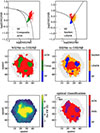 |
Fig. 1. Example of an optically selected AGN. In the top two panels, all the valid spaxels are plotted on the [N II]-based and [S II]-based BPT diagrams. In the middle panels, we show the 2D maps of how these spaxels are classified according to the BPT diagrams. In the lower-left panel, we show the Hα EW map. In the lower-right panel, we show the final spaxel-level classification, which combines all the information. |
For these optically selected AGNs, we derived L[OIII] based on the [O III] luminosity map and the spaxel-by-spaxel AGN classification map. To create the [O III] luminosity map, we first derived the uncorrected [O III] luminosity map from the pyPipe3D [O III] flux map. Dust attenuation was then corrected using the Balmer decrement measurements from Hα and Hβ flux maps, assuming the Calzetti (2001) dust extinction law with RV = 3.1, and an intrinsic Hα/Hβ ratio of 3.1 (Kewley et al. 2006). We then integrated [O III] luminosity over spaxels that were classified as AGN spaxels as the total L[OIII].
2.4. Spatially resolved measurements of star formation
To investigate star formation in the central regions, for all the MaNGA galaxies in our sample, we obtained the SFR surface density in the central 1 kpc region, ΣSFR, 1 kpc, in order to represent the absolute level of star formation. We also fully leveraged the MaNGA IFU data and obtained the radial profile of SFR density (see Sect. 2.4.1). We also combined the ΣSFR map and the Σ★ map to calculate the spaxel-by-spaxel deviation from the spatially resolved star formation main sequence (MS) and derive the radial profile of this deviation (see Sect. 2.4.2). In addition, we produced the map of Dn4000 and obtained the spatial profiles, which are closely related to age and can be utilized as another independent tracer of star formation properties (see Sect. 2.4.3).
2.4.1. ΣSFR measurements
We derived ΣSFR using the spatially resolved decomposition of the stellar populations provided by the pyPipe3D analysis (Sánchez et al. 2016a, 2022), which gives the fractions of luminosity from 273 templates spanning 39 stellar ages (1 Myr – 14.1 Gyr) and 7 metallicities. We converted the luminosity fractions to stellar mass fractions using the mass-to-light ratios provided for each simple stellar population (SSP) model. We then summed up the mass fractions at a certain age (but with different metallicities), which gave us the integrated M★ at a certain age for each spaxel. This allowed us to derive the SFR for each spaxel. The SFRssp adopted throughout this work is the average SFR within ∼100 Myr, which was calculated by adding all the masses with ages ≲ 100 Myr and then dividing by the time:
 (1)
(1)
As stated in Sánchez et al. (2016b), stellar population parameters obtained from SSP decomposition (e.g., age and metallicity) for MaNGA galaxies typically have uncertainties of 0.1–0.2 dex estimated from Monte Carlo simulations. The Monte Carlo uncertainty in M★ derived from SSP decomposition is typically comparable to that of these parameters (e.g. Cid Fernandes et al. 2014). These small uncertainties provide a reasonable basis for SSP-based SFR measurements, although the precision of such measurements naturally degrades in the regime of very old stellar populations. We also note that these Monte Carlo uncertainties reflect the statistical errors propagated from the flux measurement uncertainties through the fitting procedure, and do not include systematic effects. For SFR measurements, a significant portion of the uncertainty arises from the adopted SSP templates, along with other systematic uncertainties related to dust attenuation and star formation history parameterization. By comparing with SFR values estimated from Hα emission, the scatter of SSP-based SFR values is found to be around 0.3 dex (Sánchez et al. 2022), which demonstrates the general reliability of this type of measurement, considering that SFR averaged over the recent 100 Myr can be very sensitive to star formation history priors and difficult to constrain precisely (e.g. Leja et al. 2019). We further divided SFRssp per spaxel by the area per spaxel to get ΣSFR measurements.
To obtain ΣSFR, 1 kpc, we adopted the Sérsic profiles measured in the NASA-Sloan Atlas (NSA) catalog (Blanton et al. 2011) and created elliptical apertures with a major axis of 1 kpc and calculated the mean ΣSFR within the aperture2. When measuring the radial profile of ΣSFR, we also took elliptical apertures with different major axis sizes and used the mean ΣSFR of all the spaxels within different elliptical annuli. For all the ΣSFR measurements, including ΣSFR, 1 kpc measurements, we adopted the inclination correction suggested in Hsieh et al. (2017).
2.4.2. Deviation from the spatially resolved star formation MS
We obtained Σ★ maps utilizing the stellar mass maps provided by the pyPipe3D data products, which are also estimated from SSP decomposition. By comparing with M★ values estimated from multi-band photometry, the uncertainty of SSP-based M★ measurements is found to be around 0.2 dex (Sánchez et al. 2022), suggesting the general reliability of this type of measurement. We then measured the Σ★ radial profiles and Σ1 by taking the mean value of spaxels within the elliptical apertures or annuli with different major axis sizes, with inclination correction performed following Hsieh et al. (2017). Following the spatially resolved star formation MS obtained in Hsieh et al. (2017), log ΣSFR = 0.715 × log Σ★ − 8.065, we derived the deviation from this MS (ΔMS) for each spaxel, which enabled us to calculate the radial profile of ΔMS.
2.4.3. Dn4000 measurements
The strength of the 4000 Å break, Dn4000, is defined as the ratio of the average flux density in the narrow continuum bands 4000–4100 Å and 3850–3950 Å. Dn4000 closely tracks the stellar population age, and can also serve as an indicator for specific SFR (sSFR) at Dn4000 ≲ 1.8 (e.g. Brinchmann et al. 2004; Spindler et al. 2018). To measure spatially resolved Dn4000 profiles, we utilized the Data Analysis Pipeline (DAP; Westfall et al. 2019) spectral fitting results, which include the best-fitting stellar continuum models without emission-line components for all the spaxels.
2.5. Sample properties
In Fig. 2, we plot all the galaxies in the sample on the SFR versus M★ plane and the ΣSFR, 1 kpc versus Σ1 plane. X-ray and optical AGNs are marked as labeled. While there is a considerable fraction of AGNs among SF galaxies, we can see that in terms of the spatially resolved star formation MS, the central 1 kpc regions of most AGNs and normal galaxies lie below it (see Sect. 4.3 for discussions).
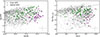 |
Fig. 2. Left: X-ray-selected AGNs and optically selected AGNs on the M★ versus SFR plane, as labeled. All galaxies in the sample are displayed as background points, with grayscale intensity encoding their weights. The error bar in the corner indicates uncertainties in M★ and SFR derived from pyPipe3D SSP decomposition, estimated by comparison with independent measurements (Sánchez et al. 2022). Right: Similar to the left panel, but for the Σ1 versus ΣSFR, 1 kpc plane. The dashed line depicts the spatially resolved star formation MS from Hsieh et al. (2017). The error bar in the corner indicates approximate uncertainty scales for Σ1 and ΣSFR, 1 kpc (see Footnote 2). |
In Fig. 3, we plot the X-ray/[O III] luminosities for X-ray/optical AGNs to approximate the accretion rate of these objects assuming a bolometric correction (e.g. Hopkins et al. 2007; Lamastra et al. 2009; Duras et al. 2020) and a radiative efficiency; in Fig. 4, we plot the LX/M★ and L[OIII]/M★ distributions, which can be used to approximate the specific black hole accretion rate (sBHAR), assuming M★ as a proxy for the BH mass. Most AGNs in our sample have log LX/M★ ≲ 31 and log L[OIII]/M★ ≲ 30. Following the conversion factor between LX/M★ and Eddington ratio reported in Eq. 2 of Aird et al. (2018) (which assumes a constant ratio between M★ and BH mass as well as a constant bolometric correction factor; see Aird et al. 2018 for details) and the average ratio of LX and L[OIII] reported in Lamastra et al. (2009), these values correspond to very weak accretion activity with Eddington ratios ≲ 0.1%.
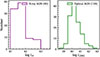 |
Fig. 3. Left: Log LX distribution of X-ray AGNs. LX represents the rest-frame 2–10 keV X-ray luminosity in units of erg s−1. Right: Log L[OIII] distribution of optical AGNs. L[OIII] represents the (extinction-corrected) luminosity of the [O III] λ5007 emission line in units of erg s−1. |
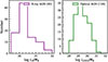 |
Fig. 4. Left: Log LX/M★ distribution of X-ray AGNs. Right: Log L[OIII]/M★ distribution of optical AGNs. LX/M★ and L[OIII]/M★ correspond to the X-ray and [O III] luminosity per unit stellar mass, respectively, in units of erg s−1 M⊙−1. |
As can be seen in Fig. 5, log LX and log L[OIII] as well as log LX/M★ and log L[OIII]/M★, are loosely correlated among objects that are identified as AGNs in both X-ray and optical bands. This indicates that the LX–L[OIII] relation is not merely driven by the tendency for more massive galaxies to exhibit higher LX and L[OIII] values, and we can compare the sBHAR of X-ray-selected AGNs and optically selected AGNs through a conversion—though with caution, as the scatter is significant (the measurement uncertainties of luminosities in this work may contribute substantially to the observed scatter, see Sect. 4.2 for discussions). Throughout the paper, we perform the analyses for X-ray AGNs and optical AGNs separately. Since we grouped X-ray AGNs into two categories with a cut at log LX/M★ = 30.5, we adopted a log L[OIII]/M★ cut of 29.5 for optical AGNs (which roughly corresponds to log LX/M★ = 30.5 given the Lamastra et al. (2009) relation represented in Fig. 5). We refer to X-ray AGNs with log LX/M★ > 30.5 as higher-LX/M★ AGNs, and those with log LX/M★ < 30.5 as lower-LX/M★ AGNs. Similarly, we refer to optical AGNs with log L[OIII]/M★ > 29.5 as higher-L[OIII]/M★ AGNs, and those with log L[OIII]/M★ < 29.5 as lower-L[OIII]/M★ AGNs. We do not directly refer to these subsamples as higher- or lower-sBHAR X-ray or optical AGNs because of the considerable scatter observed between log LX/M★ and log L[OIII]/M★, which comes from both the measurement uncertainty of these luminosities and the intrinsic uncertainty involved in using LX/M★ or L[OIII]/M★ as a proxy for the specific accretion rate (e.g. Aird et al. 2018; Duras et al. 2020; Suh et al. 2020). We also caution that most AGNs in the higher-LX/M★ or L[OIII]/M★ subsamples are still likely to have low Eddington ratios, as discussed in the paragraph above.
 |
Fig. 5. Left: LX versus L[OIII] for objects that are identified as both X-ray and optical AGNs. The dashed line shows the best-fit log LX–L[OIII] relation reported in Lamastra et al. (2009). Right: LX/M★ versus L[OIII]/M★ for objects that are identified as both X-ray and optical AGNs, with the best-fit relation converted from the log LX–L[OIII] relation. |
3. Analyses and results
3.1. AGN fraction as a function of central SFR density
3.1.1. X-ray-selected AGN fraction
In Fig. 6, we show how the X-ray AGN fraction varies as a function of ΣSFR, 1 kpc. To ensure that the contamination from other X-ray sources does not affect the results (see Sect. 2.2.4 for details), we studied log LX/M★ > 30.5 AGNs (i.e., higher-LX/M★ AGNs) only among objects with log M★ > 10.5 (that have X-ray coverage with LX, limit/M★ ≤ 30.5 as well), and log LX/M★ = 30–30.5 AGNs (i.e., lower-LX/M★ AGNs) only among galaxies with log M★ > 11 (also with LX, limit/M★ ≤ 30). We divided galaxies satisfying the above criterion into ΣSFR, 1 kpc bins with an equal number of objects per bin and then calculated the X-ray AGN fraction. When calculating the fraction, we adopted the weight reported in the MaNGA DAP catalog for each object to recover the results for a volume-limited sample3.
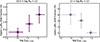 |
Fig. 6. Left: Fraction of X-ray AGNs with higher LX/M★ (log LX/M★ > 30.5) as a function of ΣSFR, 1 kpc, among objects with 10.5 < log M★ < 12. The y-axis error bars represent the 1σ confidence interval of AGN fraction from bootstrapping (i.e. randomly drawing the same number of objects from the sample 1000 times). The x-axis error bars represent the 16th and 84th percentiles of the ΣSFR, 1 kpc values. Right: Similar to the left panel, but for the fraction of lower-LX/M★ (log LX/M★ < 30.5) X-ray AGNs as a function of ΣSFR, 1 kpc, among objects with 11 < log M★ < 12. |
We can see that the higher-LX/M★ AGN fraction (with a median log LX/M★ ≈ 31) increases with ΣSFR, 1 kpc in the M★ range we probed. Due to the limited number of X-ray AGNs with relatively high LX/M★, we are only able to probe them in this large mass range. At the same time, among the most massive galaxies, the fraction of lower-LX/M★ AGNs (with even lower specific accretion rate, log LX/M★ = 30–30.5) decreases with ΣSFR, 1 kpc, in contrast to what has been observed for the fraction of higher-LX/M★ X-ray AGNs among galaxies with relatively smaller M★.
3.1.2. Optically selected AGN fraction
We further plot the fraction of optically selected AGNs as a function of ΣSFR, 1 kpc among galaxies in our sample. We studied two groups of optically selected AGNs: those with higher-L[OIII]/M★ values (log L[OIII]/M★ > 29.5) and those with relatively lower-L[OIII]/M★ values (log L[OIII]/M★ < 29.5), to roughly match the LX/M★ scales in Sect. 3.1.1 (see Sect. 2.5 for details). Although it is possible to estimate the [O III] flux upper limit for non-detections in individual spaxels, deriving L[OIII] requires integration over AGN spaxels. This is not possible when the classification itself is unavailable. Furthermore, even when an upper limit of L[OIII] can be estimated, proper decomposition is needed to truly estimate the AGN L[OIII] upper limit for weak AGNs among SF hosts (see Sect. 4.2). Giving an upper limit of L[OIII] for an optically selected AGN to be properly detected for each MaNGA galaxy is beyond the scope of this work, and we leave it for future work. We instead utilized all the galaxies as the parent sample, similar to previous MaNGA studies of optical AGNs. For optical AGNs in different L[OIII]/M★ groups, we studied them first in the large log M★ = 10.5–12 range following the approach in Sect. 3.1.1 (see Fig. 7), and then in smaller M★ bins to enable better comparison with the X-ray AGN sample (see Figs. 9 and 10).
 |
Fig. 7. Left: Fraction of higher-L[OIII]/M★ (log L[OIII]/M★ > 29.5) optical AGNs as a function of ΣSFR, 1 kpc, among objects with 10.5 < log M★ < 12. The y-axis error bars represent the 1σ confidence interval of AGN fraction from bootstrapping. The x-axis error bars represent the 16th and 84th percentiles of the ΣSFR, 1 kpc values. The gray shaded region represents the ΣSFR, 1 kpc range where optical AGN selection is considerably affected by contamination from star formation (see Sect. 4.1 for details). Right: Similar to the left panel, but for the fraction of lower-L[OIII]/M★ (log L[OIII]/M★ < 29.5) optical AGNs as a function of ΣSFR, 1 kpc among 10.5 < log M★ < 12 galaxies. |
We see that both the higher-L[OIII]/M★ and lower-L[OIII]/M★ optical AGN fractions increase with ΣSFR, 1 kpc when the ΣSFR, 1 kpc is small, but this increasing trend is not significantly present at the high-ΣSFR, 1 kpc end, especially for the lower- L[OIII]/M★ AGNs. When we group galaxies into more ΣSFR, 1 kpc bins (see Fig. 8), we can clearly observe a decreasing trend at the high-ΣSFR, 1 kpc end. If we study it in smaller M★ ranges (see Figs. 9 and 10), we can see that this decreasing trend is mostly associated with the log M★ = 10.5–11 objects. Among log M★ = 11–12 galaxies, the optical AGN fraction consistently increases with ΣSFR, 1 kpc. While it would be natural to conclude AGN negative feedback at a smaller mass range, we argue that it is actually more complicated, and discuss how selection effects come into play in Sect. 4.1. In all M★ and L[OIII]/M★ ranges, we do not observe an elevated optical AGN fraction among low-ΣSFR, 1 kpc galaxies as we observed for the lower-LX/M★ X-ray AGN fraction among massive galaxies (see the right panel of Fig. 6), and we discuss this in Sect. 4.1 as well.
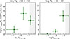 |
Fig. 9. Similar to Fig. 7, but for the fraction of higher-L[OIII]/M★ optical AGNs as a function of ΣSFR, 1 kpc among objects with 10.5 < log M★ < 11 (left) and objects with 11 < log M★ < 12 (right). |
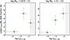 |
Fig. 10. Fraction of lower-L[OIII]/M★ optical AGNs as a function of ΣSFR, 1 kpc, among objects with 10.5 < log M★ < 11 (left) and objects with 11 < log M★ < 12 (right). |
3.2. Comparing the star-formation profiles of AGNs and normal galaxies with similar global properties
We also compare the full ΣSFR radial profiles of X-ray/optical AGNs with normal galaxies that share similar global properties. We have presented how AGN fraction is related to ΣSFR, 1 kpc, and we note that AGN fraction is related to global SFR as well. The full radial profile comparison will help to address whether the link between AGN activity and SFR in the galaxy’s central region is more than the manifestation of more AGNs among SF galaxies, and why this would be the case.
3.2.1. Profiles of X-ray-selected AGN hosts
Similar to the approach described in Sect. 3.1.1, we divided the X-ray AGNs into two categories: higher-LX/M★ (log LX/M★ > 30.5) AGNs among galaxies with log M★ = 10.5–12, and lower-LX/M★ (log LX/M★ = 30–30.5) AGNs only among galaxies with log M★ > 11.
When selecting normal galaxies to constitute the control sample, we limited our selection to galaxies with LX, limit/M★ smaller than the LX/M★ lower limit of the AGN sample. Furthermore, we excluded optical AGNs to make sure that the contamination in the control sample is as small as possible (we verified that our results did not change if we included optical AGNs in the control sample). For each X-ray AGN, we selected two normal galaxies with the closest M★, SFR, and z values utilizing the NearestNeighbors algorithm in the scikit-learn Python package. Then, for both the X-ray AGN sample and the control galaxy sample, we derived the mean radial profile of ΣSFR using elliptical annuli with a width of 1 kpc, extending out to 10 and 15 kpc for AGNs in the higher- and lower-LX/M★ samples, respectively, corresponding to ∼2 median Re for each sample. As can be seen in Fig. 11, higher-LX/M★ AGNs with log LX/M★ > 30.5 at log M★ = 10.5–12 show a steeper and more concentrated ΣSFR profile compared to normal galaxies when the total global SFR is roughly the same. In the central regions, higher-LX/M★ X-ray AGNs have higher ΣSFR, and the difference in ΣSFR is more prominent when the radius is small. In addition to the mean profile of ΣSFR, we also present the comparison of the mean Σ★, ΔMS, and Dn4000 profiles. We note that X-ray AGNs also have slightly higher Σ★ in the center – nevertheless, the differences in Σ★ profiles are not as significant as those in the ΣSFR profiles, as a lot of quiescent hosts are included in this study where Σ★ cannot trace the gas density very well. While both X-ray AGNs and normal galaxies show suppressed star formation relative to the spatially resolved star formation MS, as indicated by their mean ΔMS profiles, X-ray AGNs still show a mean ΔMS that is apparently high compared to normal galaxies in the central regions. In terms of Dn4000, we can see that X-ray AGNs are generally younger, and the difference is more prominent in the central regions (also indicating high sSFR when Dn4000 ≲ 1.8). As for the lower-LX/M★ AGNs (log LX/M★ = 30–30.5) among log M★ = 11–12 galaxies, their mean ΣSFR profile, ΔMS profile, and Σ★ profile do not show noticeable differences when compared with normal galaxies. At the same time, we can see that they have slightly younger cores and older outer regions.
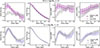 |
Fig. 11. Top: Mean ΣSFR, Σ★, ΔMS, Dn4000 profiles of higher-LX/M★ X-ray AGNs compared with normal galaxies in the control sample matched according to M★, SFR, and z individually, sampled with a 1 kpc interval in major-axis radius. Error bars represent the standard error of the mean. Bottom: Similar to the top panel, but for lower-LX/M★ X-ray AGNs. |
3.2.2. Profiles of optically selected AGN hosts
We grouped the optical AGNs into two L[OIII]/M★ groups as we did in Sect. 3.1.2, and we compared the profiles of higher- and lower-L[OIII]/M★ optical AGNs with those of normal galaxies following the approach described in Sect. 3.1.1. When constructing the control sample of normal galaxies, we also excluded all the defined X-ray AGNs to make sure that the contamination in the control sample is as small as possible (we verified that our results did not change qualitatively but became less prominent when we included X-ray AGNs in the control sample). The control sample was again constructed by selecting two normal galaxies with the closest M★, SFR, and z values. As can be seen in Fig. 12, both higher- and lower-L[OIII]/M★ AGNs show higher central ΣSFR compared to normal galaxies. They also exhibit higher central ΔMS compared to normal galaxies. Similar to X-ray AGN hosts, the differences in Σ★ profiles of optical AGN hosts compared with those of normal galaxies are not significant.
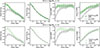 |
Fig. 12. Similar to Fig. 11, but for higher-L[OIII]/M★ optical AGNs (top) and lower-L[OIII]/M★ optical AGNs (bottom). |
4. Discussion
4.1. Missing optical AGNs among high-ΣSFR, 1 kpc galaxies and low-ΣSFR, 1 kpc galaxies
As can be seen in Figs. 7 and 8, the increasing trend of the optical AGN fraction with ΣSFR, 1 kpc is not present when the ΣSFR, 1 kpc is high. It is natural to link this with negative feedback, where AGNs are thought to be responsible for suppressing star formation in galaxy centers. However, before we know whether negative feedback is observed or not, we need to account for the bias associated with the BPT-based optical AGN selection method. Among SF areas, H II regions can produce emission lines that mimic AGN features, and when the AGN is relatively weak or is obscured, the AGN signal may be buried beneath the SF activity. For example, in the BPT diagram we utilized to identify the dominant source of ionization, SF spaxels with weak and/or obscured AGN signal may fall into the “ambiguous” and “SF” spaxels.
As suggested by the correlation between SFR and L[OIII] reported in Villa-Vélez et al. (2021),
![Mathematical equation: $$ \begin{aligned} \mathrm{log\ SFR = log}\ L_{\rm [O III]} - 41.2, \end{aligned} $$](/articles/aa/full_html/2026/08/aa57301-25/aa57301-25-eq2.gif) (2)
(2)
higher SFRs require a higher threshold for reliable AGN detection. This also works for the surface density of these values. We note that ≳90% of the optical AGNs in our sample have [O III] surface luminosity densities (ΣL[OIII]) in the central 1 kpc region of ≳1039.7 erg s−1 kpc−2. When ΣL[OIII] generated by the central star formation is comparable to that generated by the AGN, we consider it difficult to identify the AGN from the BPT diagram. This corresponds to log ΣSFR, 1 kpc ∼ −1.8. In reality, we note that AGNs identified via BPT diagrams typically contribute more to the total [O III] flux when they pass the classification line (e.g. Davies et al. 2014). There are also uncertainties associated with the log SFR–log L[OIII] relation: Villa-Vélez et al. (2021) noted that variations in metallicity and ionization parameters can theoretically lead to a spread of up to 1.1 dex; the empirical scatter of this relation reported ranges from ≈ 0.3 to 0.6 dex (e.g. Moustakas et al. 2006; Villa-Vélez et al. 2021). These indicate that the ΣSFR, 1 kpc threshold for an optical AGN to be very safely detected could be even lower. Given the contamination threshold, a fraction of optical AGNs may be missed in the highest ΣSFR, 1 kpc bin, so we cannot conclude negative feedback from this. For galaxies with log M★ = 10.5–11, most objects grouped into the highest ΣSFR, 1 kpc bin in Fig. 9 have log ΣSFR, 1 kpc values from −2.1 to −1.3. Thus, a significant fraction of AGNs in this bin are likely to suffer strongly from selection effects, contributing to the clear drop in the AGN fraction at the high-ΣSFR, 1 kpc end. For galaxies with log M★ = 11–12, most objects grouped into the highest ΣSFR, 1 kpc bin have log ΣSFR, 1 kpc values from −2.5 to −1.5. A large fraction of these objects are likely less affected by selection bias; thus, the increasing trend can be clearly observed. While AGNs with higher L[OIII] do not naturally translate into higher [O III] surface luminosity density, higher-L[OIII]/M★ AGNs are more likely to have higher ΣL[OIII]. Thus, we can see that the drop at the high-ΣSFR, 1 kpc end is more pronounced among optical AGNs with lower L[OIII]/M★.
Also, when we selected optical AGNs, we required the emission lines utilized in the study to have S/N > 3 and Hα EW > 3 Å. This naturally makes it difficult to classify weak and/or obscured AGNs, especially among quiescent galaxies with low ΣSFR, 1 kpc values. Thus, for optically selected AGNs in this study, we are not able to observe the elevated low-L[OIII]/M★ AGN fraction among low-ΣSFR, 1 kpc galaxies as we observed for X-ray-selected AGNs, leading to the observed discrepancy.
4.2. Is coeval growth in tension with AGN feedback?
Unlike optically selected AGNs, the fraction of higher-LX/M★ X-ray AGNs with log LX/M★ > 30.5 shows a steadily increasing trend with ΣSFR, 1 kpc (see the left panel of Fig. 6), consistent with the expectation from the coeval growth picture arising from the common origin of gas in the vicinity of the BH and in the central region of galaxies. We note that X-ray selection is not completely safe from missing obscured AGNs, especially since a fraction of sources were selected in the eROSITA sky coverage, which is mainly sensitive in the soft band rather than the hard band (the obscuration effect is minimized in the hard band). If we consider that the obscuration level of AGN structure itself (e.g., torus) does not vary significantly with ΣSFR, 1 kpc, the obscuration level from the host-galaxy component (which also leads to considerable obscuration; e.g., Goulding et al. 2018; Gilli et al. 2022) could increase with ΣSFR, 1 kpc. As the increasing trend is present even with potential obscuration bias, we consider the picture of common fuel and coeval growth to be stable. If we look at the Dn4000 profiles (see the top panel of Fig. 11), we can see that these higher-LX/M★ X-ray AGNs, as well as all the optical AGNs with higher L[OIII]/M★ (see Fig. 12), generally have younger stellar populations compared to galaxies with similar M★ and SFR, suggesting different star formation histories; that is, galaxies that host these AGNs are more likely to have more recent star formation episodes so that the average age appears lower, and the cold gas replenishment also triggers AGN activity.
Due to the limited sample size, we cannot statistically prove how significant ΣSFR, 1 kpc is as an indicator of AGN activity or BH growth compared to total SFR. However, analysis results in Figs. 11 and 12 already demonstrate that the link between AGN activity and ΣSFR, 1 kpc is more than simply manifesting the link between AGN activity and global SFR, as these AGNs and control galaxies have similar global SFRs. In Ni et al. (2021), we found that the projected central surface mass density within 1 kpc, Σ1, is more effective in predicting the BH growth level compared to other compactness parameters among SF galaxies. This can be understood at a phenomenological level from the slope of the ΣSFR radial profiles: the differences between AGNs and normal galaxies in ΣSFR, and thus in the available gas fuel, are more prominent in the central regions.
However, there is well-established observational evidence that AGNs can evacuate gas in the central regions of galaxies (e.g., García-Burillo et al. 2014; Fluetsch et al. 2019; Parlanti et al. 2025), so one would naturally expect reduced ΣSFR, 1 kpc in these cases. This raises the question of how these results can be consistent with a higher AGN fraction among galaxies with higher levels of central star formation.
In Fig. 13, instead of comparing the mean ΣSFR profiles of X-ray AGNs and matched normal galaxies as a function of major-axis radius, we show the distribution of the difference in log ΣSFR (Δ log ΣSFR; log ΣSFR (AGN) − log ΣSFR (control galaxy) at the individual level) at different radii. Similar to the obvious difference in mean log ΣSFR as shown in Fig. 11, the median log ΣSFR of X-ray AGNs is also higher in the central regions. At the same time, the wide distribution of Δlog ΣSFR suggests the unreliability of deriving a universal conclusion for the AGN feedback scenario via a limited number of objects, particularly a single observation (which has been a widely adopted approach), as it will easily lead to a conclusion of positive or negative feedback—which could be at play for this particular object but not all the others. When considering the overall trend, while we attribute the link between AGN incidence and higher central ΣSFR (on average) to coeval growth from a common fuel supply, the wide distribution of Δ log ΣSFR can be attributed to various factors.
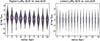 |
Fig. 13. Left: Violin plot showing the distribution of differences in ΣSFR between higher-LX/M★ AGNs and matched control galaxies at each radius. Similar to the mean ΣSFR profiles presented in Fig. 11, clear differences in the medians are also observed, especially in the central regions. However, the distributions of Δ log ΣSFR for individual matched pairs remain broad, spanning both positive and negative values. Right: Similar to the left panel, but for lower-LX/M★ AGNs. The Δ log ΣSFR distributions are also broad, while no clear differences in the medians are observed in galaxy central regions (aligning with the lack of significant differences in the mean ΣSFR profiles). |
We first need to account for AGN variability. The X-ray luminosity of AGNs can vary by orders of magnitude over a Myr timescale (e.g. Hickox et al. 2014), and the SFR we adopted in this study is measured over even longer timescales. The observed X-ray AGNs with a certain LX/M★ criterion might not fulfill this criterion over most of the time during which the SFR is estimated; similarly, the normal galaxy used for comparison might be an X-ray AGN in recent history. While L[OIII] also exhibits variability and is subject to the same timescale effect mentioned above, compared with the X-ray emission, [O III] emission is much closer to a long-term average measurement, as it comes from the NLR that is further away from the central supermassive BH (on a ∼104–105 light-year scale) and has an extended spatial distribution. In this case, one would expect smaller scatters of the Δlog ΣSFR compared to normal galaxies, if variability plays a smaller role here. We do observe that the scatter is slightly smaller, particularly at the central radii. However, the scatter is still considerable, which might be related to the optical AGN selection bias in this study (see Sect. 4.1), so some unclassified AGNs may remain in the matched control galaxy sample.
In addition, there might be real hints of feedback in action. It has been argued that negative feedback on star formation is most efficient in powerful AGNs (e.g. Cicone et al. 2014), as the powerful AGN winds could blow out gas in the central regions and stop the gas from fragmentation (e.g. Zubovas & Bourne 2017). For AGNs that are not especially luminous, such as objects in our sample, small-scale outflows can inject turbulence into the ISM, and/or heat the gas, thus also weakening the star formation, especially in the central region (e.g. Parlanti et al. 2025). At the same time, positive AGN feedback is also predicted and observed, whereby the ISM is compressed and the SFR is enhanced (e.g. Maiolino et al. 2017; Shin et al. 2019). We cannot confidently argue that we have observed strong evidence for positive AGN feedback, as the overall elevated ΣSFR spans areas larger than what AGNs at this low level of luminosity can impact. However, we might have observed evidence for negative AGN feedback, though very slight, as the ΣSFR profiles in Figs. 11 and 12 show either a small decline in the central few kiloparsecs (though this decline is small compared to the absolute value of ΣSFR), or a flattening of the inwardly increasing trend within the central few kiloparsecs. Under the negative AGN feedback scenario, one might expect more extended tails toward negative Δlog ΣSFR and a smaller median Δlog ΣSFR value in the central region among higher-L[OIII]/M★ optical AGNs compared to lower-L[OIII]/M★ optical AGNs in Fig. 14, if more powerful AGNs launch more powerful outflows. We observe slightly more extended negative Δlog ΣSFR tails over the central region among lower-L[OIII]/M★ optical AGNs. However, we note that the selection effect also plays a role in optical AGN identification as discussed earlier, and the differences are not significant; therefore, from these plots, we cannot reliably test whether central star formation suppression is more pronounced among AGN hosts with higher AGN luminosities. Also, we note that L[OIII] obtained from summing over the [O III] flux reported in pyPipe3D data products in AGN-dominated spaxels may not be a robust indicator of the true AGN luminosity. As we have discussed, weak or obscured AGN emission is hard to distinguish from the emission lines associated with SF activity; also, AGN outflows can broaden the [O III] emission line, and the shifted wings may contribute significantly, but they are not accounted for correctly given the current pyPipe3D line-measurement method (a single Gaussian fitting; Sánchez et al. 2016a). Thus, our subsamples divided according to L[OIII]/M★ might not distinguish true specific accretion power very clearly, which is also shown in Fig. 4 – a better measurement of the L[OIII] from the AGN will help to further investigate the negative AGN feedback scenario, if objects with higher- and lower-sBHAR are better separated.
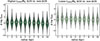 |
Fig. 14. Similar to Fig. 13, but for higher-L[OIII]/M★ optical AGNs (left) and lower-L[OIII]/M★ optical AGNs (right). Consistent with the clear differences in the mean ΣSFR profiles presented in Fig. 12, offsets in the median values of the distributions (indicated by short horizontal lines) are observed for both groups in the central regions of galaxies. The overall distributions of Δ log ΣSFR for individual matched pairs are broad, extending significantly into both positive and negative values. |
Among massive galaxies with log M★ > 11, we observe a decreasing trend of notably low sBHAR (log LX/M★ < 30.5) AGNs with increasing ΣSFR, 1 kpc (see the right panel of Fig. 6). We interpret this as being associated with both large M★ and the low sBHAR, where stochastic fueling from condensed hot halo gas serves as the major fuel. Hot halo gas fueling has long been proposed as a source for powering low-sBHAR AGNs, and both the trend of increasing low-sBHAR radio AGN fraction and X-ray AGN fraction with M★ has been observed among massive galaxies (e.g. Best & Heckman 2012; Ni et al. 2023). Among massive galaxies with log M★ > 11, lower ΣSFR, 1 kpc is indeed associated with galaxies with higher M★ and older stellar populations. These galaxies tend to reside in larger halos (e.g. Wechsler & Tinker 2018), which also contain more fuel to power AGNs with low levels of accretion activity through the stochastic condensation of halo gas, so that an elevated lower-LX/M★ AGN fraction is observed at the low-ΣSFR, 1 kpc end. For galaxies with similar M★, older galaxies tend to form earlier in more massive halos (e.g. Rodríguez-Puebla et al. 2015; Wechsler & Tinker 2018) that have more fuel for the central BH. This explains why log LX/M★ < 30.5 AGN hosts on average have older stellar populations in the outskirts compared to matched normal galaxies (see the bottom panel of Fig. 11), which is consistent with their formation history. They also have younger cores as a result of a slightly enhanced level of central star formation fueled by a larger reservoir of condensed halo gas. We also do not observe an obvious difference in the mean ΣSFR profiles of these X-ray AGNs and normal galaxies (see Fig. 11). We note that the SFR in this study was derived based on decomposing the stellar continuum (see Sect. 2.4.1), which is not very sensitive to a small level of very recent star formation (at the ∼10 Myr scale) when the overall stellar population is old. ΣSFR derived from SSP decomposition is more stable for the average SFR over a longer period, such as the 100 Myr scale used in this study. Higher levels of Hα emission can indeed be observed among these massive AGN hosts that cannot fully be attributed to AGN emission, indicating very weak star formation activity (which supports that what fuels the AGN must fuel the galaxy at the same time, to some extent) that becomes hard to detect when averaged out to longer timescales (see Fig. 15)4. In general, we observe more low-LX/M★ AGNs among galaxies with low ΣSFR, 1 kpc, which depleted their cold gas earlier but have more hot halo gas fuel available. Also, compared to the mean ΣSFR profiles of higher-LX/M★ AGNs among less massive galaxies, the mean ΣSFR profile of massive log LX/M★ < 30.5 AGN hosts shows a larger decline in the central ≲ 3 kpc region. For low-accretion-rate AGNs among massive galaxies, jet activity is considered to be very prevalent (e.g. Best et al. 2005). AGN jets are known to be a key mechanism for maintenance-mode AGN feedback, during which the surrounding gas is heated and disturbed, and cannot cool and form stars efficiently. Simulation results (e.g. Gaibler et al. 2012) predict that jets can create a small cavity in the galaxy center (≲ 3 kpc) and increase the SFR in the outer regions; these effects might explain the central ΣSFR decline we observed among massive log LX/M★ < 30.5 AGN hosts that is more noticeable (in both scale and amplitude) compared to that among other AGN hosts. While a single AGN active episode is short, the cavities left behind can persist on timescales comparable to those over which the SSP-based SFR is estimated (∼ 100 Myr). In the bottom panel of Fig. 11, we see the central ΣSFR decline almost equally in terms of AGNs and non-AGNs, which would be consistent with the effects of AGN jet-mode feedback on the relevant timescales.
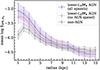 |
Fig. 15. SFR surface density profiles estimated from Hα, of X-ray AGNs with lower LX/M★ (log LX/M★ < 30.5) and normal galaxies utilized in Fig. 11. We can see that even the mean ΣSFR estimated from Hα emission from spaxels that are not AGN-dominated is elevated compared to that of non-AGNs in the control galaxy sample, suggesting that a minute level of SF enhancement is likely among the hosts of these very weak AGNs, when we select an SF indicator that is sensitive to very recent SF activity. |
4.3. Comparison with previous studies
In Fig. 16, we plot the mean ΔMS profiles as well as the specific SFR surface density (ΣsSFR) profiles of all the galaxies in the sample grouped into different M★ and SFR bins. We can see that galaxies in the MaNGA sample have suppressed central star formation properties on average, while most of them do not host detectable AGNs5. Thus, it is not surprising to observe suppressed SFRs among AGN hosts (e.g. Acharya et al. 2024) or low gas fractions among AGN regions (e.g. Ellison et al. 2021); galaxies at low redshift have suppressed centers on average, and AGN regions are just located in the centers. A causal relation between AGN feedback and the suppression of central SFR concluded this way needs further caution.
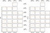 |
Fig. 16. Left: Mean ΔMS profiles of all the galaxies in the sample grouped according to their M★ and SFR values. Error bars represent the standard error of the mean. Right: Similar to the left panel, but for ΣsSFR profiles. |
Even when the control galaxies are selected, if one does not take into account the limitation of optical AGN selection bias, suppressed central SFRs can be observed among some subsamples (e.g. Bing et al. 2019; Lammers et al. 2023; Gatto et al. 2025). Also, the effects of high global SFR and high central SFR in predicting the high level of AGN activity are hard to disentangle when control galaxies are selected only based on M★. In Fig. 17, we plot the mean ΣSFR profiles for all the galaxies in the sample, grouped according to M★ and SFR values. We can see that for a given M★, when the global SFR is high, the profiles are more centrally concentrated. This effect is more prominent among log M★ < 11 galaxies, where the ΣSFR profiles become flatter when the global SFR decreases, and ΣSFR values in the central regions go through much larger variations compared to ΣSFR in the outer regions. This is consistent with the expectation of cold gas supply distributed according to the host-galaxy potential well. Among the most massive galaxies, we can see signs of elevated ΣSFR in the central regions that do not relate to fueling at the global scale. Together, these factors point to the need to select control galaxies with similar SFR values rather than simply controlling for M★ when studying how the central star formation property, in particular, relates to AGN activity: if one does not control for SFR (e.g. Bing et al. 2019; Mulcahey et al. 2022; Lammers et al. 2023; Acharya et al. 2024; Gatto et al. 2025), there might be a higher risk of observing artificially suppressed ΣSFR among AGN hosts due to the selection effects as we previously discussed. In our work, we also observe the decreasing optical AGN fraction at the high-ΣSFR, 1 kpc end, but since we controlled for the global SFR when comparing the ΣSFR profiles (the significance of the selection effect varies as a function of both ΣSFR, 1 kpc and total SFR), the high central ΣSFR of optical AGNs compared to normal galaxies can also be observed (though the true difference might be larger, as there are still missing optical AGNs expected among control galaxies). Furthermore, by controlling for the global SFR as well as M★ through the nearest-neighbour method, we can reliably observe how AGN activity is connected to the availability of gas supply in the center of the galaxy (or the distribution of the gas supply) when the total global gas supply is comparable rather than there simply being more gas in the center when there is more available throughout the whole galaxy.
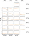 |
Fig. 17. Mean ΣSFR profiles of galaxies in the sample grouped according to their M★ and SFR values. Error bars represent the standard error of the mean. |
We therefore advise caution in interpreting previous studies that yield different results in central star formation differences when comparing AGNs with different luminosities to normal galaxies. First, as we discussed in Sect. 4.2, emission-line luminosity cannot safely probe AGN luminosity among low-to-moderate-luminosity AGNs, which is also a challenge for radio luminosity measurements (e.g. Mulcahey et al. 2022; Gatto et al. 2025). Estimation from the X-ray emission, as adopted in the study, is relatively safer, but only when the contamination from the XRB is small. This is also the limitation of the X-ray selection, as the nature of galaxies with log LX < 41 would be hard to justify, and results established for this type of subsample (e.g. Acharya et al. 2024) should be treated with caution6. Second, similar luminosity cannot represent a similar AGN accretion level when probing galaxies with a large range of BH masses, and adding the normalization from M★ can better approximate the specific accretion rate. Last but not least, we caution that different mean ΣSFR and/or ΣsSFR profiles of AGNs with different luminosity levels (which is commonly adopted in previous studies) or even specific accretion rates do not necessarily mean that their host galaxies are different. Assuming a relatively similar accretion rate distribution throughout the galaxy population (e.g. Aird et al. 2019), one might find that AGNs with higher luminosities or accretion rates have higher ΣSFR, 1 kpc among a limited-size sample, given that the probability of detecting such an AGN among low-ΣSFR, 1 kpc galaxies is very low. It is plausible that the specific accretion rate distribution of AGNs varies with ΣSFR, 1 kpc; however, due to the limited sample size of the work, we cannot probe it confidently, and given the results from Aird et al. (2019) that the average specific accretion rate does not vary significantly with SFR at low redshift, which correlates with ΣSFR, 1 kpc, one might not expect dramatic variation in the specific accretion rate distribution across different ΣSFR, 1 kpc ranges (except for extreme ΣSFR, 1 kpc values).
5. Conclusions
Utilizing the IFU spectroscopy from SDSS MaNGA, we studied how X-ray and optical AGN fractions vary as a function of ΣSFR, 1 kpc and investigated the spatially resolved properties of X-ray and optical AGN hosts compared to normal galaxies. The main points from this paper can be summarized as follows:
-
We built a sample of MaNGA galaxies that have X-ray coverage from eROSITA, XMM-Newton, or Chandra, and identified X-ray AGNs (see Sect. 2.2) and optical AGNs (see Sect. 2.3) among this sample. For all the objects in the sample, we constructed Σ★, ΣSFR, ΔMS, and Dn4000 maps to derive the corresponding radial profiles, and obtained the ΣSFR, 1 kpc measurements (see Sect. 2.4).
-
We studied the fractions of X-ray and optical AGNs as a function of ΣSFR, 1 kpc (see Sect. 3.1). We found that the fraction of log LX/M★ > 30.5 AGNs increases with ΣSFR, 1 kpc, while the fraction of log LX/M★ < 30.5 AGNs decreases with ΣSFR, 1 kpc among log M★ > 11 galaxies where these X-ray AGNs with negligible levels of accretion can be detected (see Sect. 3.1.1). The optical AGN fraction typically increases with ΣSFR, 1 kpc, while there is a drop at the high ΣSFR, 1 kpc end that is more prominent when the probed M★ range is smaller (see Sect. 3.1.2).
-
We further studied the spatially resolved profiles of X-ray/optical AGN hosts and compared them with those of galaxies matched with similar global properties: log M★, log SFR, and z (see Sect. 3.2). We found that both X-ray and optical AGNs tend to have higher central ΣSFR, though log LX/M★ < 30.5 AGNs do not show significant differences in central ΣSFR compared with normal galaxies when the method for measuring ΣSFR is not sensitive to very recent star formation (see Sect. 3.2.1).
-
We argue that the observed discrepancy in the results among X-ray AGNs and optical AGNs can be attributed to selection effects. In addition to the well-known limitation of optical selection in picking up weak AGNs among quiescent galaxies, as identifying weak AGNs with BPT diagrams becomes harder when the star formation activity is stronger, one might observe a drop in the optically selected AGN fraction at the high-ΣSFR, 1 kpc end, which might be misinterpreted as negative AGN feedback (see Sect. 4.1).
-
The elevated level of central ΣSFR among AGN hosts we observed is generally consistent with the picture of coeval growth of BHs and central parts of galaxies as a result of a common fuel supply; the difference in ΣSFR is more prominent in the inner regions, which could explain why BH growth is more closely related to host-galaxy properties in the central kiloparsec regions (see Sect. 4.2). While most of the massive galaxies in the local Universe have suppressed sSFR in the center (which can also be misinterpreted as evidence for negative AGN feedback), lower levels of central ΣSFR of AGN hosts compared to normal galaxies on average should not be observed if the AGN and control galaxy samples are carefully selected (see Sect. 4.3).
-
We also note that the picture of coeval growth from a common fuel supply does not contradict AGN feedback in action. For individual objects, it is possible to observe the effects of both positive and negative AGN feedback. We can also observe slight decreases (or flattening) of the mean ΣSFR profiles toward the galaxy center on small scales (≲ several kiloparsecs) among AGN hosts in our sample, consistent with the expectation that AGN feedback can suppress star formation (e.g., via outflows); these features do not contradict our overall finding that AGN hosts in our sample exhibit, on average, elevated central ΣSFR. Among the most massive galaxies, this decreasing trend becomes more noticeable (in both scale and amplitude), consistent with the expectation of jet-related AGN feedback (see Sect. 4.2).
In the future, the accumulation of JWST IFU observations will help to extend the analyses to higher redshifts, where a population of more powerful AGNs can be probed among galaxies with more active star formation, and the dynamic balance between fueling and feedback in the common gas reservoir will have larger variations, so that both effects can be observed more clearly. Combining jet and outflow properties of AGNs into this type of analysis will also help to test the scenario proposed in this study.
Acknowledgments
We thank the anonymous referee for constructive feedback. This work is based on data from eROSITA, the soft X-ray instrument aboard SRG, a joint Russian-German science mission supported by the Russian Space Agency (Roskosmos), in the interests of the Russian Academy of Sciences represented by its Space Research Institute (IKI), and the Deutsches Zentrum für Luft- und Raumfahrt (DLR). The SRG spacecraft was built by Lavochkin Association (NPOL) and its subcontractors, and is operated by NPOL with support from the Max Planck Institute for Extraterrestrial Physics (MPE). The development and construction of the eROSITA X-ray instrument was led by MPE, with contributions from the Dr. Karl Remeis Observatory Bamberg & ECAP (FAU Erlangen-Nuernberg), the University of Hamburg Observatory, the Leibniz Institute for Astrophysics Potsdam (AIP), and the Institute for Astronomy and Astrophysics of the University of Tübingen, with the support of DLR and the Max Planck Society. The Argelander Institute for Astronomy of the University of Bonn and the Ludwig Maximilians Universität Munich also participated in the science preparation for eROSITA. The eROSITA data shown here were processed using the eSASS/NRTA software system developed by the German eROSITA consortium.
References
- Acharya, N., Bonoli, S., Salvato, M., et al. 2024, A&A, 687, A285 [NASA ADS] [CrossRef] [EDP Sciences] [Google Scholar]
- Aird, J., Coil, A. L., & Georgakakis, A. 2018, MNRAS, 474, 1225 [NASA ADS] [CrossRef] [Google Scholar]
- Aird, J., Coil, A. L., & Georgakakis, A. 2019, MNRAS, 484, 4360 [NASA ADS] [CrossRef] [Google Scholar]
- Albán, M., & Wylezalek, D. 2023, A&A, 674, A85 [NASA ADS] [CrossRef] [EDP Sciences] [Google Scholar]
- Alexander, D. M., & Hickox, R. C. 2012, New Astron. Rev., 56, 93 [Google Scholar]
- Andonie, C., Alexander, D. M., Greenwell, C., et al. 2024, MNRAS, 527, L144 [Google Scholar]
- Best, P. N., & Heckman, T. M. 2012, MNRAS, 421, 1569 [NASA ADS] [CrossRef] [Google Scholar]
- Best, P. N., Kauffmann, G., Heckman, T. M., et al. 2005, MNRAS, 362, 25 [Google Scholar]
- Bing, L., Shi, Y., Chen, Y., et al. 2019, MNRAS, 482, 194 [NASA ADS] [CrossRef] [Google Scholar]
- Birchall, K. L., Watson, M. G., Aird, J., & Starling, R. L. C. 2022, MNRAS, 510, 4556 [NASA ADS] [CrossRef] [Google Scholar]
- Blanton, M. R., Kazin, E., Muna, D., Weaver, B. A., & Price-Whelan, A. 2011, AJ, 142, 31 [NASA ADS] [CrossRef] [Google Scholar]
- Brinchmann, J., Charlot, S., White, S. D. M., et al. 2004, MNRAS, 351, 1151 [Google Scholar]
- Bryant, J. J., Owers, M. S., Robotham, A. S. G., et al. 2015, MNRAS, 447, 2857 [Google Scholar]
- Bundy, K., Bershady, M. A., Law, D. R., et al. 2015, ApJ, 798, 7 [Google Scholar]
- Calzetti, D. 2001, PASP, 113, 1449 [Google Scholar]
- Chen, C.-T. J., Hickox, R. C., Alberts, S., et al. 2013, ApJ, 773, 3 [NASA ADS] [CrossRef] [Google Scholar]
- Cicone, C., Maiolino, R., Sturm, E., et al. 2014, A&A, 562, A21 [NASA ADS] [CrossRef] [EDP Sciences] [Google Scholar]
- Cid Fernandes, R., Stasińska, G., Mateus, A., & Vale Asari, N. 2011, MNRAS, 413, 1687 [Google Scholar]
- Cid Fernandes, R., González Delgado, R. M., García Benito, R., et al. 2014, A&A, 561, A130 [NASA ADS] [CrossRef] [EDP Sciences] [Google Scholar]
- Croton, D. J., Springel, V., White, S. D. M., et al. 2006, MNRAS, 365, 11 [Google Scholar]
- Davies, R. L., Kewley, L. J., Ho, I.-T., & Dopita, M. A. 2014, MNRAS, 444, 3961 [NASA ADS] [CrossRef] [Google Scholar]
- Duras, F., Bongiorno, A., Ricci, F., et al. 2020, A&A, 636, A73 [NASA ADS] [CrossRef] [EDP Sciences] [Google Scholar]
- Ellison, S. L., Wong, T., Sánchez, S. F., et al. 2021, MNRAS, 505, L46 [NASA ADS] [CrossRef] [Google Scholar]
- Evans, I. N., Evans, J. D., Martínez-Galarza, J. R., et al. 2024, ApJS, 274, 22 [NASA ADS] [CrossRef] [Google Scholar]
- Fabian, A. C. 2012, ARA&A, 50, 455 [Google Scholar]
- Fluetsch, A., Maiolino, R., Carniani, S., et al. 2019, MNRAS, 483, 4586 [NASA ADS] [Google Scholar]
- Fragos, T., Lehmer, B. D., Naoz, S., Zezas, A., & Basu-Zych, A. 2013, ApJ, 776, L31 [CrossRef] [Google Scholar]
- Fu, Y., Cappellari, M., Mao, S., et al. 2023, MNRAS, 524, 5827 [CrossRef] [Google Scholar]
- Gaibler, V., Khochfar, S., Krause, M., & Silk, J. 2012, MNRAS, 425, 438 [NASA ADS] [CrossRef] [Google Scholar]
- García-Burillo, S., Combes, F., Usero, A., et al. 2014, A&A, 567, A125 [Google Scholar]
- Gatto, L., Storchi-Bergmann, T., Riffel, R. A., et al. 2025, MNRAS, 539, 3229 [Google Scholar]
- Gilli, R., Norman, C., Calura, F., et al. 2022, A&A, 666, A17 [NASA ADS] [CrossRef] [EDP Sciences] [Google Scholar]
- Goulding, A. D., Greene, J. E., Bezanson, R., et al. 2018, PASJ, 70, S37 [NASA ADS] [CrossRef] [Google Scholar]
- Harrison, C. M. 2017, Nat. Astron., 1, 0165 [NASA ADS] [CrossRef] [Google Scholar]
- Hickox, R. C., & Alexander, D. M. 2018, ARA&A, 56, 625 [Google Scholar]
- Hickox, R. C., Mullaney, J. R., Alexander, D. M., et al. 2014, ApJ, 782, 9 [NASA ADS] [CrossRef] [Google Scholar]
- Hopkins, P. F., Richards, G. T., & Hernquist, L. 2007, ApJ, 654, 731 [Google Scholar]
- Hsieh, B. C., Lin, L., Lin, J. H., et al. 2017, ApJ, 851, L24 [Google Scholar]
- Kennicutt, R. C., Jr. 1998, ARA&A, 36, 189 [Google Scholar]
- Kewley, L. J., Groves, B., Kauffmann, G., & Heckman, T. 2006, MNRAS, 372, 961 [Google Scholar]
- Kormendy, J., & Ho, L. C. 2013, ARA&A, 51, 511 [Google Scholar]
- Lamastra, A., Bianchi, S., Matt, G., et al. 2009, A&A, 504, 73 [NASA ADS] [CrossRef] [EDP Sciences] [Google Scholar]
- Lammers, C., Iyer, K. G., Ibarra-Medel, H., et al. 2023, ApJ, 953, 26 [NASA ADS] [CrossRef] [Google Scholar]
- Law, D. R., Cherinka, B., Yan, R., et al. 2016, AJ, 152, 83 [Google Scholar]
- Lehmer, B. D., Basu-Zych, A. R., Mineo, S., et al. 2016, ApJ, 825, 7 [Google Scholar]
- Leja, J., Carnall, A. C., Johnson, B. D., Conroy, C., & Speagle, J. S. 2019, ApJ, 876, 3 [Google Scholar]
- Maiolino, R., Russell, H. R., Fabian, A. C., et al. 2017, Nature, 544, 202 [Google Scholar]
- Mineo, S., Gilfanov, M., & Sunyaev, R. 2012, MNRAS, 426, 1870 [NASA ADS] [CrossRef] [Google Scholar]
- Moustakas, J., Kennicutt, R. C., Jr, & Tremonti, C. A. 2006, ApJ, 642, 775 [NASA ADS] [CrossRef] [Google Scholar]
- Mulcahey, C. R., Leslie, S. K., Jackson, T. M., et al. 2022, A&A, 665, A144 [NASA ADS] [CrossRef] [EDP Sciences] [Google Scholar]
- Ni, Q., Yang, G., Brandt, W. N., et al. 2019, MNRAS, 490, 1135 [NASA ADS] [CrossRef] [Google Scholar]
- Ni, Q., Brandt, W. N., Yang, G., et al. 2021, MNRAS, 500, 4989 [Google Scholar]
- Ni, Q., Aird, J., Merloni, A., et al. 2023, MNRAS, 524, 4778 [CrossRef] [Google Scholar]
- Oh, K., Yi, S. K., Schawinski, K., et al. 2015, ApJS, 219, 1 [Google Scholar]
- Parlanti, E., Carniani, S., Venturi, G., et al. 2025, A&A, 695, A6 [NASA ADS] [CrossRef] [EDP Sciences] [Google Scholar]
- Predehl, P., Andritschke, R., Arefiev, V., et al. 2021, A&A, 647, A1 [EDP Sciences] [Google Scholar]
- Rodríguez-Puebla, A., Avila-Reese, V., Yang, X., et al. 2015, ApJ, 799, 130 [Google Scholar]
- Ruiz, A., Georgakakis, A., Gerakakis, S., et al. 2022, MNRAS, 511, 4265 [NASA ADS] [CrossRef] [Google Scholar]
- Salpeter, E. E. 1955, ApJ, 121, 161 [Google Scholar]
- Sánchez, S. F., Kennicutt, R. C., Gil de Paz, A., et al. 2012, A&A, 538, A8 [Google Scholar]
- Sánchez, S. F., Pérez, E., Sánchez-Blázquez, P., et al. 2016a, Rev. Mex. Astron. Astrofis., 52, 171 [Google Scholar]
- Sánchez, S. F., Pérez, E., Sánchez-Blázquez, P., et al. 2016b, Rev. Mex. Astron. Astrofis., 52, 21 [NASA ADS] [Google Scholar]
- Sánchez, S. F., Avila-Reese, V., Hernandez-Toledo, H., et al. 2018, Rev. Mex. Astron. Astrofis., 54, 217 [Google Scholar]
- Sánchez, S. F., Barrera-Ballesteros, J. K., Lacerda, E., et al. 2022, ApJS, 262, 36 [CrossRef] [Google Scholar]
- Shin, J., Woo, J.-H., Chung, A., et al. 2019, ApJ, 881, 147 [Google Scholar]
- Spindler, A., Wake, D., Belfiore, F., et al. 2018, MNRAS, 476, 580 [NASA ADS] [CrossRef] [Google Scholar]
- Suh, H., Civano, F., Trakhtenbrot, B., et al. 2020, ApJ, 889, 32 [NASA ADS] [CrossRef] [Google Scholar]
- Tubín-Arenas, D., Krumpe, M., Lamer, G., et al. 2024, A&A, 682, A35 [NASA ADS] [CrossRef] [EDP Sciences] [Google Scholar]
- Villa-Vélez, J. A., Buat, V., Theulé, P., Boquien, M., & Burgarella, D. 2021, A&A, 654, A153 [NASA ADS] [CrossRef] [EDP Sciences] [Google Scholar]
- Webb, N. A., Coriat, M., Traulsen, I., et al. 2020, A&A, 641, A136 [NASA ADS] [CrossRef] [EDP Sciences] [Google Scholar]
- Wechsler, R. H., & Tinker, J. L. 2018, ARA&A, 56, 435 [NASA ADS] [CrossRef] [Google Scholar]
- Westfall, K. B., Cappellari, M., Bershady, M. A., et al. 2019, AJ, 158, 231 [Google Scholar]
- Zubovas, K., & Bourne, M. A. 2017, MNRAS, 468, 4956 [NASA ADS] [CrossRef] [Google Scholar]
Oh et al. (2015) selected broad-line AGNs based on the full width at half maximum (FWHM) of the Hα emission line of SDSS DR7 spectra. Fu et al. (2023) selected broad-line AGNs based on the FWHM of all the Balmer lines utilizing MaNGA spectra directly.
We also performed Monte Carlo simulations incorporating spectral noise for a set of randomly selected objects to assess the typical uncertainty scale of individual ΣSFR, 1 kpc measurements with pyPipe3D. The resulting scatter ranges from ≲ 0.05 dex to ≲ 0.5 dex. This scatter can be very small when there is considerable star formation activity, but it increases when the central stellar population is older and exhibits little recent star formation, and it can be even larger for galaxies with very quiescent centers. Σ1, as measured in Sect. 2.4.2, typically shows a scatter of < 0.1 dex. These uncertainties also suggest that systematic uncertainties from, for example, dust attenuation, star formation history parameterization, and initial mass function constitute a considerable fraction of (or even dominate) the uncertainty in ΣSFR, 1 kpc and Σ1. The estimated typical uncertainty scales in ΣSFR, 1 kpc and Σ1, presented in the right panel of Fig. 2, combine the representative Monte Carlo scatters (we take the median of the scatter range) in quadrature with empirical systematic uncertainty floors inferred from the scatter between integrated pyPipe3D estimates and other independent measurements (e.g. Sánchez et al. 2022).
We verified that the general trend does not vary qualitatively if no weight is adopted. We also note that since we only use objects with X-ray coverage, the weights to recover a volume-limited sample may not be exactly the same as those provided in the catalog. However, we have verified that the objects with X-ray coverage (as well as those selected using different LX, limit/M★ thresholds) roughly span the same property space as the full sample.
We estimated the Hα-based ΣSFR following the method in Sect. 3.1 of Spindler et al. (2018), where the relation from Kennicutt (1998) for a Salpeter (1955) initial mass function was adopted. We note that there are more caveats compared to the advantages of estimating SFR from Hα. Due to the complexity in properly decomposing the contribution from AGN and star formation in the Hα emission line, which is beyond the scope of this work, we did not adopt Hα-based ΣSFR measurements in this study.
In general, log ΣsSFR profiles are similar to ΔMS profiles. Since galaxies have higher Σ★ in the central regions, in some cases, one can observe a slightly decreasing ΣsSFR profile toward the center, but a relatively flat ΔMS profile, as the slope of the spatially resolved star formation MS is smaller than one.
When high-angular-resolution X-ray measurements are available, it is plausible to identify low-power X-ray AGNs more reliably as the offset of the X-ray source to the galactic nucleus can be constrained more precisely. However, current high-angular-resolution X-ray observations from Chandra have limited sky coverage.
All Figures
|
Fig. 1. Example of an optically selected AGN. In the top two panels, all the valid spaxels are plotted on the [N II]-based and [S II]-based BPT diagrams. In the middle panels, we show the 2D maps of how these spaxels are classified according to the BPT diagrams. In the lower-left panel, we show the Hα EW map. In the lower-right panel, we show the final spaxel-level classification, which combines all the information. |
| In the text | |
|
Fig. 2. Left: X-ray-selected AGNs and optically selected AGNs on the M★ versus SFR plane, as labeled. All galaxies in the sample are displayed as background points, with grayscale intensity encoding their weights. The error bar in the corner indicates uncertainties in M★ and SFR derived from pyPipe3D SSP decomposition, estimated by comparison with independent measurements (Sánchez et al. 2022). Right: Similar to the left panel, but for the Σ1 versus ΣSFR, 1 kpc plane. The dashed line depicts the spatially resolved star formation MS from Hsieh et al. (2017). The error bar in the corner indicates approximate uncertainty scales for Σ1 and ΣSFR, 1 kpc (see Footnote 2). |
| In the text | |
|
Fig. 3. Left: Log LX distribution of X-ray AGNs. LX represents the rest-frame 2–10 keV X-ray luminosity in units of erg s−1. Right: Log L[OIII] distribution of optical AGNs. L[OIII] represents the (extinction-corrected) luminosity of the [O III] λ5007 emission line in units of erg s−1. |
| In the text | |
|
Fig. 4. Left: Log LX/M★ distribution of X-ray AGNs. Right: Log L[OIII]/M★ distribution of optical AGNs. LX/M★ and L[OIII]/M★ correspond to the X-ray and [O III] luminosity per unit stellar mass, respectively, in units of erg s−1 M⊙−1. |
| In the text | |
|
Fig. 5. Left: LX versus L[OIII] for objects that are identified as both X-ray and optical AGNs. The dashed line shows the best-fit log LX–L[OIII] relation reported in Lamastra et al. (2009). Right: LX/M★ versus L[OIII]/M★ for objects that are identified as both X-ray and optical AGNs, with the best-fit relation converted from the log LX–L[OIII] relation. |
| In the text | |
|
Fig. 6. Left: Fraction of X-ray AGNs with higher LX/M★ (log LX/M★ > 30.5) as a function of ΣSFR, 1 kpc, among objects with 10.5 < log M★ < 12. The y-axis error bars represent the 1σ confidence interval of AGN fraction from bootstrapping (i.e. randomly drawing the same number of objects from the sample 1000 times). The x-axis error bars represent the 16th and 84th percentiles of the ΣSFR, 1 kpc values. Right: Similar to the left panel, but for the fraction of lower-LX/M★ (log LX/M★ < 30.5) X-ray AGNs as a function of ΣSFR, 1 kpc, among objects with 11 < log M★ < 12. |
| In the text | |
|
Fig. 7. Left: Fraction of higher-L[OIII]/M★ (log L[OIII]/M★ > 29.5) optical AGNs as a function of ΣSFR, 1 kpc, among objects with 10.5 < log M★ < 12. The y-axis error bars represent the 1σ confidence interval of AGN fraction from bootstrapping. The x-axis error bars represent the 16th and 84th percentiles of the ΣSFR, 1 kpc values. The gray shaded region represents the ΣSFR, 1 kpc range where optical AGN selection is considerably affected by contamination from star formation (see Sect. 4.1 for details). Right: Similar to the left panel, but for the fraction of lower-L[OIII]/M★ (log L[OIII]/M★ < 29.5) optical AGNs as a function of ΣSFR, 1 kpc among 10.5 < log M★ < 12 galaxies. |
| In the text | |
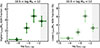 |
Fig. 8. Similar to Fig. 7, but presented in four ΣSFR, 1 kpc bins. |
| In the text | |
|
Fig. 9. Similar to Fig. 7, but for the fraction of higher-L[OIII]/M★ optical AGNs as a function of ΣSFR, 1 kpc among objects with 10.5 < log M★ < 11 (left) and objects with 11 < log M★ < 12 (right). |
| In the text | |
|
Fig. 10. Fraction of lower-L[OIII]/M★ optical AGNs as a function of ΣSFR, 1 kpc, among objects with 10.5 < log M★ < 11 (left) and objects with 11 < log M★ < 12 (right). |
| In the text | |
|
Fig. 11. Top: Mean ΣSFR, Σ★, ΔMS, Dn4000 profiles of higher-LX/M★ X-ray AGNs compared with normal galaxies in the control sample matched according to M★, SFR, and z individually, sampled with a 1 kpc interval in major-axis radius. Error bars represent the standard error of the mean. Bottom: Similar to the top panel, but for lower-LX/M★ X-ray AGNs. |
| In the text | |
|
Fig. 12. Similar to Fig. 11, but for higher-L[OIII]/M★ optical AGNs (top) and lower-L[OIII]/M★ optical AGNs (bottom). |
| In the text | |
|
Fig. 13. Left: Violin plot showing the distribution of differences in ΣSFR between higher-LX/M★ AGNs and matched control galaxies at each radius. Similar to the mean ΣSFR profiles presented in Fig. 11, clear differences in the medians are also observed, especially in the central regions. However, the distributions of Δ log ΣSFR for individual matched pairs remain broad, spanning both positive and negative values. Right: Similar to the left panel, but for lower-LX/M★ AGNs. The Δ log ΣSFR distributions are also broad, while no clear differences in the medians are observed in galaxy central regions (aligning with the lack of significant differences in the mean ΣSFR profiles). |
| In the text | |
|
Fig. 14. Similar to Fig. 13, but for higher-L[OIII]/M★ optical AGNs (left) and lower-L[OIII]/M★ optical AGNs (right). Consistent with the clear differences in the mean ΣSFR profiles presented in Fig. 12, offsets in the median values of the distributions (indicated by short horizontal lines) are observed for both groups in the central regions of galaxies. The overall distributions of Δ log ΣSFR for individual matched pairs are broad, extending significantly into both positive and negative values. |
| In the text | |
|
Fig. 15. SFR surface density profiles estimated from Hα, of X-ray AGNs with lower LX/M★ (log LX/M★ < 30.5) and normal galaxies utilized in Fig. 11. We can see that even the mean ΣSFR estimated from Hα emission from spaxels that are not AGN-dominated is elevated compared to that of non-AGNs in the control galaxy sample, suggesting that a minute level of SF enhancement is likely among the hosts of these very weak AGNs, when we select an SF indicator that is sensitive to very recent SF activity. |
| In the text | |
|
Fig. 16. Left: Mean ΔMS profiles of all the galaxies in the sample grouped according to their M★ and SFR values. Error bars represent the standard error of the mean. Right: Similar to the left panel, but for ΣsSFR profiles. |
| In the text | |
|
Fig. 17. Mean ΣSFR profiles of galaxies in the sample grouped according to their M★ and SFR values. Error bars represent the standard error of the mean. |
| In the text | |
Current usage metrics show cumulative count of Article Views (full-text article views including HTML views, PDF and ePub downloads, according to the available data) and Abstracts Views on Vision4Press platform.
Data correspond to usage on the plateform after 2015. The current usage metrics is available 48-96 hours after online publication and is updated daily on week days.
Initial download of the metrics may take a while.