


| Issue |
A&A
Volume 711, July 2026
|
|
|---|---|---|
| Article Number | A144 | |
| Number of page(s) | 12 | |
| Section | Cosmology (including clusters of galaxies) | |
| DOI | https://doi.org/10.1051/0004-6361/202659201 | |
| Published online | 16 July 2026 | |
ComPACT: Mass-redshift properties of the galaxy cluster catalogue
1
Space Research Institute (IKI) Russian Academy of Sciences, Profsoyuznaya 84/32 Moscow 117997, Russia
2
HSE University, 20 Myasnitskaya St., Moscow 101000, Russia
3
Faculty of Computational Mathematics and Cybernetics of Lomonosov, Moscow State University, Moscow 119234, Russia
★ Corresponding authors: This email address is being protected from spambots. You need JavaScript enabled to view it.
; This email address is being protected from spambots. You need JavaScript enabled to view it.
Received:
29
January
2026
Accepted:
20
May
2026
Abstract
Context. Machine-learning methods are more and more frequently applied to astronomical surveys, offering powerful tools for detecting and studying galaxy clusters.
Aims. We investigate the mass-redshift properties and completeness of the COMPACT galaxy cluster catalogue, constructed using a convolutional neural network (CNN) applied to publicly available, combined ACT+Planck maps.
Methods. The ComPACT catalogue contains 2962 SZ-selected galaxy cluster candidates. We confirmed the clusters by estimating redshifts using literature data and photometric techniques based on DESI Legacy Imaging Surveys. Cluster masses were derived from ACT+Planck and Planck Compton-y maps via SZ scaling relations. The completeness was assessed using simulated cluster injections into real microwave maps.
Results. We confirmed approximately ∼60% of the ComPACT candidates as galaxy clusters. The redshift span covers the range 0.007 < z < 1.7, including approximately 116 new measurements. Masses were obtained for 56% of the sample, covering the range (0.25 − 13.1)×1014 M⊙ and including 158 new mass determinations. We identified five previously unreported massive clusters (M500c > 6 × 10¹⁴ M⊙) at z > 0.7, increasing the known population of such systems by approximately 10%.
Conclusions. The ComPACT catalogue expands the SZ-selected Planck-like cluster population, especially at high redshifts and high masses, demonstrating the effectiveness of deep-learning approaches for cluster detections in microwave data.
Key words: methods: data analysis / techniques: photometric / catalogs / galaxies: clusters: general / submillimeter: galaxies
© The Authors 2026
 Open Access article, published by EDP Sciences, under the terms of the Creative Commons Attribution License (https://creativecommons.org/licenses/by/4.0), which permits unrestricted use, distribution, and reproduction in any medium, provided the original work is properly cited.
This article is published in open access under the Subscribe to Open model. This email address is being protected from spambots. You need JavaScript enabled to view it. to support open access publication.
1. Introduction
Galaxy clusters are the most massive gravitationally bound systems in the Universe and they constitute key probes of cosmology and galaxy evolution. They form at the sites of rare, high-amplitude primordial matter density fluctuations in the early Universe (Sarazin 1988). As the largest virialised structures, galaxy clusters provide valuable laboratories for studying the growth of large-scale structure, cosmic evolution, and the interplay between dark matter, the hot intracluster medium, and cluster galaxies (see, e.g., Allen et al. 2011; Kravtsov & Borgani 2012, for reviews). The total mass of galaxy clusters is dominated by dark matter (approximately 85%), which defines the gravitational potential well that confines the hot, X-ray-emitting intracluster gas.
Photons undergo inverse Compton scattering off the hot electrons in galaxy clusters, resulting in a characteristic distortion of the cosmic microwave background blackbody spectrum known as the thermal Sunyaev–Zeldovich (tSZ) effect (Sunyaev & Zeldovich 1970, 1972). Owing to the redshift independence of the tSZ surface brightness, galaxy clusters can be detected in the microwave band out to the highest redshifts. The first galaxy clusters discovered in a blind survey via their tSZ signature were reported more than a decade ago (Staniszewski et al. 2009). Since then, substantial progress in tSZ-selected cluster studies has been achieved by the South Pole Telescope (SPT; Huang et al. 2020; Bleem 2020; Klein et al. 2024a), the Atacama Cosmology Telescope (ACT; Hilton et al. 2018, 2021; Klein et al. 2024b; Aguena et al. 2026), and the Planck satellite mission (Planck Collaboration XX 2014; Planck Collaboration XXII 2016).
Cluster redshifts are generally determined from the spectroscopy or photometry of their member galaxies (e.g. Bocquet et al. 2019), providing distance estimates that are essential in mapping the large-scale structure and for use in cosmological analyses. Cluster masses, in turn, can be inferred using a variety of techniques that probe different cluster components (see, e.g. Pratt et al. 2019; Miyatake 2025, for a review). A number of X-ray mass proxies have been proposed and are commonly used to determine individual cluster masses (Kravtsov et al. 2006; Pratt et al. 2009; Arnaud et al. 2010; Mantz et al. 2018; Churazov et al. 2015; Pratt et al. 2022; Lyskova et al. 2025; Kruglov et al. 2025, among others). The total SZ flux also correlates tightly with the total cluster mass (e.g., Nagai 2006; Arnaud et al. 2010; Planck Collaboration XX 2014, among many others). Weak gravitational lensing enables a direct probe of the underlying dark matter potential (e.g. McClintock et al. 2019), independently of the cluster dynamical state. Dynamical analysis based on the galaxy velocity dispersions, on par with weak lensing techniques, is considered to provide unbiased cluster mass estimates (e.g. Evrard et al. 2008; Saro et al. 2013; Ferragamo et al. 2021). All these different techniques establish the connection between observed quantities and the underlying halo properties, enabling the use of galaxy clusters as cosmological probes and as environments for studying baryonic processes in dense regions.
Over the past decade, several extensive catalogues of SZ-selected galaxy clusters have been compiled. The full-sky survey conducted by Planck resulted in the PSZ2 catalogue (Planck Collaboration XX 2014), which includes 1,653 SZ-detected objects, 1,334 of which have been confirmed through optical observations (Bahk & Hwang 2024). Atacama Cosmology Telescope (ACT), in its fifth data release (DR5), provided over 4000 optically confirmed SZ clusters across an area of approximately 13 211 deg2 (Hilton et al. 2021). More recently, ACT DR6 reported around 10 000 galaxy clusters (Aguena et al. 2026), significantly surpassing the volume of previous SZ catalogues. The South Pole Telescope (SPT) identified 677 cluster candidates in a 2500 deg2 survey, of which 516 have been confirmed (Bleem et al. 2015). These catalogues are further complemented by more recent datasets from SPTpol (Bleem 2020) and SPT-DEEP (Kornoelje et al. 2025).
To increase the number of galaxy clusters identified in current data, several complementary strategies have been pursued. One approach involves combining microwave observations from multiple instruments, as demonstrated by the joint analysis of Planck and SPT data (PSZSPT; Melin et al. 2021), which revealed several dozen clusters absent from the individual SPT/Planck catalogues. Another method exploits the synergy between different wavebands, for example, by cross-correlating microwave and X-ray observations. Tarrío et al. (2019) combined Planck and ROSAT all-sky survey data to construct the ComPRASS catalogue, which contains nearly 2000 joint X-ray–SZ detections, around one quarter of which were previously unknown. A further avenue involves extending existing cluster-confirmation algorithms. For instance, Klein et al. (2024b,a), Hernández-Lang et al. (2023) applied the multi-component matched filter approach with optical survey data to follow up low signal-to-noise ratio (S/N) SZ detections, enabling the discovery of a large number of lower-mass systems not identified in published catalogues.
Over the past decade, machine learning (ML) techniques have become increasingly prominent in the analysis of tSZ data. These methods enable data-driven inference, allowing signal detection and classification without relying on predefined models or templates (for a review, see Moriwaki et al. 2023). In the context of SZ studies, deep learning approaches have proven particularly effective for signal extraction and component separation. For example, Bonjean (2020) and Meshcheryakov et al. (2022) applied a U-Net convolutional neural network (CNN) to the multifrequency, full-sky Planck maps. Meshcheryakov et al. (2022) network successfully recovered all previously known Planck SZ clusters and identified a large number of new cluster candidates through component separation. Similarly, Lin et al. (2021) trained a CNN on simulated microwave intensity maps and compared its performance to the conventional matched filter (MF) approach. Although both methods recovered high-S/N systems, the CNN was able to identify lower-S/N clusters missed by the MF. Moreover, combining the outputs of both methods improved overall completeness at fixed purity. In the optical domain, Grishin et al. (2023, 2025) developed the YOLO–CL algorithm, an object detection CNN trained on SDSS colour images using redMaPPer clusters as training labels. The model successfully recovered 95–98% of known clusters with comparable purity, illustrating the effectiveness of modern deep learning techniques in identifying cluster-like structures across multiple wavelengths.
In this work, we analyse an SZ galaxy cluster catalogue based on machine learning, presented in Voskresenskaia et al. (2024). The catalogue, referred to as ComPACT, was constructed using a deep learning, CNN-based method, applied to combined ACT+Planck intensity maps. It was built by targeting regions surrounding SZcat sources (Meshcheryakov et al. 2022) with the aim of identifying Planck-like clusters that fall below the detection threshold of the original Planck survey. A key advantage of this deep learning approach over traditional matched-filter techniques, as demonstrated in Voskresenskaia et al. (2024), is its ability to learn complex, non-linear patterns in the data directly, potentially leading to improved sensitivity to lower S/N systems compared to methods that rely on a fixed cluster template (e.g. Lin et al. 2021; Bonjean 2020; Bonjean et al. 2024; Ntampaka et al. 2019).
The primary goals of this paper are two-fold. First, we assess the quality and robustness of the ComPACT catalogue by evaluating its completeness and identifying potential biases using simulations. Second, we investigate the redshifts and masses of its constituent clusters to characterise the population revealed by the DL detection method. Redshifts have been obtained using a combination of photometric techniques and cross-matching with existing spectroscopic and photometric redshift data, while masses are estimated via Y–M scaling relations from SZ observables measured in this work.
This paper is organised as follows. In Section 2, we describe the data sources and external catalogues used in our analysis. Section 3 outlines the methodology for photometric redshift estimation, while Section 4 details the procedures for deriving cluster masses. Section 5 presents the main results, including completeness and empirical purity, as well as a discussion of particularly notable cluster candidates. We conclude with a summary of our findings in Section 6. Masses are reported in terms of M500c if not stated otherwise, where M500c is defined as the mass enclosed within a radius of R500c, at which the average density is 500 times the critical density at the cluster redshift. We assumed a flat lambda cold dark matter (ΛCDM) cosmology with Ωm = 0.3, ΩΛ = 0.7, and H0 = 70 km s−1 Mpc−1 throughout.
2. Data
The ComPACT catalogue spans the ACT survey footprint (∼18 000 deg2) and contains a total of 2,962 SZ-selected cluster candidates, detected using the ACT+Planck intensity maps with a DL model, of which 1 220 have been validated as galaxy clusters in existing catalogues. These candidates are assigned priority I–III reliability classes, with priority I (N = 1720) having an expected purity of ∼84%, as estimated in Voskresenskaia et al. (2024). Below, we summarise the multi-wavelength data sets used for cluster confirmation, redshift estimation, and mass calibration:
-
Optical/infrared imaging (redshift estimates): We used deep optical photometry from (i) the DESI Legacy Imaging Surveys (e.g. DECaLS DR9, Dey et al. 2019), which provide optical g, r, z photometry combined with 3.4 and 4.6 μm photometry from WISE (Wright et al. 2010). These data are crucial for detecting red-sequence galaxies across most of the ACT cluster search regions; and (ii) the Wide-field Infrared Survey Explorer (WISE; Wright et al. 2010; Burenin 2022) provides all-sky mid-infrared photometry in W1 and W2.
-
Compton y-maps (mass estimates): For SZ-based mass estimation, we used the publicly available combined ACT+Planck Compton-y map from NASA/LAMBDA1, which covers roughly one-third of the sky with a resolution of 0.5 arcmin per pixel (Coulton et al. 2024). We also used the Planck full-mission NILC y-map (HEALPix Nside = 2048, 1.72 arcmin per pixel; Chandran et al. 2023). For each cluster in the catalogue, we extracted its SZ signal from the maps to estimate its mass.
-
ACT+Planck intensity maps (completeness characterisation): To assess the completeness of the ComPACT catalogue, we employed the combined ACT DR5+Planck sky intensity maps at 90, 150, and 220 GHz (Naess et al. 2020) available from LAMBDA2, with a resolution of 0.5 arcmin per pixel, covering ∼18 000 deg2.
3. Redshift measurements
Measuring galaxy cluster redshifts is essential for determining their distances, estimating their masses, and enabling their use in astrophysical analyses. We adopt a hierarchical strategy to obtain redshift information uniformly across all priorities. Redshifts are obtained by cross-matching with external catalogues and by combining the zCluster (Hilton et al. 2018, 2021) algorithm with the method of Zaznobin et al. (2023) (hereafter Zaznobin; see Section 3.2 for details).
3.1. Literature redshifts
The ComPACT catalogue is validated through cross-identification with previously known galaxy clusters from SZ, X-ray, and optical surveys (see Table 1). Using a matching radius of 5 arcmin, motivated by the analysis of average radial number density profiles around ComPACT candidates (see Appendix B1 in Voskresenskaia et al. 2024), we identified counterparts for 56% of the sample (1 668 clusters).
Public cluster catalogues cross-matched with ComPACT.
Among these associations, 258 correspond to clusters reported in catalogues published after the release of ComPACT, including ACT DR6, ACT-MCMF, SPT-DEEP, MCXC2 (excluding MCXC), and MaDCoWS II. Redshift information is available in the literature for 1 656 of the matched systems. When a spectroscopic redshift (zspec) is available, we adopt it as the cluster redshift; otherwise, we use the published photometric redshift (zphot).
3.2. Photometric redshift estimation for clusters without literature redshifts
For galaxy clusters without previously reported redshifts, we apply two independent photometric methods: the Zaznobin algorithm and the zCluster method. Both approaches analyse the redshift distribution of galaxies around the cluster centre and identify the most significant overdensity corresponding to the cluster redshift. Our selection scheme is as follows: (i) if a redshift from the Zaznobin method is available, we adopt it; and (ii) otherwise, we use the zCluster estimate.
3.2.1. Zaznobin method
The algorithm used in this work is a modified version of the method presented by Zaznobin et al. (2023)3. In the original approach, cluster redshifts were estimated using X-ray data from the eROSITA survey, infrared data from WISE survey in the W1 band (Wright et al. 2010), and galaxy photometric redshifts from Zou et al. (2022), derived from the DESI Legacy Imaging Surveys DR9 (Dey et al. 2019).
Since X-ray data were not used in the present analysis, the algorithm was adapted to the available data sets. Instead of X-ray information, we used the positions and mass estimates of the SZ sources. When no mass estimate was available, a fiducial mass of M500c = 1014 M⊙ was assumed. This fiducial mass was validated on a spectroscopic subsample. The lower thresholds increased sample size, but degraded the Area Under the Receiver Operating Characteristic Curve (AUC) score of redshift estimates; whereas the adopted value tends to maximise completeness, while maintaining high AUC and minimising redshift scatter.
As in the original work, the method consists of two stages.
3.2.1.1. Stage 1: Preliminary redshift.
An optical association of galaxies with SZ sources is performed to obtain a preliminary redshift estimate, zprel. At this stage, galaxies are selected from the catalogue of Zou et al. (2022) within a predefined spatial region. The distribution of their infrared luminosities is constructed following the procedure described in Zaznobin et al. (2023). The main difference with respect to the original method is that the galaxy selection is centred on the SZ source coordinates (RA, Dec) and the spatial selection criteria are modified. Galaxies are selected within an angular radius of 534 arcsec from the centre of the SZ source, corresponding to the angular size of R500c for a galaxy cluster with a mass of M500c = 3 × 10¹⁴ M⊙ at z = 0.1. In addition, a cut on the projected physical distance of 814 kpc is applied, corresponding to R500c for a cluster of the same mass at z = 0.6. As in Zaznobin et al. (2023), the preliminary redshift estimate is defined as the redshift corresponding to the maximum of the infrared luminosity distribution.
3.2.1.2. Stage 2: Refined redshift.
Cluster redshift is refined using the same methodology as in Zaznobin et al. (2023). Galaxies with photometric redshift estimates photo_z and corresponding redshift uncertainties phot_zerr from the catalogue of Zou et al. (2022) are selected according to the following criteria:
-
projected distance r < R500c;
-
relative photometric redshift uncertainty phot_zerr/(1 + photo_z) < 2%;
zprel − 0.06(1+zprel) < photo_z<zprel + 0.06(1+zprel).
For the selected galaxies, a refined cluster redshift is computed as the inverse-variance-weighted mean of their photometric redshifts, with weights given by the inverse squared photometric redshift uncertainties. The standard deviation of the distribution is computed simultaneously. An iterative 2σ-clipping procedure is then applied: at each iteration, galaxies deviating by more than 2σ from the mean are removed. The procedure was repeated until no further galaxies are rejected. The final weighted mean redshift is adopted as the refined cluster redshift.
In the original study, the reliability of the cluster identification was quantified using a parameter defined as the product of two factors, p1 and p2 (Zaznobin et al. 2023). In the present work, instead of applying a threshold to their product, independent thresholds were imposed on each factor. The parameters p1 and p2 were computed using a sample of 104 random positions. Since the procedures used to estimate both preliminary and refined redshifts are modified, the reliability parameters are recomputed for the random sample.
Only objects satisfying p1 > 0.978 and p2 > 0.8 are included in the final analysis. These thresholds correspond to a false-positive rate of approximately 5%. After applying this selection, we obtain 47 new photometric redshift estimates.
3.2.2. zCluster method
zCluster4 is a photometric redshift estimation algorithm for galaxy clusters, originally presented by Hilton et al. (2018, 2021). The method estimates cluster redshifts using broadband photometry, assuming prior knowledge of the cluster position on the sky. In this work, we apply zCluster to photometric data from the DECaLS DR9 survey (Dey et al. 2019).
For each galaxy located in the vicinity of the cluster position, an individual photometric redshift probability distribution, p(z), is computed using template fitting. These individual probability distributions are then combined into a single cluster redshift probability distribution through a weighted summation. The weights account for the projected distance of each galaxy from the cluster centre, reflecting the expected radial distribution of galaxies in a cluster, as well as the quality of the photometric measurements. Consequently, galaxies which are closer to the cluster centre and with more reliable photometric redshift estimates contribute more strongly to the combined probability distribution.
To suppress noise fluctuations and enhance coherent redshift features, the combined probability distribution is smoothed by integrating the individual p(z) distributions over a redshift window, yielding the quantity nΔz(z). The photometric redshift of the cluster is then defined as the redshift corresponding to the maximum of this smoothed distribution.
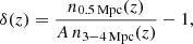
To quantify the optical overdensity associated with the cluster and to assess the reliability of the redshift estimate, zCluster defines a contrast parameter,
 (1)
(1)
where z is the estimated cluster redshift, n0.5 Mpc(z) is the number of galaxies within a projected radius of 0.5 Mpc from the cluster centre, and n3–4 Mpc(z) is the background galaxy number density estimated within an annulus spanning projected radii of 3–4 Mpc. The factor A accounts for the difference in area between the inner aperture and the background annulus.
The selection of spectral templates used to compute the galaxy photometric redshift probability distributions is calibrated using a randomly selected subsample of 114 ACT DR5 clusters from the ComPACT catalogue. We investigated the impact of different template sets, including the COSMOS galaxy and active galactic nucleus templates (Ilbert et al. 2009; Salvato et al. 2011) and CWW templates (Coleman et al. 1980)). Based on this analysis, we adopted a combination of two galaxy templates (Sb_A_0, Sb_template_norm) for the zClusterδ measurement and redshift determination at z > 0.2, as this choice yields the best performance in terms of photo-z dispersion and the fraction of catastrophic outliers for the ComPACT clusters with available spectroscopic redshifts.
Following the approach adopted for the main redshift estimation algorithm, the reliability of the zCluster redshift measurements was assessed using the distribution of δ measured at random positions (see Appendix B). Based on this analysis, we adopted a threshold corresponding to a false-positive rate of 5%, which translates into a requirement of δ ≥ 3. Only objects satisfying this criterion were included in the final sample. After applying this selection, we obtained 69 new photometric redshift measurements.
3.3. Comparison of photometric methods
Figure 1 compares the cumulative redshift distributions and photometric redshift performance for clusters with available spectroscopy.
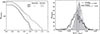 |
Fig. 1. Comparison of cluster redshift estimates obtained with the Zaznobin method and with zCluster. Left: Cumulative redshift distribution of cluster candidates obtained with the Zaznobin method and with zCluster. The Zaznobin method is especially effective for low-redshift systems (z < 0.2), whereas zCluster is able to recover clusters out to higher redshifts (z ≳ 0.8). Right: Distribution of the photometric redshift error, δz/(1 + zspec), for clusters with spectroscopic redshifts. |
The Zaznobin method achieves μ = 0.0030, σ = 0.0068, and an outlier fraction |δz|/(1 + z) > 20% of 0.011. The zCluster method yields μ = −0.0019, σ = 0.0115, and an outlier fraction of 0.007. Zaznobin provides higher precision at low redshift (z < 0.8), while zCluster extends to higher redshifts (z ≳ 0.8) with a slightly lower catastrophic outlier fraction.
When compared directly on the spectroscopic subsample, the two methods demonstrate an excellent agreement: the normalised median offset is median[Δz/(1 + z)] = −0.0051, with a robust scatter of σNMAD = 0.0111. This consistency between independent methodologies supports the robustness of our cluster redshift estimates.
3.4. Final redshift sample and completeness
The resulting sample of 1771 galaxy clusters with measured redshifts (spectroscopic or photometric) has a mean redshift of ⟨z⟩ = 0.43, comparable to other SZ-selected samples, and covers the range 0.007 < z < 1.795. For the ComPACT catalogue, the total number of clusters with spectroscopic redshifts is 1 027 clusters (∼34%), while the photometric redshifts are available for an additional 628 (21.2%) clusters. Our photometric analysis provides 116 new redshift measurements. The redshift completeness depends on the catalogue priority: the priority I subsample reaches 76% completeness, compared to 44.6% for priority II and 33.5% for priority III. The overall redshift completeness of the full ComPACT catalogue is 60%.
4. Mass estimation
Cluster masses are derived using SZ measurements from the ACT+Planck and Planck Compton-y maps, complemented by values available in the literature. To derive mass estimates for clusters, we used the following approaches:
-
(1)
We cross-matched our candidates with previously published catalogues (see Table 1) and extracted the available SZ, X-ray, and optically-derived mass estimates. As these estimates are affected by different systematics and calibration biases, we included the mSource column to specify the origin of each mass estimate. Selecting cluster candidates based on mSource allowed us to construct subsamples with masses defined consistently across the sample.
-
(2)
For unmatched objects, we detected these cluster candidates in the ACT+Planck y-map by computing the S/N. Prior to the signal extraction, the ACT+Planck y-map, originally in plate-carée projection with 0.5 arcmin per pixel, was reprojected to the HEALPix format with Nside = 8192 to preserve the native pixel scale. To calculate the signal, we defined a circular region with a radius of r = 1.6 arcmin and computed the maximum tSZ signal within this aperture. To estimate the noise, we followed Isopi et al. (2025) and used a background annulus around each candidate. The annulus had an inner radius of R1 = 30 × r, measured from the candidate centre, and an outer radius of R2 = R1 + 30′. Within this annulus, we measured the maximum tSZ signal in 1 000 randomly placed circular apertures (each 1.6 arcmin in radius) and compute the mean (ybkg) and standard deviation (σbkg) of these values. The S/N is given by
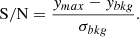 (2)
(2)Clusters were selected with S/N5 > 2 corresponding to 5% of false detections (for details, see App. B). To estimate the mass, we computed the ’cylindrical’ integrated Ycyl parameter within an aperture of R = 10′ to ensure consistency with Planck, where the map resolution (FWHM) is approximately 10 arcmin. The measured Ycyl was scaled by a factor a to match the Planck measurements. We derive a = 0.8 by matching our Y-values to Planck Y-measurements for a calibration set of PSZ2 clusters processed with identical apertures. Then, Ycyl is then converted to a ‘spherical’ Y500 following the procedure described in Melin et al. (2011), which assumes a gNFW pressure profile. Finally, the mass, M500c, was derived using the scaling relation from Planck Collaboration XX (2014) (for details, see App. C).
-
(3)
For regions not covered by the ACT+Planck y-map, we use the Planck y-map. Cluster detection is performed using the same background-annulus methodology as for the ACT+Planck y-map. The aperture radius of R = 1.6′ was selected by maximising the recovery fraction of PSZ2 clusters (yielding a completeness of 89%) at a fixed false detection rate of 5%, corresponding to a detection threshold of S/N > 1.7. This angular scale also closely matches the native HEALPix pixel size of the Planck NILC map (∼1.72′ for Nside = 2048). The mass is then estimated from the measured Y-values using the same scaling relation as above.
We obtained mass measurements for 56% of the full catalogue and for 72.9% of the priority I subsample. The average mass of the ComPACT sample with available mass estimates is ⟨M500c⟩ = 4 × 10¹⁴ M⊙, with values ranging from 0.25 × 10¹⁴ to 13.1 × 10¹⁴ M⊙. In total, we have provided 158 new mass measurements: 114 derived from ACT+Planck and 44 from Planck y-maps.
5. Results
5.1. Completeness
The completeness of SZ-catalogues is typically estimated by injecting the UPP model clusters into maps and measuring the recovery rates (Hasselfield et al. 2013; Planck Collaboration XXVII 2016). This follows, for example, the implementation employed in the ACT DR5 analyses (Hilton et al. 2018). We assessed the ComPACT catalogue completeness in a similar way by injecting synthetic clusters are injected into the real ACT+Planck maps and passing them through the deep-learning detection pipeline (see Appendix D for details). The left panel of Figure 2 shows the completeness in the (M500c, z) plane for detections with pmax > 0.8 and S > 20 (see Fig. 5 in Voskresenskaia et al. (2024)) without selection in SZcat directions. Here, pmax denotes the maximum classification probability assigned by the neural network to a detected object, while S is the area of the detection in pixel units; both quantities characterise objects after a classification. These selection thresholds are applied after the classification stage and the analysis is restricted to the ACT DR5 footprint (13 211 deg2).
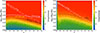 |
Fig. 2. Estimated completeness of the DL based cluster catalogue (without Planck SZcat selection) in the (M500c, z) plane. The black dashed line corresponds to detection thresholds of pmax > 0.8 and S > 20. The white dash-dotted line represents the average mass evolution of a 2 × 10¹⁵ M⊙ cluster over redshift (from Fakhouri et al. 2010). Left panel: Within the ACT DR5 footprint (13 211 deg2). The black dashed contour shows the 90% completeness of the catalogue, while the solid yellow line marks the same level for the ACT DR5 S/N > 3 catalogue at matched purity. The ComPACT achieves higher completeness than ACT DR5S/N > 3 at fixed purity, especially for massive clusters at high redshift, while both catalogues perform comparably at low z. Right panel: Outside the ACT DR5 footprint (∼3000 deg2). Catalogue retains high completeness for massive clusters across the redshift range, demonstrating its potential to identify new systems beyond existing survey coverage. |
To enable a direct comparison with the cumulative completeness estimate reported in Voskresenskaia et al. (2024), we also computed the integrated completeness from our simulations for clusters with M500c > 1014 M⊙ across the full redshift range. We obtain a cumulative completeness of 77%. This value differs from the ≈70% reported in Voskresenskaia et al. (2024) because our simulation-based estimate does not include the selection by SZcat directions applied to the ComPACT catalogue; consequently, the 77% value should be interpreted as an upper limit on the ComPACT completeness.
For a fair comparison with ACT DR5, we matched the catalogues at equal purity. Using the NEMO6 package, we obtained the ACT DR5 S/N > 3 sample (yellow 90% contour in the left panel of Fig. 2), corresponding to a purity of ∼20%, consistent with the full catalogue prior to SZcat-based selections. We note here that the mass scales of the ComPACT and ACT DR5 catalogues are aligned by construction, since both analyses use the same input M500c distribution of synthetic clusters. At low redshift, both catalogues exhibit similar completeness, but the DL approach recovers more massive systems at higher redshifts. Overall, the ComPACT catalogue achieves higher completeness than ACT DR5 at fixed purity. This behaviour indicates that the deep-learning approach has improved sensitivity to lower S/N systems compared to traditional matched-filter methods, particularly at high redshift.
The dash-dotted curve shown in the left panel of Fig. 2 represents the median mass accretion history of dark matter halos from Fakhouri et al. (2010). It is included as a reference to illustrate the expected evolutionary relation between cluster mass and redshift and to guide the interpretation of the completeness limits in the (M500c, z) plane and to distinguish the population of the most massive clusters.
The same analysis is repeated for the ComPACT survey region, excluding ACT DR5 field to avoid overlap (∼3000 deg2). Outside the footprint of ACT DR5 catalogue (see right panel of Fig. 2), our catalogue demonstrates higher completeness for massive galaxy clusters across the entire redshift range. This indicates that in these regions, the most massive cluster candidates may be discovered, and this prediction is borne out by our optical/NIR follow-up observations (Sec. 5.3).
5.2. Confirmation of clusters
Cluster candidates are considered as confirmed clusters if they satisfy at least one of the following criteria:
-
They display a cross-match with the galaxy cluster catalogues listed in Table 1. In total, 1 668 clusters have such counterparts.
-
They have been identified by the zCluster algorithm with an optical contrast of δ > 3 (69 objects) or by their Zaznobin score, whereby p1 > 0.978 and p2 > 0.8 corresponds to 5% false-positive rate (47 objects), as detailed in Section 3).
Table 2 summarises the number and fraction of cluster candidates, together with the corresponding purity, classified as confirmed, with redshift estimates, with mass estimates, or newly identified with redshift and mass estimates, both inside and outside the ACT DR5 and DESI Legacy Imaging Surveys (LIS; DeCALS DR9) footprints. The fraction of confirmed clusters is significantly higher inside the ACT DR5 footprint (63.2%) than outside (38.2%). A similar trend is observed for the DESI LIS footprint, where 62.5% of candidates inside the footprint are confirmed, compared to 49.2% outside. This decrease by approximately 10% in the confirmation rate outside the survey footprints is primarily driven by fewer photometric data from DESI LIS. As a consequence, we expect that future redshift follow-up efforts may increase the confirmed fraction outside the ACT DR5 footprint by up to ∼10%.
Number and percentage of candidates in different regions.
Table 3 provides a summary of the number and fraction of sources in the full catalogue and in the priority I subsample. As expected, the priority I subset exhibits the highest reliability: 76% of its candidates are confirmed, compared to 60.2% in the full sample. Redshift estimates are obtained for 59.8% of all candidates. The Zaznobin method yields larger number of redshift determinations, exceeding those derived with zCluster. Mass estimates are available for 56% of the full catalogue. Using the ACT+Planck Compton-y maps, masses can be derived for 48.6% of the candidates, while the Planck-only y maps allow mass measurements for 46.5%. We also identified 116 previously unreported systems, among which 72 have both redshift and mass estimates. The priority I subsample contributes 26 such new clusters.
Number and percentage of candidates that are classified in the three different classes in full catalogue and in priority I.
5.3. Mass-redshift behaviour
Figure 3 shows the mass–redshift distribution for ComPACT clusters. For comparison with existing surveys, we overlay contours from the ACT DR6 catalogue (purple), the PSZ2 catalogue (blue) and SPT-DEEP (orange). Known clusters from external catalogues included in ComPACT (see Table 1) are shown as dots, while stars denote objects with newly determined redshifts. Colours indicate the source of the mass estimate: grey for masses from literature, green for M500c from the Planck y-map, and magenta for masses from the ACT+Planck y-map.
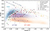 |
Fig. 3. Comparison of the ComPACT cluster sample in the mass–redshift plane. The distribution of ComPACT clusters is shown alongside those from ACT DR6 (purple contours), PSZ2 (blue contours), and SPT-DEEP (orange contours). The dashed lines trace the mass evolution of 2 and 3 × 10¹⁵ M⊙ clusters at z = 0 for a fixed cosmology (Fakhouri et al. 2010). Circles indicate clusters with redshifts from the literature (Table 1), while stars denote clusters with newly determined redshifts. Colours distinguish cluster categories: grey points mark ComPACT clusters with literature mass measurements, green points indicate new mass estimates from Planck y-maps, and magenta points show new mass estimates from ACT+Planck y-maps. Clusters with newly determined redshifts and masses are highlighted in green. Orange points above the 2 × 10¹⁵ M⊙ line represent clusters from the catalogues listed in Table 1 that are not included in ComPACT. |
As made evident from the figure, a significant fraction of new ComPACT clusters lies below the PSZ2 distribution and above the ACT DR5 sample, especially at high redshifts (z > 0.8). In this region, many clusters are characterised by newly obtained estimates for both redshift and mass.
5.4. Performance of massive clusters
To assess the contribution of ComPACT at the high-mass end, we applied a mass threshold of 2 × 10¹⁵ M⊙ to all clusters at z > 0.8 in known X-ray and SZ catalogues. In Figure 3, orange dots mark all such massive clusters from catalogues listed in Table 1. Under this cut, ComPACT recovers approximately 30% of these systems, with about 10% being previously unidentified clusters.
We highlight several of the most massive ComPACT systems, identified through zCluster detections, SZ measurements, catalogue cross-matching (e.g., SIMBAD), and visual inspections of optical and IR data. The catalogue includes the well-known Bullet Cluster (ComPACT_G266.020−21.244) and El Gordo (ComPACT_G297.972−67.759), along with newly identified high-mass systems.
In Table 4, we present 14 massive cluster candidates that are detected by the zCluster or Zaznobin algorithm, including 11 newly identified objects as well as previously known clusters (see the notes column). Optical images of the clusters are shown in Figure 4. As noted by Burenin et al. (2021), not all massive Planck clusters exceed the detection threshold of the PSZ2 catalogue. This can be explained in the context of selection effects in SZ surveys, such as template mismatch and reduced sensitivity to systems with large angular extent or lower SZ signal (e.g., Lin et al. (2021)). Several such clusters are included in Table 4.
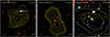 |
Fig. 4. Most massive clusters that are detected by zCluster or Zaznobin algorithms on z = 0.2, 0.69 and 1.2. Each panel shows an optical RGB image from the DESI Legacy Imaging Surveys with overlaid SZ–detection contours. For y-maps, contour levels correspond to μ + σ × {3, 4…}, where μ and σ are estimated locally within an annulus around each cluster, as described in Sect. 4. Contour labels indicate the corresponding significance level in units of σ. |
Sample of massive galaxy clusters detected by the zCluster or Zaznobin algorithms.
6. Conclusions
We present new mass and redshift measurements for the DL based ComPACT galaxy cluster catalogue. This catalogue expands the SZ cluster population by identifying previously unknown systems. The main results are summarised below:
-
By simulating clusters in ACT+Planck maps, we assessed the catalogue completeness across the “mass–redshift” plane. At fixed purity, we find the catalogue achieves higher completeness than ACT DR5S/N > 3 catalogue, particularly improving the recovery of massive high-redshift clusters.
-
The catalogue contains 2962 SZ sources. Cross-matching with existing SZ, X-ray, and optical/IR cluster catalogues yields 1,668 associations. Using DESI LIS surveys photometry, we were able to optically confirm 116 new clusters.
-
Redshifts were obtained for 1771 clusters (60% of the sample), including 116 new measurements. Masses were estimated for 1,659 objects (56%), with 158 new determinations. The median mass is M500c ∼ 4 × 10¹⁴ M⊙, with a median z ∼ 0.43.
Finally, we found five massive (M500c ≳ 6 × 10¹⁴ M⊙) and distant (z > 0.7) clusters. Overall, the ComPACT catalogue, built on the basis of a neural network approach, is a valuable resource for future studies of galaxy clusters in combination with AI.
Data availability
The ComPACT catalogue is publicly available at https://github.com/astromining/ComPACT and will be accessible via the VizieR service. The full machine-readable version of the catalogue is available at the CDS via https://cdsarc.cds.unistra.fr/viz-bin/cat/J/A+A/711/A144.
Acknowledgments
This work was supported by the Russian Science Foundation (Project 𝒩 25-22-00470). We acknowledge the publicly available software packages that were used throughout this work: NumPy (Oliphant 2006; Van Der Walt et al. 2011; Harris 2020), pandas (The pandas development team 2023; Wes McKinney 2010), Matplotlib (Hunter 2007), Astropy (Robitaille 2013; Astropy Collaboration 2018, 2022), pixell https://github.com/simonsobs/pixell, Core Cosmology Library (Chisari et al. 2019), HEALPix package (Górski et al. 2005). We acknowledge the use of the Legacy Archive for Microwave Background Data Analysis (LAMBDA), part of the High Energy Astrophysics Science Archive Center (HEASARC). HEASARC/LAMBDA is a service of the Astrophysics Science Division at the NASA Goddard Space Flight Center. This research is based on observations obtained with Planck (http://www.esa.int/Planck), an ESA science mission with instruments and contributions directly funded by ESA Member States, NASA, and Canada. This research has made use of the SIMBAD database, operated at CDS, Strasbourg, France.
References
- Abdullah, M. H., Wilson, G., Klypin, A., et al. 2020, ApJS, 246, 2 [Google Scholar]
- Aguado-Barahona, A., Barrena, R., Streblyanska, A., et al. 2019, A&A, 631, A148 [NASA ADS] [CrossRef] [EDP Sciences] [Google Scholar]
- Aguena, M., Aiola, S., Allam, S., et al. 2026, Open J. Astrophys., 9, 55863 [Google Scholar]
- Allen, S. W., Evrard, A. E., & Mantz, A. B. 2011, ARA&A, 49, 409 [Google Scholar]
- Arnaud, M., Pratt, G. W., Piffaretti, R., et al. 2010, A&A, 517, A92 [CrossRef] [EDP Sciences] [Google Scholar]
- Astropy Collaboration (Price-Whelan, A. M., et al.) 2018, AJ, 156, 123 [Google Scholar]
- Astropy Collaboration (Price-Whelan, A. M., et al.) 2022, ApJ, 935, 167 [NASA ADS] [CrossRef] [Google Scholar]
- Bahk, H., & Hwang, H. S. 2024, ApJS, 272, 7 [Google Scholar]
- Barrena, R., Streblyanska, A., Ferragamo, A., et al. 2018, A&A, 616, A42 [NASA ADS] [CrossRef] [EDP Sciences] [Google Scholar]
- Bleem, L. E., et al. 2020, ApJS, 247, 25 [CrossRef] [Google Scholar]
- Bleem, L. E., Stalder, B., de Haan, T., et al. 2015, ApJS, 216, 27 [Google Scholar]
- Bocquet, S., Dietrich, J. P., Schrabback, T., et al. 2019, ApJ, 878, 55 [Google Scholar]
- Bonjean, V. 2020, A&A, 634, A81 [NASA ADS] [CrossRef] [EDP Sciences] [Google Scholar]
- Bonjean, V., Tanimura, H., Aghanim, N., Bonnaire, T., & Douspis, M. 2024, A&A, 686, A91 [NASA ADS] [CrossRef] [EDP Sciences] [Google Scholar]
- Burenin, R. A. 2022, Astron. Lett., 48, 153 [Google Scholar]
- Burenin, R. A., Bikmaev, I. F., Gilfanov, M. R., et al. 2021, Astron. Lett., 47, 443 [Google Scholar]
- Chandran, J., Remazeilles, M., & Barreiro, R. B. 2023, MNRAS, 526, 5682 [CrossRef] [Google Scholar]
- Chisari, N. E., Alonso, D., Krause, E., et al. 2019, ApJS, 242, 2 [Google Scholar]
- Churazov, E., Vikhlinin, A., & Sunyaev, R. 2015, MNRAS, 450, 1984 [CrossRef] [Google Scholar]
- Coleman, G. D., Wu, C. C., & Weedman, D. W. 1980, ApJS, 43, 393 [CrossRef] [Google Scholar]
- Coulton, W., Madhavacheril, M. S., Duivenvoorden, A. J., et al. 2024, Phys. Rev. D, 109, 063530 [NASA ADS] [CrossRef] [Google Scholar]
- Dey, A., Schlegel, D. J., Lang, D., et al. 2019, AJ, 157, 168 [Google Scholar]
- Di Francesco, J., Johnstone, D., Kirk, H., MacKenzie, T., & Ledwosinska, E. 2008, ApJS, 175, 277 [Google Scholar]
- Evrard, A. E., Bialek, J., Busha, M., et al. 2008, ApJ, 672, 122 [Google Scholar]
- Fakhouri, O., Ma, C.-P., & Boylan-Kolchin, M. 2010, MNRAS, 406, 2267 [Google Scholar]
- Ferragamo, A., Barrena, R., Rubiño-Martín, J. A., et al. 2021, A&A, 655, A115 [NASA ADS] [CrossRef] [EDP Sciences] [Google Scholar]
- Finoguenov, A., Rykoff, E., Clerc, N., et al. 2020, A&A, 638, A114 [NASA ADS] [CrossRef] [EDP Sciences] [Google Scholar]
- Górski, K. M., Hivon, E., Banday, A. J., et al. 2005, ApJ, 622, 759 [Google Scholar]
- Grishin, K., Mei, S., & Ilić, S. 2023, A&A, 677, A101 [NASA ADS] [CrossRef] [EDP Sciences] [Google Scholar]
- Grishin, K., Mei, S., Ilic, S., et al. 2025, A&A, 695, A246 [NASA ADS] [CrossRef] [EDP Sciences] [Google Scholar]
- Harris, C. R., Jarrod Millman, K., van der Walt, S. J., et al. 2020, Nature, 585, 357 [NASA ADS] [CrossRef] [Google Scholar]
- Hasselfield, M., Moodley, K., Bond, J. R., et al. 2013, ApJS, 209, 17 [NASA ADS] [CrossRef] [Google Scholar]
- Hernández-Lang, D., Klein, M., Mohr, J. J., et al. 2023, MNRAS, 525, 24 [CrossRef] [Google Scholar]
- Hilton, M., Hasselfield, M., Sifón, C., et al. 2018, ApJS, 235, 20 [Google Scholar]
- Hilton, M., Sifón, C., Naess, S., et al. 2021, ApJS, 253, 3 [Google Scholar]
- Huang, N., Bleem, L. E., Stalder, B., et al. 2020, AJ, 159, 110 [Google Scholar]
- Huang, X., Storfer, C., Gu, A., et al. 2021, ApJ, 909, 27 [NASA ADS] [CrossRef] [Google Scholar]
- Hunter, J. D. 2007, Comput. Sci. Eng., 9, 90 [NASA ADS] [CrossRef] [Google Scholar]
- Ilbert, O., Capak, P., Salvato, M., et al. 2009, ApJ, 690, 1236 [NASA ADS] [CrossRef] [Google Scholar]
- Isopi, G., Capalbo, V., Hincks, A. D., et al. 2025, JCAP, 2025, 078 [Google Scholar]
- Klein, M., Grandis, S., Mohr, J. J., et al. 2019, MNRAS, 488, 739 [Google Scholar]
- Klein, M., Hernández-Lang, D., Mohr, J. J., Bocquet, S., & Singh, A. 2023, MNRAS, 526, 3757 [NASA ADS] [CrossRef] [Google Scholar]
- Klein, M., Mohr, J. J., Bocquet, S., et al. 2024a, MNRAS, 531, 3973 [NASA ADS] [CrossRef] [Google Scholar]
- Klein, M., Mohr, J. J., & Davies, C. T. 2024b, A&A, 690, A322 [NASA ADS] [CrossRef] [EDP Sciences] [Google Scholar]
- Kornoelje, K., Bleem, L. E., Rykoff, E. S., et al. 2025, ApJ, submitted, [arXiv:2503.17271] [Google Scholar]
- Kravtsov, A. V., & Borgani, S. 2012, ARA&A, 50, 353 [Google Scholar]
- Kravtsov, A. V., Vikhlinin, A., & Nagai, D. 2006, ApJ, 650, 128 [Google Scholar]
- Kruglov, A., Khabibullin, I., Lyskova, N., Dolag, K., & Biffi, V. 2025, JCAP, 2025, 007 [Google Scholar]
- Lin, Z., Huang, N., Avestruz, C., et al. 2021, MNRAS, 507, 4149 [NASA ADS] [CrossRef] [Google Scholar]
- Lyskova, N., Churazov, E., Khabibullin, I. I., et al. 2025, A&A, 702, A175 [NASA ADS] [CrossRef] [EDP Sciences] [Google Scholar]
- Mantz, A. B., Allen, S. W., Morris, R. G., & von der Linden, A. 2018, MNRAS, 473, 3072 [NASA ADS] [CrossRef] [Google Scholar]
- McClintock, T., Varga, T. N., Gruen, D., et al. 2019, MNRAS, 482, 1352 [Google Scholar]
- Mehrtens, N., Romer, A. K., Hilton, M., et al. 2012, MNRAS, 423, 1024 [NASA ADS] [CrossRef] [Google Scholar]
- Melin, J. B., Bartlett, J. G., Delabrouille, J., et al. 2011, A&A, 525, A139 [NASA ADS] [CrossRef] [EDP Sciences] [Google Scholar]
- Melin, J. B., Bartlett, J. G., Tarrío, P., & Pratt, G. W. 2021, A&A, 647, A106 [NASA ADS] [CrossRef] [EDP Sciences] [Google Scholar]
- Meshcheryakov, A. V., Nemeshaeva, A., Burenin, R. A., Gilfanov, M. R., & Sunyaev, R. A. 2022, Astron. Lett., 48, 479 [Google Scholar]
- Miyatake, H. 2025, arXiv e-prints [arXiv:2505.07697] [Google Scholar]
- Moriwaki, K., Nishimichi, T., & Yoshida, N. 2023, Rep. Prog. Phys., 86, 076901 [NASA ADS] [CrossRef] [Google Scholar]
- Naess, S., Aiola, S., Austermann, J. E., et al. 2020, JCAP, 2020, 046 [Google Scholar]
- Nagai, D. 2006, ApJ, 650, 538 [Google Scholar]
- Nagai, D., Kravtsov, A. V., & Vikhlinin, A. 2007, in Heating versus Cooling in Galaxies and Clusters of Galaxies, eds. H. Böhringer, G. W. Pratt, A. Finoguenov, & P. Schuecker, 358 [Google Scholar]
- Ntampaka, M., ZuHone, J., Eisenstein, D., et al. 2019, ApJ, 876, 82 [NASA ADS] [CrossRef] [Google Scholar]
- Oliphant, T. 2006, Guide to NumPy [Google Scholar]
- Planck Collaboration XX. 2014, A&A, 571, A20 [NASA ADS] [CrossRef] [EDP Sciences] [Google Scholar]
- Planck Collaboration XXXII. 2015, A&A, 581, A14 [NASA ADS] [CrossRef] [EDP Sciences] [Google Scholar]
- Planck Collaboration XXII. 2016, A&A, 594, A22 [NASA ADS] [CrossRef] [EDP Sciences] [Google Scholar]
- Planck Collaboration XXVII. 2016, A&A, 594, A27 [NASA ADS] [CrossRef] [EDP Sciences] [Google Scholar]
- Pratt, G. W., Croston, J. H., Arnaud, M., & Böhringer, H. 2009, A&A, 498, 361 [NASA ADS] [CrossRef] [EDP Sciences] [Google Scholar]
- Pratt, G. W., Arnaud, M., Biviano, A., et al. 2019, Space Sci. Rev., 215, 25 [Google Scholar]
- Pratt, G. W., Arnaud, M., Maughan, B. J., & Melin, J. B. 2022, A&A, 665, A24 [NASA ADS] [CrossRef] [EDP Sciences] [Google Scholar]
- Rykoff, E. S., Rozo, E., Hollowood, D., et al. 2016, ApJS, 224, 1 [NASA ADS] [CrossRef] [Google Scholar]
- Sadibekova, T., Arnaud, M., Pratt, G. W., Tarrío, P., & Melin, J. B. 2024, A&A, 688, A187 [NASA ADS] [CrossRef] [EDP Sciences] [Google Scholar]
- Salvato, M., Ilbert, O., Hasinger, G., et al. 2011, ApJ, 742, 61 [Google Scholar]
- Sarazin, C. L. 1988, X-ray Emission from Clusters of Galaxies (Cambridge: Cambridge University Press) [Google Scholar]
- Saro, A., Mohr, J. J., Bazin, G., & Dolag, K. 2013, ApJ, 772, 47 [NASA ADS] [CrossRef] [Google Scholar]
- Stanford, S. A., Gonzalez, A. H., Brodwin, M., et al. 2014, ApJS, 213, 25 [CrossRef] [Google Scholar]
- Staniszewski, Z., Ade, P. A. R., Aird, K. A., et al. 2009, ApJ, 701, 32 [CrossRef] [Google Scholar]
- Sunyaev, R. A., & Zeldovich, Y. B. 1970, Ap&SS, 7, 3 [NASA ADS] [Google Scholar]
- Sunyaev, R. A., & Zeldovich, Y. B. 1972, Comm. Astrophys. Space Phys., 4, 173 [Google Scholar]
- Tarrío, P., Melin, J. B., & Arnaud, M. 2019, A&A, 626, A7 [NASA ADS] [CrossRef] [EDP Sciences] [Google Scholar]
- The Astropy Collaboration (Robitaille, T. P., et al.) 2013, A&A, 558, A33 [NASA ADS] [CrossRef] [EDP Sciences] [Google Scholar]
- The pandas development team 2023, pandas-dev/pandas: Pandas (Zenodo) [Google Scholar]
- Thongkham, K., Gonzalez, A. H., Brodwin, M., et al. 2024, ApJ, 967, 123 [NASA ADS] [Google Scholar]
- Van Der Walt, S., Colbert, S. C., & Varoquaux, G. 2011, Comput. Sci. Eng., 13, 22 [Google Scholar]
- Voskresenskaia, S., Meshcheryakov, A., & Lyskova, N. 2024, MNRAS, 531, 1998 [Google Scholar]
- Wen, Z. L., & Han, J. L. 2018, MNRAS, 481, 4158 [CrossRef] [Google Scholar]
- Wes McKinney, 2010, in Proceedings of the 9th Python in Science Conference, eds. S. van der Walt, & J. Millman, 56 [Google Scholar]
- Wright, E. L., Eisenhardt, P. R. M., Mainzer, A. K., et al. 2010, AJ, 140, 1868 [Google Scholar]
- Zaznobin, I. A., Burenin, R. A., Meshcheryakov, A. V., et al. 2023, Astron. Lett., 49, 431 [Google Scholar]
- Zou, H., Sui, J., Xue, S., et al. 2022, Res. Astron. Astrophys., 22, 065001 [Google Scholar]
As a consistency check, we examined the correlation between the derived S/N and the availability of mass estimates in the literature using the Spearman rank correlation test. We find a statistically significant positive correlation between the S/N and the availability of literature mass estimates for both the ACT and Planck subsamples
Appendix A: Description of the new ComPACT catalogue columns
Description of the ComPACT catalogue column labels.
Appendix B: Detection thresholds
Table A.1 describes the contents of the ComPACT catalogue. We applied three selection criteria to ensure cluster identification and minimise false detections:
-
(i)
zCluster threshold For the chosen set of templates, we determine a threshold for the optical contrast parameter δ using a null test on 968 random sky positions. Left panel of Figure B.1 presents the distribution of contrast values for these random fields. We find that 5% of the random positions yield δ > 3. Based on this analysis, we adopt a contrast threshold that enables the detection of 69 new clusters, while controlling the false detection rate. Lowering the threshold further increases the number of detections but also the contamination rate.
-
(ii)
yACT+Planck threshold To define the S/N threshold in the yACT+Planck map, we first reproject the map from plate-carée to HEALPix with Nside = 8192, preserving the original 0.5 arcmin pixel scale. We then use the same random sample used as in the zCluster null test. Middle panel of Figure B.1 shows the S/N distribution in random directions (black line). We find that 5% of random fields exhibit S/N > 2. For comparison, the dashed red line shows the completeness of the ACT DR5 catalogue, which reaches 83.3% for this S/N threshold.
-
(iii)
yPlanck threshold For the yPlanck map, we define the S/N as in eq. 2. We apply this estimator to the same set of random fields used above, as well as to known clusters from the PSZ2 catalogue. From this analysis, we determine that 5% of random positions exceed S/N > 1.7 (see right panel of fig. B.1), which we adopt as the detection threshold for the yPlanck-map sample. With this threshold, the PSZ2 completeness equals to 89 %.
 |
Fig. B.1. Fraction of random fields for which the corresponding detection statistic exceeds a given threshold. In each panel, the grey line shows the fraction for random positions. The red dashed line indicates the ACT DR5 candidate sample, while the blue dashed line corresponds to PSZ2. Left panel: Distribution of the zCluster density contrast statistic δ for random positions. We find that 5% of the random fields have δ > 3. Middle panel: Distribution of S/N values in yPlanck maps. We find that 5% of random positions have S/N > 1.7. Right panel: Distribution of S/N values in yACT+Planck maps. Selection threshold is S/N > 2. All catalogues are restricted to the ACT DR5 footprint. |
Appendix C: Mass estimation methodology
Masses for the ComPACT cluster candidates are obtained following:
-
(i)
For cluster candidates with available mass estimates (see Table 1), we adopt M500c values from the literature. If multiple mass estimates are available for a given cluster (i.e. from SZ, X-ray or optical data), we apply the following priority order: SZ mass measurements, X-ray based mass measurements, and optical masses. Since our mass estimation method is based on SZ measurements and is most directly comparable to Planck masses, SZ-derived masses are prioritised.
-
(ii)
For cluster candidates without available mass estimates, we use the yACT+Planck map to measure masses. First, we extract the "cylindrical" integrated Ycyl parameter within a 10 arcminute aperture. The following iterative procedure is then applied until convergence is reached:
-
We assume an initial value of R500 and adopt the conversion coefficient from Melin et al. (2011) (see their Appendix A), which relates Ycyl to Y500, the SZ flux integrated within a sphere of radius R500. To estimate this coefficient, we assume that a gas pressure profile is described by the universal generalised Navarro-Frenk-White (gNFW; Nagai et al. (2007)) profile with a concentration parameter of c500 = 1.177, shape parameters of α = 1.0510, β = 5.4905, and γ = 0.3081, and normalisation of P0 = 8.401;
-
The mass M500c is then derived using the scaling relation from Planck Collaboration XX (2014):
![Mathematical equation: $$ \begin{aligned} E(z)^{-2/3} \left[ \frac{D_A^2 Y_{500}}{10^{-4} Mpc^{2}}\right] = 10^{-0.19} \left[ \frac{(1-b) M_{500c}}{6 \times 10^{14} M_\odot }\right]^{1.79}, \end{aligned} $$](/articles/aa/full_html/2026/07/aa59201-26/aa59201-26-eq3.gif) (C.1)
(C.1)where
 is the dimensionless Hubble parameter, DA is the angular diameter distance, and b = 0.2 is the hydrostatic bias parameter. The procedure is repeated iteratively until convergence in R500 is achieved, defined as a fractional change of less than 10%.
Since a gNFW profile is assumed, the resulting Y500 − M500 are not independent of modelling assumptions. We compare our estimates of Compton-Y parameter to those from the PSZ2 catalogue in the right panel of Figure C.1. The purple line represents the perfect relation (1:1 line), and the shaded region shows the 1σ scatter. For PSZ2-matched clusters, we find a normalised median absolute deviation (NMAD) for mass estimates of σ = 0.08 dex. For the ACT DR5 sample, the mass scatter is σ = 0.2 dex. In addition, although the scaling relation is not explicitly calibrated at high redshift, a comparison with independent ACT DR6 masses shows only a modest increase in scatter from 0.19 dex at z < 0.2 to 0.23 dex at z > 0.8, with no significant redshift-dependent bias (|Δ|< 0.05 dex). This indicates that any systematic uncertainties remain small even at high redshift.
-
-
(iii)
For clusters outside the ACT DR5 footprint, we follow the same methodology as described above but using the yPlanck map. The left panel of Figure C.1 shows the dependence of the Compton-Y parameter. The NMAD for masses for the PSZ2 sample remains σ = 0.08 dex, but redshift-dependent differences are observed: for z < 0.1, the scatter increases to σ = 0.12 dex, while for z > 0.1, it decreases to σ = 0.07 dex.
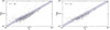 |
Fig. C.1. Dependence of a Compton-Y parameter between ComPACT and PSZ2 catalogue. The purple line represents the scaling relation defined by Equation C.1. The light purple band shows the 1σ scatter. Grey points mark individual measurements from the PSZ2 catalogue. Left panel: Measurements in the yPlanck map. Right panel: Measurements in the yACT+Planck map. |
Appendix D: Catalogue simulation
In this section, we provide a completeness estimation to illustrate the performance of our catalogue across different mass and redshift ranges. The completeness has been evaluated by injecting simulated clusters into the real ACT+Planck maps and applying the deep learning algorithm to them. We generate parameters for galaxy clusters on a redshift grid that uniformly covers the range 0.2 < z < 2. The minimum halo mass is set to M500c > 8 × 10¹³ M⊙. In total, we made one million samples of simulates clusters.
For a given redshift and mass, we compute the gas pressure profile describing the electron pressure distribution in the intracluster medium, using the universal gNFW profile (Nagai et al. 2007):
![Mathematical equation: $$ P(\xi ) = P_{500} \times \frac{P_0}{(c_{500} \xi )^{\gamma } [(1 + (c_{500}\xi )^\alpha )]^{(\beta - \gamma )/\alpha }}, $$](/articles/aa/full_html/2026/07/aa59201-26/aa59201-26-eq5.gif)
where P0 = 8.401, c500 = 1.177, γ = 0.3081, α = 1.0510, and β = 5.4905, as derived in Arnaud et al. (2010). The normalisation factor, P500, is computed following the same scaling relations and methodology presented in Arnaud et al. (2010).
Next, the pressure profile is interpolated onto a 64 × 64 pixel grid in a plate carrée projection and placed at a random position on the ACT+Planck intensity maps. The 64 × 64 pixel grid is chosen to ensure that the deep learning model can analyse the cluster surroundings and apply area-based detection criteria. This process is performed separately for three frequencies: 97.8 GHz, 149.8 GHz, and 220 GHz.
For each cluster, we calculate per-pixel predictions on a 32 × 32 grid centred on the cluster position (because the model input in Voskresenskaia et al. 2024 has a size of 32 × 32 pixels). We apply the minimal threshold of pthr > 0.3 to suppress noise (see Voskresenskaia et al. 2024) and identify the nearest connected group of pixels, characterised by its maximum probability (pmax) and area (S). The detection thresholds are pmax > 0.8 and S > 20 (see Figure 5 in Voskresenskaia et al. 2024).
All Tables
Number and percentage of candidates that are classified in the three different classes in full catalogue and in priority I.
Sample of massive galaxy clusters detected by the zCluster or Zaznobin algorithms.
All Figures
|
Fig. 1. Comparison of cluster redshift estimates obtained with the Zaznobin method and with zCluster. Left: Cumulative redshift distribution of cluster candidates obtained with the Zaznobin method and with zCluster. The Zaznobin method is especially effective for low-redshift systems (z < 0.2), whereas zCluster is able to recover clusters out to higher redshifts (z ≳ 0.8). Right: Distribution of the photometric redshift error, δz/(1 + zspec), for clusters with spectroscopic redshifts. |
| In the text | |
|
Fig. 2. Estimated completeness of the DL based cluster catalogue (without Planck SZcat selection) in the (M500c, z) plane. The black dashed line corresponds to detection thresholds of pmax > 0.8 and S > 20. The white dash-dotted line represents the average mass evolution of a 2 × 10¹⁵ M⊙ cluster over redshift (from Fakhouri et al. 2010). Left panel: Within the ACT DR5 footprint (13 211 deg2). The black dashed contour shows the 90% completeness of the catalogue, while the solid yellow line marks the same level for the ACT DR5 S/N > 3 catalogue at matched purity. The ComPACT achieves higher completeness than ACT DR5S/N > 3 at fixed purity, especially for massive clusters at high redshift, while both catalogues perform comparably at low z. Right panel: Outside the ACT DR5 footprint (∼3000 deg2). Catalogue retains high completeness for massive clusters across the redshift range, demonstrating its potential to identify new systems beyond existing survey coverage. |
| In the text | |
|
Fig. 3. Comparison of the ComPACT cluster sample in the mass–redshift plane. The distribution of ComPACT clusters is shown alongside those from ACT DR6 (purple contours), PSZ2 (blue contours), and SPT-DEEP (orange contours). The dashed lines trace the mass evolution of 2 and 3 × 10¹⁵ M⊙ clusters at z = 0 for a fixed cosmology (Fakhouri et al. 2010). Circles indicate clusters with redshifts from the literature (Table 1), while stars denote clusters with newly determined redshifts. Colours distinguish cluster categories: grey points mark ComPACT clusters with literature mass measurements, green points indicate new mass estimates from Planck y-maps, and magenta points show new mass estimates from ACT+Planck y-maps. Clusters with newly determined redshifts and masses are highlighted in green. Orange points above the 2 × 10¹⁵ M⊙ line represent clusters from the catalogues listed in Table 1 that are not included in ComPACT. |
| In the text | |
|
Fig. 4. Most massive clusters that are detected by zCluster or Zaznobin algorithms on z = 0.2, 0.69 and 1.2. Each panel shows an optical RGB image from the DESI Legacy Imaging Surveys with overlaid SZ–detection contours. For y-maps, contour levels correspond to μ + σ × {3, 4…}, where μ and σ are estimated locally within an annulus around each cluster, as described in Sect. 4. Contour labels indicate the corresponding significance level in units of σ. |
| In the text | |
|
Fig. B.1. Fraction of random fields for which the corresponding detection statistic exceeds a given threshold. In each panel, the grey line shows the fraction for random positions. The red dashed line indicates the ACT DR5 candidate sample, while the blue dashed line corresponds to PSZ2. Left panel: Distribution of the zCluster density contrast statistic δ for random positions. We find that 5% of the random fields have δ > 3. Middle panel: Distribution of S/N values in yPlanck maps. We find that 5% of random positions have S/N > 1.7. Right panel: Distribution of S/N values in yACT+Planck maps. Selection threshold is S/N > 2. All catalogues are restricted to the ACT DR5 footprint. |
| In the text | |
|
Fig. C.1. Dependence of a Compton-Y parameter between ComPACT and PSZ2 catalogue. The purple line represents the scaling relation defined by Equation C.1. The light purple band shows the 1σ scatter. Grey points mark individual measurements from the PSZ2 catalogue. Left panel: Measurements in the yPlanck map. Right panel: Measurements in the yACT+Planck map. |
| In the text | |
Current usage metrics show cumulative count of Article Views (full-text article views including HTML views, PDF and ePub downloads, according to the available data) and Abstracts Views on Vision4Press platform.
Data correspond to usage on the plateform after 2015. The current usage metrics is available 48-96 hours after online publication and is updated daily on week days.
Initial download of the metrics may take a while.