


| Issue |
A&A
Volume 710, June 2026
|
|
|---|---|---|
| Article Number | A382 | |
| Number of page(s) | 17 | |
| Section | Planets, planetary systems, and small bodies | |
| DOI | https://doi.org/10.1051/0004-6361/202659897 | |
| Published online | 01 July 2026 | |
A microphysical thermal model for the lunar regolith: Determining the lunar regolith properties using a combination of LRO/Diviner and Chang’E-2/MRM data
1
Institute of Geophysics and Extraterrestrial Physics (IGEP), Technische Universität Braunschweig,
Mendelssohnstr. 3,
38106
Braunschweig,
Germany
2
Planetary Science Institute,
1700 East Fort Lowell,
Tucson,
AZ
85719,
USA
3
Hawai‘i Institute for Geophysics and Planetology, University of Hawai’i at Mãnoa,
1680 East-West Road, POST Building 602,
Honolulu,
HI
96822,
USA
★ Corresponding author: This email address is being protected from spambots. You need JavaScript enabled to view it.
Received:
16
March
2026
Accepted:
10
May
2026
Abstract
Context. The surface of the Moon is covered by regolith and its microphysical structure is not only linked to surface processes and regolith evolution, but is also important for in situ resource utilization and mission planning.
Aims. We aim to uniquely constrain lunar regolith grain size and density stratification for the highlands and to further investigate the latitudinal dependence of regolith properties using remote sensing data.
Methods. We matched simulated surface and microwave brightness temperatures with Lunar Reconnaissance Orbiter/Diviner and Chang’E-2/Microwave Radiometer measurements. The physical temperatures of the regolith were modeled by applying a microphysical thermal model that more directly simulates physical properties of the regolith, such as grain size and volume filling factor.
Results. First, we find that the regolith-density stratification and grain size can only be unambiguously constrained by using both Diviner and Microwave Radiometer measurements due to their complementary wavelength ranges. The global regolith grain radius for equatorial highlands was determined to be 45−4+6 µm and the bulk density in the deeper regolith layers was found to be 1800-90+70 kg m−3. Second, the combined analysis of the latitudinal dependence up to ±80° latitude suggests a decrease in bulk density with increasing latitude. We also show that the previously proposed variation in the solar-incidence-angle-dependent albedo is not compatible with microwave brightness temperatures at higher latitudes.
Key words: methods: numerical / Moon / planets and satellites: surfaces
© The Authors 2026
 Open Access article, published by EDP Sciences, under the terms of the Creative Commons Attribution License (https://creativecommons.org/licenses/by/4.0), which permits unrestricted use, distribution, and reproduction in any medium, provided the original work is properly cited.
This article is published in open access under the Subscribe to Open model. This email address is being protected from spambots. You need JavaScript enabled to view it. to support open access publication.
1 Introduction
Regolith is the layer of fragmented debris covering the lunar surface (e.g., Langevin & Arnold 1977; McKay et al. 1991), formed by the gradual breakdown of bedrock over time due to meteoroid bombardment, space weathering (Pieters & Noble 2016), and thermal processes (Delbo et al. 2014). During the Apollo era, the regolith was characterized by several in situ experiments and laboratory measurements of returned samples. More recently, the Chang’E 3–6 and Chandrayaan-3 missions helped to further characterize the lunar regolith by investigating previously unsampled regions, such as higher latitudes and the lunar farside via robotic landers, rovers, and sample return. In addition to in situ measurements and sample return, remote sensing measurements offer a powerful tool for characterizing lunar regolith. They enable the characterization of regolith properties on a global scale, but models are often required to interpret the measurements. Radiometric measurements of the thermal emission of the lunar surface and subsurface can be interpreted using thermal models and allow the microphysical structure of the regolith, such as bulk density and grain size, to be determined.
The thermal emission of the lunar surface has been measured in the infrared by the Diviner Lunar Radiometer Experiment (Diviner) on board the Lunar Reconnaissance Orbiter (LRO) and in the microwave range by the Microwave Radiometer (MRM) on board the Chang’E-2 (CE-2) orbiter. While the Diviner measurements are sensitive to the thermal emission from the surface, MRM measurements are more sensitive to thermal emission from deeper regolith layers due to their longer wavelengths and can therefore constrain the subsurface temperature profile. To interpret the radiometer data, most studies apply thermal models based on the heat1d-model by Hayne et al. (2017), who use the empirical H-parameter to describe the variation in bulk density and thermal conductivity with depth (Vasavada et al. 2012). However, there are only a few studies that have simultaneously fit both Diviner and MRM data. Feng et al. (2020) and Siegler et al. (2020) applied the heat1d-model to fit both the Diviner channel 7 and MRM data and derived updated thermal and electromagnetic properties of the regolith. Building upon this model, Wei et al. (2020) added a mixture of regolith with rocks and derived the volumetric rock abundance at several rocky areas. Chen et al. (2024); Zheng et al. (2025) characterized the regolith of selected craters at the pole using both datasets.
Bürger et al. (2024) developed a one-dimensional microphysical thermal model (“1DMTM”) that more directly simulates regolith properties, such as grain size and volume filling factor. However, the free parameters in the microphysical thermal model cannot be uniquely constrained when they are only compared with Diviner infrared measurements (Bürger et al. 2024).
Therefore, the goal of this work is to use not only the Diviner infrared measurements but also the MRM microwave measurements to determine the stratigraphy and grain size of the lunar regolith with the microphysical thermal model. We also revisit the latitudinal dependence of lunar regolith properties discussed previously in Bürger et al. (2024).
This paper is organized as follows. Section 2 introduces the MRM and Diviner data and Sect. 3 gives an overview of the applied microphysical thermal model and radiative transfer model used to derive synthetic brightness temperatures. Section 4 presents and discusses the derived regolith properties for the equatorial highlands and the latitudinal gradient. Finally, Sect. 5 summarizes the study.
2 Dataset
2.1 CE-2 Microwave Radiometer brightness temperatures
2.1.1 Instrument and calibration
MRM (also referred to as the Chang’E Lunar Microwave Sounder, CELMS) on board the CE-2 orbiter is a four-channel microwave radiometer with channel frequencies of 3.0, 7.8, 19.35, and 37 GHz (corresponding wavelengths of 10, 3.8, 1.6, and 0.8 cm) (Feng et al. 2013; Wang et al. 2010; Zheng et al. 2019). The absolute accuracy of the radiometer is 0.5 K (Wang et al. 2010). CE-2 is a copy of the CE-1 orbiter and the CE-2 mission was in operation from October 2010 to May 2011. The mission was in a polar orbit with an altitude of 100 km and the instrument had a nadir view resulting in a resolution on the lunar surface of approximately 25 km for the 3 GHz channel and 17.5 km at the other frequencies. The instrument was calibrated using a two-point calibration by repeatedly observing a cold target (cold space with 2.7 K) with an additional set of calibration horns and an internal hot target (Wang et al. 2010). In recent years, evidence of thermal contamination of the cold target, in conjunction with a calibration issue of the microwave measurements, arose (Feng et al. 2020; Hu et al. 2017). First, the main-lobe of the cold reference antenna observing cold space also received radiation from the lunar surface during calibration, which resulted in lower antenna temperatures after calibration (Hu et al. 2017). This effect is strongest in the two lowest frequency channels 3.0 and 7.8 GHz due to their larger main-beam widths. However, later Hu & Keihm (2021) showed that the contamination by the lunar surface thermal emission is inadequate to explain the observed large offsets in the low-frequency channels and suggest focusing on uncertainties in the preflight derivation of hardware loss coefficients. Second, there is an additional discrepancy at 6 a.m. and 6 p.m. local time, when the spacecraft was in the terminator orbit and the calibration horn pointed toward the Sun (Feng et al. 2020). Again, this effect is strongest for the low-frequency channels because of their larger horns. Although empirical corrections have been suggested to correct the low-frequency data (e.g., Hu et al. 2017; Siegler et al. 2020), we base our study only on the measurements in the 19.35 and 37 GHz channels, which are believed to have a more robust absolute temperature calibration (Feng et al. 2020; Siegler et al. 2020). The MRM measurements are sensitive to the subsurface thermal emission with the penetration depth being controlled by the measurement frequency and the dielectric properties of the lunar regolith (see Sect. 3.2). Siegler et al. (2020) estimated the depth over which 99% of the total radiation is emitted for the lunar highlands to be ∼0.3 m for the 37 GHz channel and ∼0.7 m for the 19.35 GHz channel.
2.1.2 Antenna and brightness temperatures
This study uses the MRM Level 2C dataset, which has undergone system calibration and geometric correction. Wang et al. (2010); Zheng et al. (2012) provide more details on the processing and calibration of the dataset. The thermal emission measurements of MRM are reported as calibrated antenna temperatures, describing the received power from the target.
Under the idealized assumption of a uniform source that fully fills the telescope beam and in the absence of instrument-dependent effects (e.g., spillover, efficiency losses), the antenna temperature, TA, is related to the Planck brightness temperature, TB, by the following equation (e.g., Choukroun et al. 2015; Frerking et al. 2019; Redman et al. 1992)
 (1)
(1)
where f is the channel frequency, k the Boltzmann constant, and h the Planck constant. This means that the antenna temperature does not always correspond to the Planck brightness temperature of the source. Only when the Rayleigh-Jeans limit applies, the antenna temperature converges to the Planck brightness temperature. Because the frequencies of MRM’s channels are relatively low, the difference between the antenna and Planck brightness temperature ∆T = TA − TB is rather small with ∆T ≈ −0.5 K and ∆T ≈ −0.9 K for the 19.35 GHz and 37 GHz channel, respectively. However, as this is not completely negligible with respect to the measurement uncertainty of MRM and the standard deviation of the later averaged and binned MRM measurements, we included this correction. We applied Eq. (1) and solved for the Planck brightness temperature, TB, at each frequency of interest. Again it is important to note that this spectral correction is based on the assumption of a uniform blackbody target. Previous works (e.g., Feng et al. 2020; Wang et al. 2010; Zheng et al. 2012) refer to the MRM Level 2C data as brightness temperatures without applying this spectral correction.
Second, it is important to note that the MRM Level 2C data should be interpreted as antenna-pattern-weighted values instead of fully pattern-deconvolved brightness temperatures. The difference becomes negligible only in the case of a uniform brightness temperature across the footprint of the instrument. In reality, however, the brightness temperature of the lunar surface is not uniform and varies spatially. Therefore, if there are multiple brightness temperatures in the antenna’s field of view, these are weighted according to the beam pattern, which is illustrated in Wang et al. (2010) and Siegler et al. (2023, their Extended Data Fig. 2), and deconvolution would be required to obtain local brightness temperatures. This process is computationally intensive. Most recently, St. Clair et al. (2024) published MRM brightness temperature maps derived by deconvolving the antenna-pattern-weighted measurements. However, since the maps were derived using 2-hour local time bins, we did not use them in this study because we are interested in time series data with higher temporal resolution. This is why we continue with the antenna-pattern-weighted, but Planck-equivalent brightness temperatures obtained from the inverse of Eq. (1). We must bear in mind that there may be differences between the antenna-pattern-weighted and fully pattern-deconvolved brightness temperatures due to the antenna beam pattern.
2.1.3 Data filtering
The MRM measurements were filtered for the best quality by applying a filter based on (a) albedo, (b) rock abundance, and (c) local slope. First, the data were filtered by albedo to reduce uncertainties in the microwave measurements due to albedo variations. We selected only those pixels that are within (0.99, 1.01) × (1 − An) with An being the normal albedo measured by the Lunar Orbiter Laser Altimeter (LOLA; Lucey et al. 2014; Smith et al. 2010). In addition, the albedo filter allows one to distinguish between maria and highlands as both exhibit a characteristic difference in normal albedo with mean values of An,M = 0.17 and An,H = 0.31. Second, the data were filtered by rock abundance. Rocks on the lunar surface have a higher thermal inertia than the lunar regolith and therefore heat-up and cool-down slower during the day and stay warmer during the night. The rocks contribute to the measured thermal emission and thus, to learn about the regolith, we should select only those regions with a low rock abundance. Bandfield et al. (2011, 2017) derived the rock abundance on the lunar surface up to ±80° latitude using the thermal emission measurements in multiple infrared channels from Diviner (Paige et al. 2010) and found a global average rock abundance of 0.4%. We therefore only selected those pixels with a rock abundance <0.4%. Third, a filter based on the north-south slope of each pixel was applied with slope <1° to reduce the influence of topography. After filtering the data as described above, we applied another correction to the data to analyze it as a function of latitude. Due to the relatively short measurement period, seasonal influences are visible in the data. Therefore, we calculated an effective latitude for each measurement by taking the subsolar latitude into account.
Finally, the data were filtered by latitude and binned as a function of local time with a bin size of 0.5 hours. We created two different datasets to analyze in this study: (a) highlands at the lunar equator, i.e., all filtered data within ±1° latitude, and (b) highlands as a function of latitude up to ±80° with a bin size of ±0.5°. For the equatorial dataset, a two-times larger latitude band was selected to capture a greater number of measurements, because these are sparser at the equator compared to higher latitudes.
2.2 LRO Diviner regolith temperatures
Diviner on board LRO is a nine-channel solar and infrared filter radiometer (Paige et al. 2010). The instrument has measured the thermal emission of the lunar surface in high resolution since 2009 and global day- and nighttime brightness temperature maps have been created (Powell et al. 2023; Williams et al. 2017). In this study, we used the same dataset as in our previous study (Bürger et al. 2024), to – when combined with the CE-2/MRM brightness temperatures – further constrain the previously investigated regolith properties. The dataset is based on the regolith temperatures derived by Bandfield et al. (2011, 2017), where the effect of surface rocks is separated from regolith. The filtering of the regolith temperatures for the best data quality (similar to Sect. 2.1.3) is described in Bürger et al. (2024) and their Fig. 1 shows the resulting mean Diviner regolith temperatures as a function of latitude. It is important to note that the regolith temperatures are only available between local times of 7:30 p.m. and 5:30 a.m. However, this is not a problem because nighttime temperatures are most sensitive to regolith thermal conductivity and bulk density, while these properties have a negligible effect on daytime temperatures.
3 Models
This section describes the two models required to produce synthetic brightness temperatures. First, the temperature of the regolith is modeled as a function of depth by applying a thermal model. The physical temperatures are then converted into a brightness temperature by applying a radiative transfer model.
3.1 Microphysical thermal model
This study uses the microphysical thermal model presented in Bürger et al. (2024). This thermal model expands upon previous models by more directly simulating regolith properties, such as volume filling factor and regolith grain size. The evolution of the temperature, T, as a function of depth, x, and time, t, is described by the one-dimensional heat transfer equation
 (2)
(2)
which takes as input the physical and thermophysical properties of the regolith. All properties and thermal model parameters are explained in great detail in Bürger et al. (2024). The thermal conductivity, λ, is modeled as a function of temperature, grain radius, and volume filling factor (Gundlach & Blum 2012). The specific heat capacity, cp, is a temperature-dependent property. The depth-dependency of the bulk density, ρ(x), is described by the model of Schräpler et al. (2015). This model is based on the assumption that the pressure in the regolith is determined by the lithostatic stress and therefore the regolith is compacted by the weight of the overlying regolith layers. The model describes the bulk density as a function of regolith grain radius, r, grain density, ρgrain, surface density, ρs, deep layer density, ρd, and logarithmic transition width, ∆. The depth at which the transition from low to high bulk density occurs decreases with increasing grain radius. The transition width determines the steepness of the transition from the loose packing at the surface to the maximum bulk density in the deeper layers. The steepness decreases with increasing transition width. The bulk density, ρbulk, and volume filling factor, ϕ, are related via the grain density, ρgrain, of the material:
 (3)
(3)
We would like to point out that the equations in Schräpler et al. (2015) contain several errors, which have been corrected in the revised version by Bürger et al. (2024). Bürger et al. (2024) also discuss two different calibrations of the turnover pressure (low and high turnover pressure, their Fig. 2), which has been identified as a critical but rather uncertain parameter. The turnover pressure, pm, is the formal inflection point of the ϕ(log p) curve and is interpreted as the critical restructuring pressure of the regolith packing. Its absolute calibration and dependence on the grain radius are crucial for deriving lunar regolith grain radii with the help of the thermal model (for a more detailed discussion, see Sect. 4.1.4 in Bürger et al. 2024). Most recently, Blum et al. (2026) investigated the relationship between turnover pressure and grain size and found that it follows a power law with slope –2 as suggested by the theoretical model of Tatsuuma et al. (2023). We used the result of Blum et al. (2026),
 (4)
(4)
to constrain the turnover pressure in the thermal model. Here, r represents the grain radius and A the Hamaker constant. Silica has a mass fraction of ∼45% in highland lunar regolith (McKay et al. 1991) and we assume A = ASiO2 in this study. This function is quite similar to the lower turnover pressure calibration in Bürger et al. (2024) in the relevant grain radius range of 10–100 µm. However, we still expect changes in the simulated temperatures because the thermal model is very sensitive to this parameter. Outside the above mentioned radius range there will be larger differences because Schräpler et al. (2015) proposed the grain-size dependency of the turnover pressure follows a power law with slope −4/3.
The lunar highlands are defined in the thermal model by a bolometric Bond albedo at zero solar incidence angle of A0 = 0.12 (Feng et al. 2020), a grain density of 2880 kg m−3 (mean of Kiefer et al. 2012), and a geothermal heat flux of Q = 0.008 W m−2 (Siegler et al. 2022). The bolometric Bond albedo is a function of solar incidence angle, and unless otherwise specified, the parameterization from Feng et al. (2020) is used in the thermal model. To account for the geothermal heat flux, Q, the lower boundary condition of the thermal model was updated and reads
 (5)
(5)
with TN and xN being the temperature and depth of the bottom layer, respectively.
In our previous study, we only analyzed surface temperatures and therefore required a relatively short equilibration time of the model of ∼2 years (Bürger et al. 2024). For the modeling of the microwave brightness temperatures, subsurface temperatures are also relevant and therefore a longer equilibration time is required. The thermal model was run for ∼20 years to equilibrate the subsurface temperatures and to remove the effect of the temperature initialization. By choosing an appropriate initial temperature profile (see e.g., Bürger et al. 2024; Hayne et al. 2017) equilibration times can be kept relatively short. Convergence was ensured for all latitudes and comparison of the temperature profiles with a run for ∼75 years yielded a RMSD < 0.1 K. The model used a non-uniform grid with equal grid spacing in logarithmic space. Within the grid setup, the grid spacing near the surface has the greatest influence on the simulated microwave brightness temperatures. We chose a finer grid spacing between the first two grid points of ∆x0 = 1 mm, while the total depth of the simulation was set to xN = 1 m and the number of grid points to N = 100.
3.2 Radiative transfer model
The applied radiative transfer model is described in detail in Feng et al. (2020); Siegler et al. (2020) and is based on the work by Ulaby et al. (1981, 2014). The modeled microwave brightness temperature TB is obtained by convolving the microwave electrical loss with the modeled physical temperature profile T(x) of the lunar regolith over depth x. In the model, the microwave electrical loss is represented by a weighting function w(x), which characterizes the fractional contribution of each regolith layer to the total microwave brightness temperature,
 (6)
(6)
The discrete form of the equation reads
 (7)
(7)
with index i denoting the respective regolith layer.
The weighting function of each layer is defined as
 (8)
(8)
with Γ, κi, di, and Ri,i+1 being the surface reflectivity, the power absorption coefficient, the thickness of each layer and the reflection coefficient between two layers, respectively. The reflection coefficient between layer i and layer i + 1 reads
 (9)
(9)
with ϵ′ being the real part of the relative dielectric permittivity
 (10)
(10)
which is a function of bulk density, ρ, in grams per cubic centimeter (Carrier et al. 1991). Layer 0 is assumed to be vacuum and thus, the surface reflectivity reads
 (11)
(11)
The power absorption coefficient is a function of measurement frequency, f , the speed of light, c, the real part of the relative dielectric permittivity, ϵ′, and the loss tangent, tan δ
 (12)
(12)
The loss tangent is defined as the ratio of the imaginary and real part of the relative dielectric permittivity
 (13)
(13)
and is a function of bulk density, ρ, in grams per cubic centimeter, frequency, f, in gigahertz, and composition with b = 0.312, d = 0.0043, and c = −2.64 for highlands at 19.35 GHz and 37 GHz as derived in Feng et al. (2020). In general, the loss tangent is found to be significantly influenced by the FeO and TiO2 content of the material (Carrier et al. 1991). However, given the low levels of these elements in the highlands, their influence can be neglected here.
Thus, the penetration depth and therewith the amplitude of the diurnal variation in microwave brightness temperature depend on both the measurement frequency and the dielectric properties of the regolith. To first order, the behavior can be understood by considering the absorption coefficient in Eq. (12). First, the absorption coefficient scales roughly linearly with frequency. Because the loss tangent exhibits a small but non-negligible frequency dependence in the investigated frequency range, κ( f ) increases slightly faster than linearly with f. Consequently, the penetration depth (∝ 1/κ) decreases with increasing frequency and is therefore larger at lower frequencies. Because the lunar diurnal temperature variation is strongest at the surface and decreases with depth, the 19.35 GHz channel is expected to exhibit a lower diurnal brightness-temperature amplitude than the 37 GHz channel. Second, the loss tangent itself strongly affects the penetration depth: a larger imaginary part of the dielectric permittivity, and thus a higher loss tangent, increases absorption (dielectric loss) and therewith leads to a decrease in penetration depth and a larger diurnal brightness-temperature amplitude.
4 Results and discussion
4.1 Equatorial highland regolith
4.1.1 Constraining regolith properties using LRO/Diviner and CE-2/MRM data
In our previous study (Bürger et al. 2024), we derived lunar regolith properties by comparing simulated surface temperatures with nighttime regolith temperatures measured by the Diviner radiometer. However, there was a degeneracy among the three free parameters, the grain radius, r, the transition width, ∆, and the deep layer density, ρd, and therefore the solutions were non-unique. Due to the updated turnover pressure function (see Sect. 3.1, Eq. (4)), the thermal model calculations for the whole parameter space investigated in Bürger et al. (2024), namely r = 10, 20,…, 100 µm, ∆ = 0.1, 0.2,… 1.2, and ρd = 1500, 1600,… 2500 kg m−3, were repeated. Therefore, in a next step, the simulations were not only compared with the MRM data, but also again with the Diviner data. First, the resulting root-mean-square deviation (RMSD) was calculated:
 (14)
(14)
with the measured (brightness) temperature, Tn, simulated (brightness) temperature,  , and number of compared (brightness) temperature pairs, N. This was done separately for the Diviner data, the MRM 37 GHz data as well as the MRM 19.35 GHz data and their respective simulations. In a next step, as a measure for the theoretical best fit, a polynomial was fit to the measured data and the resulting RMSDpol was calculated to account for the intrinsic noise of the data. Details about the polynomial fit are given in Appendix A. Finally, the factor, Ω, by which the simulations deviate from the theoretically best possible solution (characterized by the respective polynomial; see Appendix A) was calculated using
 (15)
(15)
with i = 1, j = 1, and k = 1 for solutions based on the comparison with Diviner, i = 2, j = 2, and k = 3 for solutions based on the comparison with MRM 37 GHz and 19.35 GHz, and i = 3, j = 1, and k = 3 for solutions based on the comparison with all three datasets. Ω = 1 would mean that the simulation is as good as the theoretical best fit determined by fitting the polynomials to the data.
The result is displayed in Fig. 1 in the form of heat maps. For Diviner we observe the same pattern as in Bürger et al. (2024): the solutions are degenerate and increasing the deep layer density and the transition width, while slightly decreasing the grain radius, leads to multiple good fits to the data. The heat map for the MRM data also shows non-unique solutions within the investigated parameter space. Here, the interpretation is more complex, as the brightness temperatures are calculated from the temperature-depth profile and the radiative transfer model, both of which are influenced by the three free parameters. As a result, we note that neither the Diviner nor the MRM data alone can be used to unambiguously constrain the regolith properties. The combination of both datasets is needed for a unique solution and is illustrated in the two lower rows of Fig. 1. First, we note that for Diviner the similarly well-fitting parameter sets with higher deep layer densities (ρd ≥ 2000 kg m−3) result in simulated brightness temperatures that are systematically too cold in both the MRM 19.35 GHz and 37 GHz channel. Second, the lower deep layer densities (ρd ≤ 1600 kg m−3) resulting in multiple good solutions for the MRM channels, lead to simulated Diviner surface temperatures that are systematically too cold. Furthermore, the combined heat maps reveal that the solution space for the grain radius can be restricted to r = 40–60 µm and ∆ = 0.1–0.5 for the transition width. To identify the parameter set, which simultaneously fits the Diviner and both MRM measurements best, we had to increase the resolution for this restricted parameter space, and chose a four times higher resolution for the transition width, ∆, and the deep layer density, ρd, and a ten times higher resolution for the grain radius, r. The result is illustrated in the lowermost row of Fig. 1 and the best-fitting and unique solution can be identified as r = 45 µm, ∆ = 0.35, and ρd = 1800 kg m−3. Fig. 2 illustrates for this parameter set the simulated surface and microwave brightness temperatures, along with the corresponding Diviner and MRM measurements, showing very good agreement in all cases. We also estimated the error of the derived parameter set and derived  µm,
µm,  , and
, and  kg m−3. The error estimation is detailed in Appendix B. In the following subsection, the derived regolith properties are discussed and compared with literature values.
4.1.2 Comparison to literature values
Grain radius. Analysis of the returned Apollo samples revealed that the regolith particles follow a log-normal distribution, spanning from a few micrometers to several millimeters (McKay et al. 1991). Median particle radii (in mass) range from ∼20 to 136 µm (including >1 mm particles; Carrier 1973; Heiken et al. 1973; McKay et al. 1974), with most median values falling between ∼20 and 50 µm (McKay et al. 1991). The regolith grain radius of 45 µm derived in this study lies within this range. Of all the Apollo missions, the Apollo 16 mission is most representative for highlands, and the samples there have median grain radii between 27 and 136 µm (Heiken et al. 1973). The median grain radius (in mass) for the CE-5 and CE-6 regolith samples was determined to be ∼26 µm (Li et al. 2022) and ∼17.5 µm (Li et al. 2024), respectively. Finally, the derived grain radius of 45 µm is compared with another modeling result. Yu et al. (2025) applied a thermal model similar to Bürger et al. (2024), but with a difference in the absolute values of thermal conductivity and the turnover pressure, and chose only the grain radius as a free parameter. They derived a global grain radius map by comparing modeled temperatures with Diviner bolometric temperatures and found a mean grain radius of 55 µm.
Stratification. The derived deep layer bulk density of ρd = 1800 kg m−3 translates into a deep layer volume filling factor of ϕd = 0.625. As already discussed in Bürger et al. (2024), a lower limit of the deep layer volume filling factor is given by ϕ = 0.56 for random loose packing (RLP) (Onoda & Liniger 1990), while random close packing (RCP) of monodisperse spheres gives an upper limit of ϕ = 0.64 and the maximum volume filling factor increases with increasing polydispersity. The derived deep layer volume filling factor for the equatorial highland regolith lies well within this interval given by RLP and RCP for monodisperse particles.
The returned Apollo 15–17 drill cores showed regolith bulk densities in the range 1470–1990 kg m−3 (Carrier 1974), while the Apollo 15–17 core tubes ranged from 1360 kg m−3 to 2290 kg m−3 (Carrier et al. 1991). Moreover, based on the Apollo 15–17 core tube samples, Mitchell et al. (1974) derived best estimate values for the regolith bulk density of 1580 ± 50 kg m−3 for the depth interval 0–30 cm and 1740 ± 50 kg m−3 for the depth interval 30–60 cm. Figure 3 illustrates the derived bulk density profile together with the constraints listed above. We note an acceptable agreement, although with the caveat that most of the core tubes and drill cores originate from the lunar maria and not the highlands.
Another constraint on the derived stratification profile is the depth of astronaut footprints on the lunar surface. An analysis of more than 700 actual footprints from astronauts on the lunar surface showed that the average bootprint depth is approximately 0.8 cm (calculated from Fig. 3–18 in Mitchell et al. 1974). Following the recipe in Sect. 6 in Blum et al. (2026) we calculated the depth of astronaut footprints on the lunar surface using the regolith properties derived in this study and obtain a bootprint depth of 0.79 cm, which agrees with the actual footprint depths.
Finally, we note that the derived transition width ∆ = 0.35 lies slightly outside the interval ∆ = 0.4–0.6, which was found in Blum et al. (2026) for granular packings of moderately wide size distributions with r90ν/r10ν ≲ 10, with r90ν and r10ν being the 90th and 10th percentiles of the cumulative volume-based grain size distribution. Values of ∆ ≳ 1 are suggested for packings with r90ν/r10ν ≳ 10 (Blum et al. 2026). In conclusion, the stratification profile derived in this study from Diviner and MRM data is consistent with the principles of granular packing, bulk densities from Apollo drill cores as well as core tubes, and the depth of astronaut footprints.
 |
Fig. 1 Derived regolith properties for highlands at the lunar equator when comparing the simulations with Diviner regolith temperatures (top row) and MRM brightness temperatures (second row) and both combined (third and fourth row). The heat maps illustrate the factor, Ω, (for the definition see Eq. (15)) by which the simulations deviate from the theoretically best possible solution (the theoretical best fit would result in Ω = 1). There are three free parameters in the thermophysical model, the grain radius, r, the transition width, ∆, and the deep layer density, ρd. The heat maps show this factor, Ω, for the combinations of two of each of the three free parameters, with the third parameter being variable. For illustration purposes, all Ω > 5 are colored black. |
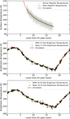 |
Fig. 2 Resulting simulated surface temperatures and microwave brightness temperatures (red lines), along with the Diviner (top), MRM 37 GHz (center) and MRM 19.35 GHz (bottom) measurements (individual: dots; binned: squares) as a function of local time. |
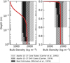 |
Fig. 3 Resulting bulk density profile (red line) along with constraints from returned drill cores and core tubes (boxes) (Carrier 1974; Carrier et al. 1991; Mitchell et al. 1974, see Sect. 4.1.2). Left: Logarithmic depth. Right: linear depth. |
4.1.3 Caveats
Although we filtered the data for low rock abundance, small rock fragments may still lie on the surface and be buried in the regolith. However, this work only models pure regolith, representing a simplification. The presence of buried rock fragments results in a larger amplitude of the microwave brightness temperatures, as the rocks reduce the effective penetration depth to which the microwave radiometer measurements are sensitive. This is due to their larger bulk density and the resulting increase in dielectric permittivity and loss tangent. For example, many rocky areas around young impact craters on the lunar surface are identified as cold spots at night and hot spots during the day in the microwave range due to this effect (Hu et al. 2018; Zhu et al. 2019). In addition, in their global loss tangent map for highlands, Siegler et al. (2020) found that areas with high loss tangents are associated with rocky impact craters. Although we exclude rocky areas, some small rock fragments may still be present, which can generally explain why the loss tangent derived by Feng et al. (2020); Siegler et al. (2020) for regolith in equatorial highlands with low rock abundance is still greater than the loss tangent determined experimentally from Apollo regolith samples (Carrier et al. 1991), as a less transparent regolith was needed to match the MRM measurements. In the radiative transfer model, the loss tangent influences the amplitude of the simulated brightness temperatures, but cannot systematically shift them to lower or higher temperatures. However, the latter would be necessary in our parameter study, for example for parameter sets with higher deep layer densities, in order to fit the MRM measurements.
We also would like to note that the measurements by Diviner are considered to be more reliable than those by MRM. This is due to the reported calibration issue in the 3 GHz and 7.8 GHz channels, as well as the uncertainties due to the antenna beam pattern and the larger footprint of MRM (see Sect. 2.1). However, quantifying these effects requires an in-depth understanding of the instrument and spacecraft operation and is beyond the scope of this study.
 |
Fig. 4 Comparison of the modeled regolith temperatures (black lines) and the Diviner regolith temperatures as a function of latitude for highlands. The lower panels show the resulting RMSD between the model and the measurement as a function of latitude ((c), (d) calculated in steps of 5° latitude; otherwise in steps of 1°). (a) Assuming constant regolith properties as derived for the lunar equator; (b) applying a variation in the solar-incidence-dependent albedo; (c) poleward decrease in the deep layer bulk density, and (d) poleward increase in the transition width. If not stated otherwise, the solar-incidence-dependent albedo after Feng et al. (2020) has been applied. |
4.2 Latitudinal dependence of lunar regolith properties
4.2.1 LRO/Diviner
Bürger et al. (2024) observed for the majority of the non-unique solutions a latitudinal gradient when comparing the simulated temperatures with Diviner regolith temperatures as a function of latitude up to ±80°. The modeled temperatures were systematically too warm at high latitudes and the onset of the gradient was observed around 40° latitude. Previous works based on Diviner data showed contrasting results – the H-parameter map by Hayne et al. (2017) did not show a latitudinal gradient, while a strong gradient was observed by Yu & Fa (2016) in their surficial thermal conductivity map. All of these works employed a different solar-incidence-angle-dependent albedo function. Bürger et al. (2024) showed that a variation in the solar-incidence-dependent albedo function is able to significantly reduce the observed latitudinal gradient. Their required albedo variation suggests a slightly lower albedo at low incidence angles and slightly higher albedo at high incidence angles than all other previous functions (Bürger et al. 2024, their Fig. 11). The incidence angle is defined here as the angle between the surface normal and the Sun. This supported the suggestion of Hayne et al. (2017) that the strong latitudinal gradient in Yu & Fa (2016) could be a solar-incidence-dependent albedo effect. Indeed, in a most recent work, Yu et al. (2025) derived a global grain radius map applying the albedo variation suggested in Bürger et al. (2024) and their maps did not exhibit a latitudinal gradient.
Bürger et al. (2024) only identified one set of regolith properties without the albedo variation that were able to describe the Diviner regolith temperatures reasonably well for all latitudes. However, this set of regolith parameters was based on the so-called “high turnover pressure calibration”, which does not match the turnover pressure as constrained by Blum et al. (2026) (see Sect. 3.1). Therefore, when applying the best fit of the equatorial highland regolith in this work (r = 45 µm, ∆ = 0.35, ρd = 1800 kg m−3, see Sect. 4.1.1; solar-incidence-angle-dependent albedo after Feng et al. (2020), see Sect. 3.1) to all latitudes up to ±80° we again identify the same latitudinal gradient for the Diviner regolith temperatures as seen before with the modeled temperatures being systematically too warm at higher latitudes. The gradient is illustrated in Fig. 4 and has an onset around 40° latitude and shows a RMSD ≳3 K at the highest latitudes. Figure 4 also illustrates the effect of the solar-incidence-dependent albedo variation suggested in Bürger et al. (2024). Finally, another option to reduce the latitudinal gradient investigated in Bürger et al. (2024) was the variation in intrinsic regolith properties with latitude, where a poleward decrease in bulk density was suggested. This can be achieved with a decrease in the deep layer bulk density or an increase in the transition width (see Fig. 4). These options will be discussed again in Sect. 4.2.3. Bürger et al. (2024) also showed that a variation in the grain radius cannot remove the latitudinal gradient. Thus, this option will not be investigated further.
4.2.2 CE-2/MRM
No study has yet explicitly investigated the latitudinal dependence of regolith properties based on MRM measurements. However, similar to this study, Feng et al. (2020) created filtered global MRM datasets for highlands at latitudes of 0°, 30°, and 70° and plotted their best fit based on equatorial Diviner and MRM data against the MRM data at these latitudes. Their Fig. 8 shows a systematic trend with the brightness temperatures being systematically too cold at 70° latitude in both the 19.35 GHz and 37 GHz channels. In this work we use the filtered MRM data for highlands as a function of latitude (see Sect. 2.1.3) to investigate the latitudinal gradient observed in the Diviner data further and to check whether we also find the systematic trend observed in Feng et al. (2020). We plotted the simulated brightness temperatures based on the regolith properties constrained from the equatorial highlands data (r = 45 µm, ∆ = 0.35, ρd = 1800 kg m−3, see Sect. 4.1.1; solar-incidence-angle-dependent albedo after Feng et al. (2020), see Sect. 3.1) against this dataset. The result is illustrated in Fig. 5 for the northern hemisphere. For better data quality, we divided the data between the northern and southern hemispheres, because the MRM measurements showed increased scattering at higher latitudes for the southern hemisphere. The result for the southern hemisphere is illustrated in Appendix C in Fig. C.1. We note that the simulated brightness temperatures are always within the scatter of the un-binned MRM data for all latitudes. Visual analysis of the simulated and measured brightness temperatures reveals too warm simulated daytime brightness temperatures at ≥±70° latitude in both channels and, in the 19.35 GHz channel, also during the night at ±80°. We note that our simulations do not show the systematic trend in Feng et al. (2020). To quantify the latitudinal dependence in this work, the RMSD resulting from the comparison of the simulated and measured microwave brightness temperatures is plotted as a function of latitude in Fig. 6. For the assumption of constant regolith properties, it shows an increase in RMSD starting around +50° latitude for the 37 GHz channel and around +60° latitude for the 19.35 GHz channel in the northern hemisphere. However, we also note that this gradient is much lower than the one observed for the Diviner regolith temperatures. While in the case of the Diviner regolith temperatures the RMSD increases by a factor of ∼20 from the equator (RMSD = 0.17 K) to the highest latitudes (RMSD ∼ 3.5 K), the RMSD for the 37 GHz and 19.35 GHz channel only increases by a factor of ∼3 and ∼6, respectively. We therefore conclude that the microwave brightness temperatures do not exhibit a dramatic latitudinal gradient.
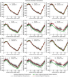 |
Fig. 5 Comparison of the modeled microwave brightness temperatures (solid lines) and brightness temperatures measured by MRM (dots: individual; squares: binned) as a function of latitude for the lunar highlands on the northern hemisphere. For illustration purposes only latitudes of 0°, +20°, +40°, +60°, +70°, and +80° (bin size ±0.5°) are plotted. Illustrated are the simulations assuming constant regolith properties (red lines) and the variation in the solar-incidence-dependent albedo (green stars). |
 |
Fig. 6 Resulting RMSD as a function of latitude when comparing the simulated microwave brightness temperatures with the MRM 37 GHz (top) and 19.35 GHz (bottom) data. Illustrated are the simulations assuming constant regolith properties (red line), applying a variation in the solar-incidence-dependent albedo (green stars), a poleward decrease in the deep layer density (blue crosses, calculated in steps of 5° latitude), or a poleward increase in the transition width (dashed orange, calculated in steps of 5° latitude), and the polynomial fit to the data (dash-dotted black). |
4.2.3 Discussion of latitudinal gradient
Variation in the solar-incidence-angle-dependent albedo. We explicitly investigated the effect of the solar-incidence-angle-dependent albedo variation suggested in Bürger et al. (2024) on the simulated microwave brightness temperatures and find that this leads to simulated subsurface temperatures, which are systematically too cold at higher latitudes. The effect is illustrated in Fig. 5 for the northern hemisphere and in Fig. C.1 for the southern hemisphere. The increased albedo at high incidence angles compared to previous albedo functions leads to microwave brightness temperatures that are too cold in both channels. The RMSD as a function of latitude in Fig. 6 shows for this case a strong increase in RMSD with increasing latitude. Another possibility to check whether the proposed solar-incidence-dependent albedo function is reasonable is the comparison of the simulated temperatures with Diviner daytime temperatures, because these are sensitive to albedo, but not to regolith thermophysical properties. Because the Diviner regolith temperatures used in this study are not available for daytime (Bandfield et al. 2011), we apply a different dataset: Feng et al. (2020) used Diviner channel 7 (25–41 µm) and 2 pixel per degree gridded measurements to represent the average surface temperature of the regolith and the measurements are filtered for low rock abundance and small slopes. The comparison of the simulated and mean channel 7 surface temperatures shows that the proposed albedo variation systematically underestimates the daytime temperatures at high latitudes. Therefore, we discard the albedo variation proposed in Bürger et al. (2024) in order to reduce the latitudinal gradient observed in the Diviner data.
Variation in the deep layer density. Another potential explanation for the observed latitudinal gradient in the Diviner regolith temperatures, as outlined in Bürger et al. (2024), is the variation in intrinsic regolith properties with a poleward decrease of the deep layer bulk density. Figure 7 shows the decrease in the deep layer density that is needed in order to minimize the latitudinal gradient for Diviner. The deep layer bulk density decreases from 1800 kg m−3 at the equator to 1590 kg m−3 at 80° latitude. Figures 6, 8, and C.2 illustrate the influence of this decrease on the modeled microwave brightness temperatures. We find that this results in a better agreement between the simulated and measured microwave brightness temperatures at higher latitudes during the daytime and thus overall lower RMSD values. However, there is a minor increase in simulated microwave brightness temperatures at night and this means that the already present discrepancy during night at ±80° latitude in the 19.35 GHz channel, with the simulated microwave brightness temperatures being too warm, cannot be removed. But the influence of topography is very strong at such high latitudes, so the data should not be treated as too significant. Figure 9 illustrates the factor Ω (Eq. (15)) as a function of latitude and shows that the variation in density of the deep layer yields Ω ≲ 2 for almost all latitudes. Thus, the poleward decrease in the regolith deep layer bulk density results in the best fit of the model for all latitudes and for both the Diviner and MRM data.
Variation in the transition width. The last option to be investigated is the poleward increase in transition width, ∆. Figure 7 shows the increase in the transition width that is needed in order to minimize the latitudinal gradient for Diviner. The value increases from 0.35 at the equator to 0.9 at 80° latitude. This leads to increased RMSD values for the microwave brightness temperatures at mid-latitudes up to ±70°, especially in the 19.35 GHz channel (see Fig. 6). Figs. 8 and C.2 reveal that the increase in transition width systematically underestimates the measured microwave brightness temperatures in the 19.35 GHz channel at these latitudes. We also note that the variation in the transition width leads to the best match with the measured microwave brightness temperatures at ±80° latitude. However, based on the overall fits, we conclude that this variation in transition width is less supported than the variation in deep layer density, but it cannot be as clearly ruled out as the variation in the solar-incidence-dependent albedo (see Fig. 9).
In situ measurements of the bulk density at high latitudes. Although the Apollo missions provide a large dataset on in situ bulk densities (see Sect. 4.1.2), all landing sites are located close to the equator at latitudes <30°. In 2023, as part of Chandra’s Surface Thermophysical Experiment (ChaSTE) on board the Vikram lander (69.373° S, 32.319° E) of the Chandrayaan-3 mission, a thermal probe was inserted into the regolith and the average bulk density at a depth of 10 cm was derived from the currents of the penetration motor as 1940 ± 10 kg m−3 (Mathew et al. 2025). This measurement is illustrated in Fig. 10 along with the bulk density profiles predicted in this study at 70° latitude. The decrease in deep layer density results in an overall decrease in bulk density for all depths, while the increase in transition width yields lower bulk densities for depths >1 cm, but shows increased bulk density values toward the surface. The bulk density estimated by ChaSTE does not support the prediction of a poleward decrease in bulk density and is even slightly higher than the derived equatorial bulk density. Mathew et al. (2025) note as a possible reason for the higher bulk density a modification of the regolith by the lander, for example, the uppermost dust layer may have been blown off during landing. The suggested poleward decrease in bulk density (see Fig. 10) will have to be tested further by future modeling efforts and upcoming lunar missions, whereby disturbances to the regolith must be kept to a minimum and measurement uncertainties must be small enough to resolve the predicted contrast of ∼200 kg m−3 at depths ≳10 cm. Relevant future payloads include, for example, the ProSEED drill (part of ESA’s payload package PROSPECT; Trautner et al. 2024), developed for a lunar polar lander mission and equipped with a permittivity sensor to measure regolith bulk density, and the lunar penetrating radar on board Chang’E-7 (Wang et al. 2024).
Mechanisms for the poleward decrease in the bulk density. We already discussed the latitudinal dependence of regolith formation and evolution processes in Sect. 4.2.1 of Bürger et al. (2024) and therefore only provide a brief summary here. First, one regolith formation process that can lead to compaction of granular materials is thermal cycling (Chen et al. 2006; Divoux 2010; Metzger et al. 2018). Figure 7 illustrates the decrease in diurnal temperature amplitude for different depths within the regolith as a function of latitude. The predicted poleward decrease in deep layer density or increase in transition width follow this pattern. Thus, the reduced diurnal temperature variations at higher latitudes could lead to a less compacted regolith. It is interesting to note that the volume filling factors corresponding to the deep layer bulk densities derived for the equatorial and high-latitude highland regolith, ϕd,0◦ ∼ 0.63 and ϕd,80◦ ∼ 0.55, are close to those for RCP (ϕ = 0.64) and RLP (ϕ = 0.56; Onoda & Liniger 1990) of monodisperse spheres (see Sect. 4.1.2). Because RLP represents the loosest possible random packing that is mechanically stable (Onoda & Liniger 1990), we speculate that thermal cycling could compact the regolith at the lunar equator from RLP toward RCP. However, one caveat is that it is unclear how the laboratory experiments on thermal cycling can be extrapolated to the lunar environment and millions to billions years of evolution. We note that thermal cycling cannot account for the increase in bulk density observed within the first centimeter of the subsurface for the less favored scenario of increased transition width (see Fig. 10).
Other regolith formation processes are space weathering and the reworking by larger impactors in the form of meteoroids. While the maximum flux of solar wind particles and micro-meteoroids occurs at the lunar equator (Cremonese et al. 2013), Robertson et al. (2021) predicted the opposite for larger impactors. Robertson et al. (2021) modeled asteroid collisions with the Moon and their corrected results (Robertson et al. 2023) showed that the flux of impacts to the lunar poles is 13% greater than the flux at the equator. This affects the regolith gardening rate, but considering the millions of years of exposure time, this should not significantly affect the physical properties. While Robertson et al. (2023) predicted that the mean impact angle also increases slightly from ∼44° at the equator to ∼49° at the poles, a significant change in impact velocity with latitude was not reported. In fact, the largest dependency of the impact velocity arises from the apex/antapex dichotomy due to the synchronous rotation of the Moon.
We conclude that, when discussing the effects listed above, thermal cycling provides a clear indication of a possible decrease in bulk density with increasing latitude. A detailed analysis of the effects of the listed latitudinal dependence of space weathering and meteoroid impacts on the regolith properties is beyond the scope of this study. We also note that while the poleward decrease in deep layer density provides the best model fit to the Diviner and MRM data in this work, it should be regarded as one possible interpretation of these data rather than an absolute statement about the properties of the lunar subsurface.
 |
Fig. 7 Predicted poleward decrease in deep layer density (top; blue line) and increase in transition width (bottom; orange line) based on the minimization of the latitudinal gradient for the Diviner regolith temperatures. Illustrated together with the poleward decrease in diurnal temperature amplitude in depths of 1 cm (dashed), 5 cm (dash-dotted), and 10 cm (dotted). The y axis of the diurnal temperature amplitudes is set to match the start and end values of the deep layer density or transition width variation. |
 |
Fig. 8 Same as Fig. 5, but for the simulations assuming a variation in deep layer density (blue crosses) and transition width (dashed orange). |
 |
Fig. 9 Factor Ω (defined by Eq. (15)) describing the deviation between our model and the theoretically best possible solution for the combination of Diviner and MRM as a function of latitude. Ω ≤ 2 is highlighted by the gray bar. |
 |
Fig. 10 Left: Comparison of the different predicted bulk density profiles at 70° latitude; constant regolith properties (solid line), variation in deep layer density (dashed line), and transition width (dash-dotted line). Illustrated together with the bulk density inferred from ChaSTE (cross) at ∼−69° latitude (Mathew et al. 2025). Right: Bulk density profiles resulting from the predicted poleward decrease in deep layer density in steps of 10° latitude and a start at 40° latitude. |
5 Conclusion
In this work, we uniquely constrained lunar regolith properties in the equatorial highlands by matching both LRO/Diviner regolith temperatures (see Sect. 2.2) and CE-2/MRM microwave brightness temperatures (see Sect. 2.1) with simulated surface and brightness temperatures. The measurements complement each other as the Diviner measurements are sensitive to the thermal emission from the surface, while the MRM measurements are more sensitive to the thermal emission from deeper layers. The regolith surface and subsurface temperatures were simulated using a microphysical thermal model (see Sect. 3.1), which simulates more directly regolith physical properties, such as grain radius and volume filling factor (Bürger et al. 2024). One important improvement in this work was the incorporation of the turnover pressure as constrained by Blum et al. (2026), which represents a critical but previously uncertain parameter in the thermal model. The radiative transfer model from Feng et al. (2020); Siegler et al. (2020) was used to derive the synthetic microwave brightness temperatures (see Sect. 3.2). In the second part of the paper, the latitudinal gradient identified in Bürger et al. (2024) for the Diviner regolith temperatures was discussed with the help of the additional MRM measurements. The key findings of this study are summarized in the following:
- 1a
The regolith-density stratification and grain size can only be unambiguously constrained when using both the LRO/Diviner (infrared) and CE-2/MRM (microwave) radiometer data (see Sect. 4.1.1), which have a complementary wavelength range;
- 1b
The regolith properties for lunar highlands at the equator are determined as follows: a grain radius of
 µm, a transition width in the density stratification profile of
  , and a deep layer density of
  kg m−3 (see Sect. 4.1.1). These values are in good agreement with literature values (see Sect. 4.1.2) and describe the highland regolith well for all latitudes <40°;
 - 2a
The modeled nighttime regolith temperatures exhibit a strong latitudinal discrepancy from the Diviner data with an onset around 40° latitude. The simulated surface temperatures are systematically too warm, as already reported in Bürger et al. (2024). However, for the simulated and measured microwave brightness temperatures, no dramatic latitudinal deviation can be identified, with the exception of too warm simulated brightness temperatures during daytime at ≥70° and, in the 19.35 GHz channel, also during the night at 80° latitude (see Sect. 4.2.2);
- 2b
We explicitly tested the effect of the variation in the solar-incidence-angle-dependent albedo as proposed in Bürger et al. (2024), which was able to reduce the systematic deviation between model and Diviner measurements, on the modeled microwave brightness temperatures. However, we found that this leads to microwave brightness temperatures that are systematically too cold at higher latitudes (see Sect. 4.2.3) and therefore discard the albedo variation as proposed in Bürger et al. (2024) (see Sect. 4.2.3);
- 2c
We also tested a variation in regolith properties with latitude, namely a poleward decrease in deep layer bulk density and an increase in transition width as proposed in Bürger et al. (2024), which were able to remove the difference between Diviner and model almost completely. While the poleward increase in transition width increased the differences between simulated and measured microwave brightness temperatures at mid-latitudes, the poleward decrease in deep layer density leads to a better agreement than when assuming constant regolith properties. Therefore, the poleward decrease in deep layer bulk density is identified as the favored mechanism that leads to a good match between simulation and measurement for both datasets – Diviner and MRM – at all latitudes (see Sect. 4.2.3 and Fig. 9).
Data availability
The level 2C CE-2 MRM data used in this study are publicly available at https://dx.doi.org/10.12350/CLPDS. GRAS.CE2.MRM-2C.vA. The Diviner data used in this study are publicly available at the Geosciences Node of NASA’s Planetary Data System (https://doi.org/10.17189/wj0s-w188; Paige et al. 2022).
Acknowledgements
The authors thank the reviewer Shuoran Yu for helpful comments that improved the manuscript.
References
- Bandfield, J. L., Cahill, J. T., Carter, L. M., et al. 2017, Icarus, 283, 282 [Google Scholar]
- Bandfield, J. L., Ghent, R. R., Vasavada, A. R., et al. 2011, J. Geophys. Res., 116, E00H02 [Google Scholar]
- Blum, J., Cybulski, J., Meier, G., et al. 2026, A&A, 707, A361 [NASA ADS] [CrossRef] [EDP Sciences] [Google Scholar]
- Bürger, J., Hayne, P. O., Gundlach, B., et al. 2024, J. Geophys. Res.: Planets, 129, e2023JE008152 [Google Scholar]
- Carrier, W. D. 1973, The Moon, 6, 250 [Google Scholar]
- Carrier, W. D. 1974, The Moon, 10, 183 [Google Scholar]
- Carrier, W. D., Olhoeft, G. R., & Mendell, W. 1991, in Lunar Sourcebook, A User’s Guide to the Moon, eds. G. H. Heiken, D. T. Vaniman, & B. M. French, 475 [Google Scholar]
- Chen, K., Cole, J., Conger, C., et al. 2006, Nature, 442, 257 [Google Scholar]
- Chen, S., Feng, Y., Tong, X., et al. 2024, Earth Space Sci., 11, e2024EA003736 [Google Scholar]
- Choukroun, M., Keihm, S., Schloerb, F. P., et al. 2015, A&A, 583, A28 [NASA ADS] [CrossRef] [EDP Sciences] [Google Scholar]
- Cremonese, G., Borin, P., Lucchetti, A., Marzari, F., & Bruno, M. 2013, A&A, 551, A27 [NASA ADS] [CrossRef] [EDP Sciences] [Google Scholar]
- Delbo, M., Libourel, G., Wilkerson, J., et al. 2014, Nature, 508, 233 [Google Scholar]
- Divoux, T. 2010, Pap. Phys., 2, 020006 [Google Scholar]
- Feng, J., Su, Y., Liu, J. J., et al. 2013, Earth Sci. J. China Univ. Geosci., 898 [Google Scholar]
- Feng, J., Siegler, M. A., & Hayne, P. O. 2020, J. Geophys. Res.: Planets, 125, e2019JE006130 [CrossRef] [Google Scholar]
- Frerking, M., Gulkis, S., Hofstadter, M., et al. 2019, MIRO Experiment User Manual RO-MIR-PR-0030 [Google Scholar]
- Gundlach, B., & Blum, J. 2012, Icarus, 219, 618 [CrossRef] [Google Scholar]
- Hayne, P. O., Bandfield, J. L., Siegler, M. A., et al. 2017, J. Geophys. Res.: Planets, 122, 2371 [Google Scholar]
- Heiken, G. H., McKay, D. S., & Fruland, R. M. 1973, Lunar Planet. Sci. Conf. Proc., 4, 251 [Google Scholar]
- Hu, G. P., & Keihm, S. J. 2021, IEEE Geosci. Remote Sensing Lett., 18, 1781 [Google Scholar]
- Hu, G.-P., Chan, K. L., Zheng, Y.-C., Tsang, K. T., & Xu, A.-A. 2017, Icarus, 294, 72 [Google Scholar]
- Hu, G.-P., Chan, K. L., Zheng, Y.-C., & Xu, A.-A. 2018, IEEE Trans. Geosci. Remote Sensing, 56, 5471 [Google Scholar]
- Kiefer, W. S., Macke, R. J., Britt, D. T., Irving, A. J., & Consolmagno, G. J. 2012, Geophys. Res. Lett., 39, L07201 [Google Scholar]
- Langevin, Y., & Arnold, J. R. 1977, Annu. Rev. Earth Planet. Sci., 5, 449 [Google Scholar]
- Li, C., Hu, H., Yang, M.-F., et al. 2022, Natl. Sci. Rev., 9, nwab188 [CrossRef] [Google Scholar]
- Li, C., Hu, H., Yang, M.-F., et al. 2024, Natl. Sci. Rev., 11, nwae328 [Google Scholar]
- Lucey, P. G., Neumann, G. A., Riner, M. A., et al. 2014, J. Geophys. Res.: Planets, 119, 1665 [Google Scholar]
- Mathew, N., Durga Prasad, K., Mohammad, F., et al. 2025, Sci. Rep., 15, 7535 [Google Scholar]
- McKay, D. S., Fruland, R. M., & Heiken, G. H. 1974, Lunar Planet. Sci. Conf. Proc., 1, 887 [Google Scholar]
- McKay, D. S., Heiken, G., Basu, A., et al. 1991, in Lunar Sourcebook, A User’s Guide to the Moon, eds. G. H. Heiken, D. T. Vaniman, & B. M. French, 285 [Google Scholar]
- Metzger, P. T., Anderson, S., & Colaprete, A. 2018, Earth and Space 2018: Engineering for Extreme Environments – 16th Biennial International Conference on Engineering, Science, Construction, and Operations in Challenging Environments Mitchell, J. K., Houston, W. N., Carrier, W. D., & Costes, N. C. 1974, Apollo soil mechanics experiment S-200, Final report, Space Sciences Laboratory Series 15, Issue 7, University of California, Berkeley [Google Scholar]
- Onoda, G. Y., & Liniger, E. G. 1990, Phys. Rev. Lett., 64, 2727 [CrossRef] [PubMed] [Google Scholar]
- Paige, D. A., Foote, M. C., Greenhagen, B. T., et al. 2010, Space Sci. Rev., 150, 125 [Google Scholar]
- Paige, D., Sullivan, M., & Williams, J.-P. 2022, Lunar Reconnaissance Orbiter Diviner Derived Data Bundle 1, NASA Planetary Data System [Google Scholar]
- Pieters, C. M., & Noble, S. K. 2016, J. Geophys. Res.: Planets, 121, 1865 [NASA ADS] [CrossRef] [Google Scholar]
- Powell, T. M., Horvath, T., Robles, V. L., et al. 2023, J. Geophys. Res.: Planets, 128, e2022JE007532 [Google Scholar]
- Redman, R. O., Feldman, P. A., Matthews, H. E., Halliday, I., & Creutzberg, F. 1992, AJ, 104, 405 [Google Scholar]
- Robertson, D., Pokorný, P., Granvik, M., Wheeler, L., & Rumpf, C. 2021, PSJ, 2, 88 [Google Scholar]
- Robertson, D., Ozerov, A., Wheeler, L., et al. 2023, PSJ, 4, 19 [Google Scholar]
- Schräpler, R., Blum, J., von Borstel, I., & Güttler, C. 2015, Icarus, 257, 33 [Google Scholar]
- Siegler, M. A., Feng, J., Lucey, P. G., et al. 2020, J. Geophys. Res.: Planets, 125, e2020JE006405 [CrossRef] [Google Scholar]
- Siegler, M. A., Warren, P., Franco, K. L., et al. 2022, J. Geophys. Res.: Planets, 127 [Google Scholar]
- Siegler, M. A., Feng, J., Lehman-Franco, K., et al. 2023, Nature, 620, 116 [Google Scholar]
- Smith, D. E., Zuber, M. T., Jackson, G. B., et al. 2010, Space Sci. Rev., 150, 209 [Google Scholar]
- St. Clair, M., Brown, S., Feng, J., Million, C., & Siegler, M. 2024, Chang’e-1 and 2 Microwave Radiometer Processed Data Bundle, NASA Planetary Data System [Google Scholar]
- Tatsuuma, M., Kataoka, A., Okuzumi, S., & Tanaka, H. 2023, ApJ, 953, 6 [NASA ADS] [CrossRef] [Google Scholar]
- Trautner, R., Barber, S. J., Fisackerly, R., et al. 2024, Front. Space Technol., 5 [Google Scholar]
- Ulaby, F. T., Moore, R. K., & Fung, A. K. 1981, Microwave Remote Sensing: Active and Passive, 1 – Microwave Remote Sensing Fundamentals and Radiometry [Google Scholar]
- Ulaby, F. T., Long, D. G., Blackwell, W. J., et al. 2014, Microwave Radar and Radiometric Remote Sensing, 4 (Ann Arbor: University Of Michigan Press) [Google Scholar]
- Vasavada, A. R., Bandfield, J. L., Greenhagen, B. T., et al. 2012, J. Geophys. Res., 117, E00H18 [Google Scholar]
- Wang, Z., Li, Y., Zhang, X., et al. 2010, Sci. China Earth Sci., 53, 1392 [Google Scholar]
- Wang, X., Head, J. W., Zhao, W., et al. 2024, AJ, 168, 247 [Google Scholar]
- Wei, G., Byrne, S., Li, X., & Hu, G. 2020, PSJ, 1, 56 [Google Scholar]
- Williams, J.-P., Paige, D. A., Greenhagen, B. T., & Sefton-Nash, E. 2017, Icarus, 283, 300 [CrossRef] [Google Scholar]
- Yu, S., & Fa, W. 2016, Planet. Space Sci., 124, 48 [Google Scholar]
- Yu, S., Yu, M., Xiao, X., Huang, J., & Xiao, L. 2025, ApJ, 987, 187 [Google Scholar]
- Zheng, Y.-C., Tsang, K. T., Chan, K. L., et al. 2012, Icarus, 219, 194 [CrossRef] [Google Scholar]
- Zheng, Y.-C., Chan, K. L., Tsang, K. T., et al. 2019, Icarus, 319, 627 [Google Scholar]
- Zheng, W., Wang, X., Lv, M., et al. 2025, IEEE Trans. Geosci. Remote Sensing, 1 [Google Scholar]
- Zhu, Y., Zheng, Y.-C., Fang, S., Zou, Y., & Pearson, S. 2019, Adv. Space Res., 63, 750 [Google Scholar]
Appendix A Polynomial fit of the temperature curves
As a measure for the intrinsic noise of the data, a polynomial was fitted to the Diviner regolith temperatures and MRM brightness temperature curves. Figure A.1 illustrates the respective fits for the data at 0° latitude. In the case of the Diviner regolith temperatures, a third-order polynomial was fitted to the data yielding RMSD = 0.17 K at 0° latitude. For the microwave brightness temperatures, a second-order polynomial was fitted to the nighttime data and a sixth-order polynomial to the daytime data. The two polynomials were forced to meet continuously at local times (in hours after noon) of 6.9 h and 18.3 h, which were chosen so that the resulting RMSD is minimized. A monotonic decrease during nighttime and a monotonic increase until noon were also enforced. This resulted in RMSD = 0.73 K and RMSD = 1.07 K for the 19.35 GHz and 37 GHz channel at 0° latitude, respectively. These values serve as input for Eq. (15) in Sect. 4.1.1.
 |
Fig. A.1 Illustration of the polynomial fit (orange line) to the Diviner regolith temperatures (top), MRM 37 GHz data (center), and MRM 19.35 GHz data (bottom) at 0° latitude. |
Appendix B Error estimation of the equatorial regolith properties
To estimate the error of the properties of the equatorial highland regolith determined in Sect. 4.1.1, all parameter combinations that result in a factor Ω < 2 (defined by Eq. 15) were selected. Figure B.1 illustrates the lowest possible value of the factor Ω for each of the three free parameters individually, with the other two parameters being variable (black lines). The condition Ω < 2 is met for grain radii in the range r = 41–51 µm, for transition widths between ∆ = 0.25–0.42 and deep layer densities between ρd = 1710–1870 kg m−3. The values were rounded to 0.5 µm (grain radius), 0.01 (transition width) and 5 kg m−3 (deep layer density), respectively. The blue lines in Fig. B.1 illustrate the resulting factor Ω when one parameter is varied and the two other parameters are kept fixed to their best-fit values (r = 45 µm, ∆ = 0.35, ρd = 1800 kg m−3), which naturally results in a narrower parabola.
 |
Fig. B.1 Resulting minimum of the factor Ω (defined by Eq. 15) for each of the three free parameters: grain radius (top), transition width (center), and deep layer density (bottom) when the other two parameters are kept variable (black lines) or when the two other parameters are fixed to their best-fit values (blue lines). |
Appendix C Additional plots of the southern hemisphere
Figure C.1 shows the simulated brightness temperatures based on the regolith properties constrained from the equatorial highlands data (r = 45 µm, ∆ = 0.35, ρd = 1800 kg m−3, see Sect. 4.1.1) against the MRM measurements for the lunar southern hemisphere. The MRM measurements show greater scattering at higher latitudes in the southern hemisphere than in the northern hemisphere, and the fit with the simulated brightness temperatures assuming constant regolith properties is slightly less optimal than in the northern hemisphere. The variation in the solar-incidence-dependent albedo is illustrated as well and the results are described in Sects. 4.2.2-4.2.3. Figure C.2 illustrates the simulated brightness temperatures when applying the variation in deep layer density and transition width discussed in Sect. 4.2.3.
All Figures
|
Fig. 1 Derived regolith properties for highlands at the lunar equator when comparing the simulations with Diviner regolith temperatures (top row) and MRM brightness temperatures (second row) and both combined (third and fourth row). The heat maps illustrate the factor, Ω, (for the definition see Eq. (15)) by which the simulations deviate from the theoretically best possible solution (the theoretical best fit would result in Ω = 1). There are three free parameters in the thermophysical model, the grain radius, r, the transition width, ∆, and the deep layer density, ρd. The heat maps show this factor, Ω, for the combinations of two of each of the three free parameters, with the third parameter being variable. For illustration purposes, all Ω > 5 are colored black. |
| In the text | |
|
Fig. 2 Resulting simulated surface temperatures and microwave brightness temperatures (red lines), along with the Diviner (top), MRM 37 GHz (center) and MRM 19.35 GHz (bottom) measurements (individual: dots; binned: squares) as a function of local time. |
| In the text | |
|
Fig. 3 Resulting bulk density profile (red line) along with constraints from returned drill cores and core tubes (boxes) (Carrier 1974; Carrier et al. 1991; Mitchell et al. 1974, see Sect. 4.1.2). Left: Logarithmic depth. Right: linear depth. |
| In the text | |
|
Fig. 4 Comparison of the modeled regolith temperatures (black lines) and the Diviner regolith temperatures as a function of latitude for highlands. The lower panels show the resulting RMSD between the model and the measurement as a function of latitude ((c), (d) calculated in steps of 5° latitude; otherwise in steps of 1°). (a) Assuming constant regolith properties as derived for the lunar equator; (b) applying a variation in the solar-incidence-dependent albedo; (c) poleward decrease in the deep layer bulk density, and (d) poleward increase in the transition width. If not stated otherwise, the solar-incidence-dependent albedo after Feng et al. (2020) has been applied. |
| In the text | |
|
Fig. 5 Comparison of the modeled microwave brightness temperatures (solid lines) and brightness temperatures measured by MRM (dots: individual; squares: binned) as a function of latitude for the lunar highlands on the northern hemisphere. For illustration purposes only latitudes of 0°, +20°, +40°, +60°, +70°, and +80° (bin size ±0.5°) are plotted. Illustrated are the simulations assuming constant regolith properties (red lines) and the variation in the solar-incidence-dependent albedo (green stars). |
| In the text | |
|
Fig. 6 Resulting RMSD as a function of latitude when comparing the simulated microwave brightness temperatures with the MRM 37 GHz (top) and 19.35 GHz (bottom) data. Illustrated are the simulations assuming constant regolith properties (red line), applying a variation in the solar-incidence-dependent albedo (green stars), a poleward decrease in the deep layer density (blue crosses, calculated in steps of 5° latitude), or a poleward increase in the transition width (dashed orange, calculated in steps of 5° latitude), and the polynomial fit to the data (dash-dotted black). |
| In the text | |
|
Fig. 7 Predicted poleward decrease in deep layer density (top; blue line) and increase in transition width (bottom; orange line) based on the minimization of the latitudinal gradient for the Diviner regolith temperatures. Illustrated together with the poleward decrease in diurnal temperature amplitude in depths of 1 cm (dashed), 5 cm (dash-dotted), and 10 cm (dotted). The y axis of the diurnal temperature amplitudes is set to match the start and end values of the deep layer density or transition width variation. |
| In the text | |
|
Fig. 8 Same as Fig. 5, but for the simulations assuming a variation in deep layer density (blue crosses) and transition width (dashed orange). |
| In the text | |
|
Fig. 9 Factor Ω (defined by Eq. (15)) describing the deviation between our model and the theoretically best possible solution for the combination of Diviner and MRM as a function of latitude. Ω ≤ 2 is highlighted by the gray bar. |
| In the text | |
|
Fig. 10 Left: Comparison of the different predicted bulk density profiles at 70° latitude; constant regolith properties (solid line), variation in deep layer density (dashed line), and transition width (dash-dotted line). Illustrated together with the bulk density inferred from ChaSTE (cross) at ∼−69° latitude (Mathew et al. 2025). Right: Bulk density profiles resulting from the predicted poleward decrease in deep layer density in steps of 10° latitude and a start at 40° latitude. |
| In the text | |
|
Fig. A.1 Illustration of the polynomial fit (orange line) to the Diviner regolith temperatures (top), MRM 37 GHz data (center), and MRM 19.35 GHz data (bottom) at 0° latitude. |
| In the text | |
|
Fig. B.1 Resulting minimum of the factor Ω (defined by Eq. 15) for each of the three free parameters: grain radius (top), transition width (center), and deep layer density (bottom) when the other two parameters are kept variable (black lines) or when the two other parameters are fixed to their best-fit values (blue lines). |
| In the text | |
 |
Fig. C.1 Same as Fig. 5, but for the southern hemisphere. |
| In the text | |
 |
Fig. C.2 Same as Fig. 8, but for the southern hemisphere. |
| In the text | |
Current usage metrics show cumulative count of Article Views (full-text article views including HTML views, PDF and ePub downloads, according to the available data) and Abstracts Views on Vision4Press platform.
Data correspond to usage on the plateform after 2015. The current usage metrics is available 48-96 hours after online publication and is updated daily on week days.
Initial download of the metrics may take a while.