


| Issue |
A&A
Volume 710, June 2026
|
|
|---|---|---|
| Article Number | A388 | |
| Number of page(s) | 23 | |
| Section | Extragalactic astronomy | |
| DOI | https://doi.org/10.1051/0004-6361/202659597 | |
| Published online | 01 July 2026 | |
Constraining binary neutron star population synthesis models using short gamma-ray burst data
1
Gran Sasso Science Institute (GSSI), I-67100 L’Aquila, Italy
2
INFN, Laboratori Nazionali del Gran Sasso, I-67100 Assergi, Italy
★ Corresponding author: This email address is being protected from spambots. You need JavaScript enabled to view it.
Received:
24
February
2026
Accepted:
14
May
2026
Abstract
The landmark multi-messenger observations of the binary neutron star (BNS) merger GW170817 provided firm evidence that such mergers can produce short gamma-ray bursts (sGRBs). However, the limited number of BNS detections by current gravitational wave observatories raises the question of whether BNS mergers alone can account for the full observed sGRB population. We analysed a comprehensive set of 64 BNS population synthesis models with a Monte Carlo–based framework to reproduce the properties of sGRBs detected by Fermi-GBM over the past 16 years. We considered three jet geometry scenarios: a universal structured jet calibrated to GW170817, a universal top-hat jet, and a non-universal top-hat jet with distributions of core opening angles. Our results show that models characterised by low local BNS merger rates (RBNS(0) ≲ 50 Gpc−3 yr−1) predict too few observable sGRBs to reproduce the Fermi-GBM population, effectively disfavouring them as sole progenitors. Even when relaxing the assumptions on jet geometry, low-rate models remain viable only for wide jets (θc ≥ 15°), in tension with the narrow jet cores (θc ≈ 6°) inferred from sGRB afterglow observations. In contrast, models with local merger rates of order RBNS(0) ≈ 100 Gpc−3 yr−1 successfully reproduce the observed sGRB population, assuming a plausible fraction of BNS mergers launch relativistic jets and realistic jet geometries. This analysis highlights the power of combining binary neutron star population synthesis models with sGRB observations and comparing them with current gravitational wave constraints to assess the role of BNS mergers as sGRB progenitors and to identify any emerging tensions between these populations.
Key words: astroparticle physics / gravitational waves / gamma-ray burst: general
© The Authors 2026
 Open Access article, published by EDP Sciences, under the terms of the Creative Commons Attribution License (https://creativecommons.org/licenses/by/4.0), which permits unrestricted use, distribution, and reproduction in any medium, provided the original work is properly cited.
This article is published in open access under the Subscribe to Open model. This email address is being protected from spambots. You need JavaScript enabled to view it. to support open access publication.
1. Introduction
The era of multi-messenger astronomy, ushered in by the joint detection of gravitational waves (GWs) and electromagnetic radiation from the binary neutron star (BNS) merger GW170817 (Abbott et al. 2017b,c; Goldstein et al. 2017; Abbott et al. 2017a; Savchenko et al. 2017), has opened unprecedented opportunities to study the physics of compact objects. This event solidified the long-held hypothesis that BNS mergers are the progenitors of short gamma-ray bursts (sGRBs). The connection between BNS mergers and sGRBs, first proposed over three decades ago (Blinnikov et al. 1984; Eichler et al. 1989), is now a cornerstone of multi-messenger astronomy, with the model being developed and solidified by subsequent works (Narayan et al. 1992; Mochkovitch et al. 1993; Nakar 2007) before the first direct, unambiguous confirmation from GW170817 and GRB 170817A. However, the robustness and distinctiveness of this connection remain to be quantitatively established. Gravitational wave observations are opening new possibilities for understanding this relationship, as they now provide constraints on the BNS merger population (The LIGO Scientific Collaboration 2023, 2025). These constraints can be directly compared with the sGRB sample, which is based on more than three decades of observations (von Kienlin et al. 2020; Lien et al. 2016).
A key uncertainty in connecting the BNS and sGRB populations is the efficiency with which BNS mergers produce an sGRB. This efficiency is often encapsulated in the jet fraction, fj: the fraction of mergers that successfully launch a relativistic jet powerful enough to break out of the surrounding ejecta. Previous attempts to constrain fj have yielded a wide range of values, from a few tens of percent (e.g. Salafia et al. 2022; Bhattacharjee et al. 2024) to 100% (Howell et al. 2019). The value of fj is highly uncertain, as it depends on complex physics such as the merger outcome (e.g. long-lived neutron star versus prompt black hole), the interaction of the jet with merger debris (e.g. Gottlieb et al. 2018; Shibata & Hotokezaka 2019; Pavan et al. 2025), and the properties of the central engine (Ciolfi 2020; Bamber et al. 2024; Hayashi et al. 2025). Similarly, the merger environment itself can shape the angular structure and energetics of an sGRB jet (Pavan et al. 2023). The jet structure is the main uncertainty when determining fj, as for a given rate of observed sGRBs, a small jet fraction can be compensated by a wide angular structure or, vice-versa, a large fraction with a narrow structure.
GW170817 represented a critical milestone by demonstrating that BNS mergers are capable of launching relativistic jets and that these jets possess an intrinsically structured angular profile. The decisive evidence for the presence of a relativistic jet came from very long baseline interferometry (VLBI), which measured both the apparent displacement of the radio source and its angular size (Mooley et al. 2018; Ghirlanda et al. 2019). Multi-wavelength observations of GW170817 over several months provided the first direct observational evidence against a simple top-hat jet model (characterised by a uniform cone of emission) in favour of a structured relativistic jet (Rossi et al. 2002) observed approximately 20 degrees off-axis (Lazzati et al. 2018; D’Avanzo et al. 2018; Margutti et al. 2018; Troja et al. 2018; Lamb et al. 2019).
Based on the GW170817 observations, population studies often adopt the simplifying assumption of universality, using a structured jet profile calibrated to GRB 170817A (e.g. Ronchini et al. 2022). However, it remains unclear whether the jet structure inferred from GW170817 is representative of the broader sGRB population. Moreover, the assumption of universality itself may not be valid, as variations in merger properties and central-engine physics could naturally give rise to a diversity of relativistic outflows.
In this work, we investigate how GW and electromagnetic observations constrain BNS populations, obtained via population synthesis, as progenitors of sGRBs and how fundamental assumptions about jet physics affect these constraints. We structured our analysis as a comparative study. First, we establish a baseline using a physically motivated universal structured jet model calibrated to the best-fit structure of GW170817 (Ghirlanda et al. 2019). Second, we test how our conclusions change when adopting a universal top-hat jet model. Finally, we explore the effect of relaxing the assumption of universality by allowing jet properties to vary across the population. By comparing the results from these distinct scenarios, we can assess the robustness of our conclusions and identify which properties of the BNS population can be constrained irrespective of the jet physics.
While many studies on sGRB population adopt an empirical approach by convolving the star formation history with a delay-time distribution (e.g. Du et al. 2025; Pracchia & Salafia 2026) or by directly parametrizing the merger rate density (Salafia et al. 2023), our work takes a different path by directly testing the end-to-end predictions from population synthesis models. The aim of these models is to predict the properties and rates of BNS mergers based on stellar and binary evolution theory (e.g. Dominik et al. 2012; Belczynski et al. 2018). Here, we used the comprehensive set of models from Iorio et al. (2023), which provide distinct merger rate histories based on different assumptions about key evolutionary phases. While many models can produce local rates consistent with GW observations (RBNS(0) ≈ 7.6 − 250 Gpc−3 yr−1; The LIGO Scientific Collaboration 2025), a critical tension arises when trying to simultaneously explain the observed sGRB rate. Assuming BNS mergers are the sole sGRB progenitors, any model predicting a low intrinsic BNS merger rate can only be reconciled with observations if the jet fraction is correspondingly high. This creates a testable scenario where models requiring a non-physical fraction (fj larger than 1) can be disfavoured. Observed sGRBs carry information beyond their event rate. The full observed properties can be used to constrain the underlying source population and emission physics (e.g. Ghirlanda et al. 2016; Ronchini et al. 2022). In this work, we present a systematic framework that accounts for uncertainties in both relativistic jet and BNS population properties with the goal of connecting theoretical BNS population-synthesis predictions to the observed sGRB properties. We used a Markov chain Monte Carlo (MCMC) analysis. The code Multimessenger Analysis with GWs and GRBs in Python (MAGGPY)1, an optimised implementation based on Ronchini et al. (2022, ∼100× speed-up), allowed us to simulate synthetic sGRB catalogues for each of the 64 analysed BNS population models. The MCMC sampling was used to adjust the free parameters of our GRB emission model in order to find the best fit to the observed Fermi-GBM catalogue and simultaneously yielded a posterior distribution for the required jet fraction fj. This enabled us to assess which populations and BNS merger rates are most plausible based on their ability to reproduce the observed sGRB population while remaining consistent with GW-inferred local BNS rate constraints.
The paper is structured as follows. In Sect. 2 we outline our methodology. We first describe the general framework for modelling sGRB emission and introduce the specific jet structure models considered in this work: our fiducial structured jet, the comparative top-hat jet, and non-universal variations. We then present the theoretical BNS population models and the Fermi-GBM sGRB observations. Finally, we describe the statistical approach used to construct synthetic sGRB catalogues, starting from the BNS population able to reproduce the observed data. Section 3 presents a comparative analysis of the outcomes, directly evaluating how the constraints on BNS populations and jet properties shift depending on the assumed jet model. The results and conclusions are discussed in Sects. 4 and 5, respectively. Throughout the article, we use a Lambda cold dark matter cosmology with Hubble constant H0 = 67.66 km s−1 Mpc−1 and present matter fraction Ωm = 0.31, from Planck-2018 (Planck Collaboration VI 2020).
2. Methodology
In this section we detail the framework of our analysis designed to connect BNS population synthesis models with observed sGRB data. We specify the properties of the prompt emission model, present the geometric configurations for the jets, and explain the methods used to simulate populations for comparison with observational data.
2.1. Short GRB prompt emission model
To connect a BNS merger population to an observable sGRB population, we model the prompt gamma-ray emission expected from each merger. This model is built upon the intrinsic properties of the central engine and the spectral and temporal evolution of the emission.
2.1.1. Intrinsic engine properties
We characterise each burst by three intrinsic, on-axis properties: total radiated energy, characteristic timescale, and rest-frame peak energy. While many studies model the luminosity (Liso) function directly (e.g. Wanderman & Piran 2015; Salafia et al. 2023; Ghirlanda et al. 2016), we model the distributions of total radiated energy Et and peak time tp since these quantities are fundamentally linked (Liso ∼ Et/tp). The total energy converted into radiation, Et, is drawn from a power law with index k and low-energy exponential cut-off E*:
![Mathematical equation: $$ \begin{aligned} P(E_t|k, E^*) = \frac{k}{\Gamma (1-k^{-1})E^*}\left(\frac{E_t}{E^*}\right)^{-k}\exp \left[-\left(\frac{E_t}{E^*}\right)^{-k}\right] .\end{aligned} $$](/articles/aa/full_html/2026/06/aa59597-26/aa59597-26-eq1.gif) (1)
(1)
This form captures the observed distribution for sGRBs while providing a turnover at low energies to ensure the distribution is physically realistic (e.g. Pescalli et al. 2016).
The peak time of the burst tp is drawn from a log-normal distribution with median μt and standard deviation σt. Similarly, the on-axis rest-frame peak energy of the νFν spectrum, Ep, is also drawn from a separate log-normal distribution following Ronchini et al. (2022). For clarity, both variables x = tp, Ep are drawn from log10(x) = 𝒩(log10(μx),σx).
2.1.2. Spectral and temporal properties
For an observer at redshift z and viewing angle θv, the observed peak energy at the peak time is Ep, pk(θv, z) = RE(θv)Ep/(1 + z), and the observed peak time is τp(z) = tp(1 + z). Here, RE(θv) represents the relativistic Doppler factor (see Ascenzi et al. 2020; Ronchini et al. 2022). Although the observed emission duration in MeV energies depends on inclination (see Appendix A), the peak time itself is dominated by the central engine and is angle-independent. We defined the instantaneous photon energy spectrum in the observer frame as
![Mathematical equation: $$ \begin{aligned} \mathcal{N} (E, t, \theta _v, z) = N_{\text{ph}}(t, \theta _v, z) \cdot f(E, E_p(t, \theta _v, z)) \quad \left[\frac{\text{ photons}}{\text{ cm}^{2} \text{ s} \text{ keV}}\right] ,\end{aligned} $$](/articles/aa/full_html/2026/06/aa59597-26/aa59597-26-eq2.gif) (2)
(2)
where Nph serves as the photon flux normalisation as defined in Ronchini et al. (2022). The term f(E, Ep) describes the time-evolving spectral shape. For this, we adopt a smoothly broken power law (SBPL) model. While most sGRBs in the Fermi-GBM catalogue are statistically well-fit by a simpler cut-off power-law (CPL or Compton) model (von Kienlin et al. 2020), this is often a consequence of low signal-to-noise ratio at high energies. Detailed analysis of bright sGRB by Ravasio et al. (2019) revealed a clear power-law decay above the spectral peak accurately captured by the SBPL form. Additionally, recent magnetohydrodynamic BNS simulations (Rudolph et al. 2024) revealed a broken power law spectrum for emitted photons. Based on this evidence, we consider the SBPL model to be a more representative description of the entire sGRB population (see Appendix A for a comparison with other models). The normalised SBPL spectral shape is given by Ravasio et al. (2018) as
![Mathematical equation: $$ \begin{aligned} f(E, E_p) = C_{\text{n}} \left[ \left(\epsilon \frac{E}{E_p}\right)^{-\alpha n} + \left(\epsilon \frac{E}{E_p}\right)^{-\beta _s n} \right]^{-\frac{1}{n}} .\end{aligned} $$](/articles/aa/full_html/2026/06/aa59597-26/aa59597-26-eq3.gif) (3)
(3)
The term ϵ is a function of the spectral indices: 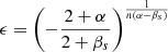 . We fixed the model’s high energy index following Ravasio et al. (2019). The low-energy index was instead assumed to be α = −2/3. The high-energy index is βs = −2.6, and the smoothness parameter is n = 2. The constant Cn normalises the spectral shape. We adopted the convention f(E = Ep) = 1, which sets
 ![Mathematical equation: $ C_{\text{n}} = \sqrt[n]{2} $](/articles/aa/full_html/2026/06/aa59597-26/aa59597-26-eq5.gif) . The temporal evolution of the light curve and peak energy follows the model in Ronchini et al. (2022), Ierardi et al. (2026).
. The temporal evolution of the light curve and peak energy follows the model in Ronchini et al. (2022), Ierardi et al. (2026).
From this evolving spectrum, we derived the key observables for comparison with the Fermi-GBM catalogue. The observed peak photon flux was calculated at the peak time τp and integrated over the GBM band between 50–300 keV (the most sensitive energy band of NaI detectors):
![Mathematical equation: $$ \begin{aligned} F_p(\theta _v, z) = \int _{E_1/(1+z)}^{E_2/(1+z)} \mathcal{N} (t = \tau _p, E, \theta _v, z)dE \quad \left[\frac{\text{ photons}}{\text{ cm}^{2} \text{ s} }\right] ,\end{aligned} $$](/articles/aa/full_html/2026/06/aa59597-26/aa59597-26-eq6.gif) (4)
(4)
where E1 = 50 keV and E2 = 300 keV. This quantity is additionally calculated on a 64 ms timescale to match the catalogue data. The bolometric energy light curve F(t) is given by integrating the energy spectrum at each time step:
![Mathematical equation: $$ \begin{aligned} F(t, \theta _v, z) = \int _0^\infty E \, \mathcal{N} (E, t, \theta _v, z) dE \quad \left[\frac{\text{ erg}}{\text{ cm}^{2} \text{ s} }\right] .\end{aligned} $$](/articles/aa/full_html/2026/06/aa59597-26/aa59597-26-eq7.gif) (5)
(5)
From this, we defined the cumulative fluence within the GBM band, S(t) = ∫0t∫E1/(1 + z)E2/(1 + z)E𝒩(E, t′,θv, z)dEdt′, from which the total fluence and the duration T90 were calculated.
2.2. Predicting the observed sGRB rate
We defined a fundamental parameter, fj, connecting the BNS merger population to the observed sGRB sample, given by the ratio between the intrinsic sGRB rate (NsGRB) and the BNS merger rate (NBNS):
 (6)
(6)
When fj ≤ 1, this quantity can be interpreted as the fraction of binary BNS mergers that are able to produce a successful relativistic jet, namely a jet that is able to break out from the post merger ejecta. In our framework we treat it as a free parameter inferred during the MCMC sampling, which ensures that all populations reproduce the same observed GRB rate. This approach allows fj to explore values greater than unity as a diagnostic tool to test the viability of the BNS population in reproducing the sGRB data. If the posterior distribution for fj lies predominantly above 1, it indicates that the BNS population model under consideration is insufficient to account for the observed sGRB rate.
We derive the predicted sGRB rate observed by Fermi-GBM by convolving the instrument’s duty cycle, the jet production efficiency, the source population properties, and the detector sensitivity. In the most general case the detection efficiency Φ depends on the redshift, the intrinsic engine parameters θp (e.g. tp or Ep), and the viewing angle θv. The predicted rate  is
is
 (7)
(7)
where ϵGBM ≈ 0.60 is the combined effective instrument efficiency and field-of-view (Burns et al. 2016), and dcos(θv) represents an isotropic distribution of viewing angles.
For the universal top-hat jet model (Sect. 2.3), the detection efficiency factorises because the emission is uniform within a cone of semi-aperture angle θc and negligible outside. We note that this sharp-edge approximation neglects the 1/Γ relativistic beaming spread of the emission pattern, which could allow detections slightly outside θc. However, for highly relativistic outflows (Γ ≫ 1), this contribution is subdominant and the factorised approximation remains valid for population-level counting. In this specific case, an observer detects a burst only if θv ≤ θc and the on-axis flux is above the threshold (Matsumoto et al. 2019). This allowed us to evaluate the integral of the geometric beaming independently:
 (8)
(8)
where ⟨fb⟩=(1 − cos θc) is the associated beaming factor. In our non-universal models (Sect. 2.3), where θc follows a distribution p(θc), the average beaming factor generalises to the probability that a random viewing angle is less than the core of a randomly sampled jet:
 (9)
(9)
where Θ is the Heaviside step function. By requiring  matches the observed rate
  , we could infer the necessary jet fraction fj for each BNS population model for different geometrical assumptions.
2.3. Jet structure models
The intrinsic energy described in Sec 2.1 is not emitted isotropically but is channelled into a relativistic jet. The geometry of relativistic jets in GRBs is poorly constrained through observations and serves as a major source of uncertainty in population studies. We investigate three distinct assumptions for the jet structure.
2.3.1. Universal structured jet
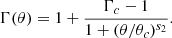
Our primary model assumes a universal, axisymmetric structured jet, strongly motivated by the afterglow of GRB 170817A. Here, the energy and bulk Lorentz factor decrease with angular distance θ from the jet’s core. We assumed angular profiles for the isotropic-equivalent kinetic energy and the bulk Lorentz factor given by
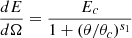 (10)
(10)
 (11)
(11)
Following Ronchini et al. (2022), we adopted fixed structural parameters consistent with the best-fit values for GRB 170817A (Ghirlanda et al. 2019): a core opening angle θc = 3.4°, an on-axis core Lorentz factor Γc = 500, and power law indices s1 = s2 = 4. The apparent properties depend on the viewing angle θv, with scaling factors for peak energy and flux calculated following the formalism of Ascenzi et al. (2020). In this framework, the MCMC samples seven free parameters: two for the energy distribution (power law index and cut-off k, E*), two for peak energy and spread(log10μE, σE), two for peak time and spread (log10μt, σt), and the jet fraction (fj).
2.3.2. Universal top-hat jet
To assess the impact of the assumed jet profile, we also analysed a simplified universal top-hat jet model. As mentioned above this model introduces a degeneracy between the jet fraction and the opening angle given by the efficiency fj(1 − cos(θc)) = const. This allowed us to determine geometries and jet fractions that are compatible with observed jet opening angles. In this framework, we do not use a temporal evolution of the light curve but instead sample the intrinsic peak luminosity L from a distribution analogous to Eq. (1). The observed peak flux is then calculated as Fp = L/(4πdL(z)2𝒦(Ep, z)), where 𝒦 is the k-correction factor (Salafia et al. 2023; Poolakkil et al. 2021). For this model, the MCMC samples six free parameters: two for luminosity power law index and cut-off (k, L*), two for peak energy and spread (log10μE, σE), the jet fraction (fj) and the core opening angle (θc).
2.3.3. Exploring non-universality
Finally, we relaxed the assumption of universality to test whether a diverse jet population significantly alters our constraints on BNS models. In this framework, we extended the top-hat jet model by allowing the core opening angle, θc, to vary across the population rather than being a single fixed value. We investigated two distinct scenarios for the population-wide distribution of θc, as illustrated in Fig. A.3. The first scenario is a flat model, where θc is drawn from a uniform distribution between a minimum of 1° and a variable upper bound,  . This model represents a scenario with no preferred physical scale for the opening angle, limited only by the maximum width of the jet geometry. The second scenario is a log-normal model, characterised by a median angle
  and a fixed shape parameter σlog10 = 0.5. This width is chosen to provide a realistic degree of diversity that covers approximately an order of magnitude in core angles, consistent with the heterogeneity observed in sGRB afterglow studies (Rouco Escorial et al. 2023).
To ensure physical consistency, both distributions produce minimum angles of θcmin = 1° and specifically for the log-normal case, we cut angles larger than θc ≥ 45°. Crucially, in these non-universal models, the isotropic equivalent peak luminosity L is sampled independently of θc. This implies that wider jets in our framework possess larger total jet energies (Etot ∝ Lθc2; Salafia et al. 2022), rather than assuming a constant energy reservoir that would imply L ∝ θc−2. We also explicitly tested this alternative scenario, confirming that it does not significantly alter our inferred posteriors (see Appendix B for details). In these non-universal models, the MCMC simultaneously samples the jet fraction fj and the specific distribution parameters (either  or
or  ). As in the universal top-hat model scenario, this approach allowed us to directly quantify the trade-off between the underlying BNS merger rate and the required jet geometry.
2.4. Fermi-GBM data
Historically, GRBs are classified into two populations: ‘short-hard’ and ‘long-soft’. This bimodality, first identified in Konus data (Mazets & Golenetskii 1981), was unambiguously established with the BATSE catalogue (Kouveliotou et al. 1993) through the separation of events in the duration-hardness plane.
To calibrate the BNS population with the sGRB observations, we selected sGRB data from the Fermi-GBM burst catalogue2 covering a time span of 16 years (July 2008 – May 2025; see Appendix C for more details). Our approach to select the sample is similar to that of Ghirlanda et al. (2016), Salafia et al. (2023), aiming to construct a well-defined dataset by applying specific cuts on GRB duration and peak flux. As a proxy for duration, we adopt T90, defined as the time interval containing 5% to 95% of the total measured fluence. Following established literature (e.g. Paciesas et al. 1999; Lien et al. 2016; von Kienlin et al. 2020), we applied the conventional threshold of T90 < 2 s to isolate the sGRB population. Although this threshold may include contamination from short-duration collapsars (single stars; Zhang et al. 2009; Bromberg et al. 2013), we verified that its impact on our population-level results is minimal. In fact, using a more restrictive T90 < 1 s cut, we find no significant changes in the distribution of GRB observables. Given the inherent difficulty in ensuring progenitor purity solely through duration (see e.g. Giudice et al. 2025), we retain the 2 s limit to maximise the sample size and minimise statistical uncertainty. To mitigate selection effects, we imposed a peak photon flux cut of Fplim = 4 ph cm−2 s−1 (measured on a 64 ms timescale in the 50–300 keV band). We further restricted our sample to events with observed spectral peak energies (Ep) between 50 keV and 10 MeV, corresponding to the GBM detection band (see Fig. C.1 for both cuts). The peak photon flux Fplim cut is chosen to ensure the cumulative peak flux distribution follows the N(> F)∝F−3/2 power law expected for a uniform distribution in Euclidean space (Ghirlanda et al. 2016; Ronchini et al. 2022). Notably, while the Fermi-GBM catalogue provides Ep values derived from Comptonised model fits, our framework employs an SBPL. As noted in the literature (e.g. Gruber et al. 2014), Comptonised fits return systematically higher Ep values (∼6% on average in our sample) compared to models with high-energy tails, such as the Band function or an SBPL. However, given the large individual statistical uncertainties on Ep, this minor systematic offset is well within the intrinsic scatter of the population, and this discrepancy does not introduce significant bias (see Sect. 2.1 for a more thorough discussion). After the cut in peak flux, our sample contains 310 sGRBs. This corresponds to an observed rate of  . This rate is less than the one used in Ronchini et al. (2022), as a lower value for Fplim (0.5) was used in that work. After applying the quality cut on the peak energy, we are left with 221 events. For each of these events, we retrieved the catalogued values for the fluence in the 50–300 keV band, T90, peak flux in the 50–300 keV band and peak energy. We adopt this band, since the T90 of each GRB is computed only in that band in the Fermi-GBM catalogue. We highlight that even if we impose a cut on the measured peak energy to ensure a good fit quality, that cut is relative only to the GRBs considered for the comparison between the predicted and observed distributions. However, in estimating the true GBM detection rate, we impose no quality cuts and consider all events that triggered the detector, regardless of data quality.
2.5. Theoretical populations of BNS mergers
In this work, we use a comprehensive set of 16 binary population synthesis models from Iorio et al. (2023). These models explore the large parameter space of stellar and binary evolution uncertainties. Here, we briefly recap how the merger rate density and its redshift evolution are obtained and highlight the assumptions (see Sects. 2.5.1 and 2.5.2) that have the most significant impact on the merger rate density.
The models are generated using the SEVN code, which evolves a total of ∼109 binary systems across 15 metallicity bins spanning the range Z ∈ [10−4, 3 × 10⁻²]. The primary masses, mZAMS,1, are drawn from a Kroupa initial mass function (IMF; Kroupa 2001) over the range [5, 150] M⊙, with a minimum secondary mass of mZAMS,2 = 2.2 M⊙. We used the semi-analytic code COSMOℛATE (Santoliquido et al. 2020, 2021) to compute the cosmic merger rates from the merged binaries simulated with SEVN (Spera et al. 2019; Mapelli et al. 2020). The source frame merger rate density, ℛ(z), was computed by convolving the delay-time distribution of the binaries with the cosmic star-formation history:
 (12)
(12)
where t(z) is the look-back time at redshift z. The term ℱ(z′,z, Z) is defined as
 (13)
(13)
where Mpop(Z) is the total initial mass of the simulated stellar population, normalised to the full IMF mass range. The term  represents the rate of binary compact object mergers forming from stars with initial metallicity Z at redshift z and merging at redshift z′ extracted from the SEVN catalogues. We adopted the analytical fit for the star formation rate density, ψ(z), from Madau & Fragos (2017):
![Mathematical equation: $$ \begin{aligned} \psi (z) = a \frac{(1 + z)^b}{1 + [(1 + z)/c]^d} \, [M_{\odot } \, \text{ yr}^{-1} \, \text{ Mpc}^{-3}], \end{aligned} $$](/articles/aa/full_html/2026/06/aa59597-26/aa59597-26-eq25.gif) (14)
(14)
with parameters a = 0.01, b = 2.6, c = 3.2, and d = 6.2. The metallicity distribution p(Z ∣ z) was assumed to follow a log-normal distribution:
![Mathematical equation: $$ \begin{aligned} p(Z \mid z) = \frac{1}{\sqrt{2\pi \sigma _Z^2}} \exp \left\{ -\frac{[\log (Z/Z_{\odot }) - \langle \log Z(z)/Z_{\odot } \rangle ]^2}{2\sigma _Z^2} \right\} , \end{aligned} $$](/articles/aa/full_html/2026/06/aa59597-26/aa59597-26-eq26.gif) (15)
(15)
with σZ = 0.1. From the merger rate density, we defined two key quantities for our analysis, the local BNS merger rate density, RBNS(0)≡ℛ(z = 0), and the total integrated rate, Λ, defined as
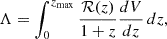 (16)
(16)
where  is the differential co-moving volume.
In our analysis, we assumed the Fiducial population (Model F, αCE = 1, σz = 1) from Iorio et al. (2023) as our baseline. This model yields a local merger rate density of RBNS(0) = 112 Gpc−3 yr−1, which lies near the centre of the 90% credible interval reported in the GWTC-4 catalogue (The LIGO Scientific Collaboration 2025). A summary of all analysed BNS merger populations is provided in Appendix D.
2.5.1. Common envelope
The common envelope (CE) phase is a critical, yet highly uncertain, stage in binary evolution (Webbink 1984; Livio & Soker 1988) and can change predicted BNS merger rates by orders of magnitude (Ivanova et al. 2013; Broekgaarden et al. 2022; Santoliquido et al. 2021; Mandel et al. 2020). In the CE phase, both stars orbit within a shared and extended envelope. Drag forces remove orbital energy and angular momentum, shrinking the orbit. If the orbital energy deposited into the envelope is sufficient to unbind it, the envelope is ejected, leaving behind a tighter post-CE binary. Otherwise, the stars coalesce. The CE ejection efficiency, αCE, sets how effectively orbital energy unbinds the envelope. Low αCE (e.g. 0.5 and 1) requires closer inspirals to eject the envelope, increasing premature mergers during CE while surviving binaries have tighter orbits and shorter GW-driven delay times. Iorio et al. (2023) finds that for αCE ≤ 1, premature coalescences suppress BNS formation overall. High αCE (e.g. 3 and 5) favours CE survival at wider separations. Across models, varying αCE shifts the local BNS merger rate density from fewer than one to over 300 Gpc−3 yr−1 (Figs. 19, 20, 22 in Iorio et al. 2023), confirming αCE as the dominant parameter in determining the theoretical BNS merger rate (Santoliquido et al. 2021). Within this work we consider the values αCE = 0.5, 1, 3, 5.
2.5.2. Natal kicks, mass transfer stability, and other assumptions
The velocity kicks imparted to neutron stars at birth are important for binary evolution. Models drawing kicks from a Maxwellian distribution (see Hobbs et al. 2005) with dispersion σ = 150 km/s (model K150) yield higher BNS survival and merger rates than models with σ = 265 km/s (Kσ265), where disruptions are more frequent.
The criteria that determine whether mass transfer from one star to another is stable or instead initiates a CE phase can also alter BNS formation channels and rates. The fiducial model assumes mass transfer is always stable for main sequence and Hertzsprung gap donors. The QCBSE model instead adopts the standard stability criteria from Hurley et al. (2002), widely used in codes like MOBSE (Giacobbo & Mapelli 2018). The QCBB model goes further, assuming mass transfer is also always stable for pure-Helium star donors, which allows for stable mass transfer from pure-Helium stars in scenarios that might otherwise be considered unstable and thus enhances the BNS merger rate by providing an additional formation channel, following Mandel et al. (2020).
Several other physical parameters were tested by Iorio et al. (2023), but they were found to have a comparatively minor direct impact on the overall BNS merger rates. These include variations in Roche-lobe overflow accretion efficiency (model RBSE), the specific supernova engine model (SND), the pair-instability supernova model (F19), and the treatment of tides (NT, NTC). While these factors can influence other aspects of compact binary populations or specific BNS properties, their effect on the total BNS merger numbers is secondary to the parameters discussed above.
We analysed sixteen population synthesis models from Iorio et al. (2023). For each, we considered four values of αCE resulting in a total of 64 BNS merger populations.
2.6. Analysis framework
From each BNS population, we generated a corresponding synthetic sGRB population calibrated to reproduce the Fermi-GBM observations. We employ a hierarchical Bayesian analysis to infer the properties of the sGRB population from the observed data. For each of the three jet structure models described in Sect. 2.3, we defined a posterior probability distribution for the model’s free parameters, θ. We then sampled this posterior using a MCMC algorithm, implemented with the EMCEE package (Foreman-Mackey et al. 2013). The specific set of parameters θ and their priors are detailed below for each model.
2.6.1. Universal structured jet model
This model requires a time-evolving light curve and spectrum. The MCMC samples seven free parameters, θ = {k, E*, μE, σE, μt, σt, fj}. Their descriptions and prior ranges are given in Table 1.
Free parameters and prior distributions for the sGRB emission models.
2.6.2. Universal top-hat jet model
In the universal top-hat jet model, the core half-opening angle θc is assumed to be the same for all the sGRBs. The abundance of observed sGRB is given by the efficiency, ϵ = fj(1 − cos θc). This approach allowed us to quantify how specific geometric assumptions impact the required BNS abundance (fj). This model does not include time evolution and samples the intrinsic peak luminosity directly. It has six free parameters, θ = {k, L*, μE, σE, θc, fj}. While we kept the same prior of fj as before, we added a flat prior θc ∈ [1° ,25° ]. This choice is motivated by observational constraints on sGRB beaming. Population studies of late-time afterglows find a median opening angle of ⟨θc⟩≈6° with a tail to wider jets, including measurements and lower limits of θc ≥ 10° in ≈30 % of the sample in Rouco Escorial et al. (2023). Early X-ray afterglow analyses further indicate that most sGRBs are viewed within or very near their jet opening angle, consistent with compact cores and disfavouring very large core angles (O’Connor et al. 2024). Thus, θc ≤ 25° is conservative and comfortably includes most of the observed wide core tail without truncating plausible values, while avoiding prior support for unrealistically large cores. All parameters and their priors are detailed in Table 1.
2.6.3. Non-universal top-hat jet models
The non-universal models expand upon the structured jet and universal top-hat jet frameworks by allowing the core opening angle, θc, to vary on an event-by-event basis, according to an underlying population distribution. This approach introduces an additional parameter, Pθ, to the MCMC sampling, which describes the characteristic scale of the core geometry. The sampled parameter set for these models is θ = {k, L*, μE, σE, θc, fj, Pθ}, as detailed in Table 1. For the Flat model, Pθ represents the upper bound θcmax. In this scenario, the opening angle was sampled from 𝒰(1° ,θcmax), effectively testing a population with no preferred scale up to a maximum cut-off (θcmax < 25° ). For the Log-Normal model, the parameter Pθ corresponds to the median angle θcmed. As noted in the previous section, we fixed the dispersion to σlog10 = 0.5 to ensure the population spans roughly one order of magnitude in jet core angle width. To maintain physical consistency and avoid negative or non-physically large angles, the distribution was truncated and renormalised to the range [1° ,45° ]. In both cases, the simultaneous inference of the jet fraction fj and the geometric hyperparameter allowed us to study the degeneracy between the BNS merger rate and the intrinsic beaming of the sGRB population. We highlight that although the MAGGPY framework is designed to allow users to define and test arbitrary jet structures, the present analysis focuses exclusively on the three models described above, as they provide a representative coverage of the geometric uncertainties most relevant to the sGRB population.
2.6.4. Likelihood
For each set θ drawn from the priors, we generated a synthetic catalogue of sGRBs. From a population of BNS mergers with redshifts and viewing angles, the sGRB/BNS ratio fj (see Eq. (6)) determines the number of successful GRBs. We then drew the intrinsic properties for each event and applied the corresponding jet model to derive the observable quantities. For the structured jet model we derived four key observables for comparison with the Fermi-GBM data: fluence (Si), peak flux (Fp, 64, i), peak energy (Ep, i), and duration (T90, i). For the top-hat models, which lacks a temporal profile, the comparison was performed using only the peak flux and peak energy. The final set of selected bursts, Ndet, sim, are those that satisfy the selection criteria from our observational sample.
The comparison between simulated catalogue and real Fermi-GBM data is based on two components: the observable distribution shape and the event rate. To compare shapes, we used the two-sample Cramér-von Mises (CvM) test, which integrates the squared difference between the Empirical Cumulative Distribution Functions (ECDFs) of the simulated and observed data. This integral approach makes the test sensitive to discrepancies across the entire distribution, rather than a single local maximum. The choice of CvM over the Kolmogorov-Smirnov (KS) statistic used in previous works (Ronchini et al. 2022) is motivated by its superior stability and higher statistical power in Monte Carlo sampling (Stephens 1974). While both statistics are consistent and converge to the same limit, the CvM statistic exhibits lower variance across stochastic simulations (D’Agostino & Stephens 1986). This provides a p-value, pCvM, X, for each observable X. To constrain the rate, we used a Poisson likelihood, PPoisson = Poisson(Ndet, sim|μexp), where μexp is the expected number of detections. Given the complexity of the detector effects, constructing a direct analytical likelihood is not feasible. Combining these metrics, we obtained the likelihood
 (17)
(17)
where the sum over X includes the relevant observables. The MCMC maximises this function to find the sets θ that best reproduce the observed sGRB population. Details regarding the convergence of our chains and posterior predictive checks are provided in Appendix E.
3. Results
Here, we present the outcomes of our analysis, performed independently for each of the 64 BNS population synthesis models. By comparing the predictions derived under different assumptions for the sGRB jet structure, we assess the physical viability of each BNS model and the robustness of our conclusions. The primary diagnostic is the posterior distribution of the jet fraction fj, which is constrained by the requirement that the model reproduces the observed Fermi-GBM sGRB population. By allowing fj > 1, we derived a quantitative metric for model viability, which is the degree to which a model fails to produce enough progenitors to match the Fermi-GBM rate.
3.1. Structured jet population
Applying our analysis to all 64 BNS population synthesis models and assuming a structured jet as described in Sect. 2.3, we obtained the posterior distributions of the jet fraction, fj, shown in Fig. 1. These distributions form the basis for evaluating the physical viability of each population.
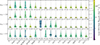 |
Fig. 1. One-dimensional marginalised posterior distributions of the jet fraction fj for each considered BNS population model, assuming a universal jet structure calibrated to GRB170817A. Black lines mark medians; labels also provide the 90% C.I. values. Axes show models (x-axis) and αCE (y-axis). The colours indicate the local merger rate. |
A wide range of fj posterior distributions is observed, reflecting the significant variation in predicted merger rates across the models spanning orders of magnitude. Models predicting intrinsically high merger rates are compatible with relatively smaller jet fractions. Typically, higher merger rates correspond to larger αCE. However, for several models, a trend is observed in which αCE = 5 yields lower merger rates than αCE = 3. This behaviour is primarily due to the higher efficiency of CE ejection, which leaves the binary system at a wider separation after the CE phase, thereby requiring a longer time to merge. Conversely, for models predicting low intrinsic merger rates (e.g. those with low αCE or high kicks like the model K265) the posterior distributions of fj are widely spread above the physical threshold of unity. This suggests a scenario for these models where the predicted number of BNS mergers is insufficient to explain the sGRB observations. As detailed in Appendix F, we allowed fj > 1 rather than enforcing a strict physical boundary because it provides a quantifiable metric of the missing mergers required by low-rate models, enabling a clearer distinction between marginal and significant model tensions that would otherwise be obscured by saturation at the prior limit. To better understand the relationship between jet fraction and BNS merger rate, we plot the median posterior value of fj against the local BNS merger, RBNS(0), and the total event rate obtained by integrating over redshift, Λ, for each population synthesis model in Fig. 2 (top row). Here, the anti-correlation between rate and jet fraction is more clearly visible. This correlation exhibits scatter, which is more pronounced when plotting against the local merger rate than the total integrated rate. This scatter arises from models predicting different redshift evolutions, which alters the total number of detectable events in a way that is not captured by the local rate alone.
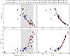 |
Fig. 2. Jet fraction statistics for the universal structured jet model assuming the GW170817/GRB170817A structure. Top row: Median jet fraction fj versus the predicted local BNS merger rate density RBNS(0) (left) and total integrated rate Λ (right). Bottom row: Quantile of the posterior distribution of fj at fj = 1 as a function of local BNS rate density (left) and total integrated rate Λ (right). Symbols are coloured according to the αCE parameter, and each symbol denotes a different population. The shaded vertical region indicates the 90% credible interval for the BNS merger rate from GWTC-4 (The LIGO Scientific Collaboration 2025). The cited fractions from the works of Ronchini et al. (2022) and Loffredo et al. (2025) are given as R22 and L25 for comparison. |
We also quantified the fraction of the posterior of fj that lies in the non-physical region by plotting the quantile evaluated at the boundary fj = 1, i.e. P(fj ≤ 1), shown in the bottom row of Fig. 2. Throughout this work, we defined a BNS population as physical if the median of its jet fraction posterior satisfies fj ≤ 1 (equivalent to requiring P(fj ≤ 1)≥0.5). These can be considered as the preferred models, i.e. those for which BNS abundance is enough to reconcile with sGRB observations. Notably, we find that models predicting RBNS(0) ≲ 100 Gpc−3 yr−1 exhibit a progressive shift of the jet fraction fj posterior above unity. This indicates that under the assumption that BNS mergers are the sole progenitors of sGRBs, explaining the observations would require either a non-physical scenario in which more than one GRB is produced per BNS merger or the presence of additional progenitor channels.
This finding provides a powerful, independent constraint when compared with GW observations. The shaded vertical region in Fig. 2 shows the 90% credible interval for the BNS merger rate from GWTC-4 (The LIGO Scientific Collaboration 2023). While many of the analysed models fall within this broad interval, our sGRB analysis effectively establishes a multi-messenger viability window for the BNS mergers as the progenitors of the entire sGRB population.
We can define a conservative lower bound at RBNS(0) ≲ 50 Gpc−3 yr−1 for which the majority of the found posterior distribution is within non-physical bounds and for which the MCMC analysis indicates that at least a factor of 2–3 larger BNS merger rate would be required to reproduce the observed sGRB rate. Conversely, the GWTC-4 bounds RBNS(0) ≤ 250 Gpc−3 yr−1 give an upper limit on the BNS local rate.
We note that the range for the BNS local rate from GWTC-4 was obtained by adding only a small portion of the O4 run (almost the first 7 months) to the first three LVK observing runs, and that, to date (Feb 2026), no significant BNS candidate has been released in low-latency in the subsequent one year and half of the O4 run. If the final analysis of O4 data and future GW observations push the allowed parameter space towards BNS merger rates lower than the floor implied by our sGRB constraints, it would become increasingly difficult to account for the full sGRB population with BNS mergers alone. Such a scenario would strengthen the case for a significant contribution from alternative progenitors, such as neutron star-black hole (NSHB) mergers, or that different geometric hypotheses including much wider jet cores are necessary. We therefore arrive to the conclusion that under the assumption of a universal GW170817-like jet structure for the sGRB population and that BNS mergers constitute the sole dominant progenitor channel, BNS populations with local merger rates RBNS(0) ≲ 50 Gpc−3 yr−1 are difficult to reconcile with sGRB observations.
3.2. Universal top-hat jet
We repeat the analysis using a simplified universal top-hat model. This model constrains the overall efficiency ϵ = fj(1 − cos(θc)), which combines the jet fraction and the beaming angle. This allowed us to test various values of jet core aperture. In Appendix E we show the posterior distributions for the fiducial BNS population (Fig. E.3). The corresponding median values and confidence intervals are provided in the right-hand columns of Table E.1. We find that the overall efficiency ϵ must be low to reproduce the observed data. The posterior distributions of the parameters k, μE, and σE closely match those found for the structured model (see Table E.1 and Fig. E.2). The L* posterior is consistent with findings from other works on the GRB luminosity distribution, such as Wanderman & Piran (2015, ∼1051 erg/s).
The results for the 64 population models are summarised in Fig. 3. Although the sampler explores fj and θc separately, we visualise the efficiency ϵ as the observed rate is directly proportional to this parameter. As expected, models with lower BNS rates require an overall higher efficiency ϵ to reproduce GRB observables. Owing to the degeneracy between the jet fraction and the jet aperture, this implies that such populations would require jet fractions exceeding unity or unrealistically large jet cores. To visualise this effect and to enable a direct comparison with our structured jet model, we condition the two-dimensional posterior of P(fj, θc) on three fixed values of the opening angle (θc= 5°,10°, and 20°). Figure 4 demonstrates that for both narrow and wide jet assumptions, BNS models with very low intrinsic merger rates yield fj posteriors that extend significantly above unity.
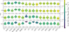 |
Fig. 3. Same as Fig. 1 but with the one-dimensional marginalised distributions of ϵ = fj(1 − cos(θc)) for all the BNS populations, considering the universal top-hat jet model. For clarity log(ϵ) is shown. |
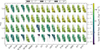 |
Fig. 4. Same as Fig. 1 but assuming a universal top-hat jet with three different opening angles, θc = 5°, 10°, and 20°. These posteriors were obtained from the conditioned distribution P(fj ∣ θc) (see Fig. 3). The model LK with αCE = 0.5 does not have any samples below fj ≤ 10 for θc = 5°. |
As in the structured jet case, for each assumed value of the opening angle θc, we computed the fraction of the posterior that is physical (i.e. P(fj ≤ 1 ∣ θc)) to provide a more direct assessment of which models can reasonably reproduce the observed sGRB rates. A model is considered physical if the median of its jet fraction distribution is ≤1, which corresponds to P(fj ≤ 1)≥0.5. The quantiles associated with the 3 analysed geometries are shown in Fig. 5, where we observe that for lower opening angles (θc ≈ 5°), models with local rates RBNS(0) ≲ 50 Gpc−3 yr−1 have almost their entire posterior distribution spread above fj > 1, in agreement with what found in the universal structured jet scenario. To reconcile these low-rate models with observations, significantly larger opening angles (θc ≳ 10° −20°) are required. This creates tension with observations of sGRB jet breaks, suggesting a low median opening angle ⟨θc⟩≈6° (Rouco Escorial et al. 2023). While the top-hat model confirms that the geometric degeneracy allows low rates to be compensated for by wide jets, the tight geometry, inferred for GW170817 and applied to the entire BNS population, implies that BNS merger rates must be relatively high to remain physically viable as the sole progenitors of sGRBs.
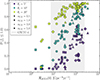 |
Fig. 5. Same as the bottom row of Fig. 2 but assuming a universal top-hat with three different aperture angles. |
3.3. Non-universality
We further relaxed the assumption of universality by allowing the jet core angle θc in our top-hat jet model to be drawn from a population-wide distribution (uniform and log-normal as defined in Sect. 2.3) for θc, treating the distribution’s parameters as additional free parameters in the analysis. The posterior distributions from this analysis are shown in Fig. 6 for our fiducial population. We only show the posteriors for the geometry and jet-fraction as the other parameters are almost identical to Fig. E.3. Both models exhibit a similar degeneracy between the parameters Pθ and fj. One immediate result is that the log-normal model’s extended tail allows a substantial fraction of the fj posterior to lie below unity, even for small sampled θcmed angles. In contrast, the flat model places a large portion of fj posterior above unity for almost all small θcmax angles. To systematically compare these non-universal results with the universal top-hat model and observational constraints, we introduce a unified geometric metric described below.
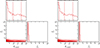 |
Fig. 6. Two-dimensional marginal posterior distribution P(fj, θc, max) for the non-universal flat model (left) and P(fj,θc,med) for the non-universal log-normal model (right) using our fiducial BNS population. The remaining parameters remain consistent with the results of a universal top-hat (see Fig. E.3). |
3.4. Narrowest geometry
To benchmark all our BNS models against observations, regardless of the assumed top-hat jet model, we quantify here the trade-off between the intrinsic merger rate and the jet geometry. The observed sGRB rate depends on the GRB population beaming factor ⟨fb⟩ and jet fraction fj such that for a fixed population model (see Sect. 2.2), the predicted detection rate scales as

where Pθ represents the parameters of the jet opening angle distribution (e.g. θc for the universal top-hat, θcmax for the flat model, or θcmed for the log-normal model). Because the observed rate is fixed by Fermi-GBM data, a strict degeneracy exists as fj × ⟨fb⟩=ϵ, where ϵ is a constant specific to each BNS population. If we impose that fj takes only physical values (median fj ≤ 1), there exists a minimum beaming factor ⟨fb⟩min required to reproduce the observed event rate. We translate this into a minimum characteristic opening angle, θ*, defined as the narrowest population median angle  that satisfies the physical condition
 (18)
(18)
We calculated θ* for three distinct distribution geometries:
-
Universal top-hat:P(θc)∼δ(θ − θc) distribution where ⟨fb⟩ = 1 − cos θc and the median
 .
. -
Flat distribution:P(θc)∼𝒰(θcmin, θcmax), where
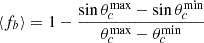
and with a population median
 .
. -
Log-normal distribution: Defined by a median θcmed and shape σ, where

and with
 .
.
For each posterior sample (fj, Pθ) we can calculate ϵ = fj × ⟨fb⟩ and derive the median ⟨ϵ⟩. Numerically we solved ⟨fb(Pθ)⟩ − ⟨ϵ⟩ = 0. From the minimum Pθ we define θ* from the associated population median  . An example on how θ* is recovered for the universal top-hat model in the case of our fiducial population is shown in Fig. G.1. The figure shows how the fj − θc posterior follows the predicted line at ⟨ϵ⟩=⟨fj⟩(1 − cos(θc)) = const. We then calculated the θ* value for each of the 64 populations across all three geometric assumptions as shown in Fig. 7 and compared these values with the jet opening angles inferred from sGRB afterglow observations (Rouco Escorial et al. 2023). Under the universal top-hat assumption (Fig. 7, top left panel), BNS population models predicting lower intrinsic merger rates require significantly wider θ* values to compensate for the lower event count. Models with RBNS(0) ≈ 100 Gpc−3 yr−1 yield θ* values close to the observed median of ⟨θc⟩≈6° reported in Rouco Escorial et al. (2023). As the authors of Rouco Escorial et al. (2023) mention, we are aware that estimates of ⟨θc⟩ might be biased by selection effects (see the many lower limits set therein) we nonetheless use it as a reference point, while showing the trend of opening angles compared to local rates. In contrast, lower-rate models are forced to assume geometries significantly wider than typical observed values. This trend persists for the non-universal Flat model (Fig. 7, top right panel). As merger rates decrease, the required population median θc moves beyond the 1σ upper bound of afterglow observations. For some populations, the local rate is so low that no numerical value of θ* satisfies the condition of Eq. (18), since the required value would lie above the maximum value of the prior θcmax, effectively excluding these populations as viable progenitors under this assumption. To remain compatible with the narrow geometries inferred from X-ray observations (θc ≤ 10°), the underlying BNS population must possess a local rate RBNS(0) ≥ 50 Gpc−3 yr−1. The non-universal Log-Normal model (Fig. 7, bottom left panel) offers more flexibility due to its extended tail, allowing lower-rate BNS models to have a median fj ≤ 1 by populating the distribution with wide-angle jets. However, this comes at the cost of physical plausibility. As shown in the bottom right panel of Fig. 7, for models with RBNS(0) ≲ 20 Gpc−3 yr−1, more than ∼10% of the sGRB population would require core angles θc ≥ 15° to maintain a physical jet fraction. This result, under the log-normal assumption, highlights the presence of a subgroup of BNS populations that, in order to have a fj distribution with a median below one, require a distribution of aperture angles containing a substantial fraction that stands in tension with current observational constraints on sGRB jet collimation.
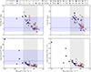 |
Fig. 7. Minimum characteristic jet opening angle, θ*, required to keep the median jet fraction physical (median fj ≤ 1) as a function of the local BNS merger rate RBNS(0) for the universal top-hat (top left), non-universal flat (top right), and non-universal log-normal (bottom left). Each symbol denotes a different population. The horizontal dashed line and shaded region indicate the median and 90% credible interval of the aperture angle distribution derived from Rouco Escorial et al. (2023). Bottom right panel: Fraction of the population with wide jets (θc > 15°) for the log-normal model. The vertical grey band represents the GWTC-4 90% C.I. for the BNS merger rate. The plots do not display all 64 analysed populations, as some require θ* larger than the prior upper limit of 25°. See Table H.1 for a comprehensive list of all the populations. |
A comprehensive summary of the physical viability and geometric consistency for all 64 BNS population models across the four analysed jet scenarios is provided in Table H.1. The specific criteria used to evaluate these models, including the treatment of non-physical jet fractions and observational tensions, are further detailed in Appendix H.
4. Discussion
Our analysis demonstrates that sGRB observations provide powerful independent constraints on BNS models. By calibrating the sGRB/BNS ratio (fj) to the observed Fermi-GBM rate, we identify a clear tension between low-rate progenitor models and electromagnetic observations in terms of sGRB local rate, its evolution, and the inferred jet opening angle. In the following, we summarise and discuss the results obtained for the various jet models considered.
-
Under the assumption of a universal structured jet consistent with GW170817/GRB170817A, BNS population models predicting RBNS(0) ≲ 50 Gpc−3 yr−1 are effectively ruled out, because the number of BNS mergers is insufficient to account for the full population of observed sGRBs (the inferred median is fj > 1). BNS population models with a local merger rate of RBNS(0) ≈ 100 Gpc−3 yr−1, consistent with the current GWTC-4 constraints, are able to reproduce the observed sGRB population provided that the jet fractions are fj ≈ 0.7 − 0.8.
-
The use of a universal top-hat model allowed us to quantify the degeneracy between merger rates and jet geometry. We find that, in order to maintain physically plausible jet fractions, low-rate models are forced to adopt opening angles θc ≳ 15° −20°, which are in significant tension with the median value of ≳6°, inferred from the observation of jet break in afterglow light curves of sGRBs. In contrast, populations with RBNS(0) ≈ 100 Gpc−3 yr−1 lie remarkably close to the observed median, allowing for physically plausible jet fractions without requiring wide-angle geometries.
-
This conclusion remains robust when relaxing the assumption of universality by adopting a flat or log-normal distributions for the jet core opening angle. These non-universal jet models show that low-rate BNS population scenarios can reproduce the observed sGRB counts by forcing the jet opening angle distribution towards systematically wider jets. For instance, a low–merger-rate BNS population assuming a log-normal jet model requires more than 10-20% of the systems to have core angles θc > 15°. Such a requirement is not supported by the scarcity of wide-jet observations in sGRB catalogues.
Our finding of physically viable BNS populations capable of reproducing sGRB observations which tend to favour jet-fraction close to unity, is in good agreement with other recent population studies that have taken different approaches to the problem, such as the work by Salafia et al. (2023), which utilised a more granular treatment of detector efficiency and inferred local sGRB rates above 100 Gpc−3 yr−1, implying a high jet production efficiency. Constraining the jet fraction, has physical implications beyond binary evolution. The ability of a BNS merger remnant to launch a relativistic jet is thought to depend critically on the nature of the central engine (Ciolfi 2020), which is in turn governed by the binary’s total mass and the neutron star equation of state (EoS; e.g. Giacomazzo & Perna 2013; Ruiz et al. 2021). Our finding of high jet production efficiency disfavours scenarios where prompt collapse to a black hole systematically suppresses jet production or alternatively implies that even prompt-collapse systems can launch jets efficiently.
We emphasise that the results of our analysis, shown in the different figures, provide a framework for assessing the validity of BNS merger population models in light of the progressively improving observational constraints expected from GW observations and complementary electromagnetic measurements of sGRBs. However, we can already conclude that if future GW observations continue to push the BNS rate towards the lower rates, the discrepancy between the required wide jets and the observed narrow ones (Rouco Escorial et al. 2023) would suggest that either BNS mergers are not the sole progenitors of sGRBs or our understanding of jet observational biases is incomplete.
4.1. Intrinsic local sGRB rate densities
Using our theoretical and statistical framework, we examine the intrinsic local sGRB rate densities (regardless of the viewing angles) inferred from our models and compare them with values reported in the literature. For each BNS population, we define the rate of successfully launched sGRB jets as RsGRB = RBNS(0)×fj, where RBNS(0) is the local BNS merger rate predicted by population synthesis and fj is the jet fraction inferred via our analysis. This value represents the all-sky intrinsic local density of sGRB jets produced per year. The resulting distributions for the intrinsic local sGRB rate density, assuming our universal structured jet model, are presented in Fig. 8 (left panel). We contextualise these results by comparing them to recent derived constraints. Salafia et al. (2023, S23) estimated rates using a flux-limited sample similar to ours, finding  , while Rouco Escorial et al. (2023, RE23) report a rate
  (
( for the mock sGRB sample) based on the observed local rate and the jet opening angles determined from the afterglows. We observe that our inferred rates for physically viable populations (specifically those where their median is fj ≤ 1) generally sit at the lower end or below the median estimates of S23 and RE23. The higher intrinsic local sGRB rates favoured by other studies would increase the tension with the hypothesis that BNS mergers are the sole progenitors of sGRBs, as they would require non-physical jet fractions (median fj > 1). The local sGRB rates are inferred from sGRBs observed out to high redshift, and this tension may also indicate that the redshift distributions assumed in those studies do not accurately reflect the redshift evolution of BNS mergers.
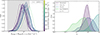 |
Fig. 8. Left: Inferred intrinsic local sGRB rate RsGRB for all the BNS population models that allow physical jet fractions (with median fj ≤ 1), under the assumption of a universal structured jet. Right: Comparison of the inferred fj posterior distributions for the fiducial BNS population across the four analysed jet structures: universal structured, universal top-hat, non-universal flat, and non-universal log-normal. |
The sensitivity of our conclusions to the assumed jet geometry is illustrated in Fig. 8 (right panel), where we show the fj posterior distributions for our fiducial BNS population across the four analysed jet models. While the universal structured and top-hat models yield comparable constraints, the non-universal models diverge significantly based on the shape of their opening angle distribution. Notably, the log-normal model yields a posterior distribution located almost entirely below fj = 1. This demonstrates that a geometric distribution with a long tail towards wide opening angles can effectively alleviate the tension for lower-rate models. The presence of a sub-population of wide jets increases the average beaming factor, thereby reducing the total number of progenitors required to match the observed Fermi-GBM rate. Conversely, the flat model results in a posterior centred well above unity, indicating a much stronger tension. This confirms that for most angles the MCMC is unable to infer physical jet fractions, even BNS models with moderate merger rates may fail to reproduce the observed event counts without non-physical efficiencies. Since RsGRB ∝ fj, Fig. 8 (right panel) can be used to estimate what is the impact of the assumption of jet structure on the inferred sGRB local rate.
4.2. Delay-time distribution of BNS populations
Here, we analyse the distributions of delay times between the formation and the merger for BNSs, to compare them with the recent findings of Pracchia & Salafia (2026) in Fig. 9. The delay times are calculated starting from the catalogues of Iorio et al. (2023) and using the code COSMOℛATE (see Sect. 2.5). While early studies suggested long delay times (a few gigayears) for sGRBs, Pracchia & Salafia (2026) demonstrated that correcting for selection effects in flux-incomplete samples leads to significantly shorter delays, with average values ⟨τd⟩≈10 − 800 Myr. Figure 9 show the average time delay corresponding to each of our BNS populations. All models but one (QCBB with αCE = 1) exhibit short delay times (⟨τd⟩< 1 Gyr) in agreement with the 90% credible intervals reported by Pracchia & Salafia (2026). We also clarify how our time delay average values are derived directly from the BNS population synthesis catalogues and are independent of our sGRB inference. In Appendix I we also show the redshift evolution of the average delay time.
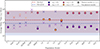 |
Fig. 9. Average delay time ⟨τd⟩ for each of the 64 BNS population models compared to the median and 90% credible intervals inferred in Pracchia & Salafia (2026). The blue and red lines and ranges correspond to two models by Pracchia & Salafia (2026): a quasi-universal structured jet model and an empirical luminosity function model, respectively. To highlight the relationship between delay times and model viability, we mark with circles the populations that yield a physical jet fraction (with median fj ≤ 1) under the universal structured jet assumption and use crosses for those that are considered non-physical. |
4.3. Caveats
4.3.1. Progenitor purity.
A central goal of our analysis is to test the hypothesis that BNS mergers are sufficient to explain the entire observed sGRB population. We use the inferred jet fraction as a diagnostic for this test. Any scenario that requires more SGRBs than BNS progenitors (fj > 1) is interpreted as evidence against the BNS-unique progenitor hypothesis, implying that the BNS population under consideration is not numerous enough to account for the observed sGRB rate. This could suggest a contribution from an alternative channel, such as NSBH mergers (Colombo et al. 2025). However, the association between NSBH mergers and sGRBs has not yet been firmly established observationally and remains more difficult to quantify. The outcome of NSBH mergers is highly model-dependent and sensitive to the mass ratio, the black hole spin, and the neutron star EoS (Foucart 2012; Krüger & Foucart 2020). Numerical simulations and analytical fits suggest that only a subset of the NSBH population, specifically those with high BH spins and/or low mass ratios, yields enough remnant mass to power a jet. These stringent requirements often result in a majority of systems failing to launch a jet (Sarin et al. 2022; Clarke et al. 2025; Biscoveanu et al. 2023), implying smaller fj ≪ 1 for the NSBH population. Regarding the population abundance, while some synthesis models predict NSBH rates to be lower than BNS rates by an order of magnitude (Iorio et al. 2023), current observational constraints from GWTC-4 indicate that the two rates may be comparable. Specifically, GWTC-4 reports a BNS merger rate of 7.6–250 Gpc−3 yr−1 (90% C.I) and an NSBH merger rate of 9.1–84 Gpc−3 yr−1. Despite this, because only a small fraction of the NSBH population is expected to produce significant ejected mass and a subsequent jet, we assume that their contribution would not significantly alter the inferred jet fractions presented in this work especially for comparatively higher rate models. We also acknowledge that the traditional classification distinguishing long and short GRBs has blurred by recent discoveries of long-duration bursts with kilonova counterparts, such as GRB 211211A and GRB 230307A (Rastinejad et al. 2022; Levan et al. 2023; Mei et al. 2022; Troja et al. 2022). This suggests that some compact object mergers may be classified as long (T90 > 2 s) and thus excluded from our sample. While a detailed treatment of this contamination is beyond the scope of this work, it underscores the need for further observations and improved classification criteria to quantify it.
4.3.2. Emission model.
For the structured jet we model the sGRB pulse with a simplified temporal profile (linear rise, power-law decay) and a fixed spectral shape (SBPL with fixed indices). While physically motivated, this does not capture the full diversity and complexity of observed GRB light curves, which often show multiple pulses. This simplification primarily affects the goodness-of-fit for the T90 and fluence distributions. While our likelihood is robust to some of this variation, more sophisticated, time-resolved emission models could provide a more detailed fit to the data. Nevertheless, because our analysis is calibrated to observational data, we expect this to have a negligible impact on our conclusions.
4.3.3. Systematic uncertainties.
The analysis is subject to systematic uncertainties stemming from observational data and instrumental effects. The Fermi-GBM detection efficiency and sky exposure (ϵGBM) are approximations, and the measurement errors for catalogued observables like Ep are not fully propagated in our comparison. Given the large quantity of data spanning over a decade of measurements this is secondary to the major uncertainties in population synthesis and jet modelling. Our predictions of the local sGRB are compatible with Salafia et al. (2023), where the authors performed a similar analysis leveraging a more sophisticated treatment of the detector’s response. Even with these additional considerations they infer local sGRB rates that are in tension with the bounds from GWTC-4, showing that lower BNS merger rates are disfavoured regardless of the level of refinement in instrument response modelling.
5. Conclusions
In this work, we have presented a comprehensive multi-messenger framework connecting 64 state-of-the-art BNS population synthesis models to the 16-year sGRB archive from Fermi-GBM. By treating the jet launching fraction, fj, as a free parameter inferred directly from observations, we systematically evaluated the viability of BNS populations under three distinct jet structure assumptions: a universal structured jet calibrated to GW170817, a universal top-hat jet, and non-universal populations with diverse opening angles.
Our analysis identified a significant tension between BNS population models predicting low local merger rates (RBNS(0) ≲ 50 Gpc−3 yr−1) and the observed sGRB event count. Under the assumption of a GW170817-like structured jet, these models consistently require non-physical jet fractions (median fj > 1) to match observations, implying that the underlying BNS population is insufficient to serve as the sole progenitor of sGRBs. This effectively establishes a lower bound for the merger rate derived purely from electromagnetic observations.
We further demonstrated that this tension cannot be resolved by simply invoking different jet geometries. Using both universal and non-universal top-hat models, we found that low-rate populations can only reproduce the observed sGRB rate if the population is dominated by wide jets (θc ≳ 15°). This requirement is very difficult to reconcile with the narrow core angles (⟨θc⟩≈6°) inferred from sGRB afterglows and constraints from GRB 170817A (Ghirlanda et al. 2016; Rouco Escorial et al. 2023). Even when allowing for a log-normal distribution of opening angles, low-rate models are forced to populate the distribution’s tail with a fraction of wide jets that is incompatible with current sGRB observational limits.
Consequently, our analysis favours BNS models with local merger rates of RBNS(0) around 100 Gpc−3 yr−1. In the context of binary evolution parameters, this preference points towards models assuming standard or high CE efficiencies (αCE ≥ 1) and moderate natal kicks, which are necessary to maintain a sufficient population of merging binaries. Conversely, models characterised by low ejection efficiencies (αCE ≤ 0.5) or high natal kicks (e.g. σ = 265 km/s) are disfavoured, as they suppress the merger rate below the one required by electromagnetic observations (see Appendices H and D for specific models). The favoured populations naturally reproduce the spectral and temporal properties of Fermi-GBM sGRBs with physically plausible jet fractions (fj ≈ 0.8) and opening angle distributions consistent with sGRB afterglow observations. The inference of relatively high jet production efficiencies suggests that the conditions for launching a relativistic jet are satisfied in the majority of BNS mergers, disfavouring scenarios where prompt collapse to a black hole systematically suppresses jet formation.
In conclusion, this study highlights the importance of combining GW and electromagnetic observations to constrain the physics of binary evolution. While current GW measurements primarily set an upper bound on the BNS merger rate, sGRB population statistics provide a complementary lower bound. As future GW observing runs further tighten the constraints on the local BNS rate density, the allowed parameter space will progressively shrink, enabling the relation between the jet fraction and the merger rate to become a precise probe of the physical conditions governing BNS mergers.
Acknowledgments
The authors thank Gor Oganesyan, Biswajit Banerjee, and Matteo Pracchia for insightful discussions and constructive comments that helped improve this manuscript. M.B. and S.R. acknowledge support from the Astrophysics Center for Multi-messenger Studies in Europe (ACME), funded under the European Union’s Horizon Europe Research and Innovation Program, Grant Agreement No. 101131928. F. S. has been funded by the European Union – NextGenerationEU under the Italian Ministry of University and Research (MUR) – CUP D13C25000700001. F.S. has been funded by the European Union –NextGenerationEU under the Italian Ministry of University and Research (MUR) ‘Decreto per l’assunzione di ricercatori internazionali post-dottorato PNRR’ – Missione 4 ‘Istruzione e Ricerca’ Componente 2 ‘Dalla Ricerca all’Impresa’ del PNRR – Investimento 1.2 “Finanziamento di progetti presentati da giovani ricercatori” – CUP D13C25000700001.
References
- Abbott, B. P., Abbott, R., Abbott, T. D., et al. 2017a, ApJ, 848, L13 [CrossRef] [Google Scholar]
- Abbott, B. P., Abbott, R., Abbott, T. D., et al. 2017b, Phys. Rev. Lett., 119, 161101 [Google Scholar]
- Abbott, B. P., Abbott, R., Abbott, T. D., et al. 2017c, ApJ, 848, L13 [CrossRef] [Google Scholar]
- Ascenzi, S., Oganesyan, G., Salafia, O. S., et al. 2020, A&A, 641, A61 [NASA ADS] [CrossRef] [EDP Sciences] [Google Scholar]
- Bamber, J., Ruiz, M., Shapiro, S., & Tsokaros, A. 2024, in APS April Meeting Abstracts, APS Meeting Abstracts, 2024, D05.001 [Google Scholar]
- Belczynski, K., Askar, A., Arca-Sedda, M., et al. 2018, A&A, 615, A91 [NASA ADS] [CrossRef] [EDP Sciences] [Google Scholar]
- Berger, E. 2014, ARA&A, 52, 43 [CrossRef] [Google Scholar]
- Bhattacharjee, S., Banerjee, S., Bhalerao, V., et al. 2024, MNRAS, 528, 4255 [NASA ADS] [CrossRef] [Google Scholar]
- Biscoveanu, S., Burns, E., Landry, P., & Vitale, S. 2023, RNAAS, 7, 136 [Google Scholar]
- Blinnikov, S. I., Novikov, I. D., Perevodchikova, T. V., & Polnarev, A. G. 1984, SvAL, 10, 177 [Google Scholar]
- Broekgaarden, F. S., Berger, E., Stevenson, S., et al. 2022, MNRAS, 516, 5737 [NASA ADS] [CrossRef] [Google Scholar]
- Bromberg, O., Nakar, E., Piran, T., & Sari, R. 2013, ApJ, 764, 179 [NASA ADS] [CrossRef] [Google Scholar]
- Burns, E., Connaughton, V., Zhang, B.-B., et al. 2016, ApJ, 818, 110 [NASA ADS] [CrossRef] [Google Scholar]
- Ciolfi, R. 2020, MNRAS, 495, L66 [NASA ADS] [CrossRef] [Google Scholar]
- Clarke, T. A., Lasky, P. D., & Thrane, E. 2025, ApJ, 984, 27 [Google Scholar]
- Colombo, A., Salafia, O. S., Ghirlanda, G., et al. 2025, A&A, 704, A260 [NASA ADS] [CrossRef] [EDP Sciences] [Google Scholar]
- D’Agostino, R. B., & Stephens, M. A. 1986, Goodness-of-Fit Techniques, 1st edn. (New York: Routledge) [Google Scholar]
- D’Avanzo, P., Campana, S., Salafia, O. S., et al. 2018, A&A, 613, L1 [NASA ADS] [CrossRef] [EDP Sciences] [Google Scholar]
- Dominik, M., Belczynski, K., Fryer, C., et al. 2012, AJ, 759, 52 [Google Scholar]
- Du, Y. F., Yorgancioglu, E. S., Yi, S. X., Cao, T. Y., & Zhang, S. N. 2025, MNRAS, 541, 798 [Google Scholar]
- Eichler, D., Livio, M., Piran, T., & Schramm, D. N. 1989, Nature, 340, 126 [NASA ADS] [CrossRef] [Google Scholar]
- Farmer, R., Renzo, M., de Mink, S. E., Marchant, P., & Justham, S. 2019, AJ, 887, 53 [Google Scholar]
- Foreman-Mackey, D., Hogg, D. W., Lang, D., & Goodman, J. 2013, PASP, 125, 306 [Google Scholar]
- Foucart, F. 2012, Phys. Rev. D, 86, 124007 [NASA ADS] [CrossRef] [Google Scholar]
- Ghirlanda, G., Salafia, O. S., Pescalli, A., et al. 2016, A&A, 594, A84 [NASA ADS] [CrossRef] [EDP Sciences] [Google Scholar]
- Ghirlanda, G., Salafia, O. S., Paragi, Z., et al. 2019, Sci, 363, 968 [Google Scholar]
- Giacobbo, N., & Mapelli, M. 2018, MNRAS, 480, 2011 [Google Scholar]
- Giacobbo, N., & Mapelli, M. 2020, ApJ, 891, 141 [NASA ADS] [CrossRef] [Google Scholar]
- Giacomazzo, B., & Perna, R. 2013, ApJ, 771, L26 [NASA ADS] [CrossRef] [Google Scholar]
- Giudice, I. F., Izzo, L., Martone, R., et al. 2025, A&A, 701, A83 [NASA ADS] [CrossRef] [EDP Sciences] [Google Scholar]
- Goldstein, A., Veres, P., Burns, E., et al. 2017, ApJ, 848, L14 [CrossRef] [Google Scholar]
- Gottlieb, O., Nakar, E., Piran, T., & Hotokezaka, K. 2018, MNRAS, 479, 588 [NASA ADS] [Google Scholar]
- Gruber, D., Goldstein, A., Weller von Ahlefeld, V., et al. 2014, ApJS, 211, 12 [Google Scholar]
- Hayashi, K., Kiuchi, K., Kyutoku, K., Sekiguchi, Y., & Shibata, M. 2025, Phys. Rev. Lett., 134, 211407 [Google Scholar]
- Hobbs, G., Lorimer, D. R., Lyne, A. G., & Kramer, M. 2005, MNRAS, 360, 974 [Google Scholar]
- Howell, E. J., Ackley, K., Rowlinson, A., & Coward, D. 2019, MNRAS, 485, 1435 [NASA ADS] [CrossRef] [Google Scholar]
- Hurley, J. R., Tout, C. A., & Pols, O. R. 2002, MNRAS, 329, 897 [Google Scholar]
- Ierardi, A., Oganesyan, G., Ascenzi, S., et al. 2026, A&A, 708, A190 [NASA ADS] [CrossRef] [EDP Sciences] [Google Scholar]
- Iorio, G., Mapelli, M., Costa, G., et al. 2023, MNRAS, 524, 426 [NASA ADS] [CrossRef] [Google Scholar]
- Ivanova, N., Justham, S., Chen, X., et al. 2013, A&A Rev., 21, 59 [NASA ADS] [CrossRef] [Google Scholar]
- Kouveliotou, C., Meegan, C. A., Fishman, G. J., et al. 1993, ApJ, 413, L101 [NASA ADS] [CrossRef] [Google Scholar]
- Kroupa, P. 2001, MNRAS, 322, 231 [NASA ADS] [CrossRef] [Google Scholar]
- Krüger, C. J., & Foucart, F. 2020, Phys. Rev. D, 101, 103002 [CrossRef] [Google Scholar]
- Lamb, G. P., Lyman, J. D., Levan, A. J., et al. 2019, ApJ, 870, L15 [NASA ADS] [CrossRef] [Google Scholar]
- Lazzati, D., Perna, R., Morsony, B. J., et al. 2018, Phys. Rev. Lett., 120, 241103 [NASA ADS] [CrossRef] [Google Scholar]
- Levan, A. J., Gompertz, B. P., Malesani, D. B., et al. 2023, GRB Coordinates Network, 33569, 1 [NASA ADS] [Google Scholar]
- Lien, A., Sakamoto, T., Barthelmy, S. D., et al. 2016, ApJ, 829, 7 [Google Scholar]
- Livio, M., & Soker, N. 1988, ApJ, 329, 764 [Google Scholar]
- Loffredo, E., Hazra, N., Dupletsa, U., et al. 2025, A&A, 697, A36 [NASA ADS] [CrossRef] [EDP Sciences] [Google Scholar]
- Madau, P., & Fragos, T. 2017, ApJ, 840, 39 [Google Scholar]
- Mandel, I., Müller, B., Riley, J., et al. 2020, MNRAS, 500, 1380 [NASA ADS] [CrossRef] [Google Scholar]
- Mapelli, M., Giacobbo, N., Santoliquido, F., & Bressan, A. 2020, AJ, 888, 76 [Google Scholar]
- Margutti, R., Alexander, K. D., Xie, X., et al. 2018, ApJ, 856 [Google Scholar]
- Matsumoto, T., Nakar, E., & Piran, T. 2019, MNRAS, 486, 1563 [NASA ADS] [CrossRef] [Google Scholar]
- Mazets, E. P., & Golenetskii, S. V. 1981, Ap&SS, 75, 47 [Google Scholar]
- Mei, A., Banerjee, B., Oganesyan, G., et al. 2022, Nature, 612, 236 [NASA ADS] [CrossRef] [Google Scholar]
- Mochkovitch, R., Hernanz, M., Isern, J., & Martin, X. 1993, Nature, 361, 236 [NASA ADS] [CrossRef] [Google Scholar]
- Mooley, K. P., Deller, A. T., Gottlieb, O., et al. 2018, Nature, 561, 355 [Google Scholar]
- Nakar, E. 2007, Phys. Rep., 442, 166 [NASA ADS] [CrossRef] [Google Scholar]
- Narayan, R., Paczynski, B., & Piran, T. 1992, ApJ, 395, L83 [NASA ADS] [CrossRef] [Google Scholar]
- O’Connor, B., Beniamini, P., & Gill, R. 2024, MNRAS, 533, 1629 [Google Scholar]
- Paciesas, W. S., Meegan, C. A., Pendleton, G. N., et al. 1999, ApJS, 122, 465 [NASA ADS] [CrossRef] [Google Scholar]
- Pavan, A., Ciolfi, R., Kalinani, J. V., & Mignone, A. 2023, MNRAS, 524, 260 [NASA ADS] [CrossRef] [Google Scholar]
- Pavan, A., Ciolfi, R., Dreas, E., & Kalinani, J. V. 2025, MNRAS, 540, 1345 [Google Scholar]
- Pescalli, A., Ghirlanda, G., Salvaterra, R., et al. 2016, A&A, 587, A40 [NASA ADS] [CrossRef] [EDP Sciences] [Google Scholar]
- Planck Collaboration VI. 2020, A&A, 641, A6, [Erratum: A&A 652, C4 (2021)] [NASA ADS] [CrossRef] [EDP Sciences] [Google Scholar]
- Poolakkil, S., Preece, R., Fletcher, C., et al. 2021, ApJ, 913, 60 [NASA ADS] [CrossRef] [Google Scholar]
- Pracchia, M., & Salafia, O. S. 2026, arXiv e-prints [arXiv:2601.03861] [Google Scholar]
- Rastinejad, J. C., Gompertz, B. P., Levan, A. J., et al. 2022, Nature, 612, 223 [NASA ADS] [CrossRef] [Google Scholar]
- Ravasio, M. E., Oganesyan, G., Ghirlanda, G., et al. 2018, A&A, 613, A16 [NASA ADS] [CrossRef] [EDP Sciences] [Google Scholar]
- Ravasio, M. E., Ghirlanda, G., Nava, L., & Ghisellini, G. 2019, A&A, 625, A60 [NASA ADS] [CrossRef] [EDP Sciences] [Google Scholar]
- Ronchini, S., Branchesi, M., Oganesyan, G., et al. 2022, A&A, 667, A168 [NASA ADS] [CrossRef] [EDP Sciences] [Google Scholar]
- Rossi, E., Lazzati, D., & Rees, M. J. 2002, MNRAS, 332, 945 [NASA ADS] [CrossRef] [Google Scholar]
- Rouco Escorial, A., Fong, W., Berger, E., et al. 2023, ApJ, 959, 13 [NASA ADS] [CrossRef] [Google Scholar]
- Rudolph, A., Tamborra, I., & Gottlieb, O. 2024, ApJ, 961, L7 [Google Scholar]
- Ruiz, M., Tsokaros, A., & Shapiro, S. L. 2021, Phys. Rev. D, 104, 124049 [Google Scholar]
- Salafia, O. S., Colombo, A., Gabrielli, F., & Mandel, I. 2022, A&A, 666, A174 [NASA ADS] [CrossRef] [EDP Sciences] [Google Scholar]
- Salafia, O. S., Ravasio, M. E., Ghirlanda, G., & Mandel, I. 2023, A&A, 680, A45 [NASA ADS] [CrossRef] [EDP Sciences] [Google Scholar]
- Santoliquido, F., Mapelli, M., Bouffanais, Y., et al. 2020, ApJ, 898, 152 [Google Scholar]
- Santoliquido, F., Mapelli, M., Giacobbo, N., Bouffanais, Y., & Artale, M. C. 2021, MNRAS, 502, 4877 [NASA ADS] [CrossRef] [Google Scholar]
- Sarin, N., Lasky, P. D., Vivanco, F. H., et al. 2022, Phys. Rev. D, 105, 083004 [NASA ADS] [CrossRef] [Google Scholar]
- Savchenko, V., Ferrigno, C., Kuulkers, E., et al. 2017, ApJ, 848, L15 [NASA ADS] [CrossRef] [Google Scholar]
- Shibata, M., & Hotokezaka, K. 2019, Annu. Rev. Nucl. Part. Sci., 69, 41 [Google Scholar]
- Spera, M., Mapelli, M., Giacobbo, N., et al. 2019, MNRAS, 485, 889 [Google Scholar]
- Stephens, M. A. 1974, J. Am. Stat. Assoc., 69, 730 [CrossRef] [Google Scholar]
- The LIGO Scientific Collaboration, the Virgo Collaboration, theKAGRA Collaboration, et al. 2023, Phys. Rev. X, 13, 011048 [NASA ADS] [Google Scholar]
- The LIGO Scientific Collaboration, the Virgo Collaboration,& the KAGRA Collaboration. 2025, arXiv e-prints [arXiv:2508.18083] [Google Scholar]
- Troja, E., Piro, L., Ryan, G., et al. 2018, MNRAS, 478, L18 [NASA ADS] [CrossRef] [Google Scholar]
- Troja, E., Fryer, C. L., O’Connor, B., et al. 2022, Nature, 612, 228 [NASA ADS] [CrossRef] [Google Scholar]
- von Kienlin, A., Meegan, C. A., Paciesas, W. S., et al. 2020, AJ, 893, 49 [Google Scholar]
- Wanderman, D., & Piran, T. 2015, MNRAS, 448, 3026 [NASA ADS] [CrossRef] [Google Scholar]
- Webbink, R. F. 1984, ApJ, 277, 355 [NASA ADS] [CrossRef] [Google Scholar]
- Xu, X.-J., & Li, X.-D. 2010, ApJ, 722, 1985 [NASA ADS] [CrossRef] [Google Scholar]
- Zhang, B., Zhang, B.-B., Virgili, F. J., et al. 2009, ApJ, 703, 1696 [NASA ADS] [CrossRef] [Google Scholar]
Appendix A: GRB modelling
In this appendix we provide supplementary details regarding the sGRB emission model and the statistical validation of our results. Figure A.1 compares different spectral models, highlighting the SBPL used in this work, which avoids the exponential cut-off of the Comptonised model while providing a smoother transition than the Band function. Figure A.2 depicts the qualitative time evolution of the peak energy and light curve for different viewing angles, showing how inclination primarily affects the post-peak decay slope. Finally, regarding the non-universal jet models discussed in Sect. 3.3, we visualise the probability density functions used for the jet core opening angle θc in Fig. A.3. The analysis samples the characteristic parameter (Pθ) for these distributions (either θcmax or θcmed).
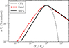 |
Fig. A.1. Comparison between different spectral models, normalised to 1 at their maxima. The low and high energy index used is α = −2/3 and β = −2.59 for all models. |
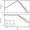 |
Fig. A.2. Qualitative behaviour of the rest frame peak energy and light curve used in our model with respect to peak time. |
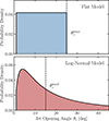 |
Fig. A.3. Example distributions for the two non-universal population models in our analysis. |
Appendix B: Impact of the constant energy assumption on non-universal jets
In our main analysis of non-universal jet geometries (Sect. 3.3), we treat the isotropic equivalent luminosity L and the jet opening angle θc as independently sampled parameters. This implies an underlying population where wider jets possess intrinsically higher true total energies. To verify that our constraints are robust against this assumption, we tested an alternative ‘constant energy’ scenario where the total energy reservoir of the central engine is conserved. In this configuration, the apparent isotropic luminosity of each simulated burst is scaled for wider jets by a factor of (1 − cos θc). Therefore the extraction of luminosity in the MCMC is conditional on the extraction of θc and this formally translates in assuming a probability distribution of the jet luminosity in the form P(L|k, L*(θc)), where L*(θc)∝1 − cos θc.
To determine if this coupling alters our constraints, we re-ran our MCMC framework for one of the models in higher tension with observations, the low-rate K265 model with high kicks (σ = 265 km/s) and αCE = 0.5, to study how this variation would affect the tension. We performed this test for both the Flat and Log-Normal non-universal jet distributions. We also performed a test on our Fiducial population and we obtained similar results.
Figure B.1 shows the joint posterior distributions for jet fraction, angle and energetics, comparing our standard baseline analysis against our analysis introducing the ‘constant energy’ assumption. We keep the nomenclature L* for the luminosity parameter, noting that by adding the shift the physical meaning is not the same.
Apart from a shift in the posterior of L*, we find that introducing the ‘constant energy’ assumption modifies the inferred median parameters by less than 15% compared to the baseline, with the remaining parameters (k, μE, σE) matching even more closely. Most importantly, the constraints on the jet fraction fj and the characteristic jet aperture remain effectively unchanged.
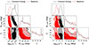 |
Fig. B.1. Posterior distributions for the K265 (αCE = 0.5) population, comparing our baseline model against the constant energy assumption where luminosity scales with 1 − cos(θc). The 1 and 2σ contours are shown. Panel (a): Flat model comparison. Panel (b): Log-normal model comparison. |
Appendix C: Fermi-GBM data
We provide the distributions of the Fermi-GBM data used in this work in Fig. C.1. As discussed in Sect. 2.4 we have very similar cuts to previous works (Salafia et al. 2023; Ronchini et al. 2022). The figure displays the complementary cumulative distribution functions for the four main observables which are peak energy, T90, fluence, and peak flux. The vertical dashed lines indicate the specific cuts applied to define our sGRB sample (Fplim ≥ 4 ph cm−2 s−1, T90 < 2 s, and Ep ∈ [50 keV, 10 MeV]). We additionally plot a dotted power law line with index −3/2 which is the behaviour expected form uniformly distributed GRBs (von Kienlin et al. 2020). This power law is used to define the peak flux cut to minimise selection effects.
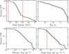 |
Fig. C.1. Inverse cumulative distributions of the observables retrieved from the Fermi-GBM catalogue. The additional quality cuts are shown with vertical red dashed lines. The dotted line shows a power law with index −3/2. |
Appendix D: Description of population synthesis models
In this work we analysed the binary population synthesis models generated by Iorio et al. (2023) using the SEVN code. These models explore the large parameter space of binary evolution uncertainties. While the original work provides a comprehensive technical description, we present here a simplified summary of the model variations most relevant to the formation of BNS mergers and their subsequent sGRB production. Table D.1 lists the model acronyms used throughout this paper and summarises the major physical assumptions and differences among the populations.
Primary physical assumption varied for each BNS population synthesis models from Iorio et al. (2023).
Appendix E: MCMC convergence and posterior predictive checks
To ensure the MCMC simulations reached a converged posterior distribution, we monitored the integrated autocorrelation time, τ, as defined in Foreman-Mackey et al. (2013). We required the total chain length to be at least 50 times greater than τ, a criterion typically satisfied within 30,000 to 40,000 iterations, indicating well-sampled posteriors. With convergence established, we performed a posterior predictive check to assess the model’s goodness-of-fit. We generated synthetic sGRB catalogues by randomly sampling parameter sets from the converged chains and comparing the resulting Empirical Cumulative Distribution Functions (ECDFs) for the four key observables against the Fermi-GBM data. We show in Fig. E.1 the simulated median and 90% credible intervals having very good agreement with the observed distributions. The test is done on our Fiducial population. This confirms that the model successfully reproduces the fundamental features of the sGRB population. The resulting posterior probability distributions for the universal structured jet and the universal top-hat models are shown in Fig. E.2 and Fig. E.3, with relative medians summarised in Table E.1.
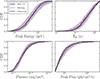 |
Fig. E.1. Cumulative distributions of the observables for real Fermi-GBM sGRBs (solid line) and simulated sGRBs associated with our fiducial BNS population. |
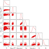 |
Fig. E.2. Posterior of the universal structured model for the fiducial population. The 1 and 2σ contours are shown. |
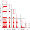 |
Fig. E.3. Posterior of the universal top-hat model for the fiducial population. The 1 and 2σ contours are shown. |
Fiducial BNS population’s median posterior values and 90% credible intervals for the sGRB emission model parameters.
It is important to note that the resulting median characteristic energy posterior has a median at E* ∼ 1048 − 1049 erg. This value may appear low compared to the canonical beaming-corrected kinetic energies of sGRBs, which are often inferred to be in excess of 1050 erg (e.g. Berger 2014). This apparent discrepancy arises directly from our model’s parameter definitions. Our E* represents the characteristic value of the radiated energy, distributed as a cut-off power-law, not the total beaming-corrected kinetic energy of the outflow. Taking into account this definition, our model produces a population of synthetic bursts whose observable fluences and fluxes are consistent with the distributions seen by Fermi-GBM.
Appendix F: Impact of physical priors on the inferred jet fraction
In our primary analysis, we allowed the jet fraction parameter fj to explore values well in excess of unity (setting the prior upper bound fmax = 10). While physically impossible, treating fj as an unbounded effective parameter is essential for quantifying the tension between BNS population models and sGRB observations.
In order to see the effect of imposing a strict physical prior (fj ≤ 1), we repeated the analysis with this constraint and we found that for models with low intrinsic merger rates (RBNS(0) ≲ 50 Gpc−3 yr−1), the posterior fj saturates against the upper boundary of 1. In contrast, models with higher intrinsic rates find their optimal fj well within the physical boundary. Figure F.1 illustrates this effect for the universal structured jet. With an unbounded prior, the median fj continuously rises as the BNS rate decreases. This allowed us to distinguish between a model that requires fj ≈ 1 (corresponding to a physical scenario where all BNS mergers produce a jet) and one requiring fj ≫ 1 (which represents a fundamental breakdown of the sole BNS-progenitor hypothesis).
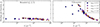 |
Fig. F.1. Comparison of the inferred median jet fraction fj as a function of total BNS rate Λ. The left panel shows bounded models, the right unbounded models. We zoom in on the region fj ∈ [0, 5] for clarity. Both cases assume a universal structured jet. |
Appendix G: Example narrowest geometry
We give a visual example on how to recover the narrowest geometry for a universal top-hat model in Fig. G.1. Given that for all models the product between jet fraction fj and beaming factor fb is monotone as a function of the structure parameter (θc, θcmax and θcmed), we can find the minimum value of these parameters to obtain a physical jet fraction.
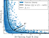 |
Fig. G.1. Narrowest geometry for the fiducial population using a universal top-hat jet. A solid line overlays the joint posterior P(θc, fj) to show the median fj as a function of θc. The intersection fj = 1 defines the minimum characteristic opening angle, θ*. |
Appendix H: Summary of model viability criteria
In this appendix we detail the criteria used to construct the summary of results presented in Table H.1. The 64 BNS population models, characterised by different binary evolution prescriptions and CE efficiencies (αCE), are evaluated based on two primary constraints. One is physical viability. A model is marked as physical (✓) if the median of its inferred jet fraction posterior distribution lies within the physical regime (median fj ≤ 1), which is equivalent to P(fj ≤ 1)≥0.5. If the median fj > 1, the model is marked as non-physical (×). For models with non-universal structure we fixed the median θc at the median value of Rouco Escorial et al. (2023, ∼6°). The other is geometric consistency. For models where the jet structure parameters are free (universal top-hat, non-universal flat, and non-universal log-normal), we assessed if the geometry required to maintain a physical fj is consistent with afterglow observations. We used the 90% credible interval upper limit from Rouco Escorial et al. (2023) of 15.4°. We classified the models using the following criteria:
-
For the universal top-hat and flat models, the index a is applied if the minimum characteristic opening angle θ* required to satisfy median fj ≤ 1 exceeds 15.4°.
-
For the log-normal model, the index b is applied if more than 10% of the inferred jet population is required to have an opening angle θc > 15° to satisfy the rate requirement.
The combination of these marks allows for a rapid identification of viable BNS populations which are those that provide enough progenitors to match the sGRB rate while maintaining jet geometries consistent with observed afterglows.
Physical viability and geometric consistency of BNS population models.
Appendix I: Redshift distribution of the average time delay
In Fig. I.1 (for physical models) and Fig. I.2 (for the remaining models), we show the redshift evolution of the average delay time, ⟨τd⟩, for each of our 64 models. Across all models, we observe that the delay times decrease by approximately two orders of magnitude as redshift increases. While the physical models exhibit the best agreement with the population averages derived by Pracchia & Salafia (2026), it is crucial to note that the average delay time is sensitive to the distribution tail. Specifically, ⟨τd⟩ can be skewed by the large delay times found at low redshifts (z < 1). Since this redshift range corresponds to the volume where sGRBs are most likely to be detected, the observed population is inherently biased towards these longer delay times, this underscores the importance of accounting for selection effects when constructing sGRB catalogues from fixed population synthesis models. A similar conclusion is reached by Pracchia & Salafia (2026), who note that selection effects, specifically when applying a peak flux cut that is too low, can bias the sample towards larger delay times.
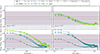 |
Fig. I.1. Average delay time ⟨τd⟩ evolution with redshift for physical population (median fj ≤ 1) assuming the universal structured jet compared to the median and 90% credible intervals inferred in Pracchia & Salafia (2026). Plots with erratic spikes have a very small number of mergers. See Table D.1 for a description of each model variation (top right of each plot). See Fig. I.2 for non physical populations. For consistency with Fig. I.2 we keep the panel for αCE = 0.5 even though no physical models exist for that value in the universal structured jet case. |
All Tables
Primary physical assumption varied for each BNS population synthesis models from Iorio et al. (2023).
Fiducial BNS population’s median posterior values and 90% credible intervals for the sGRB emission model parameters.
All Figures
|
Fig. 1. One-dimensional marginalised posterior distributions of the jet fraction fj for each considered BNS population model, assuming a universal jet structure calibrated to GRB170817A. Black lines mark medians; labels also provide the 90% C.I. values. Axes show models (x-axis) and αCE (y-axis). The colours indicate the local merger rate. |
| In the text | |
|
Fig. 2. Jet fraction statistics for the universal structured jet model assuming the GW170817/GRB170817A structure. Top row: Median jet fraction fj versus the predicted local BNS merger rate density RBNS(0) (left) and total integrated rate Λ (right). Bottom row: Quantile of the posterior distribution of fj at fj = 1 as a function of local BNS rate density (left) and total integrated rate Λ (right). Symbols are coloured according to the αCE parameter, and each symbol denotes a different population. The shaded vertical region indicates the 90% credible interval for the BNS merger rate from GWTC-4 (The LIGO Scientific Collaboration 2025). The cited fractions from the works of Ronchini et al. (2022) and Loffredo et al. (2025) are given as R22 and L25 for comparison. |
| In the text | |
|
Fig. 3. Same as Fig. 1 but with the one-dimensional marginalised distributions of ϵ = fj(1 − cos(θc)) for all the BNS populations, considering the universal top-hat jet model. For clarity log(ϵ) is shown. |
| In the text | |
|
Fig. 4. Same as Fig. 1 but assuming a universal top-hat jet with three different opening angles, θc = 5°, 10°, and 20°. These posteriors were obtained from the conditioned distribution P(fj ∣ θc) (see Fig. 3). The model LK with αCE = 0.5 does not have any samples below fj ≤ 10 for θc = 5°. |
| In the text | |
|
Fig. 5. Same as the bottom row of Fig. 2 but assuming a universal top-hat with three different aperture angles. |
| In the text | |
|
Fig. 6. Two-dimensional marginal posterior distribution P(fj, θc, max) for the non-universal flat model (left) and P(fj,θc,med) for the non-universal log-normal model (right) using our fiducial BNS population. The remaining parameters remain consistent with the results of a universal top-hat (see Fig. E.3). |
| In the text | |
|
Fig. 7. Minimum characteristic jet opening angle, θ*, required to keep the median jet fraction physical (median fj ≤ 1) as a function of the local BNS merger rate RBNS(0) for the universal top-hat (top left), non-universal flat (top right), and non-universal log-normal (bottom left). Each symbol denotes a different population. The horizontal dashed line and shaded region indicate the median and 90% credible interval of the aperture angle distribution derived from Rouco Escorial et al. (2023). Bottom right panel: Fraction of the population with wide jets (θc > 15°) for the log-normal model. The vertical grey band represents the GWTC-4 90% C.I. for the BNS merger rate. The plots do not display all 64 analysed populations, as some require θ* larger than the prior upper limit of 25°. See Table H.1 for a comprehensive list of all the populations. |
| In the text | |
|
Fig. 8. Left: Inferred intrinsic local sGRB rate RsGRB for all the BNS population models that allow physical jet fractions (with median fj ≤ 1), under the assumption of a universal structured jet. Right: Comparison of the inferred fj posterior distributions for the fiducial BNS population across the four analysed jet structures: universal structured, universal top-hat, non-universal flat, and non-universal log-normal. |
| In the text | |
|
Fig. 9. Average delay time ⟨τd⟩ for each of the 64 BNS population models compared to the median and 90% credible intervals inferred in Pracchia & Salafia (2026). The blue and red lines and ranges correspond to two models by Pracchia & Salafia (2026): a quasi-universal structured jet model and an empirical luminosity function model, respectively. To highlight the relationship between delay times and model viability, we mark with circles the populations that yield a physical jet fraction (with median fj ≤ 1) under the universal structured jet assumption and use crosses for those that are considered non-physical. |
| In the text | |
|
Fig. A.1. Comparison between different spectral models, normalised to 1 at their maxima. The low and high energy index used is α = −2/3 and β = −2.59 for all models. |
| In the text | |
|
Fig. A.2. Qualitative behaviour of the rest frame peak energy and light curve used in our model with respect to peak time. |
| In the text | |
|
Fig. A.3. Example distributions for the two non-universal population models in our analysis. |
| In the text | |
|
Fig. B.1. Posterior distributions for the K265 (αCE = 0.5) population, comparing our baseline model against the constant energy assumption where luminosity scales with 1 − cos(θc). The 1 and 2σ contours are shown. Panel (a): Flat model comparison. Panel (b): Log-normal model comparison. |
| In the text | |
|
Fig. C.1. Inverse cumulative distributions of the observables retrieved from the Fermi-GBM catalogue. The additional quality cuts are shown with vertical red dashed lines. The dotted line shows a power law with index −3/2. |
| In the text | |
|
Fig. E.1. Cumulative distributions of the observables for real Fermi-GBM sGRBs (solid line) and simulated sGRBs associated with our fiducial BNS population. |
| In the text | |
|
Fig. E.2. Posterior of the universal structured model for the fiducial population. The 1 and 2σ contours are shown. |
| In the text | |
|
Fig. E.3. Posterior of the universal top-hat model for the fiducial population. The 1 and 2σ contours are shown. |
| In the text | |
|
Fig. F.1. Comparison of the inferred median jet fraction fj as a function of total BNS rate Λ. The left panel shows bounded models, the right unbounded models. We zoom in on the region fj ∈ [0, 5] for clarity. Both cases assume a universal structured jet. |
| In the text | |
|
Fig. G.1. Narrowest geometry for the fiducial population using a universal top-hat jet. A solid line overlays the joint posterior P(θc, fj) to show the median fj as a function of θc. The intersection fj = 1 defines the minimum characteristic opening angle, θ*. |
| In the text | |
|
Fig. I.1. Average delay time ⟨τd⟩ evolution with redshift for physical population (median fj ≤ 1) assuming the universal structured jet compared to the median and 90% credible intervals inferred in Pracchia & Salafia (2026). Plots with erratic spikes have a very small number of mergers. See Table D.1 for a description of each model variation (top right of each plot). See Fig. I.2 for non physical populations. For consistency with Fig. I.2 we keep the panel for αCE = 0.5 even though no physical models exist for that value in the universal structured jet case. |
| In the text | |
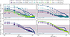 |
Fig. I.2. Same as Fig. I.1 but for non physical populations (median fj > 1). |
| In the text | |
Current usage metrics show cumulative count of Article Views (full-text article views including HTML views, PDF and ePub downloads, according to the available data) and Abstracts Views on Vision4Press platform.
Data correspond to usage on the plateform after 2015. The current usage metrics is available 48-96 hours after online publication and is updated daily on week days.
Initial download of the metrics may take a while.