


| Issue |
A&A
Volume 710, June 2026
|
|
|---|---|---|
| Article Number | A343 | |
| Number of page(s) | 14 | |
| Section | Planets, planetary systems, and small bodies | |
| DOI | https://doi.org/10.1051/0004-6361/202659264 | |
| Published online | 26 June 2026 | |
New 12C/13C and 14N/15N isotopic ratios measurements in HCN in the Jupiter stratosphere revealed by ALMA
1
Laboratoire d’Astrophysique de Bordeaux, Univ. Bordeaux, CNRS, B18N, allée Geoffroy Saint-Hilaire,
33615
Pessac,
France
2
LIRA, Observatoire de Paris, Université PSL, CNRS, Sorbonne Université, Université Paris Cité,
5 place Jules Janssen,
92195
Meudon,
France
3
Max-Planck-Institute for Solar System Research,
Göttingen,
Germany
★ Corresponding author: This email address is being protected from spambots. You need JavaScript enabled to view it.
Received:
2
February
2026
Accepted:
12
May
2026
Abstract
Context. The collision of comet Shoemaker-Levy 9 (SL9) with Jupiter in 1994 changed the chemical composition of the Jovian stratosphere for decades. New molecules were detected minutes after the impacts (HCN, CO, H2O, CS, etc.) and some are still present today. They were deposited in the stratosphere at pressures lower than 0.1 mbar and were most probably formed by shock-induced chemistry recombining Jovian and cometary material. However, the question of the origin of these molecules is still not completely understood. One way to address this open question is to determine the isotopic composition of the new molecules. Isotopic ratios have long been measured in the Solar System. They present a variety of values depending on the object or the molecule and therefore trace different reservoirs of material. Derivations of carbon and nitrogen isotopic ratios in HCN four years after SL9 showed atypical depletions in the heavier isotopes that had never been observed before in the Solar System. These results suggested an unusual cometary composition or an unknown fractionation mechanism in the hot and shocked air parcels.
Aims. We aim to measure carbon and nitrogen isotopic ratios in HCN to shed light on the puzzling results of 1998.
Methods. With Atacama Large Millimeter/submillimeter Array data from 2017 and radiative-transfer calculations, we derived the abundance of two HCN isotopologues, H13CN and HC15N, at pressures probed from 0.03 to 1.8 mbar.
Results. We find 12C/13C = 73 ± 5 and 14N/15N = 245 ± 29, respectively (0.76–0.87) and (0.80–1.00) times the terrestrial references, and (0.69–0.87) and (0.42–0.70) times the solar-Jovian bulk values. In contrast to the strong depletions reported in 1998, our values are instead compatible with an enrichment in the heavier isotopes relative to the Jovian bulk.
Conclusions. We interpret these enrichments as the direct signature of the cometary contribution in HCN and/or as 23 years of chemical evolution in the Jovian atmosphere.
Key words: planets and satellites: atmospheres / planets and satellites: individual: Jupiter
© The Authors 2026
 Open Access article, published by EDP Sciences, under the terms of the Creative Commons Attribution License (https://creativecommons.org/licenses/by/4.0), which permits unrestricted use, distribution, and reproduction in any medium, provided the original work is properly cited.
This article is published in open access under the Subscribe to Open model. This email address is being protected from spambots. You need JavaScript enabled to view it. to support open access publication.
1 Introduction
Jupiter and the other giant planets are constantly subject to external modifications that enrich their atmosphere with new material (e.g. Lellouch et al. 1995; Hesman et al. 2007; Hartogh et al. 2011; Cavalié et al. 2010, 2014; Moses & Poppe 2017). A major example consisted of the 21 fragments of the comet Shoemaker-Levy 9 (SL9), which impacted the Jupiter atmosphere in July 1994 at 44°S during a week (Noll et al. 1996). Molecules that were previously undetected in the stratosphere of Jupiter (H2O, CS, HCN, OCS, and many more) were observed minutes, months (see the review of Lellouch 1996), and, for the most long-lived, years after the impacts (Lellouch et al. 2002, 2006; Moreno et al. 2003; Iino et al. 2016; Cavalié et al. 2013, 2023; Benmahi et al. 2020; Rodríguez-Ovalle et al. 2025). Other molecules that were already present before SL9, such as CO (Bézard et al. 2002), saw their stratospheric abundance enhanced after the impacts (Lellouch et al. 1997). These molecules are the direct tracers of the dynamical and chemical processes triggered by the impacts (Zahnle 1996; Lellouch 1996). Therefore, their study during and after the impacts can make it possible to reconstruct their formation and/or deposition history and their further temporal and spatial evolution in the Jovian atmosphere.
The question of the origin of these molecules, i.e. from which reservoir of material (Jovian or cometary) and in which conditions (explosion, fireball, splashback, etc.) they were formed, is still open as it involves many parameters. Firstly, the elementary composition of the comet was not known before the impacts (Crovisier 1996) and some hints can only be found during or after the impacts in the new material formed/deposited in the Jovian atmosphere (Lellouch 1996). However, the cometary material completely mixed with the Jovian air in the impact fireball, making it difficult to separate the cometary from the Jovian contribution in the newly formed species (Lellouch et al. 1995; Crovisier 1996). In addition, the different phases of impact (fragment entry, final explosion, rising fireball, plumes fallback) led to different physical processes (Zahnle 1996) and thus altered the atmosphere differently depending on the altitude and horizontal extent at which they occurred. For example, CS, CO, and HCN were probably formed by shock-induced chemistry (Zahnle 1996), recombining cometary and Jovian material in the extreme conditions of the fireball and plumes splashback in which temperatures reached several thousands of kelvins (Chapman 1996; Bjoraker et al. 1996; Nicholson 1996). They were all deposited during the plumes’ re-entry into the stratosphere at pressures of 0.05–0.2 mbar (Lellouch et al. 1997). In this case, it becomes difficult to decipher the relative contributions of cometary and Jovian materials to the final products (Lellouch 1996). On the other hand, the detection of NH3 and H2S (normally only present in Jupiter’s troposphere) in the lower stratosphere suggested that convection driven by the heat released at a few bars by the fragment explosion overshoot to the lower stratosphere and transported here Jovian air and cloud materials (Yelle & McGrath 1996; Griffith et al. 1997). In this case, the lower stratospheric NH3 and H2S probably have a purely Jovian origin.
In addition, after the formation and deposition of the species at a given altitude, their initial distribution was modified as a function of time by dynamics and chemistry. The photolysis of the short-lived species (e.g. NH3) led with time to the enrichment in other species (e.g. HCN; Moreno et al. 2003; Lellouch et al. 2006; Moses 1996), thus altering the primordial composition of the new species and making it even more difficult to assess the origin of their material. Also, at first confined to the impact sites, the species spread out with longitude within a few months after the impacts and with latitude to cover the entire disc years later (Moreno et al. 2003; Lellouch et al. 2006; Cavalié et al. 2023).
In this context, measuring the isotopic composition of the new stratospheric species can still provide insights into their formation processes and their dominant sources of elements (Jovian or cometary), but the isotopic ratios can also diagnose the temporal evolution of the exogenic molecules from interactions in the Jovian atmosphere. Isotopic ratios are often used to trace the origin of a material because they reflect the physical and chemical conditions in which their bearing molecule was formed (Nomura et al. 2023). They are usually compared to solar values (Marty et al. 2011; Lyons et al. 2018) or to the Earth references (IAEA 1995; Coplen et al. 1992) to reveal any fractionation processes as a function of the type of object, the distance to the Sun, or the molecule (Nomura et al. 2023). Only the carbon, nitrogen, and sulphur isotopic ratios were estimated four years after SL9 impacts in exogenic HCN and CS by Matthews et al. (2002). They derived an abnormal depletion in all three heavier isotopes (13C, 15N, 34S), with 12C/13C, 14N/15N, and 32S/34S ratios nominally higher by factors of three, ten, and three, respectively, than the Earth references of 89, 272, and 23.
Isotopic ratios have been estimated in a wide range of Solar System objects and in several of their molecules over the past 50 years. For example, there is a general trend that the 12C/13C ratio is quasi-constant throughout the Solar System at a value close to solar and terrestrial, independently of the object (meteorites, comets, giant, and terrestrial planets) or the molecule (Nomura et al. 2023; Woods & Willacy 2009; Woods 2009). This absence of notable isotopic fractionation seems to indicate that the Solar System objects accreted carbon from a common reservoir, or that all carbon reservoirs present the same isotopic composition (Fletcher et al. 2009; Nomura et al. 2023). A departure from this common trend, as reported by Matthews et al. (2002) in the carbon present in the SL9-produced HCN, is thus very intriguing. On the other hand, the nitrogen isotopic composition presents a broader range of values in the Solar System and is highly dependent on the type of the object. In the giant planet atmospheres, the 14N/15N ratio is close to solar but is super-terrestrial by a factor of 1.6 (Owen et al. 2001; Fouchet et al. 2000; Fletcher et al. 2014). Comets are the most 15N-enriched objects of the Solar System. Their 14N/15N nominal values are at least a factor of two lower than the terrestrial reference and a factor of three lower than the solar and Jovian values (Hily-Blant et al. 2017). The dispersion of values in the nitrogen isotopic ratio among Solar System objects is thus helpful to decipher the origin of the objects, as opposed to the carbon ratio. However, as for carbon, the strong depletion in 15N in HCN after SL9 completely departs from any Solar System measurements, even from the Jovian bulk, which is the least enriched. Unfortunately, no complementary observations of the isotopic ratios in Jupiter’s exogenic molecules have been performed these past 30 years. The results of Matthews et al. (2002) thus remain puzzling and no definitive answer has been found regarding the origin of the elements composing HCN.
In this work, we used 2017 Atacama Large Millimeter/submillimeter Array (ALMA) observations of HCN and two of its isotopologues, H13CN and HC15N, to estimate the carbon and nitrogen isotopic ratios in HCN in the Jupiter stratosphere 23 years after SL9 impacts, and to try to understand the intriguing results of Matthews et al. (2002) in 1998. We detail the dataset in Section 2 and the radiative-transfer model used to simulate the observations in Section 3. We then present the results in Section 4 and discuss and compare them to other measurements in Section 5. We give our conclusions in Section 6.
2 Observations
We used the ALMA Cycle 4 dataset already presented in Cavalié et al. (2021, 2023) from which they derived, respectively, stratospheric wind measurements and vertical abundance profiles from the CO (J=3–2) line at 345.7960 GHz and the HCN (J=4–3) line at 354.5055 GHz. General information on the dataset is presented here, but more details on the observation setup and data reduction can be found in Cavalié et al. (2021, 2023).
The Jupiter observations were recorded on March 22, 2017 as part of the 2016.1.01235.S project. The ALMA configuration at the time of the observations consisted of 42 antennas with a diameter of 12 m and baselines extending from 15.1 to 160.7 m. The resulting beam size is 1.0–1.2″ (east-west and north-south) with a position angle of 87.3°. The complete dataset consists of four different spectral cubes of Jupiter, taken in four spectral bands, from which we extracted two smaller cubes at 345.3398 and 344.2003 GHz encompassing, respectively, the H13CN and HC15N (J=4–3) lines. These are the only isotopic lines present in the dataset. The continuum level was subtracted from these cubes. The spectral resolution is Δν = 0.488 MHz, resulting in a spectral resolving power of about 7 × 10⁵ at 344–345 GHz.
Jupiter’s angular diameter was 43.8″ at the equator, and its rotation axis was tilted by 23.7°1. The sub-observer latitude was −3.5° and the sub-observer longitude was 65.4°W2 at the beginning of the observation. During the 24 min on-source integration time, the planet rotated by 15°; we thus observed the planetary western limb in a longitude range spanning 155–170°W and 335–350°W at the eastern limb.
The small beam size compared to the planet’s disk resulted in a latitudinal resolution of 2–3° per beam at the low latitudes and up to 8° per beam at the higher latitudes. From the knowledge of Jupiter’s geometry and using the continuum map of Jupiter, we found a pointing offset of ΔRA=0.053″ and ΔDec=−0.039″ and re-centred the planetary disc accordingly. For both spectral cubes (H13CN and HC15N), we oversampled the beam by a factor of four and extracted 540 spectra at the planetary limb, which is defined by the projected planetary ellipse at the 1 bar level. We only extracted spectra at the limb where we have the highest line sensitivity.
The same procedure was performed by Cavalié et al. (2023) to extract HCN spectra at the limb. Because the spatial resolution is slightly better at the HCN (J=4–3) transition, they extracted a total of 557 limb spectra. The total 24 min observation time was sufficient to detect the HCN line in each of these individual limb spectra and reach signal-to-noise ratios (SNR) of the order of 25 per beam. An example of an HCN individual spectrum is presented in Fig. 1. However, because H13CN and HC15N are significantly less abundant than H12C14N, the resulting lines are too faint to be detected in an individual limb-extracted spectrum. Therefore, to increase the SNR, we needed to co-add spectra, and we adopted the following procedure: (1) for each spectrum and on both limbs, we subtracted the Doppler shift caused by the beam-convolved planet rotation to re-centre all the lines at the line rest frequency; then (2) we averaged the spectra on the selected latitudinal range that gives the best SNR; and (3) we subtracted any continuum baseline left with the averaging step. The best latitudinal range was found to be 50°S-50°N (i.e. 303 selected spectra) and corresponds to the highest and rather constant HCN column density with latitude (Cavalié et al. 2023). The final spectra obtained with this method are illustrated in Figs. 1 (right), 2, and 3 for HCN, H13CN, and HC15N, respectively. We detected the H13CN and HC15N lines with an SNR at a line peak of 24 and five, respectively, and with noise levels at 1σ of 2.1 and 2.6 mJy/beam.
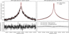 |
Fig. 1 HCN limb spectra. (left) HCN limb spectrum extracted at a single position on the eastern equatorial limb at 3°N. (right) HCN spectrum averaged over the two limbs and on the latitudinal range 50°S-50°N. The observed spectra are presented in black and the modelled spectra in red. The differences between the observed and the modelled spectra are shown below with the residuals. The 0 Jy/beam level is depicted by the thin solid black line. The dashed-dotted lines represent the 1σ noise level in the single spectrum on the left panel, and the dashed lines the 1σ noise level from the right panel’s averaged spectrum. For the single pointing spectra, the continuum level was subtracted and the lines were centred at the rest frequency. The averaged spectra follow the same averaging method described in Section 2. Observations come from the dataset presented in Cavalié et al. (2023). Modelled spectra were computed with the procedure detailed in Section 3. |
3 Modelling
We used the radiative-transfer model detailed in Cavalié et al. (2019) (and references therein) to simulate the HCN, H13CN, and HC15N lines in the same atmospheric, geometric, and instrumental conditions of the observations. The most important code inputs are summarised in Section 3.1. As the isotopologue lines are optically thin (the opacities at the line centre are 0.015 and 0.004, respectively), the line amplitude is sensitive to the atmospheric temperature and to the abundance of the species. We detail the 3D fields employed in the modelling in Sections 3.2 to 3.4.
3.1 Radiative-transfer model
The radiative transfer model from Cavalié et al. (2019) is a line-by-line model accounting for Jupiter’s 3D ellipsoidal geometry in the same conditions as the observations (see Section 2). The background composition of H2, He, CH4, NH3, and PH3 used for the continuum is the same as in Cavalié et al. (2023).
The pressure broadening coefficient, γ, and the exponent for the temperature dependency, denoted n, were not measured for the H13CN and HC15N (J=4–3) transitions. Rohart et al. (1987) only gave values for the J=1–0 transition of HC15N: γ = 0.1308 cm−1.atm−1 and n = 0.752. Here for consistency, in the nominal model, we adopted the pressure-broadening parameters of the H12C14N (J=4–3) transition from Rohart et al. (1987) (and used by Cavalié et al. 2023) for both heavier isotopologues, i.e. γ = 0.1447 cm−1.atm−1 and n = 0.756. In addition, we rescaled the HC15N (J=1–0) parameters using the H12C14N (J=1–0) and (J=4–3) values to estimate the parameters at the HC15N (J=4–3) transition: γ = 0.1305 cm−1.atm−1 and n = 0.770. The difference implied on the derived HC15N abundance by choosing either these rescaled values or the nominal ones is accounted for in the uncertainties. In the absence of information on the H13CN parameters, the same approach as for HC15N was performed for H13CN.
We computed spatially and spectrally convolved spectra of H13CN and HC15N at each of the 303 selected positions extracted from the limb, contained between 50°S and 50°N. The modelled continuum level was removed by subtracting a linear slope under the lines. Modelled spectra were then corrected for the beam-convolved planet rotation and co-added following the same method as for the observations, on the same latitudinal range.
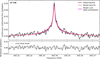 |
Fig. 2 (Top) Observed and modelled spectra of the H13CN line at 345.3398 GHz. The observed spectrum is depicted by the black line and corresponds to a latitudinal average on the 50°S-50°N range from both limbs. The modelled spectrum that best fits the observations is represented by the solid red line. The pink area shows the ±2σ uncertainties on the modelled line. (Bottom) Residuals corresponding to the difference between the observed spectrum and the model’s best fit. The horizontal dotted black lines represent the ±1σ noise level in the averaged spectrum. |
3.2 Thermal field
The latitude-pressure thermal field used in this paper is presented in more detail in Cavalié et al. (2023). The data were retrieved from IRTF/TEXES observations (Cosentino et al. 2017; Sinclair et al. 2023), which were taken near-simultaneously to the ALMA dataset. The thermal vertical profiles inverted from these data span 1 μbar to 1 bar with a 2 K uncertainty (Cosentino et al. 2017). The final thermal field consists of two 2D latitude-pressure fields (one at each planetary limb) re-gridded on a 1° latitude grid (see Extended Data Fig. 1 in Cavalié et al. 2023).
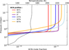 |
Fig. 4 Selection of H12C14N vertical profiles used in our radiative-transfer modelling at different latitudes and all (arbitrarily) taken from the eastern limb. They illustrate the limited variety of profiles retrieved at all low-to-mid latitudes on both limbs, as shown in Cavalié et al. (2023). The filled areas show the 1σ envelope resulting from the 1σ uncertainties on the retrieved profile parameters. A typical temperature profile extracted at the equator is also displayed on the top x-axis as an example (dashed black line). The full 3D temperature field can be found in Cavalié et al. (2023). |
3.3 H12C14N abundance field
We used the H12C14N latitude-pressure abundance field determined by Cavalié et al. (2023) from the same ALMA dataset of March 22, 2017, at both limbs. Their retrievals were performed at 557 positions, which were extracted at the planetary limb from a beam oversampling of a factor of four. The HCN observations benefit from a high spectral resolving power of 3 × 10⁶ that enables us to resolve the true line shape, which in turn allows us to retrieve the vertical distribution of HCN. Each of their 557 HCN spectra were fitted with an inversion algorithm coupled to the radiative-transfer model presented above, in which the HCN vertical profile was parametrised with three parameters, a1, a2, and a3, and the following relationship:
![Mathematical equation: $\[y_{\mathrm{HCN}}(z)=a_1 \times\left(1+\tanh \left(\frac{z-a_2}{2 a_3}\right)\right),\]$](/articles/aa/full_html/2026/06/aa59264-26/aa59264-26-eq1.png)
where yHCN is the HCN abundance or volume mixing ratio (VMR), z is the altitude in km above the 1-bar level, a1 is half the asymptotical high-altitude HCN VMR, a2 is a cut-off level between the upper and lower stratosphere, and a3 indicates the steepness of the slope at the cut-off level, with a stronger slope for larger a3 values. Examples of these retrieved HCN vertical profiles are presented in Fig. 4. The uncertainties on the retrieved vertical profiles come from the combination of several sources: (i) flux-calibration uncertainties, which are reported at a level of 5%; (ii) retrieval uncertainties on the a1, a2, and a3 parameters resulting from the spectral noise and which translate to an approximately 5% uncertainty on the retrieved abundances. It should be noted that, even though the HCN line has an opacity of 1.6 at the line centre in the low-to-mid latitudes, any line saturation is accounted for when retrieving the uncertainties on the vertical profile parameters; (iii) uncertainties resulting from the 2 K uncertainty on the temperature field, which translate into a 1% uncertainty on the abundances; (iv) the uncertainties resulting from the continuum subtraction in the uv-plane during the data analysis. This was reported by Cavalié et al. (2023) to be the largest source of uncertainties on the retrieved abundances, causing a 30% uncertainty on the abundances. Considering all four contributions, there is an overall 40% uncertainty on the HCN vertical profiles.
With the individual HCN vertical profiles of Cavalié et al. (2023), the final HCN abundance field used in our radiative-transfer calculations consists on two 2D latitude-pressure fields (one at each limb), re-gridded with a 1° latitude step, as for the thermal field. This was done by co-adding vertical profiles located within each 1° latitude step. Because the latitudinal resolution is 2–3° in one beam in these observations, and because the beam was oversampled by a factor of four in the HCN profile retrieval process, it means that each 1° latitude step of our grid averages two retrieved profiles on average.
To ensure that the re-gridded HCN field presented above was valid, we ran radiative-transfer calculations for the HCN line at each of the 557 positions. As an example, Fig. 1 shows a model-observation comparison for the east-equatorial spectrum. After applying the spectrum-averaging method described in Section 2, we obtained the result shown in Fig. 1 right. The co-addition of individual spectra results in a significant decrease of the noise level, from 0.043 mJy/beam on a single spectrum, to 0.004 mJy/beam on the averaged one. As a consequence, the mismatches that lied within the noise on individual spectra result in differences after the averaging stage that then become more significant (see the residual on Fig. 1, right). However, those differences remain very limited. This demonstrates that the HCN abundance field can be used as a reference to derive the isotopologue abundances and consequently compute the 12C/13C and 14N/15N isotopic ratios.
3.4 H13CN and HC15N abundance field
We assume H13CN and HC15N have the same vertical and horizontal distribution as the 3D H12C14N abundance field detailed above, but rescaled by a constant factor representing the isotopic ratio. Fractionation from condensation with altitude was excluded for two reasons: (1) the HCN vapour pressure curve (see Jancso & Van Hook 1974; Fray & Schmitt 2009; Hudson & Gerakines 2023) indicates that the molecule is far from condensing under Jovian stratospheric temperature and pressure conditions (about 170 K at 0.1 mbar), with mole fractions of the order of 10−11 − 10−9; and (2) vapour pressure curves between isotopologues are typically very similar. Saturation curves from Jancso & Van Hook (1974) (and references therein) indeed indicate a difference of the order of 10% between the HCN and HC15N curves, which is still very far from the Jovian atmospheric conditions. The same is expected for H13CN, of which the vapour pressure is unknown. Other isotopic fractionation processes (photolysis and neutral or ionic chemistry) can change the isotopic distribution as a function of altitude. It is the case for the N-bearing molecules in the N2 rich atmosphere of Titan, but the fractionation occurs at very high altitudes, where isotopic ratios are sensitive to magnetospheric electrons (Nosowitz et al. 2025; Dobrijevic & Loison 2018). In the stratosphere of giant planets, these effects in the C- and N-bearing molecules, such as HCN, are poorly known and more unlikely in the 50°S-50°N latitude range adopted here, compared to auroral regions. Here, in the absence of observational or theoretical evidence, and to limit the number of parameters to adjust, we did not consider any isotopic fractionation effects as a function of altitude.
Therefore, we derived the H12C14N/H13C14N (resp. H12C14N/H12C15N) ratios by rescaling the H12C14N field until the H13C14N (resp. H12C15N) line was fitted. The isotopic ratios of carbon and nitrogen in HCN are then simply the following:
![Mathematical equation: $\[\frac{y_{\mathrm{H}^{12} \mathrm{C}^{14} \mathrm{N}}}{y_{\mathrm{H}^{13} \mathrm{C}^{14} \mathrm{N}}}=\frac{{ }^{12} \mathrm{C}}{{ }^{13} \mathrm{C}} \quad \text { and } \quad \frac{y_{\mathrm{H}^{12} \mathrm{C}^{14} \mathrm{N}}}{y_{\mathrm{H}^{12} \mathrm{C}^{15} \mathrm{N}}}=\frac{{ }^{14} \mathrm{N}}{{ }^{15} \mathrm{N}}.\]$](/articles/aa/full_html/2026/06/aa59264-26/aa59264-26-eq2.png)
4 Results
We ran radiative-transfer calculations to find the isotopic ratios that best fit the observations. The results for 12C/13C and 14N/15N are the following:
![Mathematical equation: $\[\begin{aligned}&\begin{aligned}\frac{{ }^{12} \mathrm{C}}{{ }^{13} \mathrm{C}} & =73 \pm 5 \\& =(0.76\mathrm{-}0.87) \times 89.0 \text { (Earth ref.) } \\& =(0.72\mathrm{-}0.83) \times 93.5 \text { (Sun) } \\& =(0.69\mathrm{-}0.87) \times 92.6 \text { (Jupiter)},\end{aligned}\\\\&\begin{aligned}\frac{{ }^{14} \mathrm{N}}{{ }^{15} \mathrm{N}} & =245 \pm 29 \\& =(0.80\mathrm{-}1.00) \times 272.0 \text { (Earth ref.) } \\& =(0.48\mathrm{-}0.63) \times 440.9 \text { (Sun) } \\& =(0.42\mathrm{-}0.70) \times 434.8 \text { (Jupiter)}.\end{aligned}\end{aligned}\]$](/articles/aa/full_html/2026/06/aa59264-26/aa59264-26-eq3.png)
The present isotopic ratios are compared to the reference terrestrial values of 89 for carbon and 272 for nitrogen (IAEA 1995; Coplen et al. 1992), to the solar values of 93.5 ± 0.7 and 440.9 ± 5.4 (Lyons et al. 2018; Marty et al. 2011), and to the Jovian bulk values from the Galileo entry probe of 92.6 ± 4.3 and 434.8 ± 56.7 (Niemann et al. 1998; Owen et al. 2001). In Jupiter, those ratios were measured in CH4 and NH3, respectively, as the major C- and N-bearing species in Jupiter’s troposphere. Additional references are found in Tables A.1 and A.3 for the Jovian bulk. The comparison factors encompass the uncertainties of our derived values in the Jovian exogenic HCN and the uncertainties on the object of comparison (the Earth, Sun, or Jupiter).
We took into account three types of uncertainties that we quadratically added: (1) the natural fitting uncertainty arising from the noise level in the spectrum (at ±1σ); (2) the error arising from the uncertainties on the individual HCN vertical profiles derived by Cavalié et al. (2023) (see Section 3.3); and (3) the uncertainty that arises from the choice of pressure broadening parameters γ and n (see Section 3.1). In order to avoid overestimating the second source of uncertainty when performing the average of the spectra on the 50°S-50°N latitudinal range, we divided by the square-root of the number of independent pointings in this range (=303/4).
For HC15N, the major source of uncertainty resides in the noise level (about 70% of the total error), followed by the effect of the broadening parameters and the uncertainty on the HCN profile (about 15%). In the case of H13CN, the uncertainty arising from the noise level accounts for ~10%, the rest being due to the broadening parameters and the uncertainty on the HCN profile (about 40% each). Averaging the spectra from 50°S to 50°N considerably reduces the impact of the individual HCN vertical profile uncertainties. The uncertainties on the thermal field are already accounted for in the HCN vertical profile uncertainties (Cavalié et al. 2023). The best fits to the data are shown in Figs. 2 and 3. Computations of χ2/N values around the line centre give 1.0 and 0.7, respectively, for the H13CN and HC15N lines.
The above results are representative of the 12C/13C and 14N/15N values in the carbon and nitrogen present in the HCN molecule in Jupiter at the observation date. Computations of the contribution functions, averaged on 50°S-50°N, indicate that for both isotopologues 60% of the line emission originates from the 0.03–1.80 mbar range, with a peak at 0.25 mbar. Implications of these results are presented in the next section.
5 Discussion
Stratospheric HCN is an exogenic species that was formed in extreme conditions from a Jovian air–cometary mixture (Gautier et al. 1995; Zahnle 1996) and has continuously evolved in the Jovian stratosphere ever since (e.g. Moreno et al. 2003; Lellouch et al. 2006; Cavalié et al. 2023). Therefore, the interpretation of the isotopic ratios in HCN is particular here; their values years after SL9 can give information on the Jovian–comet mixture at the origin of HCN or on the high pressure or temperature chemistry of the shock, but in principle they can also reflect the history of HCN and its isotopologues in the Jovian stratosphere. These two interpretations, i.e. origin and evolution, are discussed in this section.
In this context, we now have two data points for the 12C/13C and 14N/15N ratios in HCN, one from 1998 observations (Matthews et al. 2002), and one from 2017 data. No observations of the heavier isotopologues of HCN (or of any other exogenic species containing carbon or nitrogen) were made right after the collisions; hence, we do not have any direct constraints on the isotopic composition at that time and we can only rely on later measurements. A comparison of the 1998 and 2017 results shows a contradictory behaviour; i.e. while the Matthews et al. measurements suggest an atypically strong depletion in both 13C and 15N relative to the Jovian bulk, our new estimates instead indicate an enrichment compared to Jovian values. In what follows, we first discuss the validity of the 1998 results in Section 5.1. We explain why we eventually chose to discard them. We then give our interpretation of the 2017 results alone in Section 5.2.
5.1 Implications of the 1998 measurements
The first observations of H13CN and HC15N were taken in September 1998, four years after the SL9 impacts, by Matthews et al. (2002). They found the following ranges of values:
![Mathematical equation: $\[\begin{aligned}&\begin{aligned}\frac{{ }^{12} \mathrm{C}}{{ }^{13} \mathrm{C}} & =176\mathrm{-}409 \\& =(2.0\mathrm{-}4.6) \times 89~(\text {Earth ref.}) \\& =(1.9\mathrm{-}4.4) \times 93.5~(\text {Sun}) \\& =(1.8\mathrm{-}4.6) \times 92.6~(\text {Jupiter}),\end{aligned}\\\\&\begin{aligned}\frac{14 \mathrm{N}}{15 \mathrm{N}} & =1150\mathrm{-}4500 \\& =(4.3\mathrm{-}16.7) \times 272~(\text {Earth ref.}) \\& =(2.5\mathrm{-}10.3) \times 440.9~(\text {Sun}) \\& =(1.8\mathrm{-}11.2) \times 434.8~(\text {Jupiter}).\end{aligned}\end{aligned}\]$](/articles/aa/full_html/2026/06/aa59264-26/aa59264-26-eq4.png)
Their results are compared to the Earth reference and to the solar and Jovian bulks, in the same way as in Section 4. Figs. 5 and 6 present determinations of the carbon and nitrogen ratios in various Solar System objects (more details are found in Tables A.1–A.3 and references therein). The Jovian atmosphere is well known to present solar values both for carbon and nitrogen (see the most accurate results from the in situ measurements of the Galileo entry probe (Niemann et al. 1998; Owen et al. 2001); a Jovian source was consequently ruled out. Matthews et al. (2002) interpreted the ratios to originate from an unusual cometary composition or an unknown isotopic fractionation process during the different phases of the impacts. We discuss the two hypotheses below and also give other interpretations.
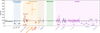 |
Fig. 5 Review of 12C/13C ratio in the various Solar System objects. Detailed information on the instrument, the observation date, and the references are reported in Tables A.1 (giant planets only) and A.2 (the other Solar System determinations) and references therein. |
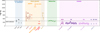 |
Fig. 6 Review of 14N/15N ratio in the various Solar System objects. Detailed information on the instrument, the observation date, and the references are reported in Table A.3 and references therein. |
5.1.1 An unknown isotopic fractionation during the impacts
Firstly, one possibility is that a fractionation mechanism in the shocks could have preferentially enriched HCN in the lighter isotopes (12C and 14N), probably through interactions with the dust, as suggested by Moreno et al. (2003). However, this hypothesis would need to be confirmed by laboratory experiments and/or plume modelling. Such work should explain why C, N, and S seem to be affected by this depletion process similarly, even if their isotopic ratios are usually very different. Until then, this possibility is still open.
5.1.2 An unusual comet composition
More than 20 years since Matthews et al. (2002), we now have access to tens of derivations in different comets and in several molecules. Among these, one can note the in situ data of the comet 67P/Churyumov–Gerasimenko in various molecules. All the measurements show Earth-like values for carbon, and the nitrogen ratio is systematically enriched in 15N (as measured in several N-bearing compounds) with respect to the terrestrial value with factors up to five, and this is, on average, with a factor of two (see Figs. 5 and 6). For the 12C/13C ratio, only Biver et al. (2016) nominally found a depletion in the comet C/2012 F6 (Lemmon) with respect to the terrestrial value, but their error bars are very large (124±64) compared to many other estimates, and they still encompass the terrestrial value. For the 14N/15N ratio, even the highest cometary values (e.g. 205 ± 70 in HCN in comet C/1995 01 (Hale–Bopp; Hily-Blant et al. 2017) are at least more enriched in 15N by a factor of five compared to those of Matthews et al. (2002). An unusual cometary source for the carbon and nitrogen content in HCN, as proposed by Matthews et al. (2002), is thus highly improbable with regard to all these comet measurements.
5.1.3 A temporal evolution of HCN between 1994 and 1998
Another potential explanation may derive from a temporal evolution of the total mass of HCN after the comet impacts of 1994, altering the isotopic composition of HCN. Continuous observations after the collisions indicated that the total mass of HCN increased by a factor up to six (Moreno et al. 2003) ten months after SL9, compared to the initial HCN mass derived by Bézard et al. (1997). The same amount was still observed in September 1998 by Moreno et al. (2003) and was consistent with the Cassini/CIRS observations at the end of 2000 (Lellouch et al. 2006 indicated an increase by a factor of ![Mathematical equation: $\[5.5_{-2.5}^{+5.0}\]$](/articles/aa/full_html/2026/06/aa59264-26/aa59264-26-eq5.png) ). As discussed extensively in Lellouch et al. (2006), the main explanation of the HCN enhancement is the conversion of Jovian NH3 (Moses 1996) which was observed in the upper stratosphere after SL9 (Griffith et al. 1997).
). As discussed extensively in Lellouch et al. (2006), the main explanation of the HCN enhancement is the conversion of Jovian NH3 (Moses 1996) which was observed in the upper stratosphere after SL9 (Griffith et al. 1997).
This additional production of HCN from NH3 should ultimately have modified the isotopic composition of the initial SL9-produced HCN. With very simple considerations, we can give an estimation of the isotopic ratios of the initial SL9-produced HCN, noted IRi. The values of Matthews et al. (2002), denoted IRf, are taken as the isotopic ratios of the total amount of HCN in 1998 (after the NH3 conversion). The additional NH3-produced HCN should present the typical ratios of the Jovian NH3 and CH4 denoted IRa, taken here as the values measured by the Galileo entry probe (see Tables A.1 and A.3). The isotopic ratios of the initial SL9-produced HCN are written as follows (for carbon or nitrogen):
![Mathematical equation: $\[\mathrm{IR}_i=\left(\frac{n}{\mathrm{IR}_f}+\frac{1-n}{\mathrm{IR}_a}\right)^{-1},\]$](/articles/aa/full_html/2026/06/aa59264-26/aa59264-26-eq6.png)
where n is the enrichment factor of HCN between the initial SL9-produced amount and the total amount of HCN several months after the impacts. The above formula is only valid for n ≥ 1, because no loss factor of HCN is considered. Values of n lie between 0.6 and six following the results of Moreno et al. (2003) and between three and 10.5 according to Lellouch et al. (2006). As a consequence, we considered n ranges between three and six.
Considering the uncertainties on IRf and IRa, IRi presents only negative (i.e. non-physical) values for n > 1.9 for carbon and for n > 1.4 for nitrogen. Positive values can exist only if n is close to one; in this case, the initial ratios become even higher than those of Matthews et al. (2002), rendering them even more incompatible with values measured in comets. In addition, such values for n are incompatible with the range resulting from Moreno et al. (2003) and Lellouch et al. (2006). In conclusion, the changes in the HCN abundance in the years after the impacts cannot explain the abnormal isotopic ratios reported by Matthews et al. (2002).
5.1.4 A possible modelling issue
Matthews et al. (2002) analysed HCN (J=4–3) and CS (J=7–6) spectra obtained at the equatorial limb and at the planet’s disc centre with the James Clerk Maxwell Telescope (JCMT). The half power beam width (HPBW) was 13″.5, and the angular diameter of Jupiter was 50″, resulting in a covered latitudinal range of 10°S-10°N. At the time of their observations, HCN had already spread out latitudinally and was present up to northern mid-latitudes with a mixing ratio of about 10−8 (Moreno et al. 2003).
Independent temperature information was unavailable for the modelling of their observations. As a consequence, Matthews et al. (2002) simultaneously derived the temperature vertical profile and the HCN and CS abundance vertical profiles directly from the HCN and CS lines using the different observation geometries (limb vs. nadir). They used simple constant vertical profiles for P0<0.2 mbar both for the temperature and the HCN abundance. Because the H12C14N line was optically thick (τ ~ 10 at the line centre), the H12C14N abundance that is derived is strongly tied to the retrieved temperature. In addition, the P0 cut-off pressure derived from the line width also shows some dependency on the temperature. Thus, several solutions can be found simultaneously for the temperature, the HCN abundance, and P0. To illustrate this point, Matthews et al. (2002) found an HCN abundance ranging from (3.0–4.5)×10−8 for a temperature of 164 ± 2 K at P0<0.2 mbar, while a reanalysis in Moreno et al. (2003) indicated (0.8–2.5)×10−8 for a temperature of 167 ± 1 K at P0<0.3 mbar for the same dataset. Our conclusion is that the abundance of H12C14N used to compute the isotopic ratios might not be well constrained, and this immediately impacts the isotopic ratios values. As a comparison, the CS line was less optically thick, and the subsequent sulphur ratio was closer to the terrestrial value, but still depleted in 34S.
Contrary to H12C14N, the H13CN and HC15N lines were optically thin in 1998, and the derived abundances are more reliable. Therefore, a better estimator of the isotopic composition in HCN can reside in the H13CN/HC15N ratio. As temperature should affect the determination of the H13CN and HC15N abundances in a similar way, the H13CN/HC15N ratio should not be too temperature dependent. Matthews et al. (2002) found volume-mixing ratios of (1.4 ± 0.3) × 10−10 and (1.8 ± 0.8) × 10−11, respectively, for H13CN and HC15N. From these values and their uncertainties, acceptable ratios are in the H13CN/HC15N=(2.7–12.9) range. As a comparison, the terrestrial and Jovian ratios give, respectively, 3.1 using the Earth references and (3.9–5.5) using the values of the Galileo entry probe. Our results lead to H13CN/HC15N=(2.8–4.0). Thus, when not considering the H12C14N abundance, they are now compatible with those of Matthews et al. (2002), within their large error bars.
For all the above reasons, we deem the isotopic ratios of Matthews et al. (2002) not to be sufficiently reliable, and useful information can only be found in their 13C/15N ratio. In the next section, we disregard them and only consider our new estimates to propose new scenarios on the origin and evolution of HCN.
5.2 Implications of the 2017 results
We derived new carbon and nitrogen isotopic ratios in HCN 23 years after the SL9 impacts. We find that HCN in 2017 is enriched in 13C and 15N compared to the solar–Jovian bulk values. The ranges of values defined by the uncertainties at 1σ are incompatible with the ratios in Jupiter for both ratios. For nitrogen, the 14N/15N ratio still encompasses the more 15N-enriched terrestrial value, but on the edge of the error bar. The nitrogen ratio appears to be at an intermediate value between the Jovian bulk and typical cometary values that are 15N-rich (see Fig. 6). For carbon, the comparison is less diagnostic as all the Solar System objects exhibit very similar values (see Fig. 5), but a value of 73 ± 5 is still unusual in the Solar System. Enrichments in 13C with respect to the terrestrial reference are observed in some comets within the error bars. Therefore, the enrichments seen here could constitute the direct signature of the comet.
However, during the 23 years separating our measurements and the impacts of SL9, we recall that HCN evolved in the Jovian atmosphere by spreading out horizontally and vertically (Moreno et al. 2003; Lellouch et al. 2006; Cavalié et al. 2023), but also chemically. Several chemical processes may have taken place or may still be taking place. (1) In the months following SL9, additional HCN was produced from stratospheric NH3 conversion (Moreno et al. 2003; Lellouch et al. 2006); (2) monitoring years later in 2017 by Cavalié et al. (2023) suggested that the total quantity of HCN decreased by a factor of 5.0 ± 3.0 compared to the 1995–1998 data of Moreno et al. (2003) or 12.0 ± 3.5 compared to the 2000 values of Lellouch et al. (2006). This decrease of the HCN mass over time is mainly caused by auroral losses through adsorption on aerosols; (3) in addition, several isotopic fractionation processes could have occurred between 1994 and 2017 and could have altered the isotopic composition (neutral or ionic chemistry in the gas phase, chemistry on aerosols, photolysis, etc.). In the N2-rich atmosphere of Titan, isotopic fractionation in N-bearing molecules exists and occurs as a function of altitude and depending on the molecule (Nosowitz et al. 2025; Dobrijevic & Loison 2018). However, little is known about the fractionation rates and the kinetics of these potential reactions with HCN at the ~0.1 mbar level in the Jovian atmosphere.
In what follows, for the sake of simplicity, we give an estimation of the origin of the elements in HCN, without any isotopic fractionation mechanism over time. Contrary to carbon, the nitrogen isotopic ratio shows very distinct values depending on the objects, and it is therefore a more reliable tracer of the origin. We can thus estimate the nitrogen contribution from the comet to HCN.
Following the method used in Matthews et al. (2002), the total number of an atom, X (14N or 15N), is expressed as ![Mathematical equation: $\[\mathrm{N}_{\text {tot }}^{\mathrm{X}}= \mathrm{N}_{\mathrm{SL9}}^{\mathrm{X}}+\mathrm{N}_{\mathrm{J}}^{\mathrm{X}}\]$](/articles/aa/full_html/2026/06/aa59264-26/aa59264-26-eq7.png) , where
, where ![Mathematical equation: $\[\mathrm{N}_{\mathrm{SL9}}^{\mathrm{X}}\]$](/articles/aa/full_html/2026/06/aa59264-26/aa59264-26-eq8.png) is the number of the X atom coming from the comet, and similarly
is the number of the X atom coming from the comet, and similarly ![Mathematical equation: $\[\mathrm{N}_{\mathrm{J}}^{\mathrm{X}}\]$](/articles/aa/full_html/2026/06/aa59264-26/aa59264-26-eq9.png) from Jupiter. The nitrogen isotopic ratios in the mixture, in SL9, and in Jupiter are written as
from Jupiter. The nitrogen isotopic ratios in the mixture, in SL9, and in Jupiter are written as ![Mathematical equation: $\[\mathrm{IR}_{\text {tot,SL9,J }}=\mathrm{N}_{\text {tot,SL9,J }}^{14_\mathrm{N}} / \mathrm{N}_{\text {tot,SL9,J }}^{15_\mathrm{N}}\]$](/articles/aa/full_html/2026/06/aa59264-26/aa59264-26-eq10.png) . The fraction of Jovian nitrogen in the mixture,
. The fraction of Jovian nitrogen in the mixture, ![Mathematical equation: $\[f=\frac{\mathrm{N}_{\mathrm{J}}^{14 _\mathrm{~N}}}{\mathrm{~N}_{\text {tot }}^{14 _\mathrm{~N}}}\]$](/articles/aa/full_html/2026/06/aa59264-26/aa59264-26-eq11.png) , is given by
, is given by
![Mathematical equation: $\[f=\frac{\mathrm{IR}_{\mathrm{J}} \times\left(\mathrm{IR}_{\mathrm{SL} 9}-\mathrm{IR}_{\mathrm{tot}}\right)}{\mathrm{IR}_{\mathrm{tot}} \times\left(\mathrm{IR}_{\mathrm{SL} 9}-\mathrm{IR}_{\mathrm{J}}\right)},\]$](/articles/aa/full_html/2026/06/aa59264-26/aa59264-26-eq12.png)
where IRtot is the value of the mixture that we derived here, IRJ is well known from Galileo entry probe measurements (Owen et al. 2001), and IRSL9 is taken as the weighted average of the ~50 measurements presented in Fig. 6 and referenced in Table A.3, leading to (140 ± 4).
We find the fraction of cometary nitrogen to be ~(40±20)% of the total amount of nitrogen in HCN, taking into account the uncertainties on each ratio. The fraction of Jovian nitrogen is thus (60±20)%. The latter contains all the Jovian contributions, including the one resulting from the conversion of stratospheric NH3 in the months that followed the impacts. Removing the latter from the total Jovian contribution depends on the HCN increase factor, n, which is not tightly constrained (see Moreno et al. 2003; Lellouch et al. 2006, and Section 5.1). For example, with n = 3 or n = 5, about (50–80)% or (60–90)% (respectively) of the nitrogen in the initially SL9-produced HCN would be cometary. These results then suggest at least an equal cometary and Jovian origin for nitrogen in the SL9-produced HCN. As discussed in Lellouch (1996), a predominant cometary origin for nitrogen is possible in the exogenic N-bearing molecules, which is consistent with our estimations.
New HCN, H13CN, and HC15N data are needed to monitor the temporal evolution of the isotopic ratios in HCN. A variation of the ratios after our 2017 measurements would definitively point towards a fractionation mechanism as a function of time, induced by various chemical reactions. If such a variation is seen, better constraints will be set on the poorly known chemistry between HCN, its isotopologues, and the rest of the Jovian atmosphere. If, within the error bars, no temporal evolution of the ratios is observed, it would either suggest that a chemical equilibrium has already been reached or that isotopic fractionation is negligible on a timescale of a decade. In the last case, the isotopic ratios could then directly represent the initial mixture at the origin of the exogenic molecules formed during the SL9 impacts. In the meantime, photochemical models are needed here to confront the enrichments we derived to potential fractionation processes and to understand how these processes alter the isotopic composition over time.
However, as time is passing by, the abundance of the SL9-produced HCN is expected to continue its decrease at mid-latitudes from photolysis, vertical transport, and horizontal transport/destruction towards the poles, making it more difficult to obtain good SNR measurements. The JUpiter ICy moons Explorer (Juice) mission will arrive at Jupiter in 2031, and monitoring of the isotopic ratios in HCN will be of great importance to understand the isotopologues’ evolution and chemistry (Fletcher et al. 2023). It will be especially interesting to look at the isotopologues of other well-known molecules to try to complete the picture of fractionation processes as a function of the species.
6 Conclusion
We present ALMA observations of Jupiter of H13CN and HC15N lines at 345.3398 and 344.2003 GHz, respectively, taken in 2017. To increase the SNR, we co-added limb spectra on the latitudinal range 50°S-50°N after correcting for the planet-induced Doppler shift of the lines observed at different latitudes on the planet limb. With a radiative-transfer model, we rescaled the HCN vertical profiles retrieved from the same ALMA dataset (Cavalié et al. 2023) to fit the isotopologue lines. The 12C/13C and 14N/15N isotopic ratios deduced from the fitting are 73 ± 5 and 245 ± 29. The values indicate that HCN is enriched in the heavier isotopes compared to the Jovian bulk values measured in CH4 and NH3. This behaviour is at odds with the 1998 measurements of Matthews et al. (2002) that suggested a very unusual depletion. Because of limitations in the retrieval of the H12C14N abundance, we chose to disregard their results when discussing our new measurements.
Using only our new derivations, we conclude that the enrichments we see here in both 13C and 15N can result from two, not mutually exclusive, scenarios: (1) the signature of the comet contribution to the formation of the Jovian stratospheric HCN and/or (2) the chemical evolution of HCN in the Jovian atmosphere. In the absence of models taking into account the different fractionation mechanisms for HCN, we can only give an estimation of the origin of the material in HCN, without considering fractionation over time. Since the carbon isotopic ratio does not seem to present any fractionation in Solar System objects compared to the terrestrial/solar values, it is more difficult to conclude on the cometary contribution to carbon, especially since our value is inconsistent with the standard terrestrial and solar values. On the contrary, comets are easily traceable by their highly 15N-enriched ratios compared to the Jovian value close to solar. With the knowledge of the bulk isotopic composition of Jupiter, the dozens of derivations in comets, our new measurement, and by taking into account the additional production of HCN from NH3 in the months after the SL9 impacts, we estimate the cometary contribution to the nitrogen composing the initial SL9-produced HCN to be at least 50%.
Monitoring the isotopic ratios in HCN over time is essential to constrain the chemical evolution of the minor isotopologues and infer the possible fractionation processes. Future observations with the Juice spacecraft will be especially needed in that respect. Observations should be confronted with photochemical models that incorporate the isotopologue chemistry to give an idea of the strength and the timescale of the fractionation processes. However, one should keep in mind that the HCN abundance at mid-latitudes decreases over time because of transport and photolysis. Thus, achieving high SNRs of the minor isotopologue lines will become increasingly challenging, limiting our ability to determine the isotopic composition of HCN.
Acknowledgements
C.L. and T.C. acknowledge funding from the Centre National d’Études Spatiales (CNES) and the Programme National de Planétologie (PNP) of CNRS/INSU. This Paper makes use of the following ALMA data: ADS/JAO.ALMA#2016.1.01235.S. ALMA is a partnership of ESO (representing its member states), NSF (USA) and NINS (Japan), together with NRC (Canada), MOST and ASIAA (Taiwan), and KASI (Republic of Korea), in cooperation with the Republic of Chile. The Joint ALMA Observatory is operated by ESO, AUI/NRAO and NAOJ.
References
- Abbas, M. M., LeClair, A., Owen, T., et al. 2004, ApJ, 602, 1063 [Google Scholar]
- Altwegg, K., Balsiger, H., & Fuselier, S. A. 2019, ARA&A, 57, 113 [Google Scholar]
- Altwegg, K., Balsiger, H., Combi, M., et al. 2020, MNRAS, 498, 5855 [NASA ADS] [CrossRef] [Google Scholar]
- Benmahi, B., Cavalié, T., Dobrijevic, M., et al. 2020, A&A, 641, A140 [NASA ADS] [CrossRef] [EDP Sciences] [Google Scholar]
- Bézard, B., Baluteau, J. P., Marten, A., & Coron, N. 1987, Icarus, 72, 623 [Google Scholar]
- Bézard, B., Griffith, C. A., Kelly, D. M., et al. 1997, Icarus, 125, 94 [Google Scholar]
- Bézard, B., Lellouch, E., Strobel, D., Maillard, J.-P., & Drossart, P. 2002, Icarus, 159, 95 [CrossRef] [Google Scholar]
- Biver, N., Moreno, R., Bockelée-Morvan, D., et al. 2016, A&A, 589, A78 [NASA ADS] [CrossRef] [EDP Sciences] [Google Scholar]
- Biver, N., Bockelée-Morvan, D., Boissier, J., et al. 2021, A&A, 648, A49 [EDP Sciences] [Google Scholar]
- Bjoraker, G. L., Stolovy, S. R., Herter, T. L., Gull, G. E., & Pirger, B. E. 1996, Icarus, 121, 411 [Google Scholar]
- Bockelée-Morvan, D., Biver, N., Jehin, E., et al. 2008, ApJ, 679, L49 [CrossRef] [Google Scholar]
- Bockelée-Morvan, D., Calmonte, U., Charnley, S., et al. 2015, Space Sci. Rev., 197, 47 [Google Scholar]
- Cavalié, T., Hartogh, P., Billebaud, F., et al. 2010, A&A, 510, A88 [NASA ADS] [CrossRef] [EDP Sciences] [Google Scholar]
- Cavalié, T., Feuchtgruber, H., Lellouch, E., et al. 2013, A&A, 553, A21 [NASA ADS] [CrossRef] [EDP Sciences] [Google Scholar]
- Cavalié, T., Moreno, R., Lellouch, E., et al. 2014, A&A, 562, A33 [NASA ADS] [CrossRef] [EDP Sciences] [Google Scholar]
- Cavalié, T., Hue, V., Hartogh, P., et al. 2019, A&A, 630, A87 [NASA ADS] [CrossRef] [EDP Sciences] [Google Scholar]
- Cavalié, T., Benmahi, B., Hue, V., et al. 2021, A&A, 647, L8 [EDP Sciences] [Google Scholar]
- Cavalié, T., Rezac, L., Moreno, R., et al. 2023, Nat. Astron., 7, 1048 [CrossRef] [Google Scholar]
- Chapman, C. R. 1996, IAU Colloq. 156, 121 [Google Scholar]
- Combes, M., de Bergh, C., Lecacheux, J., & Maillard, J. P. 1975, A&A, 40, 81 [Google Scholar]
- Combes, M., Maillard, J. P., & de Bergh, C. 1977, A&A, 61, 531 [Google Scholar]
- Coplen, T. B., Krouse, H. R., & Böhlke, J. K. 1992, Pure Appl. Chem., 64, 907 [Google Scholar]
- Cordiner, M. A., Palmer, M. Y., de Val-Borro, M., et al. 2019, ApJ, 870, L26 [Google Scholar]
- Cordiner, M. A., Darnell, K., Bockelée-Morvan, D., et al. 2024, Plan. Sci. J., 5, 221 [Google Scholar]
- Cosentino, R. G., Morales-Juberías, R., Greathouse, T., et al. 2017, J. Geophys. Res., 122, 2719 [Google Scholar]
- Courtin, R., Gautier, D., Marten, A., & Kunde, V. 1983, Icarus, 53, 121 [Google Scholar]
- Crovisier, J. 1996, IAU Colloq., 156, 31 [Google Scholar]
- Dobrijevic, M., & Loison, J. C. 2018, Icarus, 307, 371 [CrossRef] [Google Scholar]
- Drossart, P., Lacy, J., Serabyn, E., et al. 1985, A&A, 149, L10 [Google Scholar]
- Fletcher, L. N., Orton, G. S., Teanby, N. A., Irwin, P. G. J., & Bjoraker, G. L. 2009, Icarus, 199, 351 [NASA ADS] [CrossRef] [Google Scholar]
- Fletcher, L. N., Greathouse, T. K., Orton, G. S., et al. 2014, Icarus, 238, 170 [NASA ADS] [CrossRef] [Google Scholar]
- Fletcher, L. N., Cavalié, T., Grassi, D., et al. 2023, Space Sci. Rev., 219, 53 [Google Scholar]
- Fouchet, T., Lellouch, E., Bézard, B., et al. 2000, Icarus, 143, 223 [NASA ADS] [CrossRef] [Google Scholar]
- Fouchet, T., Irwin, P. G. J., Parrish, P., et al. 2004, Icarus, 172, 50 [CrossRef] [Google Scholar]
- Fox, K., Owen, T., Mantz, A. W., & Narahari Rao, K. 1972, ApJ, 176, L81 [Google Scholar]
- Fray, N., & Schmitt, B. 2009, Planet. Space Sci., 57, 2053 [Google Scholar]
- Gautier, D., Marten, A., Griffin, M. J., et al. 1995, Eur. Southern Observ. Conf. Workshop Proc., 52, 257 [Google Scholar]
- Grewal, D. S. 2022, ApJ, 937, 123 [Google Scholar]
- Griffith, C. A., Bézard, B., Greathouse, T. K., et al. 1997, Icarus, 128, 275 [Google Scholar]
- Hartogh, P., Lellouch, E., Moreno, R., et al. 2011, A&A, 532, L2 [NASA ADS] [CrossRef] [EDP Sciences] [Google Scholar]
- Hässig, M., Altwegg, K., Balsiger, H., et al. 2017, A&A, 605, A50 [NASA ADS] [CrossRef] [EDP Sciences] [Google Scholar]
- Hesman, B. E., Davis, G. R., Matthews, H. E., & Orton, G. S. 2007, Icarus, 186, 342 [Google Scholar]
- Hily-Blant, P., Magalhaes, V., Kastner, J., et al. 2017, A&A, 603, L6 [NASA ADS] [CrossRef] [EDP Sciences] [Google Scholar]
- Hoffman, J. H., Hodges, R. R., McElroy, M. B., Donahue, T. M., & Kolpin, M. 1979, Science, 205, 49 [Google Scholar]
- Hudson, R. L., & Gerakines, P. A. 2023, Plan. Sci. J., 4, 205 [Google Scholar]
- IAEA. 1995, Reference and Intercomparison Materials for Stable Isotopes of Light Elements, TECDOC Series No. 825 (Vienna: INTERNATIONAL ATOMIC ENERGY AGENCY) [Google Scholar]
- Iino, T., Ohyama, H., Hirahara, Y., Takahashi, T., & Tsukagoshi, T. 2016, AJ, 152, 179 [Google Scholar]
- Jancso, G., & Van Hook, W. A. 1974, Chem. Rev., 74, 689 [Google Scholar]
- Lellouch, E. 1996, IAU Colloq., 156, 213 [Google Scholar]
- Lellouch, E., Paubert, G., Moreno, R., et al. 1995, Nature, 373, 592 [Google Scholar]
- Lellouch, E., Bézard, B., Moreno, R., et al. 1997, Planet. Space Sci., 45, 1203 [NASA ADS] [CrossRef] [Google Scholar]
- Lellouch, E., Bézard, B., Moses, J. I., et al. 2002, Icarus, 159, 112 [Google Scholar]
- Lellouch, E., Bézard, B., Strobel, D. F., et al. 2006, Icarus, 184, 478 [Google Scholar]
- Lyons, J. R., Gharib-Nezhad, E., & Ayres, T. R. 2018, Nat. Commun., 9, 908 [Google Scholar]
- Manfroid, J., Jehin, E., Hutsemékers, D., et al. 2009, A&A, 503, 613 [NASA ADS] [CrossRef] [EDP Sciences] [Google Scholar]
- Marten, A., de Bergh, C., Owen, T., et al. 1994, Planet. Space Sci., 42, 391 [Google Scholar]
- Marty, B., Chaussidon, M., Wiens, R. C., Jurewicz, A. J. G., & Burnett, D. S. 2011, Science, 332, 1533 [NASA ADS] [CrossRef] [Google Scholar]
- Matthews, H. E., Marten, A., Moreno, R., & Owen, T. 2002, ApJ, 580, 598 [Google Scholar]
- Moreno, R., Marten, A., Matthews, H. E., & Biraud, Y. 2003, Planet. Space Sci., 51, 591 [Google Scholar]
- Moses, J. I. 1996, IAU Colloq., 156, 243 [Google Scholar]
- Moses, J. I., & Poppe, A. R. 2017, Icarus, 297, 33 [Google Scholar]
- Moulane, Y., Jehin, E., Rousselot, P., et al. 2020, A&A, 640, A54 [NASA ADS] [CrossRef] [EDP Sciences] [Google Scholar]
- Moulane, Y., Jehin, E., Manfroid, J., et al. 2023, A&A, 670, A159 [NASA ADS] [CrossRef] [EDP Sciences] [Google Scholar]
- Nicholson, P. D. 1996, IAU Colloq., 156, 81 [Google Scholar]
- Niemann, H. B., Atreya, S. K., Carignan, G. R., et al. 1998, J. Geophys. Res., 103, 22831 [NASA ADS] [CrossRef] [Google Scholar]
- Niemann, H. B., Atreya, S. K., Demick, J. E., et al. 2010, J. Geophys. Res. Planets, 115, E12006 [CrossRef] [Google Scholar]
- Noll, K. S., Weaver, H. A., & Feldman, P. D. 1996, The Collision of Comet Shoemaker-Levy 9 and Jupiter: IAU Colloquium 156, Space Telescope Science Institute Symposium Series (Cambridge: Cambridge University Press) [Google Scholar]
- Nomura, H., Furuya, K., Cordiner, M. A., et al. 2023, ASP Conf. Ser., 534, 1075 [NASA ADS] [Google Scholar]
- Nosowitz, J., Cordiner, M. A., Nixon, C. A., et al. 2025, Plan. Sci. J., 6, 107 [Google Scholar]
- Orton, G. S., Lacy, J. H., Achtermann, J. M., Parmar, P., & Blass, W. E. 1992, Icarus, 100, 541 [Google Scholar]
- Owen, T., Mahaffy, P. R., Niemann, H. B., Atreya, S., & Wong, M. 2001, ApJ, 553, L77 [NASA ADS] [CrossRef] [Google Scholar]
- Rodríguez-Ovalle, P., Fouchet, T., Cavalié, T., et al. 2025, A&A, 696, A173 [NASA ADS] [CrossRef] [EDP Sciences] [Google Scholar]
- Rohart, F., Derozier, D., & Legrand, J. 1987, J. Chem. Phys., 87, 5794 [Google Scholar]
- Rousselot, P., Jehin, E., Hutsemékers, D., et al. 2024, A&A, 683, A50 [NASA ADS] [CrossRef] [EDP Sciences] [Google Scholar]
- Rubin, M., Altwegg, K., Balsiger, H., et al. 2017, A&A, 601, A123 [NASA ADS] [CrossRef] [EDP Sciences] [Google Scholar]
- Sada, P. V., McCabe, G. H., Bjoraker, G. L., Jennings, D. E., & Reuter, D. C. 1996, ApJ, 472, 903 [Google Scholar]
- Sinclair, J. A., Greathouse, T. K., Giles, R. S., et al. 2023, Plan. Sci. J., 4, 76 [Google Scholar]
- Webster, C. R., Mahaffy, P. R., Flesch, G. J., et al. 2013, Science, 341, 260 [NASA ADS] [CrossRef] [Google Scholar]
- Wiedemann, G., Bjoraker, G. L., & Jennings, D. E. 1991, ApJ, 383, L29 [Google Scholar]
- Wong, M. H., Atreya, S. K., Mahaffy, P. N., et al. 2013, Geophys. Res. Lett., 40, 6033 [Google Scholar]
- Woods, P. M. 2009, arXiv e-prints [arXiv:0901.4513] [Google Scholar]
- Woods, P. M., & Willacy, K. 2009, ApJ, 693, 1360 [Google Scholar]
- Wyckoff, S., Kleine, M., Peterson, B. A., Wehinger, P. A., & Ziurys, L. M. 2000, ApJ, 535, 991 [NASA ADS] [CrossRef] [Google Scholar]
- Yelle, R. V., & McGrath, M. A. 1996, Icarus, 119, 90 [Google Scholar]
- Zahnle, K. 1996, IAU Colloq., 156, 183 [Google Scholar]
Jupiter’s geometry was found in the JPL/Horizons database at https://ssd.jpl.nasa.gov/horizons/
The latitudes are given in the planetocentric geometry and the longitudes in System III.
Appendix A Carbon and nitrogen isotopic ratios in the Solar System
Tables A.1 and A.2 summarise 12C/13C determinations in various Solar System objects (giant planets in Table A.1 and other objects in Table A.2). Table A.3 presents similar data but for the 14N/15N ratio. Details on the object, molecule, instrument, observation date, sensitive region, and the references from which we extracted the data are added. Figs. 5 and 6 display these values. In the case of comets and meteorites, as many measurements were performed, we do not detail them in the tables below, but values can be found in the references and are also illustrated in Figs. 5 and 6.
Review of the 12C/13C ratio in the atmosphere of giant planets and various Solar System objects.
Review of the 14N/15N ratio in the atmosphere of giant planets and various Solar System objects.
All Tables
Review of the 12C/13C ratio in the atmosphere of giant planets and various Solar System objects.
Review of the 14N/15N ratio in the atmosphere of giant planets and various Solar System objects.
All Figures
|
Fig. 1 HCN limb spectra. (left) HCN limb spectrum extracted at a single position on the eastern equatorial limb at 3°N. (right) HCN spectrum averaged over the two limbs and on the latitudinal range 50°S-50°N. The observed spectra are presented in black and the modelled spectra in red. The differences between the observed and the modelled spectra are shown below with the residuals. The 0 Jy/beam level is depicted by the thin solid black line. The dashed-dotted lines represent the 1σ noise level in the single spectrum on the left panel, and the dashed lines the 1σ noise level from the right panel’s averaged spectrum. For the single pointing spectra, the continuum level was subtracted and the lines were centred at the rest frequency. The averaged spectra follow the same averaging method described in Section 2. Observations come from the dataset presented in Cavalié et al. (2023). Modelled spectra were computed with the procedure detailed in Section 3. |
| In the text | |
|
Fig. 2 (Top) Observed and modelled spectra of the H13CN line at 345.3398 GHz. The observed spectrum is depicted by the black line and corresponds to a latitudinal average on the 50°S-50°N range from both limbs. The modelled spectrum that best fits the observations is represented by the solid red line. The pink area shows the ±2σ uncertainties on the modelled line. (Bottom) Residuals corresponding to the difference between the observed spectrum and the model’s best fit. The horizontal dotted black lines represent the ±1σ noise level in the averaged spectrum. |
| In the text | |
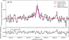 |
Fig. 3 Same as Fig. 2 but for the HC15N line at 344.2003 GHz. |
| In the text | |
|
Fig. 4 Selection of H12C14N vertical profiles used in our radiative-transfer modelling at different latitudes and all (arbitrarily) taken from the eastern limb. They illustrate the limited variety of profiles retrieved at all low-to-mid latitudes on both limbs, as shown in Cavalié et al. (2023). The filled areas show the 1σ envelope resulting from the 1σ uncertainties on the retrieved profile parameters. A typical temperature profile extracted at the equator is also displayed on the top x-axis as an example (dashed black line). The full 3D temperature field can be found in Cavalié et al. (2023). |
| In the text | |
|
Fig. 5 Review of 12C/13C ratio in the various Solar System objects. Detailed information on the instrument, the observation date, and the references are reported in Tables A.1 (giant planets only) and A.2 (the other Solar System determinations) and references therein. |
| In the text | |
|
Fig. 6 Review of 14N/15N ratio in the various Solar System objects. Detailed information on the instrument, the observation date, and the references are reported in Table A.3 and references therein. |
| In the text | |
Current usage metrics show cumulative count of Article Views (full-text article views including HTML views, PDF and ePub downloads, according to the available data) and Abstracts Views on Vision4Press platform.
Data correspond to usage on the plateform after 2015. The current usage metrics is available 48-96 hours after online publication and is updated daily on week days.
Initial download of the metrics may take a while.