| Issue |
A&A
Volume 641, September 2020
|
|
|---|---|---|
| Article Number | A140 | |
| Number of page(s) | 9 | |
| Section | Planets and planetary systems | |
| DOI | https://doi.org/10.1051/0004-6361/202038188 | |
| Published online | 24 September 2020 | |
Monitoring of the evolution of H2O vapor in the stratosphere of Jupiter over an 18-yr period with the Odin space telescope
1
Laboratoire d’Astrophysique de Bordeaux, Univ. Bordeaux, CNRS,
B18N, allée Geoffroy Saint-Hilaire,
33615
Pessac, France
e-mail: This email address is being protected from spambots. You need JavaScript enabled to view it.
2
LESIA,
Observatoire de Paris, Université PSL, CNRS, Sorbonne Université, Univ. Paris Diderot, Sorbonne Paris Cité,
5 place Jules Janssen,
92195
Meudon, France
3
Université Montpellier 2 Sciences et Techniques,
Place E. Bataillon 30,
34095
Montpellier, France
4
Stockholm Observatory, Stockholm University, AlbaNova University Center,
106 91
Stockholm, Sweden
5
Southwest Research Institute,
San Antonio,
TX
78228, USA
6
Max Planck Institut für Sonnensystemforschung,
Justus-von-Liebig-Weg 3,
37077
Göttingen, Germany
7
Department of Earth and Space Sciences, Chalmers University of Technology, Onsala Space Observatory,
439 92, Onsala, Sweden
8
Omnisys Instruments AB,
Solna Strandväg 78,
171 54,
Solna, Sweden
9
Chalmers University of Technology,
Gothenburg, Sweden
Received:
17
April
2020
Accepted:
8
July
2020
Abstract
Context. The comet Shoemaker-Levy 9 impacted Jupiter in July 1994, leaving its stratosphere with several new species, with water vapor (H2O) among them.
Aims. With the aid of a photochemical model, H2O can be used as a dynamical tracer in the Jovian stratosphere. In this paper, we aim to constrain the vertical eddy diffusion (Kzz) at levels where H2O is present.
Methods. We monitored the H2O disk-averaged emission at 556.936 GHz with the space telescope between 2002 and 2019, covering nearly two decades. We analyzed the data with a combination of 1D photochemical and radiative transfer models to constrain the vertical eddy diffusion in the stratosphere of Jupiter. Results. Odin observations show us that the emission of H2O has an almost linear decrease of about 40% between 2002 and 2019. We can only reproduce our time series if we increase the magnitude of Kzz in the pressure range where H2O diffuses downward from 2002 to 2019, that is, from ~0.2 mbar to ~5 mbar. However, this modified Kzz is incompatible with hydrocarbon observations. We find that even if an allowance is made for the initially large abundances of H2O and CO at the impact latitudes, the photochemical conversion of H2O to CO2 is not sufficient to explain the progressive decline of the H2O line emission, which is suggestive of additional loss mechanisms.
Conclusions. The Kzz we derived from the Odin observations of H2O can only be viewed as an upper limit in the ~0.2 mbar to ~5 mbar pressure range. The incompatibility between the interpretations made from H2O and hydrocarbon observations probably results from 1D modeling limitations. Meridional variability of H2O, most probably at auroral latitudes, would need to be assessed and compared with that of hydrocarbons to quantify the role of auroral chemistry in the temporal evolution of the H2O abundance since the SL9 impacts. Modeling the temporal evolution of SL9 species with a 2D model would naturally be the next step in this area of study.
Key words: planets and satellites: individual: Jupiter / planets and satellites: atmospheres / submillimeter: planetary systems
© B. Benmahi et al. 2020
 Open Access article, published by EDP Sciences, under the terms of the Creative Commons Attribution License (http://creativecommons.org/licenses/by/4.0), which permits unrestricted use, distribution, and reproduction in any medium, provided the original work is properly cited.
1 Introduction
From the first observations of water (H2O) in the stratospheres of giant planets (Feuchtgruber et al. 1997), the existence of external sources of material to these planets, such as rings, icy satellites, interplanetary dust particles (IDP), and cometary impacts, was demonstrated. Indeed, H2O cannot be transported from the tropospheres to the stratospheres due to a cold trap at the tropopause of all these planets. Regarding the nature of the external sources, it has been shown that Enceladus plays a major role in delivering H2O to Saturn’s stratosphere (Waite et al. 2006; Hansen et al. 2006; Porco et al. 2006; Hartogh et al. 2011; Cavalié et al. 2019), while an ancient comet impact is the favored hypothesis in the case of Neptune for carbon monoxide (CO), hydrogen cyanide (HCN), and carbon monosulfide (CS) (Lellouch et al. 2005, 2010; Hesman et al. 2007; Luszcz-Cook & de Pater 2013; Moreno et al. 2017). For Uranus, the situation remains unclear (Cavalié et al. 2014; Moses & Poppe 2017).
In July 1994, astronomers witnessed the first extraterrestrial comet impact when the Shoemaker-Levy 9 comet (SL9) hit Jupiter. Several fragment impacts were observed around − 44° latitude (Schulz et al. 1995; Sault et al. 1997; Griffith et al. 2004), which delivered several new species, including H2O (Lellouch et al. 1995; Bjoraker et al. 1996). Piecing together several observations of H2O vapor in the infrared and submillimeter with the Infrared Space Observatory (ISO), the Submillimeter Wave Astronomy Satellite (SWAS), Odin and Herschel, it was established that Jupiter’s stratospheric H2O comes from the impact of the SL9 comet (Bergin et al. 2000; Lellouch et al. 2002; Cavalié et al. 2008a, 2012, 2013).
Cavalié et al. (2012) used the monitoring of the H2O emissions to try and constrain the vertical eddy mixing in Jupiter’s stratosphere. Their sample of Odin observations only covered 2002 to 2009 and did not allow them to unambiguously demonstrate that the line emission was decreasing with time, as was expected from the comet impact scenario. Fortunately, the Odin space telescope is still in operation and has continued ever since to regularly monitor the H2O emission from the stratosphere of Jupiter. In this paper, we extend the monitoring presented in Cavalié et al. (2012) by adding new observations from 2010 to 2019, hence doubling the time baseline. While H2O is not as chemically stable as, for example, HCN (Moreno & Marten 2006; Cavalié et al. 2013) and cannot, in principle, be used to constrain horizontal diffusion without a robust chemistry and diffusion model, we assume the oxygen chemistry to be sufficiently well-known after recent progress (Dobrijevic et al. 2014, 2016, 2020; Loison et al. 2017). Thus, we use H2O as a tracer to constrain vertical diffusion in Jupiter’s stratosphere, similarly to HCN, CO, and carbon dioxide (CO2) in Moreno et al. (2003), Griffith et al. (2004), and Lellouch et al. (2002, 2006). Our work therefore assumes H2O has small meridional variability by the time of our first observation in 2002, that is, on the order of that measured by Moreno et al. (2007) in HCN and Cavalié et al. (2013) in H2O (a factor of 2–3). With nearly two decades of data, we can probe the layers from the level where H2O was originally deposited by the comet to its current location by following its downward diffusion with our spectroscopic observations.
We present the Odin observations made between 2002 and 2019 in Sect. 2. We introduce the photochemical and radiative transfer models that we used in this study in Sect. 3. Results of both the photochemical model and the analysis of Odin observations are given in Sect. 4, followed by a discussion on the eddy diffusion profile in Sect. 5. We provide our conclusion in Sect. 6.
2 Observations
Odin (Nordh et al. 2003) is a Swedish-led space telescope of 1.1 m in diameter that was launched into polar orbit in 2001, at an altitude of 600 km. It carries out observations in the submillimeter domain across the frequency bands of 486–04 GHz and 541–581 GHz. The observations of the H2O (110 –101) line at 556.936 GHz in Jupiter’s stratosphere used in this paper were made with the Submillimeter and Millimeter Radiometer (Frisk et al. 2003) and the Acousto-Optical Spectrometer (Lecacheux et al. 1998) using the Dicke switching observation mode. This mode is the standard Odin observation mode (Olberg et al. 2003; Hjalmarson et al. 2003). It enables integrating a target and a reference position on the sky by using a Dicke mirror. This allows us to compensate for short-term gain fluctuations. In addition, a few orbits are integrated on the sky 15′ away from the source to remove other effects that are not corrected by the Dicke switching technique, such as the ripple continuum and continuum spillover from the main beam.
A first monitoring of Jupiter’s stratospheric H2O emission at 557 GHz was already carried out by Odin over the 2002–2009 period (Cavalié et al. 2012). We obtained additional data between 2010 and 2019 for the following dates: 2010/11/20, 2012/02/17, 2012/02/24, 2012/10/05, 2013/03/01, 2013/10/04, 2013/10/27, 2014/04/04,2014/10/17, 2015/04/19, 2016/12/16, 2018/02/02, 2019/02/22, and 2019/10/09. Thus, we double the time coverage of the Odin monitoring. For each observation date, we accumulated, on average, nine orbits of integration time; for the nine orbits we have six (× ~1 h integration) ON Jupiter and three OFF at 15′ to remove the residual background that we get in the Dicke switch scheme. Each observation was reduced with the same method as in Biver et al. (2005) and Cavalié et al. (2012). Residual continuum baselines were removed using a normalized Lomb periodogram (see Fig. 1, top) to produce the baseline-subtracted spectra we analyzed, presented below (see Fig. 1 bottom).
Odin’s primary beam is about 126′′ at 557 GHz, whereas the apparent size of Jupiter is about 35′′ as Odin observes when Jupiter is in quadrature. Thus, we obtained disk-averaged spectra. Even though the temporal evolution of the disk-averaged H2O vertical distribution following the SL9 impacts implies that two different dates should correspond to two different vertical profiles, we chose, whenever possible, to average the observations by groups of two or three that are not too far apart in time to increase the signal-to-noise ratio (S/N). All 2012 observations have been averaged into a single observation and we link this observation to an equivalent date of 2012/05/21 for our modeling. We proceeded similarly with all 2013 observations (equivalent date of 2013/09/08), with the 2014 and 2015 observations (equivalent date of 2014/10/29), with the 2016 and 2018 observations(equivalent date of 2017/07/22), and with the 2019 observations (equivalent date of 2019/06/17). With the initial 2010 and final 2019 observations, we have a total of six new spectra covering 2010-2019. To further increase the S/N, wesmoothed the spectra from their native spectral resolution of 1.1 MHz to 10 MHz. This has a very limited impact on the line shape, given the line is already substantially smeared by the rapid rotation of the planet (12.5 km s−1 at the equator).
The ten spectra that span the 2002–2019 time period which we used in our analysis are shown in Fig. 2. Given the limited sensitivity per spectral channel of our observations, there is very limited vertical information that can be directly retrieved from the line profile. The main information resides in the line area. In addition, the line width is mainly controlled by the rapid rotation of the planet, so that the line amplitude (l) remains the only diagnostic for temporal variability. Because observations were carried out at different Odin–Jupiter distances, there is non-negligible variability in the beam filling factor. To get rid of this variability and keep only the variability caused by the evolution of the water abundance, we divided the spectra by their observed antenna temperature continuum (c) to produce and subsequently analyze line-to-continuum ratio (l/c) spectra. We computed the l/c by averaging the peak of the line over a range of ±5 km s−1 and the continuum excluding the central ±50 km s−1. This has thebenefit of cancelling out the variable beam dilution effect that results from the variable Jupiter-Odin distance from one another date and that impacts similarly the observed line amplitude and continuum. The evolution of the l/c of the Odin observationsbetween 2002 and 2019 is presented in Fig. 3. We note that the long-term stability of Odin’s hot calibrator is better than 2% and is accounted for in the total power calibration scheme. It has no effect on the temporal evolution of the l/c. In addition, any detector sensitivity changes over the course of this monitoring would have similar effects on both continuum and line amplitude. So the temporal evolution seen on the l/c in Fig. 3 is only caused by changes in the H2O abundance.
 |
Fig. 1 Top: example of the 2010 raw observation of H2O in the stratosphere of Jupiter (black solid line) and continuum baseline (red dashed line) removed by using a Lomb periodogram. This observation was the most affected by continuum ripples. Later spectra barely showed any continuum baselines and are not shown here to preserve clarity. Bottom: baseline-subtracted spectra recorded after 2010 and used in this study in complement to the observations of Cavalié et al. (2008a, 2012). |
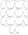 |
Fig. 2 Odin observations of H2O at 556.936GHz in Jupiter’s stratosphere between 2002 and 2019. The spectral resolution is 10 MHz. The blue lines correspond to our nominal temporal evolution model (obtained with Kzz Model B). |
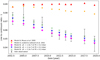 |
Fig. 3 Evolution of the H2O line-to-continuum ratio observed by Odin in the atmosphere of Jupiter (black points). The blue stars represent the results obtained with our Kzz Model B. The green and pink dots correspond to different values of the y0 parameter with the same model. The red triangles stand for our nominal parameters of y0 and p0 and Kzz Model A (profile from Moses et al. 2005). The orange dots depict the results obtained with the vertical profiles of Model A after rescaling their respective column densities to the temporal evolution modeled by Lellouch et al. (2002) with their chemistry-2D transport model. |
3 Models
In this section, we present the models used to reproduce the decrease in the H2O l/c at 557 GHz observed by the Odin space telescope between 2002 and 2019. These calculations were carried out with a 1D time-dependent photochemical model to simulate the H2O disk-averaged mole fraction vertical profile in the atmosphere of Jupiter after the SL9 impact at each observation date, and a radiative transfer code to simulate the Odin spectra. We first present the photochemical model, then the radiative transfer model, and, finally, our modeling strategy.
3.1 Photochemical model
The 1D time-dependent photochemical model used in the present study is adapted from the recent model developed for Neptune by Dobrijevic et al. (2020), which couples ion and neutral hydrocarbon and oxygen species. The ion-neutral chemical scheme remains unchanged (see Dobrijevic et al. 2020 for details). In the following sections, we only outline the parameters specific to Jupiter usedin this model.
3.1.1 Boundary conditions
In the first step of the 1D photochemical modeling, we assumed a background flux of H2O, CO, and CO2 supplied by a constant flux of IDP with influx rates Φi at the top boundary given by Moses & Poppe (2017):  cm−2 s−1,
  ,
,  . We also account for the internal source of CO with a tropospheric mole fraction of 1 ppm (Bézard et al. 2002). Unlike previous photochemical models, we did not include a downward flux of atomic hydrogen at the upper boundary to account for additional photochemical production of H in the higher atmosphere. We assumed that photo-ionization and subsequent ionic chemistry were responsible for this source previously added to the models. All other species were assumed to have zero-flux boundary conditions at the top of the model atmosphere (corresponding to a pressure of about 10−6 mbar).
At the lower boundary (1 bar), we set the mole fraction of He, CH4, and H2, respectively, to yHe = 0.136,  , and
, and  (see Hue et al. 2018 for details). All other compounds have a downward flux given by the maximum diffusion velocity v = Kzz∕H where Kzz is the eddy diffusion coefficient and H the atmospheric scale height at the lower boundary.
3.1.2 Temperature and vertical transport
The pressure-temperature profile used in the present study for all observation dates is shown in Fig. 4. Details on this profile can be found in Hue et al. (2018). We chose to use this disk-averaged temperature profile throughout the 18-yr observation period of Odin because Jupiter barely shows disk-averaged seasonal variability (Hue et al. 2018). In addition, Cavalié et al. (2012) already showed that reasonable disk-averaged stratospheric temperature variations could not explain the H2O l/c evolution in the 2002–2009 period. Since the l/c decrease has continued ever since, the disk-averaged stratospheric temperature would have had to drop continuously by ≥10 K over the 2002–2019 period. Even though such variability can be seen locally, such disk-averaged variability is contradicted by observations(Greathouse et al. 2016).
Our baseline Kzz eddy diffusion profile (Model A in what follows) is the Model C of Moses et al. (2005). This profile ensures having a CH4 mole fraction profile in agreement with observations of Greathouse et al. (2010) around the homopause. To fit the temporal evolution of the H2O emission seen by Odin, we had to adjust this profile in the pressure range probed by the H2O line. More details are given in Sect. 3.3. The resulting eddy profile (Model B hereafter) shown in Fig. 4 and has a simple expression given by:  , where Kref = 4.5 × 105 cm2 s−1, pref = 10−2 mbar, and a = 0.4 if p(z) < pref and a = 0.469 otherwise.
3.2 Radiative transfer model
We applied the radiative transfer model described in Cavalié et al. (2008b, 2019) and used the temperature profile as well as the output mole fraction profiles of the photochemical model. Both are therefore applied uniformly in latitude and longitude over the Jovian disk.
Details regarding the Jovian continuum opacity, spectroscopic data, and the effect of Jovian rapid rotation can be found in Cavalié et al. (2008a). We adopt the following broadening parameters (pressure-broadening coefficient γ and its temperature dependence n) for H2O, NH3 and PH3 :  0.080 cm−1 atm−1,
  ,
,  cm−1 atm−1,
  0.73,
0.73,  cm−1 atm−1, and
  (Dick et al. 2009; Fletcher et al. 2007; Levy et al. 1993, 1994). The final spectra are smoothed to a resolution of 10 MHz.
Odin’s pointing has been checked twice a year and has remained stable within a few arcsec since its launch. However, larger pointing errors can occur when Odin is pointing to Jupiter close to occultation by the Earth (i.e., at the beginning and at the end of observations during an orbit). Only one star-tracker can then be used for the platform pointing stability, the other one pointing at the Earth. It results in a significant decrease of the pointing performance. For each Odin observation, we therefore used radiative transfer simulations to fit any east-west pointing error. Despite the large Odin beam-size with respect to the size of Jupiter, an east-west pointing error will slightly modify the weights of the various emission regions of the rotating planet during the beam convolution, and blue-shift the line if there is an eastward pointing error or red-shift the line if there is an westward pointing error. The offsets we found are: +15.6′′ for 2002.86, −34′′ for 2005.09, +8′′ for 2007.16, −6′′ for 2008.90, −5′′ for 2010.90, −16′′ for 2012.40, +5′′ for 2013.62, +8′′ for 2014.83, +51′′ for 2017.56, and +20′′ for 2019.46. The vast majority of values remain smaller than one fifth of the beam size. The 2017.56 spectrum, which has the largest pointing error, is also unsurprisingly the one with the lowest quality fit. The pointing offset also marginally affects the l/c and can be best seen in the results obtained using the Moses et al. (2005) eddy mixing profile (red triangle in Fig. 3), where some small jumps in the l/c are present (e.g., compare the 2017 point to thesurrounding 2014 and 2019 points). The l/c is also affected, in principle, by north–south pointing errors, especially if the thermal field is not meridionally uniform. However, we have no means to constrain such an error.
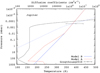 |
Fig. 4 Temperature–pressure profile taken from Hue et al. (2018; black solid line). Eddy diffusion coefficient Kzz profile from Moses et al. (2005; red solid line – Model A) compared to our nominal profile (blue solid line – Model B). The CH4 homopause occurs where the Kzz profile crosses the CH4 molecular diffusion coefficient profile (blue dashed lines). The Kzz value derived by Greathouse et al. (2010) at this level is shown for comparison. Our nominal Kzz is unconstrained from our H2O observationsfor pressures higher than ~5 mbar. |
3.3 Modeling procedure
The photochemical model was used in two subsequent steps for a given Kzz profile. First, we ran our model with the background oxygen flux until the steady state was reached for all the species. The results of this steady state1 then served as a baseline for the second step of the modeling.
In this second step, we treated the cometary impact in a classical way (Moreno et al. 2003; Cavalié et al. 2008a). We considered a sporadic cometary supply of H2O in July 1994 with two parameters: the initial mole fraction of H2O y0 deposited above a pressure level p0. This level was measured, for example, by Moreno et al. (2003) and found to be 0.2 ± 0.1 mbar. We thus fixed p0 to 0.2 mbar in our study. The value of y0 was then found by chi-square minimization and was usually close to the values reported by Cavalié et al. (2008a, 2012). We also added a CO component with a constant mole fraction of 2.5 × 10⁻⁶ for p < p0 at the start of our simulations, in agreement with Bézard et al. (2002) and Lellouch et al. (2002), to account for the H2O–CO chemistry. The model was then run for integration times corresponding to the time intervals between the comet impacts and the Odin observation dates. The abundance profiles were extracted for each Odin observation date. We then simulated the H2O line at 556.936 GHz line for each date and compared the resulting spectra with the observations by using the χ2 method. We started with the Kzz Model A and adjusted it subsequently to obtain Model B by cycling the whole procedure until a good fit of all the H2O lines was obtained.
4 Results
Figure 3 shows that the decrease of the l/c, which was only hinted in the first half of the monitoring (Cavalié et al. 2012) and was eventually demonstrated, with a decrease of ~40% between 2002 and 2019. This provides evidence that the vertical profile of H2O has evolved over this time range and we thus used it to constrain vertical transport from our modeling.
We first estimated the level of the residence of H2O as a function of time with forward radiative transfer simulations using parametrized vertical profiles in which the H2O mole fraction is set constant above a cut-off pressure level. Despite the limited S/N of our observations, we were able to estimate these levels as a function of time. The most noticeable result is that we see the downward diffusion of H2O as the cut-off level evolves from ~0.2 mbar to ~5 mbar over the 2002–2019 monitoring period. This is the pressure range in which we could constrain Kzz.
For each Kzz profile we tested, we explored a range of y0 values (with p0 always fixed to 0.2 mbar) and generated the H2O vertical profile for each Odin observation between 2002 and 2019. We then compared the lines resulting from these profiles with the observations in terms of l/c, and searched for acceptable fits (using a reduced χ2 test) of the temporal evolution of the H2O l/c at 557 GHz. The best-fit values of y0 were usuallyfound close to the values of Cavalié et al. (2008a, 2012), which were in agreement with previous ISO observations (Lellouch et al. 2002).
We first noted that there is no (y0,p0) combination that enables fitting the Odin l/c for all dates when using the Kzz profile derived by Moses et al. (2005) (our Model A), even though main hydrocarbon observations2 were reproduced (see Fig. 5). The red points in Fig. 3 show, for instance, the results obtained using our nominal parameters for y0 and p0 (see below).In the first years after the impacts, we find that a small fraction of H2O (and CO) is converted into CO2, as shown by Lellouch et al. (2002) and also previously found by Moses (1996) for impact sites. The main difference between the two studies is that our model is a 1D, globally-averaged model with complete and up-to-date chemistry, while in their study of the evolution of H2O and CO2, Lellouch et al. (2002) used a simplified chemistry model along with a latitude-dependent model describing the spatial evolution of the SL9-generated compounds due to meridional eddy mixing. The initial disk-averaged H2O and CO abundances are, thus, lower in our Model A than those in the narrow latitudinal band in Lellouch et al. (2002). This is also true for our Model B (see hereafter). Given our assumed initial CO and H2O values, we find a loss of 5% of the H2O column between the time of impact and 2019 and of only 1% between 2002 and 2019 (see Fig. 6), which does not translate into a proportional decrease of the spectral line l/c.
We note, however, that the loss in the first years following the impacts is likely to be underestimated in this model (and so would the production of CO2) because the H2O and CO abundances were ~10 times higherin the latitudes around the impacts (Lellouch et al. 2002). A simple 1D simulation with such abundances (Model A′, initial CO mole fraction of 2.5 × 10⁻⁵ above 0.2 mbar, i.e., ten times more than in Model A) until 1997 (i.e., the date of the ISO observations of Lellouch et al. 2002) leads to a loss of 31% of the H2O column (vs. only 3% in Model A). However, even if the initial loss is indeed underestimated in our Model A, the slope of the l/c between 2002 and 2019 would not be significantly altered between Model A and a model that would start with the conditions of Model A′ and continue with disk-averaged abundances at the start of our Odin campaign (still assuming that the factor of 2–3 horizontal variability seen in H2O in 2009 by Cavalié et al. 2013 is small enough that it can be neglected). The slope might even be flatter given that more H2O would have been consumed in the first place. After 2002, the loss of H2O would then be even slower. Actually, if we take the vertical profiles of Model A and scale their respective column densities to match the temporal evolution of the chemistry-2D transport model of Lellouch et al. (2002; from their Fig. 12), we find an intermediate case shown in Fig. 3. However, this model falls short by a factor of four to reproduce the temporal decrease of the l/c observed between 2002 and 2019, as it only produces a decrease of the l/c of ~10%.
By increasing the magnitude of Kzz in the millibar and submillibar pressure ranges, for instance from 1.4 × 104 cm2 s−1 to 5.2 × 104 cm2 s−1 at 1 mbar and from 7.8 × 104 cm2 s−1 to 1.5 × 105 cm2 s−1 at 0.1 mbar, we could accelerate the decrease of the l/c to before the start of the Odin monitoring. With this Kzz Model B, shown in Fig. 4, we were able to fit the pattern of the l/c temporal evolution within error bars. Figure 3 shows our best results (green crosses, blue squares, and pink stars). These results show that the initial disk-averaged H2O mole fraction deposited by SL9 above the 0.2 mbar pressure level was likely in the range [y0 = 1.0 × 10⁻⁷, y0 = 1.2 × 10⁻⁷]. In Model B, we find that the column of CO2 tops at 0.1% of the total O column (which again must be underestimated) and starts decreasing after 2 × 10⁸ s (~6 yr after the impacts), when the production of CO2 by the CO+OH reaction becomes lessefficient than CO2 photolysis. The production and loss mechanisms for oxygen species as of 2019 are summarized in Fig. 7. It essentially shows that H2O is efficiently recycled and is only lost due to condensation. CO2 is lost to CO and H2O via photolysis. The evolution of the H2O abundance profile according to our Model B (with y0 = 1.1 × 10⁻⁷ above a pressure level p0 = 0.2 mbar) is shown in Fig. 8 at the time of the SL9 impacts and of each Odin observation. We also show a prediction for 2030 when JUICE (Jupiter Icy Moons Explorer) will start observing Jupiter’s atmosphere. We note that the simulation gives us a decrease of the H2O abundance as a function of time for pressures lower than ~5 mbar between 2002 and 2019, while it tends to increase at higher pressures because of vertical mixing.
We finally verified the agreement of Model B at the steady state for the main hydrocarbons. Figure 5 (top) shows that our CH4 profile remains in good agreement with the Greathouse et al. (2010) observations, which is not surprising since model A and B share a common homopause. However, the C2H6 profile (Fig. 5 bottom) is incompatible with the observations, questioning the validity of Kzz Model B. This profile is not a unique solution and properly deriving the error bars on its vertical profile would require a full retrieval, which is beyond the scope of this paper. However, we performed several tests to look for other (Kzz, y0, p0) combinations to explain the observed l/c evolution and found our Kzz Model B tobe quite robust as there is no solution that enables fitting both the H2O temporal evolution and the hydrocarbon vertical profiles simultaneously. There is, thus, a contradiction between the Odin H2O monitoring observations and the hydrocarbon observations in terms of vertical mixing when interpreted with a 1D time-dependent photochemical model.
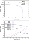 |
Fig. 5 Top: mole fraction profiles of CH4 using the Kzz Models A (red line) and B (blue line). Observations of Greathouse et al. (2010) are given for comparison. Bottom: mole fraction profiles of C2H2, C2H4, and C2H6 (same layout). Several observations are given for comparison (see Moses & Poppe 2017 for details). |
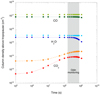 |
Fig. 6 Column densities as a function of time after the SL9 impacts (1994) for CO, H2O, and CO2. Model A results in the light green, cyan, and orange curves, while Model B results in the dark green, dark blue, and red ones. The offset between the two models results from the different background column resulting from the IDP source (see Sect. 3.1.1). The period covering the Odin monitoring (2002-2019) is highlighted in grey. |
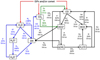 |
Fig. 7 Simple schematic of the chemical network of oxygen species based on integrated chemical loss term over altitude. This illustrates the fate of oxygen species from the external input (IDPs or comet) of H2O, CO, and CO2 in the atmosphere of Jupiter. For each species, the main loss processes are given. Photolysis is represented by hν and for reactions, the other reactant is given as a label. The percentage of the total integrated loss term over altitude is given with the altitude at which this process is at maximum. Blue: sub-chemical scheme of H2O-related species. Black: sub-chemical scheme of CO-related species. Green: sub-chemical scheme of CO2 -related species. Percentages change slightly depending on the amount of water in the atmosphere (i.e., before and after the comet impact), but the whole scheme stays the same. Values given here correspond to the state of the chemistry just after the influx of H2O due to the impact. |
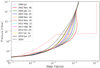 |
Fig. 8 Evolution of the H2O abundance profile in the stratosphere of Jupiter for y0 = 1.1 × 10⁻⁷ above a pressure level p0 = 0.2 mbar (SL9 parameters) and Kzz Model B. These profiles are obtained from the photochemical model and a comparison with the observations. The red dotted abundance profile represents the initial profile of H2O at the time of the SL9 comet impacts in 1994. Each solid curve represents the abundance profile of H2O at dates corresponding to Odin observations. The black dashed profile represents the abundance of H2O that we predict for 2030. |
5 Discussion
In a 1D photochemical model, vertical transport is dominated by molecular diffusion at altitudes above the homopause and eddy mixing below this limit. The Kzz profile is a free parameter of 1D photochemical models. The best way to constrain this parameter is to compare the model results with the observational data of a particular species. In the case of Titan, an inert species like argon (Ar) is very useful for this purpose. For the giant planets, the situation is more complex. The homopause can be constrained using CH4 observationsin the upper atmosphere since its profile is driven by molecular diffusion. Below the homopause, the Kzz profile is usually constrained from a comparison between observations and model results for the main hydrocarbons (C2H2 and C2H6). Unfortunately, this is an imprecise methodology since model results have strong uncertainties (see, for instance, Dobrijevic et al. 2010 for Neptune and Dobrijevic et al. 2011 for Saturn), which can be much larger than uncertainties on observational data. In a recent photochemical model of Titan, Loison et al. (2019) used H2O and HCN to constrain Kzz in the lower stratosphere. One of the reasons for this is that the chemical processes that drive their abundances are expected to be simpler than those for hydrocarbons and the model uncertainties caused by chemical rates are, therefore, more limited. In the case of Neptune, Dobrijevic et al. (2020) showed that uncertainties on model results for H2O are very low compared to other oxygen species and hydrocarbons; therefore, this species is currently the best tracer of the vertical diffusion in the stratosphere of Neptune, assuming its chemistry is well-known. In the present paper, we assume that this is also the case for Jupiter (and the other giant planets).
The delivery of H2O, among other species such as HCN, CO, and carbon sulfide (CS) to Jupiter’s stratosphere by comet SL9 in 1994 (Lellouch et al. 1995) further enhances the interest of using these species as tracers for horizontal and vertical dynamics in this atmosphere, provided that either they are chemically stable over the time considered or their chemistry is properly modeled. For instance, Moreno et al. (2003), Griffith et al. (2004) and Lellouch et al. (2006) used HCN, CO, and CO2 to constrain longitudinal and mostly meridional diffusion in the years following the impacts, even though CO2 is not chemically stable (Lellouch et al. 2002). In the present study, we use nearly two decades of H2O disk-averaged emission monitoring with Odin and a 1D photochemical model to constrain vertical diffusion in Jupiter’s stratosphere. Not only does the modeling of the H2O vertical profile suffer less from chemical rate uncertainties than hydrocarbons (Dobrijevic et al. 2020), but the progressive downward diffusion of H2O from its initial deposition level (p0 in our model) enabled us to probe Kzz at various altitudes as a function of time. This will remain true for the years to come, until the bulk of H2O eventually reaches its condensation level at ~30 mbar.
When assuming Model A for Kzz, we cannot fit the ~40% decrease observed on the l/c, even if we find a global decrease of the H2O column of 5% between the impacts and 2019. The H2O is too efficiently recycled for its profiles to reproduce the time series of Odin observations. We can only fit this time series with the 1D model if we alter Kzz to that of Model B. While the initial loss ofH2O is caused by the build-up of the CO2 column, condensation becomes the main loss factor after ~2 × 10⁸ s (about 6 yr after the impacts) and enables the fitting of the H2O observations. The CO2 also starts to be lost to H2O and the subsequent condensation of H2O.
While the Odin time series of H2O observations can be fitted with our 1D model and Kzz Model B, the resulting C2Hx profiles are inconsistent with numerous observations, even when accounting for the joint error bar of the observationsand the photochemical model itself. This tends to demonstrate that our 1D model cannot fit jointly C2Hx and the H2O observation time series. The Kzz Model A probably remains the best disk-averaged estimate of Kzz in Jupiter’s stratosphere. In this context, Model B can only be seen as an upper limit. The H2O must then have an additional loss process.
We offer a promising approach to explore the auroral regions of Jupiter as the regions of enhanced loss of H2O by means of ion-neutral chemistry. Dobrijevic et al. (2020) showed that ion-neutral chemistry affected the abundances of oxygen species in Neptune’s atmosphere, even without including magnetospheric ions and electrons. With energetic electrons precipitating down to the submillibar level under Jupiter’s aurorae (Gérard et al. 2014), ion-neutral chemistry could be the cause for an enhanced loss of H2O, possibly producing excess CO2. This could explain the peak in the CO2 meridional distribution seen 6 yr after the SL9 impacts only at the south pole by Lellouch et al. (2006), as SL9-originating CO and H2O had not yet reached the northern polar region (Moreno et al. 2003; Cavalié et al. 2013). It should be noted that unexpected distributions of hydrocarbons have already been found in Jupiter’s auroral regions. Kunde et al. (2004) and Nixon et al. (2007) found that, unlike C2H2, the zonal mean of C2H6 did not follow the mean insolation and peaked at polar latitudes. Hue et al. (2018) demonstrated that this discrepancy between two species that share a similar neutral chemistry cannot be explained either by neutral chemistry or by a combination of advective and diffusive transport. In turn, they proposed ion-neutral chemistry in the auroral region as a mechanism for bringing the zonal mean of C2H6 out of equilibrium with the solar insolation. More recently, Sinclair et al. (2018) measured the longitudinal variability of the main C2Hx species at northern and southern auroral latitudes. They found that C2H2 and C2H4 were significantly enhanced at millibar and submillibar pressures under the aurora, while C2H6 remained fairly constant. In addition, Sinclair et al. (2019) found that heavier hydrocarbons like C6 H6 were also enhanced under the aurorae. This points to a richer chemistry than that seen at lower latitudes, increasing the production of several hydrocarbons and ultimately producing Jupiter’s aerosols (Zhang et al. 2013, 2016; Giles et al. 2019). Such a richer chemistry could also apply to H2O and other oxygen species. At this point, however, this remains speculative and requires modeling the auroral chemistry under Jovian conditions with and without SL9 material.
6 Conclusion
In this paper, we present disk-averaged observations of H2O vapor in thestratosphere of Jupiter carried out with the Odin space telescope. This temporal monitoring of the H2O line at 557 GHz spans over nearly two decades, starting in 2002, that is, 8 yr after its delivery by the comet SL9. We demonstrate that the line-to-continuum ratio has been decreasing as a function of time by ~40% over this period. Such a trend results from the evolution of the H2O disk-averaged vertical profile and we used it to study the chemistry and dynamics of the Jovian atmosphere.
We thus used our observations to constrain Kzz in the levels where H2O resided at the time of our observations, that is, between ~0.2 and ~5 mbar. Using a combination of photochemical and radiative transfer modeling, we showed that the Kzz profile of Moses et al. (2005) could not reproduce the observations. We had to increase the magnitude of Kzz by a factor of ~2 at 0.1 mbar and ~4 at 1 mbar tofit the full set of Odin observations.
However, this Kzz profile makes the C2H6 profile fall outside observational and photochemical model error bars and is thus not acceptable. As a result, 1D time-dependent photochemical models cannot reproduce both the main hydrocarbon profiles and the temporal evolution of the disk-averaged H2O vertical profile. A possible explanation is that these species still vary locally more sharply as a function of latitude than the factor of two to three indicated by the low spatial resolution observations of Cavalié et al. (2013); we note that these variations cannot be studied with 1D models, by definition. Sinclair et al. (2018, 2019) already demonstrated that the auroral regions of Jupiter harbor chemistry influencing the hydrocarbons that is not seen elsewhere on the planet. The same may be also be true for H2O, but disk-resolved observations with more resolution than with Herschel (2009–2010) would be required to test this hypothesis, possibly with the James Webb Space Telescope Norwood et al. (2016). In the meantime, the continued monitoring of the Jovian stratospheric H2O emission with Odin will help prepare for future observations to be carried out by the Jupiter Icy Moons Explorer (JUICE).
The study presented in this paper will help to prepare the JUICE mission that is aimed at studying Jupiter and its moons in the 2030s. One instrument of its payload, the Submillimeter Wave Instrument (SWI; Hartogh et al. 2013) will observe the same H2O line as the one observed by Odin to map the zonal winds in the stratosphere of Jupiter from high-resolution spectroscopy at high-spatial resolution. The continuation of the Odin monitoring is, thus, crucial for refining our estimates of the H2O abundance and vertical profile for the 2030s and for optimizing the SWI observation program.
Acknowledgments
This work was supported by the Programme National de Planétologie (PNP) of CNRS/INSU and by CNES. Odin is a Swedish-led satellite project funded jointly by the Swedish National Space Board (SNSB), the Canadian Space Agency (CSA), the National Technology Agency of Finland (Tekes), the Centre National d’Études Spatiales (CNES), France and the European Space Agency (ESA). The former Space division of the Swedish Space Corporation, today OHB Sweden, is the prime contractor, also responsible for Odin operations.
References
- Bergin, E. A., Lellouch, E., Harwit, M., et al. 2000, ApJ, 539, L147 [NASA ADS] [CrossRef] [Google Scholar]
- Bézard, B., Lellouch, E., Strobel, D., Maillard, J.-P., & Drossart, P. 2002, Icarus, 159, 95 [NASA ADS] [CrossRef] [Google Scholar]
- Biver, N., Lecacheux, A., Encrenaz, T., et al. 2005, A&A, 435, 765 [CrossRef] [EDP Sciences] [Google Scholar]
- Bjoraker, G. L., Stolovy, S. R., Herter, T. L., Gull, G. E., & Pirger, B. E. 1996, Icarus, 121, 411 [NASA ADS] [CrossRef] [Google Scholar]
- Cavalié, T., Billebaud, F., Biver, N., et al. 2008a, Planet. Space Sci., 56, 1573 [NASA ADS] [CrossRef] [Google Scholar]
- Cavalié, T., Billebaud, F., Fouchet, T., et al. 2008b, A&A, 484, 555 [NASA ADS] [CrossRef] [EDP Sciences] [Google Scholar]
- Cavalié, T., Biver, N., Hartogh, P., et al. 2012, Planet. Space Sci., 61, 3 [NASA ADS] [CrossRef] [Google Scholar]
- Cavalié, T., Feuchtgruber, H., Lellouch, E., et al. 2013, A&A, 553, A21 [NASA ADS] [CrossRef] [EDP Sciences] [Google Scholar]
- Cavalié, T., Moreno, R., Lellouch, E., et al. 2014, A&A, 562, A33 [NASA ADS] [CrossRef] [EDP Sciences] [Google Scholar]
- Cavalié, T., Hue, V., Hartogh, P., et al. 2019, A&A, 630, A87 [CrossRef] [EDP Sciences] [Google Scholar]
- Dick, M. J., Drouin, B. J., & Pearson, J. C. 2009, J. Quant. Spec. Rad. Transf., 110, 619 [NASA ADS] [CrossRef] [Google Scholar]
- Dobrijevic, M., Cavalié, T., Hébrard, E., et al. 2010, Planet. Space Sci., 58, 1555 [NASA ADS] [CrossRef] [Google Scholar]
- Dobrijevic, M., Cavalié, T., & Billebaud, F. 2011, Icarus, 214, 275 [NASA ADS] [CrossRef] [Google Scholar]
- Dobrijevic, M., Hébrard, E., Loison, J. C., & Hickson, K. M. 2014, Icarus, 228, 324 [NASA ADS] [CrossRef] [Google Scholar]
- Dobrijevic, M., Loison, J. C., Hickson, K. M., & Gronoff, G. 2016, Icarus, 268, 313 [NASA ADS] [CrossRef] [Google Scholar]
- Dobrijevic, M., Loison, J. C., Hue, V., Cavalié, T., & Hickson, K. M. 2020, Icarus, 335, 113375 [CrossRef] [Google Scholar]
- Feuchtgruber, H., Lellouch, E., de Graauw, T., et al. 1997, Nature, 389, 159 [NASA ADS] [CrossRef] [PubMed] [Google Scholar]
- Fletcher, L. N., Irwin, P. G. J., Teanby, N. A., et al. 2007, Icarus, 188, 72 [NASA ADS] [CrossRef] [Google Scholar]
- Frisk, U., Hagström, M., Ala-Laurinaho, J., et al. 2003, A&A, 402, L27 [NASA ADS] [CrossRef] [EDP Sciences] [Google Scholar]
- Gérard, J. C., Bonfond, B., Grodent, D., et al. 2014, J. Geophys. Res., 119, 9072 [NASA ADS] [CrossRef] [Google Scholar]
- Giles, R., Gladstone, R., Greathouse, T. K., et al. 2019, in AGU Fall Meeting Abstracts, Vol. 2019, P21G–3451 [Google Scholar]
- Greathouse, T. K., Gladstone, G. R., Moses, J. I., et al. 2010, Icarus, 208, 293 [NASA ADS] [CrossRef] [Google Scholar]
- Greathouse, T. K., Orton, G. S., Cosentino, R., et al. 2016, in AAS/Division for Planetary Sciences Meeting Abstracts #48, AAS/Division for Planetary Sciences Meeting Abstracts, 501.05 [Google Scholar]
- Griffith, C. A., Bézard, B., Greathouse, T., et al. 2004, Icarus, 170, 58 [NASA ADS] [CrossRef] [Google Scholar]
- Hansen, C. J., Esposito, L., Stewart, A. I. F., et al. 2006, Science, 311, 1422 [NASA ADS] [CrossRef] [PubMed] [Google Scholar]
- Hartogh, P., Lellouch, E., Moreno, R., et al. 2011, A&A, 532, L2 [NASA ADS] [CrossRef] [EDP Sciences] [Google Scholar]
- Hartogh, P., Barabash, S., Beaudin, G., et al. 2013, in European Planetary Science Congress, EPSC2013-710 [Google Scholar]
- Hesman, B. E., Davis, G. R., Matthews, H. E., & Orton, G. S. 2007, Icarus, 186, 342 [NASA ADS] [CrossRef] [Google Scholar]
- Hjalmarson, Å, Frisk, U., Olberg, M., et al. 2003, A&A, 402, L39 [NASA ADS] [CrossRef] [EDP Sciences] [Google Scholar]
- Hue, V., Hersant, F., Cavalié, T., Dobrijevic, M., & Sinclair, J. A. 2018, Icarus, 307, 106 [NASA ADS] [CrossRef] [Google Scholar]
- Kunde, V. G., Flasar, F. M., Jennings, D. E., et al. 2004, Science, 305, 1582 [CrossRef] [Google Scholar]
- Lecacheux, A., Rosolen, C., Michet, D., Clerc, V. 1998, Space-qualified wideband and ultrawideband acousto-optical spectrometers for millimeter and submillimeter radio astronomy. Advanced Technology MMW, Radio, and Terahertz Telescopes, 519 [Google Scholar]
- Lellouch, E., Paubert, G., Moreno, R., et al. 1995, Nature, 373, 592 [Google Scholar]
- Lellouch, E., Bézard, B., Moses, J. I., et al. 2002, Icarus, 159, 112 [Google Scholar]
- Lellouch, E., Moreno, R., & Paubert, G. 2005, A&A, 430, L37 [NASA ADS] [CrossRef] [EDP Sciences] [Google Scholar]
- Lellouch, E., Bézard, B., Strobel, D. F., et al. 2006, Icarus, 184, 478 [Google Scholar]
- Lellouch, E., Hartogh, P., Feuchtgruber, H., et al. 2010, A&A, 518, L152 [NASA ADS] [CrossRef] [EDP Sciences] [Google Scholar]
- Levy, A., Lacome, N., & Tarrago, G. 1993, J. Mol. Spectr., 157, 172 [Google Scholar]
- Levy, A., Lacome, N., & Tarrago, G. 1994, J. Mol. Spectr., 166, 20 [Google Scholar]
- Loison, J. C., Dobrijevic, M., Hickson, K. M., & Heays, A. N. 2017, Icarus, 291, 17 [CrossRef] [Google Scholar]
- Loison, J. C., Dobrijevic, M., & Hickson, K. M. 2019, Icarus, 329, 55 [CrossRef] [Google Scholar]
- Luszcz-Cook, S. H., & de Pater, I. 2013, Icarus, 222, 379 [Google Scholar]
- Moreno, R., & Marten, A. 2006, in AAS/Division for Planetary Sciences Meeting Abstracts #38, AAS/Division for Planetary Sciences Meeting Abstracts, 11.13 [Google Scholar]
- Moreno, R., Marten, A., Matthews, H. E., & Biraud, Y. 2003, Planet. Space Sci., 51, 591 [Google Scholar]
- Moreno, R., Gurwell, M., Marten, A., & Lellouch, E. 2007, in AAS/Division for Planetary Sciences Meeting Abstracts #39, AAS/Division for Planetary Sciences Meeting Abstracts, 9.01 [Google Scholar]
- Moreno, R., Lellouch, E., Cavalié, T., & Moullet, A. 2017, A&A, 608, L5 [NASA ADS] [CrossRef] [EDP Sciences] [Google Scholar]
- Moses, J. I. 1996, in IAU Colloq 156: The Collision of Comet Shoemaker-Levy 9 and Jupiter, eds. K. S. Noll, H. A. Weaver, & P. D. Feldman, 243 [Google Scholar]
- Moses, J. I., & Poppe, A. R. 2017, in AAS/Division for Planetary Sciences Meeting Abstracts #49, AAS/Division for Planetary Sciences Meeting Abstracts, 209.06 [Google Scholar]
- Moses, J. I., Fouchet, T., Bézard, B., et al. 2005, J. Geophys. Res., 110, 8001 [NASA ADS] [CrossRef] [Google Scholar]
- Nixon, C. A., Achterberg, R. K., Conrath, B. J., et al. 2007, Icarus, 188, 47 [NASA ADS] [CrossRef] [Google Scholar]
- Nordh, H. L., von Schéele, F., Frisk, U., et al. 2003, A&A, 402, L21 [NASA ADS] [CrossRef] [EDP Sciences] [Google Scholar]
- Norwood, J., Moses, J., Fletcher, L. N., et al. 2016, PASP, 128, 018005 [Google Scholar]
- Olberg, M., Frisk, U., Lecacheux, A., et al. 2003, A&A, 402, L35 [NASA ADS] [CrossRef] [EDP Sciences] [Google Scholar]
- Porco, C. C., Helfenstein, P., Thomas, P. C., et al. 2006, Science, 311, 1393 [Google Scholar]
- Sault, R. J., Leblanc, Y., & Dulk, G. A. 1997, Geophys. Res. Lett., 24, 2395 [NASA ADS] [CrossRef] [Google Scholar]
- Schulz, R., Encrenaz, T., Stüwe, J. A., & Wiedemann, G. 1995, Geophys. Res. Lett., 22, 2421 [CrossRef] [Google Scholar]
- Sinclair, J. A., Orton, G. S., Greathouse, T. K., et al. 2018, Icarus, 300, 305 [CrossRef] [Google Scholar]
- Sinclair, J. A., Moses, J. I., Hue, V., et al. 2019, Icarus, 328, 176 [CrossRef] [Google Scholar]
- Waite, J. H., Combi, M. R., Ip, W.-H., et al. 2006, Science, 311, 1419 [NASA ADS] [CrossRef] [PubMed] [Google Scholar]
- Zhang, X., West, R. A., Banfield, D., & Yung, Y. L. 2013, Icarus, 226, 159 [NASA ADS] [CrossRef] [Google Scholar]
- Zhang, X., West, R. A., Banfield, D., & Yung, Y. L. 2016, Icarus, 266, 433 [CrossRef] [Google Scholar]
A model with only neutral chemistry was also run to study the effect of the ionic chemistry on the photochemistry of Jupiter and to confirm what Dobrijevic et al. (2020) found for Neptune. Indeed, the ion-neutral coupling affects the production of many species in Neptune’s atmosphere. In particular, it increases the production of aromatics and strongly affects the chemistry of oxygen species. We find similar effects in Jupiter.
Results for the other species are not depicted in the paper, but can be obtained upon request.
All Figures
|
Fig. 1 Top: example of the 2010 raw observation of H2O in the stratosphere of Jupiter (black solid line) and continuum baseline (red dashed line) removed by using a Lomb periodogram. This observation was the most affected by continuum ripples. Later spectra barely showed any continuum baselines and are not shown here to preserve clarity. Bottom: baseline-subtracted spectra recorded after 2010 and used in this study in complement to the observations of Cavalié et al. (2008a, 2012). |
| In the text | |
|
Fig. 2 Odin observations of H2O at 556.936GHz in Jupiter’s stratosphere between 2002 and 2019. The spectral resolution is 10 MHz. The blue lines correspond to our nominal temporal evolution model (obtained with Kzz Model B). |
| In the text | |
|
Fig. 3 Evolution of the H2O line-to-continuum ratio observed by Odin in the atmosphere of Jupiter (black points). The blue stars represent the results obtained with our Kzz Model B. The green and pink dots correspond to different values of the y0 parameter with the same model. The red triangles stand for our nominal parameters of y0 and p0 and Kzz Model A (profile from Moses et al. 2005). The orange dots depict the results obtained with the vertical profiles of Model A after rescaling their respective column densities to the temporal evolution modeled by Lellouch et al. (2002) with their chemistry-2D transport model. |
| In the text | |
|
Fig. 4 Temperature–pressure profile taken from Hue et al. (2018; black solid line). Eddy diffusion coefficient Kzz profile from Moses et al. (2005; red solid line – Model A) compared to our nominal profile (blue solid line – Model B). The CH4 homopause occurs where the Kzz profile crosses the CH4 molecular diffusion coefficient profile (blue dashed lines). The Kzz value derived by Greathouse et al. (2010) at this level is shown for comparison. Our nominal Kzz is unconstrained from our H2O observationsfor pressures higher than ~5 mbar. |
| In the text | |
|
Fig. 5 Top: mole fraction profiles of CH4 using the Kzz Models A (red line) and B (blue line). Observations of Greathouse et al. (2010) are given for comparison. Bottom: mole fraction profiles of C2H2, C2H4, and C2H6 (same layout). Several observations are given for comparison (see Moses & Poppe 2017 for details). |
| In the text | |
|
Fig. 6 Column densities as a function of time after the SL9 impacts (1994) for CO, H2O, and CO2. Model A results in the light green, cyan, and orange curves, while Model B results in the dark green, dark blue, and red ones. The offset between the two models results from the different background column resulting from the IDP source (see Sect. 3.1.1). The period covering the Odin monitoring (2002-2019) is highlighted in grey. |
| In the text | |
|
Fig. 7 Simple schematic of the chemical network of oxygen species based on integrated chemical loss term over altitude. This illustrates the fate of oxygen species from the external input (IDPs or comet) of H2O, CO, and CO2 in the atmosphere of Jupiter. For each species, the main loss processes are given. Photolysis is represented by hν and for reactions, the other reactant is given as a label. The percentage of the total integrated loss term over altitude is given with the altitude at which this process is at maximum. Blue: sub-chemical scheme of H2O-related species. Black: sub-chemical scheme of CO-related species. Green: sub-chemical scheme of CO2 -related species. Percentages change slightly depending on the amount of water in the atmosphere (i.e., before and after the comet impact), but the whole scheme stays the same. Values given here correspond to the state of the chemistry just after the influx of H2O due to the impact. |
| In the text | |
|
Fig. 8 Evolution of the H2O abundance profile in the stratosphere of Jupiter for y0 = 1.1 × 10⁻⁷ above a pressure level p0 = 0.2 mbar (SL9 parameters) and Kzz Model B. These profiles are obtained from the photochemical model and a comparison with the observations. The red dotted abundance profile represents the initial profile of H2O at the time of the SL9 comet impacts in 1994. Each solid curve represents the abundance profile of H2O at dates corresponding to Odin observations. The black dashed profile represents the abundance of H2O that we predict for 2030. |
| In the text | |
Current usage metrics show cumulative count of Article Views (full-text article views including HTML views, PDF and ePub downloads, according to the available data) and Abstracts Views on Vision4Press platform.
Data correspond to usage on the plateform after 2015. The current usage metrics is available 48-96 hours after online publication and is updated daily on week days.
Initial download of the metrics may take a while.