| Issue |
A&A
Volume 696, April 2025
|
|
|---|---|---|
| Article Number | A173 | |
| Number of page(s) | 15 | |
| Section | Planets, planetary systems, and small bodies | |
| DOI | https://doi.org/10.1051/0004-6361/202453575 | |
| Published online | 21 April 2025 | |
JWST observations of exogenic species on Jupiter: HCN, H2O, and CO2
1
LESIA, Observatoire de Paris, Université PSL, CNRS, Sorbonne Université,
Université Paris-Cité,
Meudon,
France
2
Laboratoire d’Astrophysique de Bordeaux, Univ. Bordeaux, CNRS, B18N, allée Geoffroy Saint-Hilaire,
Pessac
33615,
France
3
School of Physics and Astronomy, University of Leicester,
University Road,
Leicester
LE1 7RH,
UK
4
Aix-Marseille Université, CNRS, CNES, Institut Origines, LAM,
Marseille,
France
5
Laboratory for Planetary and Atmospheric Physics, STAR Institute, University of Liège,
Liège,
Belgium
6
Department of Earth and Planetary Science, University of California,
Berkeley,
CA
94720,
USA
7
Department of Astronomy, University of California,
Berkeley,
CA
94720,
USA
★ Corresponding author; This email address is being protected from spambots. You need JavaScript enabled to view it.
Received:
21
December
2024
Accepted:
19
March
2025
Abstract
Context. The impact of the Shoemaker-Levy 9 (SL9) comet on Jupiter in 1994 opened up a new field of study focused on the exogenic species within Jupiter’s atmosphere. Among these species, we find H2O, CO, and HCN. It is thought that these species coexist at the same pressure level (∼3 mbar in 2022) and that the interaction between some of them creates daughter molecules such as CO2. However, understanding their complex meridional distributions is still a matter of debate.
Aims. We measured the meridional distribution of H2O, HCN, and CO2 to understand the chemistry and dynamics leading to these distributions.
Methods. We used James Webb Space Telescope (JWST) Mid InfraRed Instrument (MIRI) medium-resolution spectroscopy observations from 17∘S to 26∘S, and from 45∘S towards the south pole for CO2, H2O, and HCN. We used a radiative transfer code coupled with an inversion algorithm to retrieve the temperature using the CH4 v4 band and the abundance of the species for the different latitudes.
Results. We found an increase in H2O in the south polar region, while CO2 is found to be depleted, which points towards an exchange of oxygen between H2O and CO2 happening in the southern auroral region. The HCN abundance decreases towards the pole, and abundance values are similar to the ones obtained with ALMA in 2017. The depletion of HCN may be due to heterogeneous chemistry related to stratospheric polar aerosols.
Conclusions. The exogenic molecules analysed seem to be influenced either by polar aerosols produced by ion-neutral chemistry (e.g. HCN) or by particle precipitation occurring in the auroral regions (e.g. H2O and CO2). These measurements provide new insights into chemical evolution at a small spatial scale, revealing previously undetected localized trends.
Key words: radiative transfer / planets and satellites: atmospheres / planets and satellites: composition / planets and satellites: gaseous planets
© The Authors 2025
 Open Access article, published by EDP Sciences, under the terms of the Creative Commons Attribution License (https://creativecommons.org/licenses/by/4.0), which permits unrestricted use, distribution, and reproduction in any medium, provided the original work is properly cited.
This article is published in open access under the Subscribe to Open model. This email address is being protected from spambots. You need JavaScript enabled to view it. to support open access publication.
1 Introduction
The unexpected detection of H2O, CO2 (Feuchtgruber et al. 1997; Lellouch et al. 2002), HCN (Rosenqvist et al. 1992; Marten et al. 1995; Bézard et al. 1997; Griffith et al. 2004), and CO (Lellouch et al. 1997; Bézard et al. 2002; Lellouch et al. 2005) in the stratospheres of the giant planets raised the question of the delivery of exogenic material to giant planet atmospheres. Although giant planets are thought to have oxygen-rich interiors (Li et al. 2020; Venot et al. 2020; Cavalié et al. 2024a), condensation caused by the low temperatures around their tropopauses prevents the vertical transport of these species, except for CO, up to their stratospheres. Therefore, external sources, such as icy rings or satellites (Strobel & Yung 1979; Connerney 1986; Prangé et al. 2006; Cavalié et al. 2019), and interplanetary dust particles (IDPs) (Moses et al. 2000; Landgraf et al. 2002; Poppe 2016; Moses & Poppe 2017), are required to explain the detections.
In July 1994, Jupiter was impacted by more than 20 fragments of the comet SL9. The collision of these fragments resulted in a series of gigantic plumes, which left debris fields lasting for weeks in Jupiter’s atmosphere at a latitude of 44∘S. Even more significantly, these impacts produced many new species in Jupiter’s stratosphere at the impact sites (Noll et al. 1995), of which H2O, CO, CS, and HCN are long-lasting products (Lellouch et al. 1995; Marten et al. 1995; Bjoraker et al. 1996). Hence, the SL9 impacts demonstrated that large comet impacts constitute a third way to deliver exogenic material to giant planet atmospheres, along with IDPs and interactions with satellite and ring systems.
Since the SL9 impacts, CO, CS, HCN, and H2O have followed a dynamical evolution mostly consistent with expectations from diffusion models. Ground-based millimetre observations of CO and CS, and Herschel mapping of H2O carried out after the impacts confirmed the expected horizontal spreading of these species (Moreno et al. 2003; Moreno & Marten 2006; Cavalié et al. 2013), ultimately leading to the 2017 quasi-homogeneous meridional CO distribution reported by Cavalié et al. (2023) using ALMA. Vertically, the SL9-derived material has been gradually diffusing downwards since the impacts: 0.2 ± 0.1 mbar in 1994–1995 and  mbar in 1998 (Lellouch et al. 1995, 2002; Moreno et al. 2003), 2±1 mbar in 2010 (Cavalié et al. 2013), and 3±1 mbar in 2017 (Cavalié et al. 2023).
In contrast, several measurements have shown that the observed chemical evolution deviates from the evolution predicted by disc-averaged photochemical models (Moses & Poppe 2017) or coupled transport-photochemical models (Lellouch et al. 2002). Firstly, HCN presents horizontal and vertical distributions similar to that of CO at low-to-mid-latitudes, but is noticeably depleted in the polar and surrounding regions (Lellouch et al. 2006; Cavalié et al. 2023). Since the HCN depletion occurs at pressures higher than ∼0.1 mbar, Cavalié et al. (2023) proposed that this HCN depletion could be due to heterogeneous chemical reactions with organic aerosols rather than destruction by auroral particle precipitations. Furthermore, a localized peak of HCN was also identified in the southern auroral region by Cavalié et al. (2023), and was attributed to production processes driven by ion-neutral chemistry. Secondly, the monitoring of the disc-averaged emission of the 557–GHz H2O line over 18 years by Benmahi et al. (2020) could not be entirely explained by a model coupling photochemistry and transport, suggesting the presence of an additional H2O loss mechanism beyond photolysis. These authors suggest that H2O can be destroyed at a higher rate in the polar regions of Jupiter by ion-neutral chemistry, not accounted for in their models.
Lastly, CO2, a daughter molecule of the SL9-delivered CO and H2O (Lellouch et al. 2002) also shows an unexpected meridional distribution. ISO’s low-spatial-resolution observations were conducted three years after the comet impacts, and revealed a substantial decrease – by a factor of 10 – in the CO2 column density from southern to northern latitudes. This distribution could be reproduced successfully with a 2D transport model coupled with simplified oxygen neutral photochemistry (Lellouch et al. 2002). However, observations carried out by the Cassini spacecraft during its flyby of Jupiter in December 2000, six years after the impacts, did not align with this interpretation. These highly spatially resolved observations showed that the distribution of CO2 had a broad peak centred on the south pole, with a uniformly low abundance from 40∘S to 90∘N (Lellouch et al. 2006). To explain these observations, Lellouch et al. (2006) hypothesized that CO2 was located at different pressure levels than the other SL9 products. This difference in altitude would subject the different species to different meridional transport regimes, explaining their differing meridional distributions. Specifically, the CO2 distribution was attributed to poleward advection combined with vigorous horizontal eddy mixing. In this frame, they proposed that in 2000, CO2 had to be located near or below the 5-mbar pressure level. However, this hypothesis contradicts the idea that CO2 is a daughter product of CO and H2O, both of which resided above the  mbar pressure level at the time of Cassini’s observations.
Consequently, CO2 cannot only be the product of neutral photochemistry between SL9-derived H2O and CO, as was first proposed by Lellouch et al. (2002). An alternative production mechanism is required to explain its meridional distribution. For example, Lellouch et al. (2006), using a combination of a transport model and a simplified chemical model, proposed that an auroral source of H2O, in the form of an influx of OH, could boost the conversion of SL9-derived CO into CO2. These authors managed to reproduce a peak of CO2 in the south polar region. However, even with unrealistically high auroral fluxes they were unable to adequately fit the shape of the observed CO2 bulge. A possible answer to this unresolved question may be linked to the observed decrease in the disc-averaged H2O abundance reported by Benmahi et al. (2020). If H2O is indeed being destroyed at a higher rate in these regions, it would likely form OH radicals. These radicals, in excess with respect to other latitudes, would react with CO to ultimately produce CO2. A comprehensive review of the chemical distributions (exogenic species and hydrocarbons) was recently published by Hue et al. (2024).
To address this issue, we are hampered by the lack of comprehensive data that simultaneously measures the CO, CO2, H2O, and HCN abundances at a high spatial resolution. Notably, CO2 has not been observed since the Jupiter flyby of Cassini in 2000 (Lellouch et al. 2006), while the only spatially resolved maps of H2O were obtained in 2010 by Herschel, with a spatial resolution barely reaching one fourth of the planet’s diameter. Here, we utilize spectral observations conducted with MIRI medium-resolution spectroscopy (MRS) on board JWST, to map the spatial distribution of the CO2, H2O, and HCN exogenous species simultaneously in Jupiter’s southern polar region (acquired in December 2022) and Great Red Spot (GRS; acquired in July 2022). The high spatial resolution, combined with mid-resolution spectroscopy provided by MIRI, enables us to provide new insights into the physical and chemical processes that may be affecting each species in different ways.
The structure of the paper is as follows. Information regarding the observations used, and the data reduction process, are detailed in Section 2. The radiative transfer model, the vertical profiles, and the vertical sensitivity for each molecule are described in Section 3. The results obtained for the three species can be found in Section 4. The discussion of the results and the final conclusions are presented in Sections 5 and 6.
2 Observations
In this study, we have used data acquired as part of the James Webb Space Telescope #1373 Early Release Science program, which observed Jupiter’s south polar region (region southwards of 60∘S) using MIRI/MRS. These observations were obtained in December 2022 and provided hyperspectral cubes with both spatial and spectral information (2080–347 cm−1) taken almost simultaneously. A total of three exposures were performed in order to cover regions within and outside the auroral oval. In addition, we have also used data from the JWST #1246 guaranteed time observation conducted in July 2022. This program aimed to study the GRS using several MIRI/MRS tiles to obtain a global mosaic of the GRS (Harkett et al. 2024). In this work, we have used this dataset to obtain latitudinal coverage of the lower latitudes, where the GRS is located. This dataset will be referred to throughout the paper as the ‘lower-latitudes’ dataset.
The data structure of MIRI/MRS is stated as follows:
Its full spectral range is divided into four independent channels acquired by four different integral field units (IFUs), noted as channels, each covering a specific sub-range of the total spectral range. Following the diffraction limit for each specific range, each IFU has its own pixel size (0.196 arcsec for channel 1 and 0.387 arcsec for channel 3) and field of view (FoV), smaller for the long wavenumbers and larger for the short wavenumbers.
Each channel is further divided in three sub-channels or sub-bands: ‘SHORT’, ‘MEDIUM’ and ‘LONG’. Each sub-band is recorded simultaneously for the four channels, and shifted by a small amount of time each with respect to the other sub-band exposure.
The data are acquired using an up-the-ramp readout method. For the south polar region (SPR) dataset, each integration is divided into five groups, with a total of 16 integrations for this dataset, and a total exposure time of 527 s. The lower-latitude dataset has a total of eight integrations and four groups per integration, having a total exposure time of 433 s.
For the SPR dataset, three MIRI/MRS tiles were obtained at central longitudes of 70, 135, and 330∘W (System III). The auroral oval is partially visible in the 330∘W tile, entirely visible in the 70∘W tile, and less visible in the 135∘W. As a consequence of the different size of the FoV for each channel, observations with channel 1 only have a spatial coverage for latitudes polewards of 55∘S, while for channel 3 the spatial coverage extends to latitudes polewards of 45∘S. For the lower latitudes, where we do not expect localized chemical processes as in the auroral region, we have only used one tile of the #1246 GTO observation, covering the 18∘S–30∘S latitudinal range and centred at 300∘W.
In terms of spatial resolution, at 70∘S one spaxel from channel 1 projects onto ∼0.7∘ of latitude on the planet, while for channel 3 one spaxel covers ∼1.5∘ of latitude. For the lowerlatitude dataset, one spaxel from channel 1 projects onto ∼0.2∘ of latitude, while for channel 3 the spatial resolution decreases up to ∼0.5∘ of latitude.
Even though the full spectral range of MIRI/MRS extends up to 347 cm−1 in the far-infrared, Jupiter’s brightness in the mid-infrared restricts the usable, non-saturated spectral range from 2080 to 850 cm−1. As has already been stated in previous MIRI/MRS analysis (Fletcher et al. 2023; Rodríguez-Ovalle et al. 2024a), observations of the gas giants obtained by this spectrometer must undergo a process of desaturation needed to improve the quality of the data (King et al. 2023). To achieve this, we benefited from the non-destructive readout of the JWST instruments. In this work, this desaturation process was carried out as follows:
We generated uncalibrated files with cumulative numbers of groups; one group, one and two groups, one to three groups, one to four groups and one to five groups.
We re-ran the pipeline (version 1.11.3), with the CRDS (Calibration References Data System) file jwst_1119.pmap. This pipeline version included updated files that improved the quality of the data. Prior versions had a spectral shift that changed throughout the FoV of the instrument, and that caused fringes on the hyperspectral images, due to the spectral shift of the emission lines (Harkett et al. 2024). This issue was improved with this version.
After re-running the pipeline, we generated five hyperspectral cubes with five different virtual exposure times, as a function of the number of groups used to produce them. For each spaxel of the cube, we took the information from the cube with the highest exposure time and with the spaxel not flagged as saturated.
In summary, for channel 1, the five groups could be used. For channel 2, desaturated spectra were obtained with three groups for spaxels within the auroral region, and with five groups for the spaxels in quiescent regions. In channel 3, one and two groups could be used in the subband SHORT, but for subbands MEDIUM and LONG, only one group could be used.
By following this process, we were able to desaturate part of the data. Within the desaturated ranges lie the CH4 v4 band centred at 1307 cm−1, the C2H4 band at 870 cm−1, and the full spectral range of 600–850 cm−1, which included information on C2H6, C2H2, HCN, CO2, C6H6, and so on.
For this study, we used two of the four MIRI/MRS channels, selected to contain spectral features associated with exogenic molecules detected in Jupiter’s atmosphere within the MIRI/MRS spectral range. Firstly, we used channel 1, which covers the spectral range from 2080 to 1333 cm−1. In this channel lies the spectral signatures of the water vapor v2 bending mode between 1600 and 1660 cm−1. At these wavenumbers, even with JWST’s exquisite sensitivity and the highest exposure time, the faint water lines can be obscured by the instrumental noise of MIRI/MRS, making the retrieval of the water abundance challenging. To mitigate this issue, zonal mean spectra were created for each latitude across the FoV of each of our three tiles to reduce noise and improve the signal-to-noise ratio (S/N) of the observation. We created mean spectra with latitude bins of a 1∘ sampling step of latitude, and a width of 1.5∘ from 55∘S polewards. We excluded data from the borders of the detector due to higher instrumental noise levels observed in the MIRI/MRS noise matrix in these regions. In these mean spectra, water lines are clearly visible, except for spectra equatorwards of 60∘S, where the faint emission lines of the water are obscured by the continuum. Hence, we generated zonal mean spectra for each latitude between 55∘S and 81∘S, for each tile of the SPR. The analysis of the different tiles enabled us to constrain any difference between aurorally affected and unaffected regions (see the auroral oval in Fig. A.1). For the lower-latitude dataset, we generated four mean spectra with latitude bins of a 3∘ sampling step and a width of 4∘, located at 17∘S, 20∘S, 23∘S and 26∘S.
Secondly, we used channel 3 (833–590 cm−1), encompassing the v2 bands of HCN at 712 cm−1 and CO2 at 667.5 cm−1. Similarly to H2O, the HCN spectral signature is faint; moreover, it is blended with C2 H2 lines, which forced us to also generate zonal mean spectra for each tile to improve the S/N. We then generated mean latitudinal spectra separated by 1∘ in latitude for the SPR dataset from 47∘S to 81∘S. For the lower-latitude dataset, we generated mean spectra at the same latitudes as we did for H2O.
In contrast to HCN, CO2 is easily distinguishable in individual spaxel spectra for all latitudes. The strength of this spectral band compared to the ones of H2O and HCN makes the retrieval of its abundance less challenging in the SPR. Hence, for CO2 we decided to use the full hyperspectral cubes to map its polar distribution over the SPR. In the lower-latitude dataset, we zonally averaged the spectra of CO2 as we did for the two other molecules.
Figure 1 presents the spectral regions where the emission lines of the three molecules investigated in this study are present for two different latitudes: 75∘S (inside the auroral oval) and 65∘S (outside the auroral oval).
To estimate the measurement errors, we modified the pipeline output value given by the pipeline. The S/N values calculated by the pipeline were overestimated as they only took into account the photon noise, and ranged from 2500 for the 1600–1660 cm−1 range to 1500 for the 660–720 cm−1 range. To correct these values, we multiplied the pipeline error values by a factor of between 50 and 70, as was done in previous works using JWST observations (Fletcher et al. 2023; Rodríguez-Ovalle et al. 2024a; Harkett et al. 2024). This factor is based on the noise level observed in the continuum at 650 cm−1, ensuring that the error values used in the uncertainty determination match the actual error including all observational artefacts (Rodríguez-Ovalle et al. 2024a). We also multiplied the error by a factor as a function of the number of groups that have been used. In the case of H2O, for which all the groups were used, this factor was 1, while for HCN and CO2, for which only one group was used, the factor was 5. The final error budget obtained was consistent with the root mean squared error obtained after the inversion process.
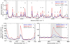 |
Fig. 1 Top panel: example of Jupiter spectral region (zonally averaged) encompassing CH4 lines and the H2O v2 lines at 75∘S (red), 65∘S (blue) and 25∘S (black). The vertical lines display the spectral features of CH4 (black) and NH3 (orange). Bottom left panel: same but for HCN v2 band (zonally averaged) next to C2H2 lines. Bottom right panel: same but for CO2 v2 band. The grey regions mark the positions of the emission lines of each molecule. The spectra at 65∘S is shifted to match the continuum emission of the 75∘S spectrum. The offset values in nWcm−2sr−1/cm−1 are indicated in the legend of each panel. |
3 Modelling
3.1 Radiative transfer code
In the mid-infrared, the contrast of the spectral lines of a given chemical species is mainly due to two factors: (i) the contrast between the temperature at the pressure level that the observations are sensitive to and the temperature of the pressure where the continuum emission is formed; and (ii) the abundance of the molecules that generate the emission line at that pressure level. To retrieve the molecular abundances, we used the same 1D radiative transfer model that was previously used for the retrieval of the temperature and hydrocarbons abundances from the same # 1373 JWST dataset by Rodríguez-Ovalle et al. (2024a). This radiative transfer code accounts for spherical geometry, which is needed to analyse spectra acquired towards the limb of the planet. The model includes 361 vertical layers equally spaced in a logarithmic scale of pressure between 10 and 10−8 bar.
Our model contains spectroscopic information for several molecules present in the atmosphere of Jupiter such as CH4, C2H2, C2H6, NH3, H2O, CO2, and HCN, extracted from the HITRAN database (Gordon et al. 2022). It also includes an opacity source due to the H2-He-CH4 collision-induced absorption spectrum (Borysow et al. 1985, 1988). We coupled our radiative transfer model to a regularized retrieval algorithm that iteratively inverts a posterior vertical profile in order to provide the best estimation of the actual vertical profile. To do so, we compared the observed spectra with the synthetic spectra. The synthetic spectra at the nth iteration was generated using the posterior vertical profile retrieved in that iteration. The iterative changes in the vertical profiles serve to improve the goodness of the spectral fit (χ2/n). This comparison between observed and synthetic spectra continues until a convergence criterion is reached. For each iteration, we used as prior profile the posterior profile resulting from the previous iteration. This iteration continues until the difference of the χ2/n of the current iteration and the previous one is less than 1%. A more in-depth description of the model can be found in Rodríguez-Ovalle et al. (2024a).
3.2 A priori information
To retrieve the CO2, H2O, and HCN abundances, we assumed the temperature and C2H2 and C2H6 abundance 3D-fields retrieved using the same #1373 dataset by Rodríguez-Ovalle et al. (2024a) for the SPR, and the #1246 dataset presented in Harkett et al. (2024) for the GRS. These profiles were derived by fitting the CH4 v4 band centred at 1306 cm−1, the C2H6 v8 band in the 1600–1660 cm−1 range, and the C2H2 v5 band in the 700–666 cm−1 range. For H2O and HCN, as we retrieved only zonal mean abundances, we created zonal-mean profiles for the temperature and abundances, of each tile. For CO2, whose band lies in a different channel than the CH4 v4 band (channel 3 versus channel 2), we re-mapped the retrieved temperature from the channel 2 spaxel size to channel 3 spaxel size (0.277 arcsec for channel 2 and 0.387 arcsec for channel 3). In our dataset, as channel 3 extends to latitudes closer to the equator than channel 2, we assumed a constant temperature profile for the spaxels of channel 3 that were at latitudes not observed in channel 2; that is equatorwards of 53∘S.
The vertical profile of exogenic species has been observed to evolve with time. Following the deposition process around 0.2 mbar in 1994 (Moreno et al. 2003), the species have been migrating to deeper pressure levels, down to ∼3 mbar in 2019 (Benmahi et al. 2020; Cavalié et al. 2023). As our observations, which have a spectral resolution power of R ∼ 3000, do not match in spectral resolution the highly resolved, millimetre heterodyne observations (Lellouch et al. 1997; Moreno et al. 2003; Benmahi et al. 2020; Cavalié et al. 2023), we are not in position to directly infer the vertical distribution of HCN, H2O, and CO2 from our dataset. However, our retrieved column densities may significantly depend on the adopted vertical profiles. Hence, we adopted as a priori the vertical profiles for H2O and HCN measured by Benmahi et al. (2020) using the Odin satellite and Cavalié et al. (2023) using ALMA, respectively. Indeed, we expect minimal evolution in the vertical profiles of these species since the years in which they were lastly observed (respectively 2019 and 2017).
For HCN, Cavalié et al. (2023) inferred three classes of vertical profiles depending on the position on the planet. These vertical profiles were defined by two parameters, the cutoff pressure, and the slope at altitudes below the cutoff pressure. The cutoff pressure separates the higher atmospheric levels (e.g. lower pressures) where the abundance is vertically uniform, from the deeper levels (e.g. higher pressures) where the abundance decreases with pressure. At higher pressures than the cutoff pressure, the slope is expressed as  , where, q is the HCN abundance and p the pressure at the same specific layer.
The three main vertical profiles derived by Cavalié et al. (2023) for the southern hemisphere were: (i) a first profile for latitudes 20∘S–65∘S with a pressure cutoff at 0.3 mbar and a slope of −0.35; (ii) a second profile for polar latitudes between 65∘S and 90∘S, located outside the southern auroral oval, with a cutoff at 0.01 mbar and a slope of −0.8; and (iii) a third profile for latitudes between 65∘S and 90∘S, but located within the southern auroral oval, with a cutoff at ∼0.01 mbar, and a slope of −0.45. We tested these three profiles as a priori profiles and found that a good fit of the HCN line was achieved with all three. More precisely, for the two profiles for polar latitudes, we found that the retrieved column density was very similar in both cases, underlining that the differences in the slope are less important than the pressure of the cutoff. This confirms that, at JWST’s spectral resolution, the HCN line is not sensitive to the detailed vertical profile, but mostly to the cut-off pressure. Consequently, for the retrievals of the HCN abundance profile we decided to use two different profiles (shown in Fig. 2, first row and column), one for latitudes polewards of 65∘S with a cutoff at ∼0.01 mbar and a slope of −0.45, and the other for latitudes equatorwards of 65∘S with a cutoff at ∼0.3 mbar and a slope of −0.35, both of them based on the profiles retrieved by Cavalié et al. (2023).
Finally, the CO2 profile was directly taken from the model used in Moses & Poppe (2017). This model analysed the evolution of exogenic species in the four giant planets. Based on the retrieved abundances for H2O, CO2, and CO after the SL9 impact (Lellouch et al. 2002; Moreno et al. 2003), the model predicted their vertical profiles 23 years after the impact. We used this CO2 profile as prior information for our retrievals. Moreover, we also tested a vertical profile based on the H2O vertical profile from Benmahi et al. (2020) for 2019, divided by a factor of 7, so that the abundances between 10−2 and 1 mbar match the ones of the Moses & Poppe (2017) CO2 predicted profile (see Figure 2). The retrieved column density exhibits minimal alteration when using the H2O-type vertical profile compared with the CO2 vertical profile. For more information on the effects of the different vertical profiles on the retrieved column density of CO2, the reader is directed to Section 4.3.
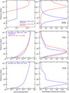 |
Fig. 2 Left column: different vertical profiles used in this work for the three molecules (HCN, CO2, and H2 O) analysed in this work. Right column: contribution functions for the different profiles of each molecule. For CO2 and H2O, the contribution functions correspond to a mean latitude of 60∘S, while for HCN they correspond to a mean latitude of 60∘S for the blue profile, and 75∘S for the red profile. |
3.3 Information content
In Fig. 2, we present the a priori profiles presented in Section 3.2 in the left column, and the corresponding contribution functions for the HCN, CO2, and H2O lines for each vertical profile. These contribution functions demonstrate that the pressure ranges probed by our observations vary as a function of the a priori profile for HCN, due to the change in the cutoff pressure level between the profiles.
The H2O lines lying in the 1600–1660 cm−1 range are sensitive to pressures between 10 and 3 mbar, similar to the pressure levels probed by the CO2 band at 667.5 cm−1. The sounded pressure levels for H2O are similar to that where Benmahi et al. (2020) observed the bulk of the H2O vertical profile in 2019 (∼5 mbar). HCN is the chemical species that probes lower pressures, between 0.5 and 0.01 mbar, depending on the vertical profile used. The CH4 v4 band, used for temperature retrieval, probed the stratosphere within the pressure range of 50–0.01 mbar. This range enables reliable abundance retrievals for HCN, CO2, and H2O, as their contribution functions fall within the probed pressure range of the CH4 v4 band.
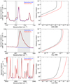 |
Fig. 3 Left: difference in modelled zonally averaged spectra when HCN (55∘S), CO2 (65∘S), and H2O (75∘S) are added (red) and when they are not present (blue) compared with the observations (black). Right: vertical profiles retrieved for each of the molecules. The black profiles corresponds to the a priori profiles used. The red profiles correspond to the retrieved vertical profile for each spectra. |
3.4 Retrieval process
As was mentioned in Section 3.1, the inversion code improves the adjustment to the data by changing a given species vertical profile from its a priori value in the pressure range where the contribution function exhibits significant values. In contrast, at pressure levels where the contribution function is negligible, the inverted vertical profile will remain constrained by the a priori profile.
The range of pressure levels at which the inverted vertical profiles depart from the a priori profiles is determined by the width of the covariance matrix, S. In this study, as the CO2, HCN, and H2O spectral lines are optically thin and lack intrinsic vertical information, we selected a width of ten scale heights for the S matrix. As is explained in Rodríguez-Ovalle et al. (2024a), this choice is essentially equivalent to multiplying the a priori vertical profiles by a constant scaling factor, and assumes the vertical distribution measured in the submillimetre range. Fig. 3 displays an example of the vertical profiles inverted by our model for the three molecules along with the comparison between the forward model and data for the three molecules.
3.5 Fitting the continuum
To ensure a precise continuum fitting around the lines of interest, we made slight adjustments to the temperature profiles presented in Rodríguez-Ovalle et al. (2024a) that were inverted by optimizing the fit over a wider spectral range. Since the continuum is mostly formed at tropospheric levels while the SL9-derived molecules reside in the stratosphere, an adjustment of both the continuum and the abundance of the molecules is possible.
In the vicinity of the HCN and CO2 lines, we started with the temperature profile retrieved using the CH4 v4 band, and the C2H2 abundance profile derived from the whole C2H2 v5 band (Rodríguez-Ovalle et al. 2024a). Then we simultaneously retrieved the HCN and CO2 abundance using their respective emission bands, along with the tropospheric temperature using the emission-induced continuum between the emission lines. The retrieval leaves the temperature profile at pressures smaller than 80 mbar unchanged, keeping the stratospheric temperatures retrieved from the CH4 v4 band unaltered.
In the vicinity of the H2O lines, we also used the temperature profiles from the CH4 v4 band. As for HCN and CO2, a slight change in the temperature profile close to the tropopause level (∼100 mbar) was required to optimally fit the CH4 v2 band (1530–1560 cm−1) on zonal average. Yet, even though small changes were sufficient to fit the 1530–1600 cm−1 region of the continuum well, in the spectral range of 1600–1660 cm−1 the observed spectra still showed lower radiance levels than the synthetic spectra. As it was not possible to obtain a satisfactory fit over the full spectral range by changing the temperature, we also tried to simultaneously modify the tropospheric temperature and the C2H6 vertical profile, but the contribution of this molecule is maximum in the 1510–1540 cm−1 spectral range, and negligible between 1600 and 1660 cm−1. The higher radiance levels modelled compared to observed MRS spectra between 1590 and 1660 cm−1 could thus imply the presence of an additional, unattributed, opacity source near the tropopause, around the 80 mbar pressure level, which diminishes radiance at these specific wavenumbers. We present the differences on the spectral fit when adding an aerosol layer in Fig. 4. The integrated optical thickness required to adjust the spectrum (red curve) to the observed one is ∼3.6 × 10⁻². This value remains constant across latitudes, suggesting a uniform trend. However, we note that the effects of multiple scattering – which are not taken into account in our model – can influence the radiance in this spectral range, as has already been observed on Saturn using MIRI/MRS (Fletcher et al. 2023).
4 Results
4.1 H2O distribution
Figure 5 presents the meridional variation of the H2O column density, for the three different tiles of the #1373 dataset and for the #1246 lower-latitude dataset. Notably, the zonal average column density of stratospheric water in the SPR exhibits a localized enhancement towards the pole in the three tiles, with a mean value of 5.5 ± 0.9 × 10¹⁵ molec cm−2 at 80∘S, a factor 2–3 higher than the column densities found at the edge of the auroral oval at 67∘S. Our retrieved meridional profiles do not show a clear relation with the position of the auroral oval: the tile most covered by the auroral oval has the highest column density southwards of 70∘S, but the least covered tile exhibits an intermediate profile, while the partially covered tile has the lowest column density, most evidently between 70∘S and 75∘S. However, the difference in water column densities between the three tiles remains comparable within the error bars, and does not allow us to establish any strong conclusion. equatorwards of the auroral oval, our analysis also reveals a local maximum of the H2O column density at 60∘S, with a peak value of 2.5 × 10¹⁵ molec cm−2, surrounded by two minima of 1.8 × 10¹⁵ molec cm−2 at 65∘S and 55∘S. This local maximum is not coincident with the position of the SL9 impact (44∘S) or any other recent impacts, such as the 2009 event at 55∘S (Sánchez-Lavega et al. 2010). This peak is present within the three tiles, showing no significant morphological or quantitative differences between the tiles, indicating a longitudinal mixing of the stratospheric H2O outside the south polar region. For the lower-latitudes spectra, only upper limits were obtained due to the lack of detected water lines in this region. The upper limit of ∼1.8 × 10¹⁵ molec cm−2 is consistent with the water being horizontally well mixed at mid-latitudes.
Cavalié et al. (2013) were the first to map H2O in the Jovian upper atmosphere using the 556.936 and 1669.9-GHz lines observed in 2010 with Herschel. With an angular resolution of about a fourth of the Jovian disc, they measured a peak water column density of (4–5) × 1015 molec cm−2 at southern latitudes and a decrease by a factor of up to three towards the northernmost latitudes. Cavalié et al. (2013) underlined that this contrast factor was certainly underestimated due to the spatial convolution by the instrument beam. In this respect, our retrieved maximum column density of 5.5 ± 0.9 × 10¹⁵ molec−2 at 80∘S seems consistent with the Herschel values. Outside the polar regions, our upper limit of ∼1.8 × 10¹⁵ molec cm−2 determined between 17∘S and 26∘S is consistent with the column density of ∼1.5 × 10¹⁵ molec cm−2 value predicted by Benmahi et al. (2020) for the disc-averaged water abundance in 2022.
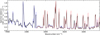 |
Fig. 4 Best synthetic spectrum without aerosols (blue) and with a layer of aerosols that only affect the 1600–1660 cm−1 spectral region (red), compared with the observed spectrum at 73∘S (black). |
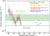 |
Fig. 5 Retrieved meridional trend for H2O for the low latitudes (green), and the three tiles of the SPR: 330∘W in orange, 70∘W in red, and 130∘W in blue. This is compared with the prediction made by Benmahi et al. (2020) for 2022 (disc-averaged), and the measurements of Cavalié et al. (2013) using Herschel/HIFI for the southern polar region. The lowest parallel reached by the southern auroral oval is indicated by a vertical dashed line following Hue et al. (2024). |
4.2 HCN distribution
Fig. 6 presents the retrieved HCN meridional trend for the three tiles of the #1373 ERS dataset and the #1246 GTO dataset. The results are compared with the column density retrieved by Cavalié et al. (2023) using ALMA limb observations. We stress that the HCN and CO column densities presented in Cavalié et al. (2023) were erroneously underestimated by a factor of 10 (Cavalié et al. 2024b). The ALMA measurements presented in Fig. 6 have been corrected by this factor.
Our results show that the HCN column density is meridionally homogeneous from 16∘S to 50∘S, with a value of (3.0 ± 0.6) × 1014 molec−2. Southwards of 50∘S, the column density decreases with latitude by about an order of magnitude at ∼65∘S, and reaches a minimum value of (4.0 ± 0.8 × 10¹² molec cm−2 at 81∘S). In general, our retrieved column densities in 2022 shows strong agreement with the column densities retrieved from ALMA observations in 2017, especially with the profile measured outside the auroral oval.
In contrast to Cavalié et al. (2023) we do not find strong variations in the HCN column density within the auroral oval, as they detected a local maximum in the HCN abundance in the southern auroral region at L = 350∘W. Specifically, this peak eludes the detection in the tiles positioned at 330∘W and 70∘W, corresponding to regions where the auroral oval is visible within the MIRI/MRS FoV. Even more, the meridional profile inferred for the tile most covered by the auroral oval at 70∘W has the lowest column density of the three tiles (yet within error bars). To assess our measurement sensitivity to high altitudes, we conducted a series of tests, using different vertical profiles. The right panel of Figure 7 illustrates two synthetic spectra compared with an observed JWST spectrum at 63∘S. These synthetic spectra were generated by modifying the a priori HCN profile (red and blue lines in the left panel). Notably, changes at pressures lower than the 10-μbar level (red profile) exhibit a negligible impact on the spectra compared to the unaltered scenario (black). This shows that our dataset is only sensitive to pressures higher than 10 μbar, and that the HCN production peak detected by ALMA in the southern aurora can still be compatible with our data. Only ALMA’s spectral resolution power allows for the study of high-altitude chemical processes affecting HCN in the auroral regions of Jupiter.
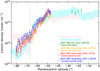 |
Fig. 6 Retrieved meridional trend for HCN column density in this work for the three tiles analysed: 330∘W in orange, 70∘W in red, and 130∘W in blue, compared with previous observations made by Cavalié et al. (2023) with ALMA (pink and cyan). For the latitudes polewards of 65∘S, the HCN vertical profile used is the one with a cutoff at 0.01 mbar. For more equatorward latitudes, we used the profile with a cutoff at 0.5 mbar. The column density was calculated for 10 mbar to 1 μbar. The lowest parallel reached by the southern auroral oval is indicated by a vertical dashed line, following Hue et al. (2024). |
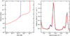 |
Fig. 7 Left: different HCN vertical profiles. Right: resulting synthetic spectrum for these vertical profiles and an observed spectrum at 63∘S (black line). |
4.3 CO2 distribution
The upper panel of Figure 8 presents the retrieved CO2 column density for the three tiles of the #1373 ERS dataset in polar projection. The lower panel of Fig. 8 displays the meridional trends of the retrieved column density zonally averaged over the three tiles of the #1373 ERS dataset, along with the upper limits derived from the #1246 GTO dataset. These results were obtained using the CO2 vertical profile from Moses & Poppe (2017) as the a priori profile. The meridional distributions show, at all longitudes, a rise from an upper limit of 3 × 10¹⁴ molec cm−2 between 17∘S and 26∘S, up to a maximum of (1.9 ± 0.2) × 1015 molec−2 cm−2 at ∼67∘S, followed by a decrease towards higher southern latitudes to reach column densities of (1.1 ± 0.3) × 1015 molec cm−2 at ∼78∘S. From mid-latitudes to 67∘S, our derived column densities nicely agree with (although they are slightly lower than) the ones derived by Lellouch et al. (2006) using Cassini/CIRS (gray values in the lower panel of Fig. 8). However, southwards of 67∘S, Lellouch et al. (2006) found the CO2 column density reaching a plateau at a value of ∼2.3 × 10¹⁵ molec cm−2, while we find a steady polewards decrease at all longitudes. The discrepancy with the meridional distribution observed in Lellouch et al. (2006) could conceivably be attributed to an imprecise assumption about stratospheric temperatures in their study. The latitudinal selection of spectra for CO2 in Lellouch et al. (2006) did not distinguish between auroral and non-auroral longitudes. As was shown in Figure 1 of their work, they assumed a maximum temperature of 165 K at 0.5 mbar for latitudes southwards of 70∘S, with a temperature difference of approximately 5 K compared to 60∘S. However, recent studies have indicated that the temperature contrast is likely larger within the aurora, with temperatures reaching up to 180 K at 0.5 mbar for latitudes southwards of 70∘S (Sinclair et al. 2023; Rodríguez-Ovalle et al. 2024a). In an extreme situation, assuming a 180 K temperature at 0.5 mbar instead of 165 K leads to a change in the Planck function at the CO2 peak frequency by a factor of 1.63, implying that the CO2 amounts polewards of 70∘S from Lellouch et al. (2006) could have been overestimated by the same factor (given that the CO2 emission is mostly optically thin). Although it is difficult to track down this issue more precisely, it seems plausible that at least part of the difference in the CO2 latitudinal profile between Lellouch et al. (2006) and the present study may be ascribed to temperature effects.
In terms of longitudinal distribution, at first glance, the CO2 distribution seems quite homogeneous (upper panel of Fig. 8). However, the meridional profiles show subtle differences at higher latitudes, with the mean CO2 column density being higher by a factor 1.5 in the tile centred at 130∘W compared to the two other tiles, for latitudes polewards 74∘S.
The CO2 results using the H2O-type vertical profile as a priori profile are shown in Appendix A, and are very similar to the ones shown in this section.
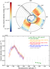 |
Fig. 8 Top: polar projection of the column density of CO2 in the south polar region. The black lines mark the statistical position of the UV auroral oval (Bonfond et al. 2017). Bottom: retrieved meridional trend for CO2 in this work (red), compared with previous observations made by Lellouch et al. (2006) with Cassini/CIRS. |
5 Discussion
The chemical products of the SL9 collision reveal a diversified and puzzling chemical evolution. In the south polar region, the three species exhibit different behaviours: the HCN abundance decreases poleward; the CO2 abundance increases towards the south pole until it reaches a maximum at 67∘S (i.e., near the statistical position of the auroral main oval) and then starts a decrease towards the south pole; and te H2O abundance increases towards the south until it reaches a local maximum at ∼60∘S, then it decreases until it reaches a local minimum at 65∘S and finally increases towards the south pole. Such different meridional profiles, with maxima and minima located at different latitudes, reveal several different chemical processes at play in the Jovian polar atmosphere.
5.1 HCN
In our analysis, we observe that HCN follows a similar latitudinal distribution as the one observed in 2017 using ALMA (Cavalié et al. 2023). Our JWST meridional profile and the ALMA meridional profile match in terms of absolute HCN column density and in the overall magnitude of the decrease occurring southwards of 55∘S.
The fact that the two measurements match so closely, separated by five years, may even appear surprising. According to Cavalié et al. (2024b), the total HCN column density was depleted by a factor of 12.0 ± 3.5 between 2000 and 2017. If we extrapolate this trend to 2022, a depletion of a factor of 2.1 ± 0.2 should be expected in our 2022 observations with respect to the 2017 ALMA observations. However, the combined error bars of the ALMA and JWST also amount to a factor of ∼2 or more. We thus think that our uncertainties are still too large to monitor the HCN destruction between 2017 and 2022, but we cannot rule out the possibility that the HCN column density remained unchanged during this time interval.
The absence of a polar depletion in the CO column density measured by Cavalié et al. (2023) suggested that polar vortices might not fully account for the meridional trend in the HCN distribution, as was proposed by Lellouch et al. (2006). Cavalié et al. (2023) proposed an alternative explanation, invoking heterogeneous chemistry triggered by the presence of stratospheric aerosols. Their proposal was based on ALMA observations, which constrained HCN polar depletion to pressures greater than 0.1 mbar – a pressure range where aerosols settle. In contrast, Cavalié et al. (2023) did not favour ionic chemistry for HCN, as pressures this high are inaccessible to precipitating electrons. While our MIRI spectra do not allow us to vertically profile HCN, the JWST #1373 dataset still brings further elements supporting this proposal. As is detailed in Rodríguez-Ovalle et al. (2024b), in the south polar region JWST identified stratospheric polar aerosols in the near- and mid-infrared, and detected C6H6, thought to be a precursor of polar aerosols (Wong et al. 2003). In NIRCam images obtained at 3.23 μm (in Rodríguez-Ovalle et al. (2024b), Fig. 3), the solar reflection from stratospheric polar aerosols fades into the mid-latitude albedo level at latitudes between 60∘S and 50∘S. The inferred benzene column density also monotonously decreases from 80∘S to ∼55∘S, where it reaches a latitudinally homogeneous distribution (see Rodríguez-Ovalle et al. (2024b), their Fig. 7). In the mid-infrared, Rodríguez-Ovalle et al. (2024b) could not assert that the transition between the polar region and the mid-latitudes takes place at 50–60∘S, as the aerosol spectral features identified at 700, 750 and 1450 cm−1 became undetectable equatorwards of 60∘S and 70∘S, respectively. However, the opacity of these three features clearly decreases equatorwards from a maximum located at 80∘S. The limit at ∼55∘S hence appears as a transition between the south polar region and the rest of the planet.
As an alternative explanation, Moses et al. (2023) studied the ion-neutral chemistry induced by the ring material falling into Saturn’s upper atmosphere and proposed that ion-neutral reactions could act as a sink of HCN by forming heavier molecules, such as HC3N or CH3CN. These species could then condense and effectively remove nitrogen from detection. While our dataset does not allow us to rule out this hypothesis, it should be further tested by attempting to measure the abundances or upper limits of these two species, which have not yet been detected in Jupiter’s atmosphere.
We have further used our retrieved HCN meridional profile to estimate the loss rate of HCN in the polar region and compare it with the global depletion rate measured by Cavalié et al. (2023). For this, we have used the continuity equation integrated vertically,
 (1)
(1)
where θ is the latitude, r the planetary radius, Kyy the horizontal eddy diffusion coefficient, N the HCN column density, and L the vertically integrated loss rate per surface area. This loss rate was then integrated over the surface of the polar regions, between θ1 = 80∘S and θ2 = 50∘S:
 (2)
(2)
In the derivation of Eq. (1), we have made several hypotheses. First, we have assumed steady state by neglecting  , which is equivalent to assuming that the HCN abundance latitudinal profile in the polar region is in a steady state due to the balance between local chemical loss and eddy transport. In this respect, our assumption gives an upper bound of the actual chemical loss rate, this upper bound being limited by the diffusion efficiency from mid-latitudes towards the pole. Secondly, we have assumed that the eddy mixing coefficient is vertically and latitudinally uniform. Such an assumption is questionable, since the existence of a south polar vortex linked to the auroral oval was evidenced at 0.1 mbar from the ALMA wind measurements obtained by Cavalié et al. (2021). Such a vortex should inhibit or reduce material transport between regions inside and outside the vortex. Lellouch et al. (2006) also proposed a Kyy meridional profile with lower values, by at least one order of magnitude, in the SPR than at mid-latitudes to reproduce their observed HCN profile. We discuss these hypotheses below.
The inferred loss rate from Eqs. (1) and (2) is directly proportional to the adopted value for eddy mixing coefficient. Moreno et al. (2003) and Lellouch et al. (2006) have inferred possible values from fitting the equatorwards spread of CO and HCN, assuming negligible chemical loss. They proposed, respectively, Kyy = 2.5 × 1011 cm2 s−1 and Kyy = 2.0 × 1011 cm2 s−1. Assuming a mean of their values yields a total loss rate of (1.8 ± 0.2) × 1027 s−1. This rate should be compared with the decrease in the planetary integrated mass of HCN measured by Cavalié et al. (2023). In 2017, they measured a total mass of (5.0 ± 0.1) × 1012 g, and deduced a loss factor of 12.0 ± 3.5 with respect to the value measured in 2000 from the Cassini/CIRS data, which corresponds to a loss rate of (2.4 ± 0.7) × 1027 s−1 over the period. These two figures agree remarkably closely, suggesting that heterogeneous chemistry in the polar regions is the dominant HCN destruction mechanism in Jupiter’s stratosphere. However, this agreement should be interpreted with caution due to the hypotheses we have made on the eddy mixing coefficient absolute value and latitudinal profile.
A larger eddy mixing coefficient – increasing polewards would increase the HCN flux from mid-latitudes towards the SPR. A larger flux such as this would need to be balanced either by a higher loss rate in the SPR, or by a build-up with time in the HCN abundance over the SPR. The latter seems to be ruled out as the contrast between the mid-latitude and south polar abundances has increased from a factor of ∼10 in 2000 (Lellouch et al. 2006) to a factor of ∼100 in 2017–2022 as revealed by Cavalié et al. (2023) and our study. The former solution, a larger loss rate in the SPR, is ultimately limited by the fact that it cannot be larger than the planetary integrated loss rate measured by Cavalié et al. (2023). So the actual eddy mixing coefficient can hardly be larger than twice our adopted value of Kyy = 2.25 × 1011 cm2 s−1.
Alternatively, the eddy mixing coefficient could be lower than Kyy = 2.25 × 1011 cm2 s−1, or decreasing sharply polewards as was hypothesized by Lellouch et al. (2006). The resulting lower transport would need to be balanced by a smaller loss rate in the SPR, or by a decrease with time in the HCN abundance. The HCN abundance in the SPR has indeed decreased between 2000 and 2017–2022, but not more drastically than at mid-latitudes. Therefore, a lower eddy mixing coefficient would rather mean that the dominant HCN destruction mechanism is not heterogeneous chemistry in the SPR but HCN photolysis at mid-latitudes. To investigate this hypothesis further, we calculated the photochemical lifetime of HCN with a simple atmospheric model. The HCN UV cross-sections were taken from Nuth & Glicker (1982) and Lee (1980), and the CH4 cross-sections from Backx et al. (1975), Lee & Chiang (1983), and Mount et al. (1977). Using the solar reference spectrum from Thuillier et al. (2004), we calculated a HCN photolysis rate of 1.26 × 10⁻⁶ s−1 at the top of the atmosphere, in good agreement with the calculations of Moses (1996). At 1 mbar, we further estimated the HCN photolysis timescale to be 27 terrestrial years, and 37 years at 3 mbar, where most of the HCN now resides. These estimates must be considered as lower limits of the HCN photolysis timescale, as our model does not take into account either Rayleigh scattering or additional photolysis shielding by C2H6 and C2H2. Still, these estimates are much longer than the characteristic e-folding time of seven years inferred by Cavalié et al. (2023).
We thus propose a self-consistent picture composed of two elements: the main current HCN chemical loss is heterogeneous chemistry on polar aerosols, and there is a lack of a dynamical barrier between the south polar region and mid-latitudes. This lack of a dynamical barrier is further supported by several measurements showing an efficient transport mechanism between polar and non-polar regions. First, the SL9-derived CO now exhibits a quasi-pole-to-pole homogeneous distribution at 3 mbar, as was retrieved by Cavalié et al. (2023) using ALMA. Secondly, the maps of the aurorally produced aerosols and benzene (Rodríguez-Ovalle et al. 2024b; Sinclair et al. 2020) do not exhibit any sharp abundance gradient that would reveal a transport barrier. In contrast, they exhibit instead a smooth, constant, gradient from their production regions towards mid-latitudes.
We caution the reader that this picture needs to be validated by more detailed models that should include other parameters, such as vertical transport, as aerosols do sediment, and their vertical profile is far from homogeneous. The HCN loss rate must hence be higher at higher pressure, and the HCN vertical transport time could hence limit the chemical loss in the polar regions. In addition, Cavalié et al. (2023) propose that aurorally driven HCN production takes place in the 1–10 μbar pressure range, in the south polar region, a finding that further complicates the picture. Our JWST observations, taken at a medium spectral resolution are not sensitive to such low pressures and we cannot confirm the HCN increase reported within the auroral oval by Cavalié et al. (2023). This could suggest a potential altitude threshold for auroral HCN production above the 0.01-mbar pressure level. However, we cannot rule out that the differences between our investigation and the results of Cavalié et al. (2023) could be due to time-variable phenomena, which have been extensively documented in polar regions (Sinclair et al. 2023; Rodríguez-Ovalle et al. 2024a). In any case, our data are insufficient to fully constrain a 2D transport-chemistry model.
5.2 Oxygenated species
In this study, we have analysed the H2O and CO2 spatial distributions at southern polar latitudes. Our measurements represent a significant advancement, as they provide the first CO2 meridional distribution since the Cassini-CIRS observations in 2000 (Lellouch et al. 2006). Moreover, the improved spatial resolution provided by MIRI has allowed us to extend our analysis across three different longitude ranges. For H2O, this study presents the first high-resolution measurement at polar latitudes, surpassing previous observations made using Herschel observations (Cavalié et al. 2013), which were limited to latitudes between 60∘N and 60∘S due to lower resolution capabilities.
In general, retrieved column densities for CO2 and H2O are approximately an order of magnitude lower than the mean CO column density retrieved by Cavalié et al. (2023) (∼2 × 10¹⁶ molec cm−2), showing that CO remains the dominant stratospheric oxygen-bearing species. For CO2 (see Fig. 8), the retrieved column densities between 50∘S and 67∘S closely match the ones inferred in 2000 by Lellouch et al. (2006). Additionally, our upper limit of 3 × 10¹⁴ molec cm−2 at low latitudes (17∘S–26∘S) is consistent with their reported value of (5 ± 2) × 1014 molec cm−2 at mid-latitudes. For H2O (see Fig. 5), the column densities retrieved from MIRI/JWST in the SPR are on average slightly lower than the Herschel measurements (3.2 × 10¹⁵ molec cm−2) for the same region (Cavalié et al. 2013), but are larger than the disc-averaged predictions of 1.5 × 10¹⁵ molec cm−2 by Benmahi et al. (2020). At mid-latitudes, our upper limit of 1.7 × 10¹⁵ molec cm−2 is about half of the south polar values provided by Herschel, but remains consistent with the disc-averaged predictions for 2022. This upper limit is also marginally smaller than the disc-averaged value of (2.0 ± 0.5) × 1015 molec cm−2 measured in 1997 by Lellouch et al. (2002).
While our analysis reveals a CO2 column density similar to the one observed in 2000 at non-auroral regions (Lellouch et al. 2006), a remarkable difference emerges within the southern auroral region, as is shown in Figure 8. Specifically, our findings show that the CO2 column density decreases southwards, from a maximum of (2.0 ± 0.2) × 1015 molec cm−2 at 67∘S to (1.2 ± 0.2) × 1015 molec cm−2 at 77∘S. In addition, at auroral latitudes, we observe a higher CO2 column density in the 135∘W tile, where the auroral oval is absent from the MIRI/MRS FoV, compared to the 335∘W and 70∘W tiles, where the auroral oval is fully or partially present.
This depletion of CO2 within the auroral region becomes even more striking when juxtaposed with the observed increase in the H2O column density within the same region. The H2O column density rises from (2.0 ± 0.2) × 1015 molec cm−2 at 67∘S to (5.5 ± 0.5) × 1015 molec cm−2 at 80∘S. This elevated H2O column density in auroral region is consistent with Herschel/HIFI observations, which indicated slightly higher water abundances near the southern pole (Cavalié et al. 2013). At lower latitudes, between 60∘S and 67∘S, the southwards increase in CO2 also coincides with a decrease in H2O. Even though this suggests an intricate evolution of both species, not all of our measurements follow this trend. For instance, between 55∘S and 60∘S, both species increase towards the south. In addition, within the auroral region, the tile fully covered by the auroral oval (70∘W) exhibits the highest H2O abundance, while the partially covered tile (330∘W) has the lowest abundance, and the tile located fully outside the oval (135∘) exhibits intermediate values.
Figure 9 shows the mean meridional trend of the two oxygen-bearing species analysed in this work, CO2 and H2O (upper row) for the three MIRI/MRS tiles. This figure also displays the total number of oxygen atoms per cm−2 in these two species (lower row), calculated by summing their column densities, each multiplied by the number of oxygen atoms in the respective molecule. This figure highlights the anti-correlation between CO2 and H2O in the latitude range 60∘S–80∘S. An analysis of the Spearman’s ρ coefficient for the distributions of CO2 and H2O gives values of ∼−0.8 and p values lower than 0.005, which indicates a very strong anti-correlation between the two molecules (Corder & Foreman 2014). For the total number of oxygen atoms, we observe an approximately constant trend, with a similar mean value across the three tiles (∼6 × 10¹⁵ atoms cm−2). Combined with the latitudinally well-mixed profile of CO reported by Cavalié et al. (2023), this constant trend indicates that the oxygen introduced by SL9 impacts are primarily carried by CO, followed by CO2 and H2O, and that other possible oxygenated species (CH3OH, H2CO …) should have weak abundances.
Using a simple photochemical model, Lellouch et al. (2002) predicted the oxygen partitioning between CO, H2O, and CO2 as a function of time, as is shown in their Figure 12. While the CO volume remained constant in their model, CO2 was predicted to increase for up to 55 years following the SL9 impact, and H2O would undergo a gradual depletion starting roughly six years after the impact. This predicted evolution of CO seems in agreement with recent observations obtained in 2017 (Cavalié et al. 2023), with column densities comparable with that retrieved in 1995–1998 by Moreno et al. (2003). However, by the time of our observations, Lellouch et al. (2002) predicted a nearly twofold increase in global CO2 column density compared to values retrieved in 2000 (Lellouch et al. 2006). Although our dataset cannot provide a planetary-integrated CO2 mass estimate, our results do not seem to support the global CO2 increase predicted by Lellouch et al. (2002). Firstly, our upper limit derived for the low latitudes between 17∘S and 26∘S is incompatible with a doubling of local column density since 2000 (Lellouch et al. 2006). Secondly, while our measurements between 50∘S and 67∘S are slightly lower than but still consistent with the ones from 2000, CO2 at more southern latitudes appears to be depleted compared to the time of the Cassini flyby. Similarly, we cannot assess the need for an additional H2O loss mechanism beyond photochemistry, as is proposed by the model introduced in the PhD manuscript of Benmahi (2022). In contrast, our measurements provide new insights into chemical evolution at small spatial scale, revealing previously undetected localized trends. To explain these trends, we consider three possible mechanisms: precipitation of oxygen ions, auroral chemistry, or heterogeneous chemistry; however, none is definitively favoured by our observations.
First, following Lellouch et al. (2006), oxygen ions precipitating from Io’s plasma torus could affect the oxygen budget in the SPR, primarily contributing to the production of water molecules. Similar conclusions were reached in studies of ionized oxygen influx into Saturn’s upper atmosphere by Moore et al. (2015) and Moses et al. (2023). However, estimating the external contribution to Jupiter’s total oxygen budget remains challenging, as the only estimates of this external flux covers a broad range: 1026−1027 s−1 (Gehrels & Stone 1983). Over 30 years, such an influx could have delivered between 1035 and 1036 oxygen atoms to the whole planet. The upper end of this range is comparable to the total number of oxygen atoms we observed in H2O and CO2 between 60∘S and 80∘S. However, this amount would still be buffered by the tenfold larger reservoir of oxygen atoms in CO. Given the current uncertainties in these estimates (Fig. 9), it remains difficult to assess the effect of these external contributions.
Even if the CO column density is ∼10 times larger than the ones of CO2 and H2O, and hence can act as a buffer for oxygen, the constant trend in the total number of oxygen atoms carried by CO2 and H2O supports the scenario of oxygen exchange between CO2 and H2O. Regarding the chemical pathways involved in this oxygen exchange, ion-neutral chemistry in the auroral regions seems a likely culprit, our second possible mechanism. Unfortunately, the influence of charged particle precipitation in the atmospheres of giant planets remains relatively understudied (see the review of Hue et al. 2024). Benmahi et al. (2020) analysed 18 years of the 557-GHz H2O line evolution using Odin satellite, revealing a decay in both the global water column density and the water residing altitude (5-mbar pressure level in 2020). To explain this decay, Benmahi (2022) proposes a preliminary chemical scheme to account for this depletion of H2O and CO2 production:
 (3)
(3)
 (4)
(4)
 (5)
(5)
 (6)
(6)
On the other hand, Dobrijevic et al. (2020) provide valuable insights into auroral chemistry, particularly for Neptune. Their detailed model simulations suggest an opposite scenario to the one presented in Benmahi (2022), whereby charged particle precipitation could indeed influence H2O and CO2 concentrations, leading to increased H2O levels and concurrent CO2 destruction, while leaving CO relatively unaffected. These results offer a compelling parallel to the observations in Jupiter’s atmosphere southwards of 67∘S. However, it is important to acknowledge the limitations and uncertainties in their model. Dobrijevic et al. (2020) found the highest CO2 depletion to occur at the microbar level, but noted that this prediction may depend on the eddy diffusion coefficient. Moreover, while their findings constitute an interesting mechanism for Jupiter, it is crucial to recognize that the specific parameters governing auroral chemistry may differ between Jupiter and Neptune.
The contradictory processes proposed by Benmahi et al. (2020) and Dobrijevic et al. (2020) could both be active in Jupiter’s south polar region, with their relative magnitudes varying with latitude. This would imply that environmental parameters may favour one process over the other depending on latitude. One key parameter that could impact the efficiency of each process is the energy of precipitating electrons, which varies across the auroral region. On the auroral oval, the energy deposited can reach up to 400 keV (according to Benmahi et al. (2024), their Figures 7 and 9), while in the inner part of the auroral oval, the electron energy is lower (under 100 keV). Another possible parameter is the eddy diffusion coefficient. Auroral precipitation can potentially shift the homopause altitude (Sinclair et al. 2020; Rodríguez-Ovalle et al. 2024a), resulting in a higher homopause altitude within the auroral oval than in surrounding areas. This is likely due to a larger eddy diffusion coefficient Kzz within the auroral oval than in its vicinity.
Unfortunately, the sensitivity of the processes proposed by Benmahi et al. (2020) and Dobrijevic et al. (2020) to these two environmental parameters remains uncertain. Given these uncertainties, it is challenging to establish a definitive understanding of the ion-neutral chemistry occurring in Jupiter’s south polar region and its impact on the local and global abundances of CO2 and H2O.
We must also emphasize that invoking ion-neutral chemistry to explain the meridional profiles of CO2 and H2O presents a significant difficulty, both in terms of the assumed vertical profiles for these two species, and our retrieved CO2 longitudinal distribution. As was noted earlier for HCN, ion-neutral chemistry can only produce and destroy molecules in the upper stratosphere (p < 10 μbar), several scale heights above the pressure levels (p ∼ 3 mbar) where the bulk of the CO2 and H2O is assumed to reside. The typical diffusion timescales between these two pressure levels appear too long for auroral-induced chemistry to be solely responsible for the observed behaviour of CO2 and H2O. This discrepancy could be mitigated if the vertical distributions of CO2 and H2O differ from our assumptions and are more concentrated at higher altitudes. We cannot rule out this possibility, as our dataset does not allow us to retrieve the species’ vertical profiles, and because submillimetre heterodyne observations of H2O lack the angular resolution to infer the water vertical profile within the SPR (Benmahi et al. 2020; Cavalié et al. 2013). However, such an alternative scenario conflicts with the current model that H2O and CO2 are daughter molecules of CO, which has been firmly measured to reside at around 3 mbar (Cavalié et al. 2023). It also conflicts with the longitudinal distribution we measured for CO2 (Fig. 8). Unlike the findings of Rodríguez-Ovalle et al. (2024a) for C2H2, the CO2 abundance does not appear to be enhanced or reduced within the auroral oval, challenging its link with auroral-induced chemistry. Instead, the deep, longitudinally symmetric alteration of the CO2 abundance in auroral regions more closely resembles the signature of a third possible mechanism, heterogeneous chemistry, similar to what is observed for HCN. However, we are not aware of any existing proposed chemical mechanisms or experimental study that could account for this process.
In front of these contradictions, further insights could be obtained by studying the northern polar region (NPR). In the NPR, the auroral oval has a different geometry than in the SPR, being more offset from the pole, larger in area, and with a different energy precipitation (Benmahi et al. 2024). This different geometry may help to disentangle the two proposed chemical schemes and test their sensitivity to environmental parameters. In addition, we note that Cavalié et al. (2013) found an asymmetry in the meridional distribution of the H2O column density, with a maximum at southern latitudes and a minimum in the northern hemisphere. It could be due to a more efficient destruction of water in the NPR, but we cannot rule out that water vapor was not yet latitudinally well mixed at the time of their observations in July 2010.
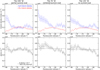 |
Fig. 9 Top: meridional trend of H2O and CO2 extracted from this work. Bottom: quantity of oxygen atoms from H2O and CO2 as a function of latitude. The dashed lines show the mean value of the oxygen atoms in each of the tiles analysed. This trend appears to be constant, suggesting an oxygen exchange between CO2 and H2O in the auroral region. |
6 Conclusion
In this work, we have analysed the abundances of three exogenous species on Jupiter, H2O, CO2, and HCN, using JWST MIRI/MRS observations. We have used the ERS #1373 dataset, which targeted the south polar region at latitudes polewards of 47∘S for HCN and CO2 (channel 3-MEDIUM), and 53∘S for H2O (channel 1-MEDIUM). In addition, we have used the GTO #1246 dataset, which focused on the GRS (22∘S).
Our retrieval of the HCN column density yields a similar trend to the one observed in 2017 by Cavalié et al. (2023), although we could not identify a local maximum in its abundance within the southern auroral oval as was identified in their study. Our analysis suggests that the HCN ν2 band analysed lacks sensitivity to pressures below 0.01 mbar, where aurorally driven HCN production may primarily occur. Globally, our retrieved HCN meridional trend shows a strong decrease towards the south pole. From the observed poleward decrease, we infer that the local destruction mechanism, most likely heterogeneous chemistry on polar aerosols, should be the dominant mechanism responsible for the planetary-average decrease in the HCN abundance.
Regarding CO2 and H2O, our findings reveal an interesting contrast: inside the southern auroral region, CO2 presents a local depletion and H2O a local increase, while at the mid-latitude edge of the auroral region CO2 reaches a local maximum and H2O drops to a local minimum. This opposite behaviour between CO2 and H2O abundances suggests that oxygen exchange between the two species may be a key driver of oxygen chemistry in Jupiter’s south polar region. However, the driving mechanisms remain unclear. If ion-neutral chemical schemes proposed by Benmahi (2022) and Dobrijevic et al. (2020) could theoretically produce either CO2 or H2O at the expense of the other, it is still unknown if these schemes actually take place or if other mechanisms such as oxygen precipitation from the plasma torus or heterogeneous chemistry can also play a role in the oxygen chemistry.
In summary, this study underscores the complex nature of chemistry in Jupiter’s polar region, highlighting the necessity for comprehensive chemical models that incorporate ion-related pathways including oxygen-bearing molecules. The sensitivity of these chemical pathways to various environmental parameters should also be deeply investigated. In parallel, a better characterization of these environmental parameters is needed. The remarkable capabilities of JWST may play a key role in this endeavour. In particular, additional JWST observations at low-to-mid-latitudes and across the NPR of Jupiter are needed to disentangle the proposed chemical scenarios. The upcoming JUICE mission will also constitute a significant leap forwards. Indeed, the Moons and Jupiter Imaging Spectrometer (MAJIS) will document the auroral precipitation effects in the near-infrared by mapping  and CH4 emissions, and the Sub-millimeter Wave Instrument (SWI) will provide three-dimensional scans of the temperature, and CO, HCN, and H2O abundances, revealing the vertical chemical structure that we are currently lacking.
Data availability
Level-3 calibrated Jupiter MIRI/MRS data from the standard pipeline are publicly available through the MAST archive at https://mast.stsci.edu/portal/Mashup/Clients/Mast/Portal.html (MISSION: JWST, PROPOSAL-ID: 1373).
The radiative transfer and retrieval code utilized in this work, as well as in previous studies (Fouchet et al. 2016; Guerlet et al. 2009), is available for download at Rodriguez-Ovalle (2024).
The JWST calibration pipeline used in this study (version 1.11.3) can be accessed via Bushouse et al. (2022). The data products generated in this study are available at Rodríguez-Ovalle & Fouchet (2025).
Acknowledgements
This work is based on observations obtained with the NASA/ESA/CSA James Webb Space Telescope. The data were obtained from the Mikulski Archive for Space Telescopes at the Space Telescope Science Institute, which is operated by the Association of Universities for Research in Astronomy, Inc., under NASA contract NAS 5-03127 for JWST. These observations are associated with program #1373 (Observations 2, 4 and 26), which is led by co-PIs Imke de Pater and Thierry Fouchet. GTO #1246 program was led by PI Leigh N. Fletcher. Data from JWST program 1246 was used for wavelength calibration. PRO was supported by an Université Paris-Cité contract. TF & EL acknowledge support from the ANR PRESSE ANR-21-CE49-0019. TC acknowledges funding from CNES and from the Programme National de Planétologie. VH acknowledges support from the French government under the France 2030 investment plan, as part of the Initiative d’Excellence d’Aix-Marseille Université – A*MIDEX AMX-22-CPJ-04. IdP is in part supported by the Space Telescope Science Institute grant JWST-ERS-01373. LNF was supported by STFC Consolidated Grant reference ST/W00089X/1. JH was supported by an STFC studentship. We wish to express our gratitude to Julie Moses for providing the vertical profiles of H2O and CO2 (taken from Moses & Poppe 2017) that were used in this work. For the purpose of open access, the authors have applied a Creative Commons Attribution (CC BY) license to the Author Accepted Manuscript version arising from this submission.
Appendix A CO2 abundances using the H2O profile
Fig. A.1 presents the abundances and column density of CO2 when using the H2O profile retrieved in Cavalié et al. (2019) for 2019, but rescaling it to match the abundances of the CO2 profile obtained in Moses & Poppe (2017) in the 5 = 0.5 mbar pressure range.
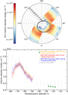 |
Fig. A.1 Same figure as in Fig. 8 but using the H2O profile rescaled to match the CO2 abundances in the stratosphere. |
References
- Backx, C., Wight, G. R., Tol, R. R., & Van der Wiel, M. J. 1975, J. Phys. B At. Mol. Phys., 8, 3007 [Google Scholar]
- Bézard, B., Griffith, C. A., Kelly, D. M., et al. 1997, Icarus, 125, 94 [Google Scholar]
- Bézard, B., Lellouch, E., Strobel, D., Maillard, J.-P., & Drossart, P. 2002, Icarus, 159, 95 [CrossRef] [Google Scholar]
- Benmahi, B. 2022, Étude de la dynamique et de la composition des atmosphères des planètes géantes: préparation de la mission JUICE, PhD thesis, Université de Bordeaux, France [Google Scholar]
- Benmahi, B., Cavalié, T., Dobrijevic, M., et al. 2020, A&A, 641, A [Google Scholar]
- Benmahi, B., Bonfond, B., Benne, B., et al. 2024, A&A, 685, A [Google Scholar]
- Bjoraker, G. L., Stolovy, S. R., Herter, T. L., Gull, G. E., & Pirger, B. E. 1996, Icarus, 121, 411 [Google Scholar]
- Bonfond, B., Gladstone, G. R., Grodent, D., et al. 2017, Geophys. Res. Lett., 44, 4463 [NASA ADS] [CrossRef] [Google Scholar]
- Borysow, J., Trafton, L., Frommhold, L., & Birnbaum, G. 1985, Astrophys. J., 296, 644 [Google Scholar]
- Borysow, J., Frommhold, L., & Birnbaum, G. 1988, Astrophys. J., 326, 509 [Google Scholar]
- Bushouse, H., Eisenhamer, J., Dencheva, N., et al. 2022, https://doi.org/10.5281/zenodo.7038885 [Google Scholar]
- Cavalié, T., Feuchtgruber, H., Lellouch, E., et al. 2013, A&A, 553, A [Google Scholar]
- Cavalié, T., Hue, V., Hartogh, P., et al. 2019, A&A, 630, A [Google Scholar]
- Cavalié, T., Benmahi, B., Hue, V., et al. 2021, A&A, 647, L [Google Scholar]
- Cavalié, T., Rezac, L., Moreno, R., et al. 2023, Nat. Astron., 7, 1048 [CrossRef] [Google Scholar]
- Cavalié, T., Lunine, J., Mousis, O., & Hueso, R. 2024a, Space Sci. Rev., 220, 8 [Google Scholar]
- Cavalié, T., Rezac, L., Moreno, R., et al. 2024b, Nat. Astron., 8, 1206 [Google Scholar]
- Connerney, J. E. P. 1986, Geophys. Res. Lett., 13, 773 [Google Scholar]
- Corder, G. W., & Foreman, D. I. 2014, Nonparametric Statistics: A Step-by-Step Approach, 2nd ed. (Hoboken, N., USA: Wiley) [Google Scholar]
- Dobrijevic, M., Loison, J. C., Hue, V., Cavalié, T., & Hickson, K. M. 2020, Icarus, 335, 113375 [NASA ADS] [CrossRef] [Google Scholar]
- Feuchtgruber, H., Lellouch, E., de Graauw, T., et al. 1997, Nature, 389, 159 [Google Scholar]
- Fletcher, L. N., King, O. R. T., Harkett, J., et al. 2023, J. Geophys. Res. Planets, 128, e2023JE007924 [NASA ADS] [CrossRef] [Google Scholar]
- Fouchet, T., Greathouse, T. K., Spiga, A., et al. 2016, Icarus, 277, 196 [NASA ADS] [CrossRef] [Google Scholar]
- Gehrels, N., & Stone, E. C. 1983, J. Geophys. Res., 88, 5537 [Google Scholar]
- Gordon, I. E., Rothman, L. S., Hargreaves, R. J., et al. 2022, J. Quant. Spectrosc. Radiat. Transfer, 277, 107949 [NASA ADS] [CrossRef] [Google Scholar]
- Griffith, C. A., Bézard, B., Greathouse, T., et al. 2004, Icarus, 170, 58 [Google Scholar]
- Guerlet, S., Fouchet, T., Bézard, B., Simon-Miller, A. A., & Michael Flasar, F. 2009, Icarus, 203, 214 [NASA ADS] [CrossRef] [Google Scholar]
- Harkett, J., Fletcher, L. N., King, O. R. T., et al. 2024, J. Geophys. Res. Planets, 129, e2024JE008415 [Google Scholar]
- Hue, V., Cavalié, T., Sinclair, J. A., et al. 2024, Space Sci. Rev., 220, 1 [Google Scholar]
- King, O. R. T., Fletcher, L. N., Harkett, J., Roman, M. T., & Melin, H. 2023, Res. Notes AAS, 7, 223 [Google Scholar]
- Landgraf, M., Liou, J.-C., Zook, H. A., & Grün, E. 2002, Astron. J., 123, 2857 [Google Scholar]
- Lee, L. C. 1980, J. Chem. Phys., 72, 6414 [Google Scholar]
- Lee, L. C., & Chiang, C. C. 1983, J. Chem. Phys., 78, 688 [Google Scholar]
- Lellouch, E., Paubert, G., Moreno, R., et al. 1995, Nature, 373, 592 [Google Scholar]
- Lellouch, E., Bézard, B., Moreno, R., et al. 1997, Planet. Space Sci., 45, 1203 [NASA ADS] [CrossRef] [Google Scholar]
- Lellouch, E., Bézard, B., Moses, J. I., et al. 2002, Icarus, 159, 112 [Google Scholar]
- Lellouch, E., Moreno, R., & Paubert, G. 2005, A&A, 430, L [Google Scholar]
- Lellouch, E., Bézard, B., Strobel, D. F., et al. 2006, Icarus, 184, 478 [Google Scholar]
- Li, C., Ingersoll, A., Bolton, S., et al. 2020, Nat. Astron., 4, 609 [Google Scholar]
- Marten, A., Gautier, D., Griffin, M. J., et al. 1995, Geophys. Res. Lett., 22, 1589 [CrossRef] [Google Scholar]
- Moore, L., O’Donoghue, J., Müller-Wodarg, I., Galand, M., & Mendillo, M. 2015, Icarus, 245, 355 [Google Scholar]
- Moreno, R., & Marten, A. 2006, AAS/Division for Planetary Sciences Meeting Abstracts, 38, 11.13 [Google Scholar]
- Moreno, R., Marten, A., Matthews, H. E., & Biraud, Y. 2003, Planet. Space Sci., 51, 591 [Google Scholar]
- Moses, J. I. 1996, in IAU Colloq. 156: The Collision of Comet Shoemaker-Levy 9 and Jupiter, eds. K. S. Noll, H. A. Weaver, & P. D. Feldman, 243 [Google Scholar]
- Moses, J. I., & Poppe, A. R. 2017, Icarus, 297, 33 [Google Scholar]
- Moses, J. I., Lellouch, E., Bézard, B., et al. 2000, Icarus, 145, 166 [Google Scholar]
- Moses, J. I., Brown, Z. L., Koskinen, T. T., et al. 2023, Icarus, 391, 115328 [Google Scholar]
- Mount, G. H., Warden, E. S., & Moos, H. W. 1977, ApJ, 214, L [Google Scholar]
- Noll, K. S., McGrath, M. A., Trafton, L. M., et al. 1995, Science, 267, 1307 [CrossRef] [Google Scholar]
- Nuth, J. A., & Glicker, S. 1982, J. Quant. Spec. Radiat. Transf., 28, 223 [NASA ADS] [CrossRef] [Google Scholar]
- Poppe, A. R. 2016, Icarus, 264, 369 [Google Scholar]
- Prangé, R., Fouchet, T., Courtin, R., Connerney, J. E. P., & McConnell, J. C. 2006, Icarus, 180, 379 [Google Scholar]
- Rodriguez-Ovalle, P. 2024, https://doi.org/10.5281/zenodo.11046342 [Google Scholar]
- Rodríguez-Ovalle, P., & Fouchet, T. 2025, https://doi.org/10.5281/zenodo.14916990 [Google Scholar]
- Rodríguez-Ovalle, P., Fouchet, T., Guerlet, S., et al. 2024a, J. Geophys. Res. Planets, 129, e2024JE008299 [Google Scholar]
- Rodríguez-Ovalle, P., Guerlet, S., Fouchet, T., et al. 2024b, A&A, 691, A [Google Scholar]
- Rosenqvist, J., Lellouch, E., Romani, P. N., Paubert, G., & Encrenaz, T. 1992, ApJ, 392, L [Google Scholar]
- Sánchez-Lavega, A., Wesley, A., Orton, G., et al. 2010, Astrophys. J. Lett., 715, L [Google Scholar]
- Sinclair, J. A., Greathouse, T. K., Giles, R. S., et al. 2020, Planet. Sci. J., 1, 85 [NASA ADS] [CrossRef] [Google Scholar]
- Sinclair, J. A., Greathouse, T. K., Giles, R. S., et al. 2023, Planet. Sci. J., 4, 76 [Google Scholar]
- Strobel, D. F., & Yung, Y. L. 1979, Icarus, 37, 256 [Google Scholar]
- Thuillier, G., Floyd, L., Woods, T. N., et al. 2004, in Solar Variability and its Effects on Climate. Geophysical Monograph, 141, eds. J. M. Pap, P. Fox, C. Frohlich, et al., 171 [Google Scholar]
- Venot, O., Cavalié, T., Bounaceur, R., et al. 2020, A&A, 634, A [Google Scholar]
- Wong, A.-S., Yung, Y. L., & Friedson, A. J. 2003, Geophys. Res. Lett., 30, 1447 [Google Scholar]
All Figures
|
Fig. 1 Top panel: example of Jupiter spectral region (zonally averaged) encompassing CH4 lines and the H2O v2 lines at 75∘S (red), 65∘S (blue) and 25∘S (black). The vertical lines display the spectral features of CH4 (black) and NH3 (orange). Bottom left panel: same but for HCN v2 band (zonally averaged) next to C2H2 lines. Bottom right panel: same but for CO2 v2 band. The grey regions mark the positions of the emission lines of each molecule. The spectra at 65∘S is shifted to match the continuum emission of the 75∘S spectrum. The offset values in nWcm−2sr−1/cm−1 are indicated in the legend of each panel. |
| In the text | |
|
Fig. 2 Left column: different vertical profiles used in this work for the three molecules (HCN, CO2, and H2 O) analysed in this work. Right column: contribution functions for the different profiles of each molecule. For CO2 and H2O, the contribution functions correspond to a mean latitude of 60∘S, while for HCN they correspond to a mean latitude of 60∘S for the blue profile, and 75∘S for the red profile. |
| In the text | |
|
Fig. 3 Left: difference in modelled zonally averaged spectra when HCN (55∘S), CO2 (65∘S), and H2O (75∘S) are added (red) and when they are not present (blue) compared with the observations (black). Right: vertical profiles retrieved for each of the molecules. The black profiles corresponds to the a priori profiles used. The red profiles correspond to the retrieved vertical profile for each spectra. |
| In the text | |
|
Fig. 4 Best synthetic spectrum without aerosols (blue) and with a layer of aerosols that only affect the 1600–1660 cm−1 spectral region (red), compared with the observed spectrum at 73∘S (black). |
| In the text | |
|
Fig. 5 Retrieved meridional trend for H2O for the low latitudes (green), and the three tiles of the SPR: 330∘W in orange, 70∘W in red, and 130∘W in blue. This is compared with the prediction made by Benmahi et al. (2020) for 2022 (disc-averaged), and the measurements of Cavalié et al. (2013) using Herschel/HIFI for the southern polar region. The lowest parallel reached by the southern auroral oval is indicated by a vertical dashed line following Hue et al. (2024). |
| In the text | |
|
Fig. 6 Retrieved meridional trend for HCN column density in this work for the three tiles analysed: 330∘W in orange, 70∘W in red, and 130∘W in blue, compared with previous observations made by Cavalié et al. (2023) with ALMA (pink and cyan). For the latitudes polewards of 65∘S, the HCN vertical profile used is the one with a cutoff at 0.01 mbar. For more equatorward latitudes, we used the profile with a cutoff at 0.5 mbar. The column density was calculated for 10 mbar to 1 μbar. The lowest parallel reached by the southern auroral oval is indicated by a vertical dashed line, following Hue et al. (2024). |
| In the text | |
|
Fig. 7 Left: different HCN vertical profiles. Right: resulting synthetic spectrum for these vertical profiles and an observed spectrum at 63∘S (black line). |
| In the text | |
|
Fig. 8 Top: polar projection of the column density of CO2 in the south polar region. The black lines mark the statistical position of the UV auroral oval (Bonfond et al. 2017). Bottom: retrieved meridional trend for CO2 in this work (red), compared with previous observations made by Lellouch et al. (2006) with Cassini/CIRS. |
| In the text | |
|
Fig. 9 Top: meridional trend of H2O and CO2 extracted from this work. Bottom: quantity of oxygen atoms from H2O and CO2 as a function of latitude. The dashed lines show the mean value of the oxygen atoms in each of the tiles analysed. This trend appears to be constant, suggesting an oxygen exchange between CO2 and H2O in the auroral region. |
| In the text | |
|
Fig. A.1 Same figure as in Fig. 8 but using the H2O profile rescaled to match the CO2 abundances in the stratosphere. |
| In the text | |
Current usage metrics show cumulative count of Article Views (full-text article views including HTML views, PDF and ePub downloads, according to the available data) and Abstracts Views on Vision4Press platform.
Data correspond to usage on the plateform after 2015. The current usage metrics is available 48-96 hours after online publication and is updated daily on week days.
Initial download of the metrics may take a while.