| Issue |
A&A
Volume 666, October 2022
|
|
|---|---|---|
| Article Number | A117 | |
| Number of page(s) | 11 | |
| Section | Planets and planetary systems | |
| DOI | https://doi.org/10.1051/0004-6361/202244200 | |
| Published online | 18 October 2022 | |
First absolute wind measurements in Saturn’s stratosphere from ALMA observations
1
Laboratoire d’Astrophysique de Bordeaux, Univ. Bordeaux, CNRS,
B18N, allée Geoffroy Saint-Hilaire,
33615
Pessac, France
e-mail: This email address is being protected from spambots. You need JavaScript enabled to view it.
2
LESIA, Observatoire de Paris, Université PSL, CNRS, Sorbonne Université, Univ. Paris-Diderot,
Sorbonne Paris-Cité, 5 place Jules Janssen,
92195
Meudon, France
3
School of Physics and Astronomy, University of Leicester,
University Road,
Leicester
LE1 7RH, UK
4
Laboratoire de Météorologie Dynamique/Institut Pierre-Simon Laplace (LMD/IPSL), Sorbonne Université, Centre National de la Recherche Scientifique (CNRS), Ecole Polytechnique, Ecole Normale Supérieure (ENS),
Campus Pierre et Marie Curie BC99, 4 place Jussieu,
75005
Paris, France
5
Southwest Research Institute,
San Antonio, TX
78228, USA
6
Institut Universitaire de France,
1 rue Descartes,
75005
Paris, France
Received:
6
June
2022
Accepted:
1
August
2022
Abstract
Context. Past observations of Saturn with ground-based and space telescopes have enabled the monitoring of tropospheric wind speeds using cloud-tracking techniques. The most remarkable feature is a broad and fast prograde jet at the equator that reaches speeds of ~400 m s−1. Saturn’s stratospheric dynamics are less well-known. At low latitudes, they are characterized by the thermal signature of an equatorial oscillation; the observed thermal structure implies that there is a strong oscillating vertical shear of the zonal winds throughout the stratosphere. However, wind speeds in this region cannot be measured by cloud-tracking techniques and remain unknown.
Aims. The objective of this study is to measure directly and for the first time the zonal winds in Saturn’s stratosphere using the ALMA interferometer.
Methods. We observed the spectral lines of CO at 345.796 GHz and HCN at 354.505 GHz with the high spatial (~0.6″ × 0.5″) and spectral resolutions enabled by ALMA, and measured the Doppler shift induced by the winds on the lines at the planet limb where the emission is the strongest. After subtracting the beam-convolved planet rotation, we derived the zonal wind speeds as a function of latitude.
Results. We measured the zonal winds from ~20°S to the northern polar latitudes. Latitudes between 20°S and 45°S were obscured by the rings and were inaccessible southward of 45°S. The zonal wind profiles obtained on the eastern and western limbs are consistent within the error bars and probe from the 0.01 to the 20 mbar level. We most noticeably detect a broad super-rotating prograde jet that spreads from 20°S to 25°N with an average speed of 290 ± 30 m s−1. This jet is asymmetrical with respect to the equator, a possible seasonal effect. We tentatively detect the signature of the Saturn semi-annual oscillation (SSAO) at the equator, in the form of a ~−50 ± 30 m s−1 peak at the equator which lies on top of the super-rotating jet. We also detect a broad retrograde wind (−45 ± 20 m s−1) of about 50 m s−1 in the mid-northern latitudes. Finally, in the northern polar latitudes, we observe a possible auroral effect in the form of a ~200 m s−1 jet localized on the average position of the northern main auroral oval and in couter-rotation, like the Jovian auroral jets.
Conclusions. Repeated observations are now required to monitor the temporal evolution of the winds and quantify the variability of the SSAO jet, to test the seasonality of the asymmetry observed in the broad super-rotating jet, and to verify the presence of auroral jets in the southern polar region of Saturn.
Key words: planets and satellites: atmospheres / planets and satellites: gaseous planets / planets and satellites: individual: Saturne
© B. Benmahi et al. 2022
 Open Access article, published by EDP Sciences, under the terms of the Creative Commons Attribution License (https://creativecommons.org/licenses/by/4.0), which permits unrestricted use, distribution, and reproduction in any medium, provided the original work is properly cited.
This article is published in open access under the Subscribe-to-Open model. This email address is being protected from spambots. You need JavaScript enabled to view it. to support open access publication.
1 Introduction
Studying the dynamics of Saturn’s atmosphere is of great interest to understand the atmospheric behaviour of giant planets. Until the Cassini mission the main features of Saturn’s dynamics at the cloud level were observed in the visible by ground-based and space-based telescopes such as the Hubble Space Telescope (Sánchez-Lavega et al. 2004). The Cassini orbiter studied Saturn from its depths to its upper atmosphere. One of the objectives of this orbiter was the study of atmospheric circulation and the understanding of the physical processes that feed these dynamics (Del Genio et al. 2009; Showman et al. 2018; Barbara & Del Genio 2021).
Several instruments on board Cassini allowed us to observe the Saturnian dynamics in several spectral bands, and thus in different atmospheric layers. The Imaging Science Subsystem (ISS) provided the most detailed observations of Saturn’s atmospheric dynamics by measuring zonal winds at pressures ranging from 1000 mbar to 60 mbar (García-Melendo et al. 2011; Barbara & Del Genio 2021). This instrument was complemented by the Visual and Infrared Mapping Spectrometer (VIMS), which measured tropospheric dynamics at about 2 bars (Baines et al. 2009; Choi et al. 2009; Studwell et al. 2018). These observations have confirmed that the strong and broad super-rotating jet around the equator extends from the troposphere to the lower stratosphere with speeds of 300–400 m s−1 and that the few westward jets have speeds of only ~10 m s−1 (in the System III reference frame).
In the cloudless stratosphere the Composite Infrared Spectrometer (CIRS) instrument was able to observe Saturn’s thermal structure and to make indirect measurements of atmospheric winds through calculations of the thermal wind equation (Fouchet et al. 2008; Guerlet et al. 2011, 2018). Fouchet et al. (2008) found evidence of a vertical and meridional oscillation of the temperature around the equator, which suggests that the wind shear oscillates in sign with altitude. Ground-based observations over more than 20 yr (Orton et al. 2008) further hint to a periodicity of half a Saturnian year for this phenomenon, which was thus called the Saturn semi-annual oscillation (SSAO), with later perturbations contemporary to the great storm of 20102011 as noted by Fletcher et al. (2017). However, absolute wind speeds are currently completely unknown, and only the wind shear can been estimated from the observed thermal structure. These quasi-periodic oscillations of the temperature and wind fields are also found and studied in the Earth’s atmosphere, with the quasi-biennial oscillation (Reed et al. 1961; Ebdon & Veryard 1961; Butchart 2014) and the semi-annual oscillation (Reed 1965; Garcia 2000); probably in the atmosphere of Mars, with the semi-annual oscillation (Kuroda et al. 2008); and in the atmosphere of Jupiter, with the quasi-quadrennial oscillation (Leovy et al. 1991; Orton et al. 1991; Flasar 2005; Benmahi et al. 2021). Atmospheric modelling by Showman et al. (2018) demonstrated that equatorial oscillations would be so ubiquitous in giant planets that their presence is likely in brown dwarfs too.
Recent general circulation modelling efforts have enabled the reproduction of an equatorial oscillation similar to the observed SSAO, allowing an in-depth analysis of its mechanisms (Spiga et al. 2020; Bardet et al. 2021, 2022). From these studies, Saturn’s equatorial oscillation seems to bear more similarities with the Earth semi-annual oscillation and to be driven by both planetary waves and a stratospheric seasonal circulation, locking its period to half a Saturn year. However, in the Bardet et al. (2022) simulations, the tropospheric equatorial jet speed is largely underestimated, and it is completely unknown whether the simulated stratospheric wind speeds are realistic or not, due to the lack of observational constraints.
Direct wind measurements are thus crucially needed to better characterize the SSAO, to reveal its connection to the high-speed tropospheric equatorial jet, and to better constrain the dynamical models. Due to the lack of appropriate tracers, it is impossible to cloud-track winds in Saturn’s stratosphere. Cavalié et al. (2021) demonstrated that winds could instead be directly measured from the wind-induced Doppler shifts on submillimetre spectral lines of chemical tracers present in the stratosphere of Jupiter. In this paper we use this technique to obtain for the first time a direct measurement of the stratospheric dynamics of Saturn using observations made with the ALMA interferometer. In Sect. 2, we present the ALMA observations of Saturn. In Sect. 3, we detail the method we used to derive Saturn’s stratospheric winds. We present our results and discuss them in Sect. 4. Finally, we detail our conclusions in Sect. 5.
2 Observations
We used the Atacama Large Millimeter/Submillimeter Array (ALMA) on May 25, 2018, to map Saturn’s atmospheric emission of CO (3-2) at 345.796 GHz, a line first observed by Cavalié et al. (2009).
Our observations (ALMA project 2017.1.00636.S) were made with two scheduling blocks (SB) under excellent weather conditions (precipitable water vapour ~0.6 mm). Each SB included an on-source integration time of 36 min. The first SB started at 4:31 UTC at a central meridian longitude (CML) of 337°W System III, and the second at 7:43 UTC (CML = 85°W). The equatorial diameter of Saturn during these observations was 18.04″ and the sub-Earth latitude was 30.54°N. During each SB the longitudinal smearing was about 20°.
These interferometric observations were made with 43 operating antennas. During these observations we configured the spectral set-up to serendipitously search for HCN (4–3), which was indeed detected for the first time in Saturn (Fouchet et al. 2018). In this paper we use both the CO and HCN lines for our wind measurements. The spectral resolution of these observations is 125 kHz for CO (3–2) and 500 kHz for HCN (4–3).
We used a mosaic of seven pointings with the main array and three pointings with the compact array (ACA) to cover the whole planetary disk emission. We only use the main array data in this paper. The array was in its C43–2 configuration (i.e. the second most compact configuration with 43 antennas), yielding a synthetic beam of about 0.63″ × 0.51″ in the CO data and 0.61″ × 0.50″ in the HCN data, which makes the planet spatially resolved. The corresponding spatial resolution at the limb is about 5° in the equatorial zone and at mid-latitudes and about 10° at northern polar latitudes.
We performed the data reduction with the CASA software (version 5.1.1.) using the ALMA pipeline (Muders et al. 2014). The visibilities (i.e. the Fourier transform of the intensity distribution of the source) were corrected for time-dependent atmospheric fluctuations in amplitude and phase by regular monitoring of the quasar J1832-2039. The RF bandwidth (i.e. the spectral response of the instrument) was calibrated using stronger quasars J1751+0939 and J1924-2914. The calibrated visibilities for each SB were then exported to the GILDAS package (Gildas team 2013), where we averaged the two SBs before creating image cubes. Dirty images were cleaned using Clark’s algorithm to obtain the final clean images in which we derotated Saturn so as to have its rotation axis aligned with the declination axis. Figure 1 shows the resulting maps of CO and HCN line areas.
3 Models and methods
Measuring Doppler winds at the planetary limb of giant planets requires extracting spectra at the limb accurately, computing the beam-convolved planet rotation component for each location on the limb, measuring the Doppler shifts on the corresponding spectra, and finally substracting the planet rotation component. We adopted the one-bar equatorial and polar radii to define the position of the limb in what follows.
3.1 Spectrum extraction and location of the limb
The subtraction of the planet rotation component from each spectra requires us first to locate as accurately as possible the limb in the data cube. Even small errors in limb positioning would result in large errors on the wind speeds.
We found that the planet centre was not located exactly at the centre of the image. Thus, we determined the position of Saturn’s centre by considering the continuum level in near-limb pixels (see Fig. 2). The procedure is described in Appendix A. We found that the centre of the planet was offset by 0.11″ ± 0.02″ in right ascension and 0.18″ ± 0.04″ in declination with respect to the centre of the image. Because the rotation axis of Saturn is aligned with the declination axis in the image, the residual error ( where veq is the planet rotation velocity at the equator and Req the equatorial radius [in arcsec] of the planetary disk) on the subtraction of the planet rotation after the calibration of the offset of the planet centre can be directly estimated from the uncertainty of the offset in right ascension. With σRA = 0.02″, we have an uncertainty on the velocity of about σv ~ 25 m s−1 at the equator. This uncertainty, which dominates the overall error budget, was added quadratically to the other sources of uncertainties.
With the position of the planet centre now calibrated, we extracted the spectra located at the planet limb. The sampling between two successive spectra positions is one-fourth of the size of the ALMA synthetic beam (~0.13″). This resulted in 427 spectra from the CO observations and 436 spectra from the HCN observations. Each spectrum was extracted using a bilinear interpolation of the spectra contained in the neighbouring image pixels. An example of CO spectra at the eastern and western equator is shown in Fig. 3. The lines are detected with an average S/N of 37 at 125 kHz resolution. We can see the Doppler shifts mainly caused by the fast rotation of the planet (~10 km s−1 at the equator). We show a similar example for the HCN data in Fig. 4. The highest S/N is obtained around the equator, and its average value is 25 at 500 kHz resolution.
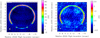 |
Fig. 1 CO (3–2) (left) and HCN (4–3) (right) line areas, as observed in Saturn with ALMA on May 25, 2018. |
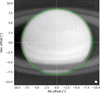 |
Fig. 2 Continuum image of Saturn at 345 GHz. The green line represents the position of the one-bar pressure level which we adopt for our limb spectra extraction. The east-west convention used is the planetary convention (left for west and right for east). The pixel size is 0.2″. |
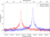 |
Fig. 3 CO spectra extracted from the image at the eastern (red line) and western (blue line) equator. The black vertical line indicates the rest frequency of the CO (3–2) line. |
3.2 Spectral fitting and Doppler shift derivation
We measured the Doppler shift of the CO and HCN lines at each position on the limb by fitting the line profile with the phenomenological spectral line profile described in Appendix B. To determine the parameters of the phenomenological profile, among which is the value of the Doppler shift, we used a Markov chain Monte Carlo (MCMC) procedure. The full procedure was initially developed to measure zonal winds in Jupiter’s stratosphere and is detailed in Cavalié et al. (2021). An example of spectral line fit is shown in Fig. B.1. This procedure also allows us to obtain the uncertainties on the Doppler shifts.
3.3 Subtraction of the planet rotation
Finally, we used the radiative transfer model described in Cavalié et al. (2019) to model the spectral emission of the CO (3–2) and HCN (4–3) lines1 with the spectral and spatial resolutions of the ALMA observations at the positions as used for the extraction of the spectra from the data cube. The planet rotation was accounted for before the spatial convolution of the spectra to the synthetic beam resolution. For each spectrum we could thus measure the contribution of the planet rotation by measuring the shift of the centre of the line in the simulations.
Finally, we subtracted the contribution of the planet rotation from the measured Doppler shifts to derive the winds at each pointing on the limb. Repeating this procedure for each pointing, we were able to derive the wind profile as a function of latitude on the two planetary limbs (east and west). We note that all latitudes in this paper are planetocentric latitudes.
3.4 Saturn’s rotation period
In our radiative transfer simulation, we fixed the rotation period of Saturn to that of the rotation of the magnetic field (10 h 39 min 24 s), as determined by the Voyager measurements, based on the periodicity of Saturn’s kilometric radiation (SKR; Desch & Kaiser 1981). However, the rotation period of Saturn remains highly debated. Thirty years later, the Ulysse spacecraft, followed by Cassini, measured different periods for the SKR, varying over the course of a few months and between the north and south poles. These modulations in Saturn’s radio period are thought to be due to ionospheric phenomena (Chowdhury et al. 2022). Hence, the period of the SKR does not seem strictly related to the rotation period of Saturn’s interior, and other methods have since been used to derive it, such as the measurement of the gravity field (Helled et al. 2015; Militzer et al. 2019) or the seismology of the rings (Mankovich et al. 2019).
The magnitude of the winds we derive obviously depends on the rotation period we adopt. A difference of 6 min in the rotation period of 9.9 km s−1 represents a difference of about 100 m s−1 at the equator and of 50 m s−1 at 60° latitude. In Studwell et al. (2018), the authors performed a comparison of measurements of tropospheric zonal winds by the VIMS and ISS instruments on board Cassini as a function of Saturn’s rotation periods. They showed that using the Voyager rotation period of 10 h 39 min 24 s, the VIMS measurements (sensitive at 2000 mbar) and ISS measurements (sensitive at 300–500mbar) gave zonal winds almost eastward at all latitudes. When using the Cassini rotation period ~10h 33 min 24 s (Anderson & Schubert 2007; Read et al. 2009), the measured zonal winds were eastward at low and equatorial latitudes, and there were alternations between weak eastward and westward jets with amplitudes up to 100 m s−1 beyond this latitude range. We discuss how this uncertainty affects our results in Sect. 4.
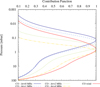 |
Fig. 5 Contribution functions (normalized to unity at maximum) of the CO (3–2) line in the atmosphere of Saturn. The solid blue, dashed, dotted, and dash-dotted curves represent examples of monochromatic contribution functions calculated at 0, 1, 2, and 4 MHz from the line centre, respectively. The solid red curve represents the wind contribution function (see text). |
3.5 Probed pressures
With the radiative transfer model we calculated the contribution functions of the lines at the spatial and spectral resolutions of the observations and at various frequencies from the line centre at the planetary limb. We used a CO vertical profile computed with the model of Hue et al. (2015, Hue et al. 2016), with an internal source of 1 ppb and an external flux of 2 × 106 cm−2 s−1, consistent with Cavalié et al. (2010).
A preliminary assessment of the HCN profile at the equator indicates that the bulk of HCN is restricted to pressures lower than ~0.5 mbar with a mole fraction of ~0.05 ppb. Detailed HCN profiles as a function of latitude will be reported in a subsequent paper (Fouchet et al. in prep.). For now, we used an HCN profile to calculate contribution functions. We then used these contribution functions to compute the wind’s contribution function (Lellouch et al. 2019), which represents the average of the monochromatic contribution functions, over the spectral interval used for the line fit, weighted by the local gradient of the simulated line. This result gives us an estimate of the pressure probed by the winds (i.e. the levels where the wind contribution function, normalized to its maximum, >0.5). Figure 5 shows that the CO winds probe pressures from 0.1 to 20 mbar. The results of the contribution function calculations for the HCN (4–3) (see Fig. 6) show that the HCN winds probe pressures from 0.01 to 0.5 mbar.
4 Results and discussion
4.1 CO and HCN winds and their uncertainties
The line-of-sight wind speeds measured from the CO observations on Saturn’s eastern and western limbs are displayed in Fig. 7. Latitudes between 44°S and 20°S are obscured by the rings (green area in the figure). In this area the measured spectral lines are very noisy, and thus not usable for wind measurements. Latitudes southwards of 44° S are mostly not visible because of sub-earth point was about 30°N (purple area in the figure). The average of the velocity error bars obtained from all spectra fitted northward of 20°S is about 15 m s−1. To these error bars we added quadratically two other sources of uncertainty. One is the link to the calibration of the planetary centre in the image, and which represents 25 m s−1 (see previous section). The other is the uncertainty due to the subtraction of a continuum baseline from each spectral line, and which represents on average 2 m s−1. The uncertainty resulting from calibrating the planet centre position is thus the dominant source of uncertainties in our wind retrievals.
Similar to CO, we used the HCN (4–3) data to measure the winds in the eastern and western limbs of Saturn. The results are presented in Fig. 8 with the same layout as for CO. We note that the HCN spectral line observations that we processed showed an overall shift of one spectral channel of 250 kHz (211.4 m s−1). We determined this shift from the spectra located at the central meridian (i.e. at high northern latitudes) where we assume the velocity to be zero. In what follows, and although we are unsure of the cause for this one-channel shift, we have applied a global subtraction of 211.4 m s−1 to the wind speeds derived from the HCN data. Since the S/N is lower compared to the CO observations, the HCN average velocity error obtained on all spectra fitted above 20°S is slightly higher (21 m s−1). The other systematic errors are the same as for CO and were added quadratically.
In these two wind measurement results, the red and blue curves represent the winds measured on the line of sight on the eastern and western limb of Saturn, respectively. In the 0.01-0.5 and 0.1-20 mbar pressure ranges probed respectively by the HCN and CO observations, we find a strong eastward (pro-grade) jet from 20° S to 25°N. Between 25°N and ~60°N, we find a global westward wind between 0.1 and 20 mbar from the CO data. The HCN data, which probe slightly lower pressures, do not show such a global westward wind. At even higher latitudes, in the HCN winds, we see a stronger variability, with westward jets around 60°N and at 71°N, which we discuss further in Sect. 4.4.
To make a comparison with the tropospheric zonal wind measurements, we calculated the zonal component of the CO and HCN wind measurements, assuming that the meridional component is negligible. Recent GCM simulations by Bardet et al. (2021) indicate that meridional winds are indeed weaker than zonal winds by (typically) a factor of 20 (if no large cyclone or anticyclone is present). We thus deprojected the line-of-sight winds on the zonal axis by dividing all wind speeds by the cosine of the sub-Earth latitude. The results for CO and HCN are shown in Fig. 9 and compared to the measurements of García-Melendo et al. (2011) from CassiniαSS cloud-tracking for two pressure layers.
4.2 Equatorial zone and SSAO
Our main discovery is the observation of a broad super-rotating jet between 20° S and 25°N that is very well correlated in shape, direction, and magnitude with the jet measured in the upper troposphere and lower stratosphere. This jet thus probably extends from 2000-0.01 mbar, according to our observations. Figure 10 shows that the average jet speed in the 0.01–20 mbar pressure range is 290 ± 30 m s−1 and that the average speed of this jet decreases overall from the troposphere to the upper stratosphere.
Fletcher et al. (2017) attempted to estimate the vertical structure of the large equatorial jet from temperature measurements. Using the thermal wind equation and by integrating from the 500 mbar pressure level to lower pressures, while considering observed tropospheric wind measurements at 500 mbar as the initial condition, they obtained a westward jet of more than 200 m s−1 at the 1 mbar level for 2016, which the authors judged unrealistic. This is indeed in total disagreement with our observations. This discrepancy might be explained by the rather coarse vertical resolution of the available temperature measurements, combined with a gap in sensitivity between 5 and 80 mbar. In contrast, when they integrated the thermal wind equation starting from the 5 mbar pressure level (considering a zero initial condition on the winds) to lower pressures (within the range of validity of the stratospheric thermal field measurements), they obtained, for the same date (2016), a wind speed of −200 m s−1 around 1 mbar relative to that at 5 mbar (Fig. S8 in the supplementary file of Fletcher et al. 2017).
Wind speeds derived from applying the thermal wind equation are very sensitive to errors in the vertical and latitudinal temperature gradients and suffer from large uncertainties (see also Benmahi et al. 2021). In contrast, our wind measurements derived from CO between 0.1 and 20 mbar now provide a direct constraint on the mean zonal wind over this pressure range. Given that the SSAO is characterized by wind extrema separated by approximately a decade of pressure, our CO winds thus roughly correspond to the mean zonal wind around which the SSAO oscillates. This value is 290±30 m s−1. Combined with the wind shear derived from Fletcher et al. (2017) and Guerlet et al. (2018), reaching on average −150 m s−1 between two wind extrema, our results imply that the absolute SSAO winds are always eastward. This holds true even when taking into account the uncertainty in Saturn’s rotation period (−100 m s−1 for a 6 min faster rotation rate). This behaviour is different from the QBO and the SAO on Earth, where the wind speeds oscillate around approximately zero.
Finally, the results from HCN indicate the corresponding SSAO phase at 0.01–0.5 mbar at the time of our observations. The HCN-derived winds appear to be marginally larger than the mean zonal wind, which is consistent with a positive phase of the SSAO at 0.01–0.03mbar observed in 2015 by Guerlet et al. (2018).
Another particularity of the broad equatorial jet between 20° S and 25 °N is that it is not symmetrical in speed around the equator in both the CO and HCN observations. Between the equator and 25°N, the average velocity of the jet is about 210 m s−1, while between the equator and 20°S its average velocity exceeds 300 m s−1 with apeak of more than 350 m s−1 at 10°S. In the results of García-Melendo et al. (2011) in the 60-250 mbar and 350–500 mbar ranges, we find a similar asymmetry, but in opposite hemispheres. The fact that the Cassini observations were collected half a Saturnian year from our ALMA observations could indicate that the reversal in the asymmetry of the jets at ±10° could be a seasonal effect. Global climate modelling of Saturn’s stratosphere shows a strong seasonality in the strength of the jets located at 20°N and 20°S, with faster jets obtained in the winter tropics, correlated with ring shadowing (Bardet et al. 2021). This might be driven by the seasonal inter-hemispheric circulation (Bardet et al. 2022): during solstice seasons the modelled seasonal inter-hemispheric circulation encounters the mid-latitude Rossby wave breaking zone, which causes the deviation of the main branch of this inter-hemispheric circulation underneath the ring shadowing. At these seasons, because the main westward momentum was transferred at the equatorial mean flow, the inter-hemispheric circulation mainly transports eastward momentum to winter low latitudes, which forces the mean atmospheric flow and produces an intense eastward jet at 15–20° in the model. To summarize, a more intense eastward jet is obtained in the GCM simulations in the winter hemisphere, similarly to the work reported here. Hence, the observed jet asymmetries could support the modelling results.
The GCM simulations of Saturn’s atmosphere developed by Spiga et al. (2020) and Bardet et al. (2021) produce mid-latitudinal jets in relatively good agreement with the tropospheric observations. However, the large equatorial eastward jet is poorly reproduced in the troposphere and stratosphere. It is an order of magnitude slower and is not as broad as in the Cassini and ALMA observations. This jet being probably the result of an acceleration due to the convergence of the eddy momentum towards the equator, Spiga et al. (2020) conclude that the effects of this acceleration caused by waves and eddies are underestimated in the GCM model. Further modelling work is needed to improve this aspect and assess the impact of a more realistic tropospheric wind on the SSAO.
In the equatorial zone, the main difference between tropospheric and stratospheric measurements then resides in the presence of a narrow equatorial peak only seen between 60 and 500 mbar in the troposphere (see Fig. 9). Cassini/ISS observations in the MT and CB filters (Barbara & Del Genio 2021; García-Melendo et al. 2011) revealed a very intense narrow jet at the equator in the latitude range from 3°S to 3°N. Compared to the average winds of the large equatorial jet that spans between 20°S and 25°N, this narrow jet is relatively weak in CB observations at 350–500mbar pressure, but it is very intense in MT observations at 60–250 mbar pressure (Fig. 9). Our CO observations between 0.1 mbar and 20 mbar do not reveal any sign of a narrow intense jet at the equator. This is quite surprising as we expected to detect this peak which could be related to the SSAO.
That we do not see any evidence for such a peak superimposed over the broad eastward jet in the CO data may simply result from the large vertical extent of the CO wind contribution function (Fig. 5), which may cancel any contribution of the SSAO by encompassing opposite phases of the SSAO. Interestingly, the HCN wind contribution function is more peaked than the CO one (around the peak level), and looking carefully at the HCN wind profile (Figs. 8 and 9), we detect a narrow local minimum in the velocities between 5°S and 1 °N, with a negative amplitude of −50 ± 20 m s−1 with respect to the average between 10°S and 10°N shown in Fig. 10. This is consistent with the order of magnitude of the SSAO peaks, according to Guerlet et al. (2018).
 |
Fig. 7 Line-of-sight wind speeds derived from the CO (3–2) observations. The speeds measured at the eastern and western limbs are displayed in red and blue, respectively. |
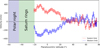 |
Fig. 8 Line-of-sight wind speeds derived from the HCN (4–3) observations. The layout is the same as in Fig. 7. |
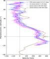 |
Fig. 9 Zonally averaged eastward winds from CO and HCN observations compared with the García-Melendo et al. (2011) measurements. The eastward winds for HCN and CO are obtained by averaging the winds between the two limbs of the planet, i.e. |

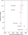 |
Fig. 10 Averages of the zonal wind speed in the broad eastward equatorial jet between 10°S and 10°N, excluding latitudes between 3°S and 3°N from the Cassini/VIMS, Cassini/ISS (CB and MT filters), and ALMA (CO and HCN) data. |
4.3 Northern hemisphere mid-latitudes
Between 25°N and 60°N, we find tentative evidence for the first time of a global westward wind with an average speed of −50 ± 30 m s−1 in both limbs from the CO data (Fig. 9). Moreover, our HCN and CO wind measurements show that the tropospheric eastward jet seen at 42°N (Fig. 9) has completely vanished in the stratosphere. We also find westward velocities with HCN between 25°N and 50°N, but only marginally. It is noteworthy that some of the only features that could be tracked in Saturn’s stratosphere were the hot vortices, nicknamed the beacons, that were formed in the stratosphere following Saturn’s Great White Spot of 2010–2011. Fletcher et al. (2012) notably found that the post-merger beacon had a westward motion of 1.6 ± 0.2° per day (i.e. ~−15 m s−1 at ~35°N). These observations are thus consistent with the average wind obtained in this latitude range from our data.
In Fig. 8, the eastward and westward peaks seen in the HCN winds at 61°N, 55°N, 50°N, and 45°N at the western limb and at 55°N, 59°N, and 67°N at the eastern limb, and that have amplitudes exceeding 100 m s−1 do not correspond to a zonal circulation because they do not have a symmetrical counterpart on the other limb. In this latitudinal range in the troposphere, the dynamics are often perturbed by the presence of vortices and other instabilities due to meridional shear of the upper tropospheric jets at mid-latitudes (see Trammell et al. 2014). Above this pressure level, in the stratosphere, and at these latitudes, the question is whether a circulation similar to that observed by Trammell et al. (2014) in the upper troposphere occurs and whether or not a 150 m s−1 velocity is realistic for these hypothetical eddies. This could explain our results of non-zonal peaks in the eastern and western limbs around 60°N. In Fig. 9, the peaks around 60°N and 65°N, both slightly around 100 ms−1, are not significant because they result from the average of the non-zonal peaks (see Fig. 8) at 61°N in the western limb and 55°N, 59°N, and 67°N in the eastern limb. Waves are another candidate for non-zonal wind components. For instance, observations of the hexagonal wave structure at 78°N by Antuñano et al. (2015) showed a perturbation of 30 m s−1 in the upper troposphere, which seems to be consistent with a ~0.5 K amplitude in the tropospheric thermal structure (as determined from Cassini/CIRS by Fletcher et al. 2018). By extrapolation, a non-zonal wind of 50–100 m s−1 can be associated with a thermal wave amplitude of 1–2 K.
4.4 A retrograde auroral jet at 71° N as in Jupiter?
At polar latitudes we cannot identify any significant jet from the CO measurements. However, in the HCN observations, we find a strong and narrow westward jet at 71 ± 2°N with a speed higher than 200 m s−1 on the western limb and between 150 and 200 m s−1 on the eastern limb. The peak sensitivity of the HCN winds is at 0.3 mbar, which represents ~ 100 km above the peak sensitivity of the CO winds, possibly explains the difference between the two wind profiles at this latitude.
We tentatively infer that this jet bears similarities to the auroral jets detected in Jupiter by Cavalié et al. (2021). They found polar jets correlated with the statistical position of the northern and southern main oval of the aurora. The two jets were non-zonal, owing to the tilt of the magnetic field axis with respect to the planet rotation axis, and they were found in counter-rotation. Knowing that the magnetic axis of Saturn is aligned with the rotation axis (Smith et al. 1980; Ness et al. 1981; Connerney et al. 1982; Dougherty et al. 2005, 2018), the northern and southern auroral ovals are well centred around the poles (Lamy et al. 2018). The fact that the speed of the 71°N jet is, within error bar, the same on both limbs (i.e. that it could be purely zonal) is not inconsistent with an auroral origin given the geometry of Saturn’s auroral ovals, although a non-auroral origin is also possible. We cannot directly compare the position of this jet with the position of the northern main oval of Saturn because we lack simultaneous observations of the northern aurora. If we now consider the average position of the northern auroral oval between February 2017 and September 2017 as observed with the Hubble Space Telescope (HST; Lamy et al. 2018), we can tentatively make such a comparison (see Fig. 11). We deduce from this that the jet at 71°N is indeed located in the area of the mean position of the northern auroral oval.
We do not know the vertical extent of Saturn’s stratospheric putative auroral jet at 71°N towards very high altitudes, but the case of Jupiter shows us that these jets can exist at ionospheric pressures with velocities ranging from 1 to 2 km s−1 (Rego et al. 1999; Stallard 2001; Stallard et al. 2003). The auroral jets in Jupiter’s stratosphere may be caused by the thermal gradient between the auroral region heated by electron precipitation and the cooler surrounding region and/or ion drag if the ionosphere penetrated down to stratopheric levels in the auroral region. If the jet we detect at 71°N in Saturn’s stratosphere is indeed an auroral jet, it could have the same origin as Jupiter’s jets.
5 Conclusion
In this paper we have obtained the first direct wind measurements in Saturn’s stratosphere using heterodyne spectroscopy in the millimetre range with ALMA observations carried out on May 25, 2018, using a similar method to that in Cavalié et al. (2021). We have derived the Doppler shifts caused by the stratospheric winds on the CO and HCN spectral lines, both observed at very high spectral and spatial resolutions. The main results can be summarized as follows:
We have derived two wind profiles as a function of latitude assuming the Voyager rotation period of Saturn as a reference for solid rotation. These profiles probe the stratosphere at 0.01–0.5 mbar for HCN and at 0.1–20 mbar for CO;
In the equatorial zone we have discovered that the broad super-rotating jet observed for decades in the troposphere extends to the upper stratosphere with an average speed of 290 ± 40 m s−1 between 0.01 and 20 mbar. It thus extends (at least) from 2000mbar, as observed by Cassini/VIMS (Studwell et al. 2018), to 0.01 mbar, as now observed by ALMA;
The broad super-rotating equatorial jet is not symmetrical with respect to the equator. Its southern branch, around 12°S, blows about 100 m s−1 faster than the northern one. As this asymmetry is opposite to the one observed in the troposphere in the Cassini data of 2004–2008 (i.e. about half a Saturnian year before the ALMA observations), it may be seasonal with the strongest branch of the jet residing in the winter hemisphere. This feature seems to be in agreement with the GCM predictions of Bardet et al. (2022). Further observations are required for confirmation;
The winds derived from CO do not show any evidence for the signature of the SSAO at the equator, as we observe no departure from the global trend of the broad super-rotating equatorial jet. Because the CO winds probe a large vertical region of the stratosphere, from 0.1 to 20 mbar, they mix various phases of the SSAO resulting in a near-zero average for the SSAO winds;
On the contrary, we tentatively detect a narrow westward peak with a velocity of −50 ± 30 m s−1 on top of the broad super-rotating equatorial jet. This may be the signature of the SSAO at 0.3 mbar, where the peak of the HCN wind contribution function resides;
Even the strongest retrograde branch of the SSAO of Fletcher et al. (2017), with a (relative) speed of ~−200 ms−1, would not reverse the wind direction at the equator, given the equatorial average speed of more than 250 m s−1 we retrieve from the CO and HCN observations. The winds in the region of the SSAO thus remain always eastward;
We find tentative evidence for a broad westward wind at mid-northern latitudes with an average speed of −50 ± 30 ms−1 in the CO winds. It is only marginally seen in the HCN winds. This result also shows that the tropospheric eastward jet seen at 42°N has completely vanished;
At northern polar latitudes, we detected a possible jet of about 200 m s−1 that is correlated with the position of Saturn’s northern main auroral oval. We have established this correlation using the mean position of Saturn’s northern auroral oval as observed in 2017 from HST observations (Lamy et al. 2018). This jet is westward and thus in counter-rotation, as are the stratospheric auroral jets found in Jupiter by Cavalié et al. (2021).
An observational follow-up is now necessary to characterize the seasonal variability of the northern and southern branches of the broad super-rotating equatorial jet, to study the vertical and temporal evolution of the SSAO, and to investigate for an auroral circulation pattern that could be similar to the Jupiter case. With the northern fall equinox nearing, the southern hemisphere is progressively more and more observable and measurements of the winds from the southern mid-latitudes down to the south pole will indicate whether the southern winds share similarities with the northern ones presented in this paper.
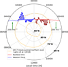 |
Fig. 11 Line-of-sight jet speeds and directions north of 68°N compared to the average position of Saturn’s northern main auroral oval in 2017, as observed by Lamy et al. (2018). The red and blue arrows represent the speeds on the eastern and western limbs, respectively. The strongest winds occur around 74°N on both limbs. The green arrow key at the top right of the plot indicates a speed of 200 m s−1. |
Acknowledgements
This work was supported by the Programme National de Planétologie (PNP) of CNRS/INSU and by CNES. This paper makes use of the following ALMA data: ADS/JAO.ALMA#2017.1.00636.S. ALMA is a partnership of ESO (representing its member states), NSF (USA) and NINS (Japan), together with NRC (Canada), MOST and ASIAA (Taiwan), and KASI (Republic of Korea), in cooperation with the Republic of Chile. The Joint ALMA Observatory is operated by ESO, AUI/NRAO and NAOJ. B. Benmahi thanks Laurent Lamy for providing the UV brigthness data of Fig. 11. D. Bardet is supported by a European Research Council Consolidator Grant (under the European Union’s Horizon 2020 research and innovation programme, grant agreement No 723890) at the University of Leicester. Bardet and Guerlet acknowledge funding from Agence. National de la Recherche (ANR), project EMERGIANT ANR-17-CE31-0007.
Appendix A Pointing offset calibration
The wind measurements in this paper require an accurate determination of the true position of the centre of the planet in the ALMA image. With an equatorial rotation speed of about ~ 10 km/s and an apparent size of 18″, an error of 0.1″ at the centre of Saturn would result in an error of about 130 m/s on the velocities. In this section, we detail our method to determine the offset of the planet centre from the image centre in the spectral cube, in order to calibrate it out.
We first defined an offset grid ∆x ∆y that has a dimension of 0.6″ × 0.6″ with a sampling of 0.01″ around the centre of the image. This grid is used to compare our limb continuum model with the limb continuum observed using the χ2 method at each point (x, y) of the offsets grid.
We performed our continuum calculations with the radiative transfer of Cavalié et al. (2019), which account for the ellipsoidal geometry of the planet. We assume an altitude-latitude temperature field measured by Cassini/CIRS in 2017, an He mole fraction 0.118 (Conrath & Gautier 2000; Koskinen & Guerlet 2018), and a CH4 mole fraction of 0.047 (Fletcher et al. 2009b). The PH3 meridional distribution is taken from Fletcher et al. (2009a) and we adopt the vertical profile of NH3 from Davis et al. (1996). The model accounts for the beam convolution.
After the comparisons we obtain a χ2 map of the same dimension as the offset grid. We then compute the probability function map which is given by  , where i and j are the indices of (x, y) points in the offset grid,
  is computed at each (x, y) point in the offset grid, and κ is a normalization factor computed to ensure
  .
.
We used several methods to compute the planet centre offset. At each point of the offset grid 1) we compared the continuum of the whole planetary disk between the observations and our radiative transfer model, 2) we limited the comparison of the continuum between the data and the model to the limb positions, and 3) we computed the mean continuum at the limb from the data and compared the continuum at each position with this mean value. There is no continuum model involved with this method. For methods 1 and 2, we then looked for the position in the chosen offset grid leading to the maximum correlation coefficient. For method 3, we computed the χ2 for each point of the offset grid and looked for its minimum.
Methods 1 and 2 are affected by the same bias. The continuum map observed is not symmetrical with respect to the planet rotation axis, and higher continuum values are systematically found on the eastern side of the planet (see figure 2). As a result, methods 1 and 2 always give offsets to the east which are unrealistic.
Method 3 assumes that there is limited continuum variability as a function of latitude at the limb, and we thus look for the flattest continuum as a function of the position on the limb. This method provides the most probable offset (xbest, ybest) of the planet centre position. With this method we find xbest = 0.11″ and ybest = 0.18″.
Method 3 also enables us to estimate the uncertainty on the wind speed derivation caused by the uncertainty of the planet centre offset. Because the rotation axis of the planet is aligned with the y-axis of the image, the wind speed uncertainty due to the uncertainty on the real position of the centre of the planet is only caused by the uncertainty on the derivation of xbest. To evaluate it we computed the probability function presented in Fig. A.1, and we fitted it with a two-dimensional Gauss probability density distribution given by the expression
 (A.1)
(A.1)
where r is the correlation coefficient between x and y; x0 and y0 are respectively the density of the average probabilities of the real position of the centre of the planet; and σx and σy are respectively the standard deviations of the distribution of the real position of the centre of the planet following x and y.
We find σx = 0.02″. At the equator, this standard deviation represents an uncertainty on the wind velocities of about 25 m/s. This uncertainty is quadratically added to the other uncertainties described in the paper.
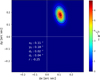 |
Fig. A.1 Probability function map of the planet centre offset. The contour lines represent the best fit with the function ϕ(x, y) described in the text. |
Appendix B MCMC prior function
Similarly to Cavalié et al. (2021), the function that describes the lineshape we used to fit the observed spectral lines is given by
 (B.1)
(B.1)
This profile is composed of five mathematical functions defined in ℝ ∀ α ≥ 0. Each function has an effect on the shape of the line profile:
 is a Gaussian like function which allows us to produce the central zone of a highly convolved spectral line (low spectral resolution for example);
 is a Lorentz-like function that reproduces narrow peaks with broad line wings;
 is the sum of an absolute power function and a modified Lorentzian function that controls the amplitude of the spectral line;
(Γ2 + (v − ν0)2 + 1)−1 is a modified Lorentz function that allows us to control the amplitude in the wings of the spectral line;
A is a normalization amplitude in Jy/beam.
This profile contains several parameters, namely v0, Γ, γ, σ, δ, α, β, and the amplitude A. The parameters δ, σ have fixed values, which we have determined through several numerical tests to obtain a very narrow spectral line with broad wings. The parameter δ allows us to obtain a very peaked line with very attenuated wings, and the parameter a allows us to raise the wings of the line. Finally, the parameter σ allows us to control the width of the Gaussian function. Contrary to Cavalié et al. (2021), we fix the value of α and we fit β.
We set the following values for these fixed parameters as α = 3.0, δ = 3.0, and σ = 0.202 [GHz]. The parameters v0, Γ,γ, β, and the amplitude A are parameters we adjust according to the observed spectral line. To fit the CO and HCN lines observed with ALMA more efficiently, we were able to restrain the parameter space after numerical tests to the following:
v0 ∈ [vmax − 1 MHz; vmax + 1MHz] because v0 is close to the frequency where the amplitude of the line is maximum;
Γ ∈ [0.0001; 0.1] en GHz;
β ∈ [5;40];
γ ∈ [0.04; 2.2];
A ∈ [Amax − 40%; Amax + 40%], where Amax (in Jy/beam) is the maximum amplitude of the observed spectral line.
With this set of parameters we can fit any observed spectral line of our data. Figure B.1 presents a typical example of such a fit and its residuals.
To perform this fit of all the parameters, especially v0 which is used for the wind speed derivation, we used the emcee Python module developed by Foreman-Mackey et al. (2013), which implements the MCMC method and uses the Metropolis-Hastings algorithm. The set-up of the observed spectral line fitting is characterized by 120 Markov chains and 1000 iterations. These two parameters were determined after several trials when measuring the burn-in size. We found that the Markov chains converge after 200–400 iterations on average for all spectral lines. The choice of 1000 iterations then ensures a convergence of the Markov chains in all cases.
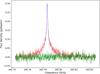 |
Fig. B.1 Typical CO line observed at Saturn’s limb (red line) with its associated best fit using the profile of equation B.1 (blue line) and the residuals (green line). |
References
- Anderson, J. D., & Schubert, G. 2007, Science, 317, 1384 [NASA ADS] [CrossRef] [Google Scholar]
- Antuñano, A., del Río-Gaztelurrutia, T., Sánchez-Lavega, A., & Hueso, R. 2015, J. Geophys. Res.: Planets, 120, 155 [CrossRef] [Google Scholar]
- Baines, K. H., Delitsky, M. L., Momary, T. W., et al. 2009, Planet. Space Sci., 57, 1650 [NASA ADS] [CrossRef] [Google Scholar]
- Barbara, J. M., & Del Genio, A. D. 2021, Icarus, 354, 114095 [Google Scholar]
- Bardet, D., Spiga, A., Guerlet, S., et al. 2021, Icarus, 354, 114042 [Google Scholar]
- Bardet, D., Spiga, A., & Guerlet, S. 2022, Nat. Astron. 6, 804 [NASA ADS] [CrossRef] [Google Scholar]
- Benmahi, B., Cavalié, T., Greathouse, T. K., et al. 2021, A&A, 652, A125 [NASA ADS] [CrossRef] [EDP Sciences] [Google Scholar]
- Butchart, N. 2014, Rev. Geophys., 52, 157 [NASA ADS] [CrossRef] [Google Scholar]
- Cavalié, T., Billebaud, F., Dobrijevic, M., et al. 2009, Icarus, 203, 531 [NASA ADS] [CrossRef] [Google Scholar]
- Cavalié, T., Hartogh, P., Billebaud, F., et al. 2010, A&A, 510, A88 [NASA ADS] [CrossRef] [EDP Sciences] [Google Scholar]
- Cavalié, T., Hue, V., Hartogh, P., et al. 2019, A&A, 630, A87 [NASA ADS] [CrossRef] [EDP Sciences] [Google Scholar]
- Cavalié, T., Benmahi, B., Hue, V., et al. 2021, A&A, 647, A8 [NASA ADS] [CrossRef] [EDP Sciences] [Google Scholar]
- Choi, D. S., Showman, A. P., & Brown, R. H. 2009, J. Geophys. Res.: Planets, 114, E04007 [Google Scholar]
- Chowdhury, M. N., Stallard, T. S., Baines, K. H., et al. 2022, Geophys. Res. Lett., 49, e2021GL096492 [CrossRef] [Google Scholar]
- Connerney, J. E. P., Ness, N. F., & Acuña, M. H. 1982, Nature, 298, 44 [NASA ADS] [CrossRef] [Google Scholar]
- Conrath, B. J., & Gautier, D. 2000, Icarus, 144, 124 [NASA ADS] [CrossRef] [Google Scholar]
- Davis, G. R., Griffin, M. J., Naylor, D. A., et al. 1996, A&A, 315, L393 [NASA ADS] [Google Scholar]
- Del Genio, A. D., Achterberg, R. K., Baines, K. H., et al. 2009, in Saturn from Cassini-Huygens, eds. M. K. Dougherty, L. W. Esposito, & S. M. Krimigis, 113 [CrossRef] [Google Scholar]
- Desch, M. D., & Kaiser, M. L. 1981, Geophys. Res. Lett., 8, 253 [NASA ADS] [CrossRef] [Google Scholar]
- Dougherty, M. K., Achilleos, N., Andre, N., et al. 2005, Science, 307, 1266 [NASA ADS] [CrossRef] [Google Scholar]
- Dougherty, M. K., Cao, H., Khurana, K. K., et al. 2018, Science, 362, aat5434 [NASA ADS] [CrossRef] [Google Scholar]
- Ebdon, R. A., & Veryard, R. G. 1961, Nature, 189, 791 [Google Scholar]
- Flasar, F. M. 2005, Science, 307, 1247 [NASA ADS] [CrossRef] [Google Scholar]
- Fletcher, L. N., Orton, G. S., Teanby, N. A., & Irwin, P. G. J. 2009a, Icarus, 202, 543 [NASA ADS] [CrossRef] [Google Scholar]
- Fletcher, L. N., Orton, G. S., Teanby, N. A., Irwin, P. G. J., & Bjoraker, G. L. 2009b, Icarus, 199, 351 [NASA ADS] [CrossRef] [Google Scholar]
- Fletcher, L. N., Hesman, B. E., Achterberg, R. K., et al. 2012, Icarus, 221, 560 [Google Scholar]
- Fletcher, L. N., Guerlet, S., Orton, G. S., et al. 2017, Nat. Astron., 1, 765 [Google Scholar]
- Fletcher, L. N., Orton, G. S., Sinclair, J. A., et al. 2018, Nat. Commun., 9, 3564 [NASA ADS] [CrossRef] [Google Scholar]
- Foreman-Mackey, D., Hogg, D. W., Lang, D., & Goodman, J. 2013, PASP, 125, 306 [Google Scholar]
- Fouchet, T., Guerlet, S., Strobel, D. F., et al. 2008, Nature, 453, 200 [Google Scholar]
- Fouchet, T., Moreno, R., Cavalié, T., et al. 2018, CBET 4535 [Google Scholar]
- Garcia, R. R. 2000, in Atmospheric Science Across the Stratopause, Geophys. Monogr. Ser., 123, 161 [CrossRef] [Google Scholar]
- García-Melendo, E., Pérez-Hoyos, S., Sánchez-Lavega, A., & Hueso, R. 2011, Icarus, 215, 62 [CrossRef] [Google Scholar]
- Guerlet, S., Fouchet, T., Bézard, B., Flasar, F. M., & Simon-Miller, A. A. 2011, Geophys. Res. Lett., 38, L09201 [Google Scholar]
- Guerlet, S., Fouchet, T., Spiga, A., et al. 2018, J. Geophys. Res.: Planets, 123, 246 [NASA ADS] [CrossRef] [Google Scholar]
- Helled, R., Galanti, E., & Kaspi, Y. 2015, Nature, 520, 202 [NASA ADS] [CrossRef] [Google Scholar]
- Hue, V., Cavalié, T., Dobrijevic, M., Hersant, F., & Greathouse, T. K. 2015, Icarus, 257, 163 [NASA ADS] [CrossRef] [Google Scholar]
- Hue, V., Greathouse, T. K., Cavalié, T., Dobrijevic, M., & Hersant, F. 2016, Icarus, 267, 334 [NASA ADS] [CrossRef] [Google Scholar]
- Koskinen, T. T., & Guerlet, S. 2018, Icarus, 307, 161 [NASA ADS] [CrossRef] [Google Scholar]
- Kuroda, T., Medvedev, A. S., Hartogh, P., & Takahashi, M. 2008, Geophys. Res. Lett., 35, L23202 [NASA ADS] [CrossRef] [Google Scholar]
- Lamy, L., Prangé, R., Tao, C., et al. 2018, Geophys. Res. Lett., 45, 9353 [NASA ADS] [CrossRef] [Google Scholar]
- Lellouch, E., Gurwell, M. A., Moreno, R., et al. 2019, Nat. Astron., 3, 614 [NASA ADS] [CrossRef] [Google Scholar]
- Leovy, C. B., Friedson, A. J., & Orton, G. S. 1991, Nature, 354, 380 [Google Scholar]
- Mankovich, C., Marley, M. S., Fortney, J. J., & Movshovitz, N. 2019, ApJ, 871, 1 [NASA ADS] [CrossRef] [Google Scholar]
- Militzer, B., Wahl, S., & Hubbard, W. B. 2019, ApJ, 879, 78 [Google Scholar]
- Muders, D., Wyrowski, F., Lightfoot, J., et al. 2014, in Astronomical Data Analysis Software and Systems XXIII, eds. N. Manset, & P. Forshay, ASP Conf. Ser., 485, 383 [NASA ADS] [Google Scholar]
- Ness, N. F., Acuña, M. H., Lepping, R. P., et al. 1981, Science, 212, 211 [NASA ADS] [CrossRef] [Google Scholar]
- Orton, G. S., Friedson, A. J., Caldwell, J., et al. 1991, Science, 252, 537 [Google Scholar]
- Orton, G. S., Yanamandra-Fisher, P. A., Fisher, B. M., et al. 2008, Nature, 453, 196 [Google Scholar]
- Reed, R. J. 1965, J. Atmos. Sci., 22, 331 [NASA ADS] [CrossRef] [Google Scholar]
- Reed, R. J., Campbell, W. J., Rasmussen, L. A., & Rogers, D. G. 1961, J. Geophys. Res., 66, 813 [Google Scholar]
- Read, P. L., Dowling, T. E., & Schubert, G. 2009, Nature, 460, 608 [NASA ADS] [CrossRef] [Google Scholar]
- Rego, D., Achilleos, N., Stallard, T., et al. 1999, Nature, 399, 121 [Google Scholar]
- Sánchez-Lavega, A., Hueso, R., Pérez-Hoyos, S., Rojas, J. F., & French, R. G. 2004, Icarus, 170, 519 [CrossRef] [Google Scholar]
- Showman, A. P., Ingersoll, A. P., Achterberg, R., & Kaspi, Y. 2018, in Saturn in the 21st Century, eds. K. H. Baines, F. M. Flasar, & N. Krupp, & T. Stallard, 295 [CrossRef] [Google Scholar]
- Smith, E. J., Davis, L., Jones, D. E., et al. 1980, Science, 207, 407 [NASA ADS] [CrossRef] [Google Scholar]
- Spiga, A., Guerlet, S., Millour, E., et al. 2020, Icarus, 335, 113377 [Google Scholar]
- Stallard, T. 2001, Icarus, 154, 475 [NASA ADS] [CrossRef] [Google Scholar]
- Stallard, T. S., Miller, S., Cowley, S. W. H., & Bunce, E. J. 2003, Geophys. Res. Lett., 30, 1221 [Google Scholar]
- Studwell, A., Li, L., Jiang, X., et al. 2018, Geophys. Res. Lett., 45, 6823 [NASA ADS] [CrossRef] [Google Scholar]
- Trammell, H. J., Li, L., Jiang, X., et al. 2014, Icarus, 242, 122 [NASA ADS] [CrossRef] [Google Scholar]
The two fainter lines of the (4–3) triplet produce negligible contribution to the flux compared to the observation noise level, and neither line is detected or influences significantly the shape and amplitude of the main line.
All Figures
|
Fig. 1 CO (3–2) (left) and HCN (4–3) (right) line areas, as observed in Saturn with ALMA on May 25, 2018. |
| In the text | |
|
Fig. 2 Continuum image of Saturn at 345 GHz. The green line represents the position of the one-bar pressure level which we adopt for our limb spectra extraction. The east-west convention used is the planetary convention (left for west and right for east). The pixel size is 0.2″. |
| In the text | |
|
Fig. 3 CO spectra extracted from the image at the eastern (red line) and western (blue line) equator. The black vertical line indicates the rest frequency of the CO (3–2) line. |
| In the text | |
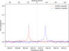 |
Fig. 4 Same as Fig. 3, but for HCN (4-3). |
| In the text | |
|
Fig. 5 Contribution functions (normalized to unity at maximum) of the CO (3–2) line in the atmosphere of Saturn. The solid blue, dashed, dotted, and dash-dotted curves represent examples of monochromatic contribution functions calculated at 0, 1, 2, and 4 MHz from the line centre, respectively. The solid red curve represents the wind contribution function (see text). |
| In the text | |
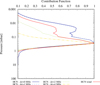 |
Fig. 6 Same as Fig. 5, but for the HCN (4–3) line. |
| In the text | |
|
Fig. 7 Line-of-sight wind speeds derived from the CO (3–2) observations. The speeds measured at the eastern and western limbs are displayed in red and blue, respectively. |
| In the text | |
|
Fig. 8 Line-of-sight wind speeds derived from the HCN (4–3) observations. The layout is the same as in Fig. 7. |
| In the text | |
|
Fig. 9 Zonally averaged eastward winds from CO and HCN observations compared with the García-Melendo et al. (2011) measurements. The eastward winds for HCN and CO are obtained by averaging the winds between the two limbs of the planet, i.e. |
| In the text | |
|
Fig. 10 Averages of the zonal wind speed in the broad eastward equatorial jet between 10°S and 10°N, excluding latitudes between 3°S and 3°N from the Cassini/VIMS, Cassini/ISS (CB and MT filters), and ALMA (CO and HCN) data. |
| In the text | |
|
Fig. 11 Line-of-sight jet speeds and directions north of 68°N compared to the average position of Saturn’s northern main auroral oval in 2017, as observed by Lamy et al. (2018). The red and blue arrows represent the speeds on the eastern and western limbs, respectively. The strongest winds occur around 74°N on both limbs. The green arrow key at the top right of the plot indicates a speed of 200 m s−1. |
| In the text | |
|
Fig. A.1 Probability function map of the planet centre offset. The contour lines represent the best fit with the function ϕ(x, y) described in the text. |
| In the text | |
|
Fig. B.1 Typical CO line observed at Saturn’s limb (red line) with its associated best fit using the profile of equation B.1 (blue line) and the residuals (green line). |
| In the text | |
Current usage metrics show cumulative count of Article Views (full-text article views including HTML views, PDF and ePub downloads, according to the available data) and Abstracts Views on Vision4Press platform.
Data correspond to usage on the plateform after 2015. The current usage metrics is available 48-96 hours after online publication and is updated daily on week days.
Initial download of the metrics may take a while.