


| Issue |
A&A
Volume 710, June 2026
|
|
|---|---|---|
| Article Number | A297 | |
| Number of page(s) | 20 | |
| Section | Catalogs and data | |
| DOI | https://doi.org/10.1051/0004-6361/202558131 | |
| Published online | 19 June 2026 | |
Ariel stellar characterisation
IV. Fundamental parameters of 18 hot stars in the Ariel mission candidate sample
1
Tartu Observatory, University of Tartu,
Observatooriumi 1,
Tõravere
61602,
Estonia
2
Space Research Institute, Austrian Academy of Sciences,
Schmiedlstrasse 6,
8042
Graz,
Austria
3
Institute for Theoretical and Computation Physics, Graz University of Technology,
Petersgasse 16,
8010
Graz,
Austria
4
Department of Physics and Astronomy G. Galilei, University of Padova,
Vicolo dell’Osservatorio 3,
35122,
Padova,
Italy
5
INAF – Osservatorio Astronomico di Padova,
Vicolo dell’Osservatorio 5,
35122
Padova,
Italy
6
Departament d’Astronomia i Astrofísica, Universitat de València,
Av. Vicent Andrés Estellés 19,
46100
Burjassot,
Spain
7
INAF – Osservatorio Astrofisico di Arcetri,
Largo E. Fermi 5,
50125
Firenze,
Italy
8
INAF – Osservatorio Astrofisico di Torino,
Via Osservatorio 20,
10020
Pino Torinese,
Italy
9
Instituto de Astrofísica de Canarias,
Calle Vía Láctea s/n
38206
La Laguna,
Santa Cruz de Tenerife,
Spain
10
Universidad de La Laguna,
Avda. Astrofísico Francisco Sánchez
38205
La Laguna,
Santa Cruz de Tenerife,
Spain
11
Institute for Space Astrophysics and Planetology INAF-IAPS,
Roma,
RM,
Italy
12
INAF – Osservatorio Astronomico di Roma,
Via Frascati 33,
00040
Monte Porzio Catone (RM),
Italy
13
Agenzia Spaziale Italiana, Space Science Data Center,
via del Politecnico snc,
00133
Rome,
Italy
14
Department of Physics and Astronomy, University College London,
Gower Street,
London,
WC1E 6BT,
UK
15
INAF – Osservatorio Astronomico di Palermo,
Piazza del Parlamento, 1,
90134
Palermo,
Italy
16
INAF – Osservatorio Astronomico di Brera,
Via E. Bianchi 46,
23807
Merate (LC),
Italy
17
Nicolaus Copernicus Astronomical Center, Polish Academy of Sciences,
ul. Rabiańska 8,
87-100
Toruń,
Poland
★ Corresponding author: This email address is being protected from spambots. You need JavaScript enabled to view it.
Received:
15
November
2025
Accepted:
27
April
2026
Abstract
Context. The characterisation of exoplanetary systems depends on the accurate determination of host star parameters. The Ariel mission will probe the atmospheres of a statistically significant sample of exoplanets, and so requires a precise characterisation of the stellar properties well before its launch in 2031. The homogeneous determination of stellar parameters for Ariel will enable both the optimisation of the final target list and set roots for a reliable interpretation of the formation and evolution of planetary systems. Such a homogeneous characterisation has thus far only been carried out for the cool (Teff ≲ 7000 K) host stars among the Ariel target candidates.
Aims. We present a uniform determination of fundamental stellar parameters for 18 hot stars (Teff ≳ 7000 K) in the Tier 1 candidate list of the Ariel mission candidate sample.
Methods. We adopted an iterative spectro-trigonometric approach optimised for high-temperature stars (Teff ≳ 7000 K). Highresolution spectra were analysed using the ZEEMAN code with χ2 minimisation, combining model fits to metal and Balmer lines. Surface gravity was refined using photometry-based radii and masses from stellar evolutionary tracks.
Results. We derived effective temperatures, surface gravities, projected rotational velocities, microturbulent velocities, overall metal-licities, iron abundances, stellar masses, and radii for our sample of 18 hot stars. Our results were validated against a set of benchmark stars previously presented in the literature, confirming that our methods yield results consistent with previous studies. This ensures an internally consistent parameter scale and maintains continuity across the transition from cool to hot stars within the Ariel sample.
Conclusions. The derived parameters provide an internally consistent basis for studying the link between stellar properties and planetary characteristics in intermediate-mass stars (1.5 < M < 2.32 M⊙). Building on our previous work on FGK host stars, we show that correlations between stellar mass, metallicity, and planetary radii also extend to early-type stars, and stellar properties influence the architecture of multi-planet systems.
Key words: methods: data analysis / techniques: spectroscopic / catalogs / stars: early-type / stars: fundamental parameters / planetary systems
© The Authors 2026
 Open Access article, published by EDP Sciences, under the terms of the Creative Commons Attribution License (https://creativecommons.org/licenses/by/4.0), which permits unrestricted use, distribution, and reproduction in any medium, provided the original work is properly cited.
This article is published in open access under the Subscribe to Open model. This email address is being protected from spambots. You need JavaScript enabled to view it. to support open access publication.
1 Introduction
In the context of planetary science beyond the Solar System, the host stars of exoplanetary systems have become central to our understanding of planets and their environments. Over the past decade, it has grown increasingly clear that the nature of planets, their origins, and their subsequent evolution cannot be fully addressed without considering their host stars. Accurate characterisation of exoplanet host stars is therefore essential for interpreting planetary systems and understanding the conditions under which planets form and evolve. This is particularly true in the field of exoplanetary atmospheres, where a coherent and complete characterisation of the host star is indispensable. Planetary parameters - for instance, the planetary radius, mass, and hence density and bulk elemental composition - depend on the corresponding stellar values (e.g. Johnson et al. 2010; Buchhave et al. 2014; Santos et al. 2017; Teske 2024; de Laverny et al. 2025). In addition, stellar activity can drive chemical changes in planetary atmospheres or even trigger planetary mass loss, further underscoring the importance of precise stellar characterisation (e.g. Segura et al. 2010; Vidotto et al. 2015; Johnstone et al. 2019; Gupta et al. 2023; Nicholls et al. 2023). To meet these challenges, the community has devoted significant effort to characterising the stars with known planetary systems. However, if the ultimate goal is to trace the formation and evolution of planets, the next step is to extend this effort to a populationwide scale. Such studies require stars and planets to be analysed in a homogeneous way, in order to eliminate systematic errors that arise from, for example, different spectroscopic pipelines or inconsistent photometry. Without this homogeneity, methodological offsets may mimic or obscure genuine astrophysical trends between stellar and planetary properties. Consistency across samples is therefore critical for robust statistical conclusions and for ensuring that observed correlations reflect astrophysics rather than analysis artefacts (e.g. Adibekyan et al. 2015, 2021; Magrini et al. 2022; Biazzo et al. 2022; da Silva et al. 2024; Filomeno et al. 2024). Building on this need for a large-scale stellar and planetary characterisation, the first space mission dedicated to a systematic atmospheric population survey will be the ESA M4 mission Ariel. Ariel will observe the atmospheres of roughly one thousand exoplanets, using a tiered survey strategy (Tinetti et al. 2018, 2022), with the goal of identifying the origins of different planetary classes and ultimately uncovering population-level trends that will advance our understanding of planetary formation and evolution.
To achieve such a significant goal, a precise and homogeneous determination of the stellar parameters is required well before launch in 2029 (Danielski et al. 2022). In fact, to optimise the scientific outcome of Ariel throughout its nominal mission lifetime, a thorough study of the Ariel candidate planetary systems needs to be performed beforehand. This task is essential for identifying key or compelling targets, as well as for increasing the diversity of the population in terms of both planetary atmospheric characteristics and host star properties. By expanding this diversity, we improve the chances of uncovering populationlevel trends in exoplanet atmospheres, while also placing these planetary atmospheres within a broader Galactic context. In this regard, we refer the reader to Cowan & Coull-Neveu (2025) for an overview of strategies to maximise Ariel’s survey yield, as well as a discussion of the caveats associated with selecting the final target list. The ‘Stellar Characterisation’ Working Group of the Ariel consortium has focused on the uniform determination of parameters for solar-like FGK stars, which represent the majority of the mission’s candidate sample. Magrini et al. (2022, hereafter M22) derived kinematical properties, effective temperatures, surface gravities, metallicities, microturbulent velocities, masses, and radii for 187 FGK stars using a combination of spectroscopic, photometric, and astrometric data. More recently, Tsantaki et al. (2025, hereafter T25) extended this analysis to fast-rotating FGK stars, presenting parameters for a total of 353 stars, which include both slow-rotating and fast-rotating stars, and additionally providing projected rotational and macroturbulent velocities. Ongoing efforts will further expand this work to cooler M-type stars (Maldonado et al., in prep.).
In this work, we present fundamental parameters for 18 stars with spectral types from early F to A (6800 < Teff < 9560 K). These stars, part of the Ariel Tier 1 Mission Candidate Sample (MCS, Edwards et al. 2019; Edwards & Tinetti 2022), have not yet been characterised by the Ariel Stellar Characterisation Working Group. This is because the methods developed for FGK stars in M22 and T25 are not directly applicable to hotter stars. The rapid rotation in A- and early F-type stars leads to significant line broadening and blending, complicating spectral analysis and reducing the precision of parameter estimation. To maintain continuity across the full sample, we benchmarked our procedure against M22 and T25 in the overlapping temperature regime (∼5000-7000K), where the spectro-trigonometric approach recovers consistent parameters.
Intermediate-mass stars serve as a testbed for planet formation theories, which offer competing predictions regarding occurrence rates: higher gas-giant frequencies due to massive protoplanetary discs (e.g. Kennedy & Kenyon 2008; Johnson et al. 2010) versus increased rarity due to rapid disc dispersal or less efficient inward migration (Reffert et al. 2015; Johnston et al. 2024). Extending internally consistent characterisation to our sample (M* ≥ 1.4 M⊙) also allows us to test physical scaling relations, such as the correlation between host-star metallicity and planet presence (Gonzalez 1997; Santos et al. 2004; Fischer & Valenti 2005) or the dependence of planetary radius inflation on stellar irradiation (Demory & Seager 2011; Weiss et al. 2013).
The sample is described in Sect. 2, followed by a description of our spectroscopic method and validation in Sect. 3. Results are presented in Sect. 4, with a discussion in Sect. 5 and conclusions in Sect. 6.
2 Sample of stars
We selected the 18 hottest stars from the MCS list that have high-quality spectra, except for HATS-701. The rest of the hot stars not included in this work are planned to be observed in current or future observing programmes. Figure 1 shows the Kiel diagram of stars analysed in this work together with stars analysed in M22 and T25.
We selected 23 stars for benchmarking our analysis with M22 and T25. The stars were selected randomly from a temperature range of 4900-7000 K and rotational velocities up to 70 km s−1 (Table B.2).
All the spectra were collected by the Ariel Science Consortium Working Group (SCWG) and were accessed via the Ariel Data Drive (Ariel DD). For most of the targets, high signal-tonoise ratio (S/N) spectra were available in public archives (e.g. the ESO Archive Science Portal). A few targets in the hot sample have spectra from successful proposals written by the working group.
We used high-resolution spectra (R ≃ 48 000-140 000) collected from the archives and instruments listed in Table 1. As shown by Tsantaki et al. (2025) and da Silva et al. (2024), the use of different high-resolution spectrographs introduces only minor variations in the derived stellar parameters. Since our spectra were obtained with the same instruments as in these previous works, we expect any such instrumental effects to be negligible within the quoted uncertainties.
Most spectral regions used in this analysis cover the wavelength range from ∼4300 Å to ∼6500 Å, with combined S/N values ranging from ≈100 to 1700. Table 1 summarises the spectra, including their sources, instruments, wavelength span used, and S/N values.
List of the 18 hot stars analysed in this work.
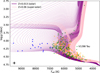 |
Fig. 1 Kiel diagram of analysed stars. Stars analysed in this work are shown as blue dots, those from M22 as orange stars, and those from T25 as green symbols. The two grids correspond to PARSEC isochrones with ages from 0.1 to 14 Ga, in steps of 0.05 Ga, at solar metallicity (Z = 0.013, in purple) and at super-solar metallicity (Z = 0.06, in pink). The cross in the lower left corner indicates representative 1σ uncertainties for this work (ΔTeff = 110 K and Δ log g = 0.04 dex). |
3 Method
In this work, we address the challenges of characterising hot stars. Our methodology follows the iterative spectro-trigonometric approach described in M22 and T25, which combines spectral synthesis, astrometry, and photometry to determine fundamental stellar parameters. We introduced several modifications to the spectroscopic analysis to accommodate the 18 earlier-type stars. Effective temperatures and surface gravities were initially constrained using Balmer-line fitting, which provides a consistent starting point for the analysis. Metal-line analysis was then performed to refine the remaining atmospheric parameters. Stellar masses were subsequently derived using Bayesian isochrone fitting, and bolometric magnitudes were obtained from Gaia Data Release 3 (DR3) parallaxes and broadband photometry. These quantities were combined to compute trigonometric surface gravities. The analysis then iterated: metal-line fitting was repeated with log g fixed to the trigonometric value, and Balmer-line fits were re-done to determine the final effective temperatures, until all parameters converged. This method allowed us to derive effective temperatures (Teff), surface gravities (log g), metallicities ([M/H]), iron abundances ([Fe/H]), microturbulent velocities (νmic), projected rotational velocities (ν sin i), masses, and radii for 18 hot stars. A schematic overview of the iterative spectro-trigonometric procedure is shown in Fig. 2.
3.1 Comparison to M22 and T25 methods
M22 employed an equivalent width (EW) method using MOOG, automated via the FAMA wrapper (Magrini et al. 2013). This approach, combined with MARCS model atmospheres, was optimised for FGK-type stars with v sin i up to ∼15 km s−1.
T25 extended the parameter space to faster rotators using spectral synthesis with the FASMA code2 (Tsantaki et al. 2018a,b), also based on MOOG. Their analysis relied primarily on iron lines selected by Tsantaki et al. (2018a). For Fe lines, the atomic data adopted were those from the Gaia-ESO survey (Heiter et al. 2021), as used in M22. For non-iron lines, the atomic data were taken from the Tsantaki et al. (2018a) line list.
In this work, we introduced the following methodological differences:
Hot stars exhibit significant line blending and rotational broadening, making fitting isolated iron lines or narrow spectral regions impractical. Instead, we fitted broader wavelength segments starting and ending in continuum regions.
The spectral regions used in this work differ from those in M22 and T25. The regions used are much broader, including many, often blended, spectral lines. Most of the available spectrum between ∼4400 Å and Hα was used, divided into several large windows that were fit independently. This approach allows us to use the blended features in the hot star spectra. We excluded wavelength regions strongly affected by telluric contamination, diffuse interstellar bands, and where the continuum was poorly defined (e.g. near Balmer lines).
Regarding metallicity and Fe abundance, M22 and T25 determined Fe abundances and used that as a proxy for bulk metallicity, since their analyses were based on Fe lines. Our analysis uses lines from a wide range of elements; thus, in addition to iron abundance, we determined a separate [M/H], which is based on lines from all elements except for He and Fe. For a chemically normal star [Fe/H] and [M/H] are expected to be consistent, while any discrepancy may indicate either chemical peculiarities or intrinsic differences in the relative elemental enrichment. The latter naturally occur because not all elements are produced on the same nucleosynthetic timescales or by the same sources in the Galaxy (e.g. SNe Ia vs core-collapse SNe), causing [Fe/H] and [M/H] to vary across the Galactic population and over time.
If a star is chemically peculiar, this choice mitigates the impact of other peculiarities on the Fe abundance.
For the microturbulent velocity, in M22 and T25 it was either derived from spectral analysis or calculated from the Teff, log g, and [Fe/H] based on empirical calibrations. We calculated the initial value for νmicas described in Sect. 3.2.6, but then fitted it together with the rest of the parameters for all stars.
The Gaia-ESO line list (Heiter et al. 2021) used in M22 and T25 was optimised for FGK-type stars and it performed well within that temperature range (up to ∼7000 K). However, it was not compiled for hotter stars, and is missing some important lines for them. We extended the Heiter et al. (2021) Gaia-ESO line list by merging it with updated VALD3 (Ryabchikova et al. 2015) extractions to improve coverage for hotter stars. Empirical oscillator strength corrections were derived for the expanded line list, based on standard stars, described in Appendix A.
For the model atmospheres, for hot stars, due to their broader temperature coverage, we adopted ATLAS9 (Kurucz 1993; Castelli & Kurucz 2003). For benchmark stars, MARCS models (Gustafsson et al. 2008) were used to maintain consistency with M22 and T25. However, that grid of MARCS models only extends to a Teff of 8000 K.
Finally, spectral synthesis was performed with the ZEEMAN code (Landstreet 1988; Wade et al. 2001), which incorporates several recent updates to improve the treatment of Stark and van der Waals broadening, as well as oscillator strength corrections. FASMA (used in T25) and ZEEMAN implement similar physical assumptions (LTE, plane-parallel geometry), although they do not use identical partition functions or radiative transfer algorithms. Synthetic spectra from the two codes, for identical input atmospheres and line data, are in excellent agreement as long as Stark broadening is negligible. Importantly, the Fe lines used by T25 are consistently almost identical between the two codes for solar models, and for somewhat higher Teff : small discrepancies become noticeable at 7000 K, which become progressively larger at 8000 and 9000 K. ZEEMAN includes quadratic Stark broadening using the pre-calculated coefficients in the line list, which are typically more accurate than the general approximation used in FASMA. So in hot stars where Stark broadening is important ZEEMAN produces more realistic results. The full analysis procedure and implementation details are described in the following sections.
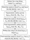 |
Fig. 2 Schematic overview of iterative spectro-trigonometric analysis. Boxes represent individual analysis steps, with updated parameters listed below the horizontal line. Arrows indicate the workflow from top to bottom. Effective temperatures and initial surface gravities were constrained from Balmer line wings, trigonometric surface gravities were derived from stellar mass, bolometric magnitude, and temperature, and metal lines were used to refine all remaining atmospheric parameters until convergence was achieved. |
3.2 Spectral analysis
This section builds on the differences outlined above and details the complete analysis procedure applied to the hot star sample. We derived stellar parameters using the ZEEMAN spectral synthesis code (Landstreet 1988; Wade et al. 2001; Folsom et al. 2012), which calculates LTE synthetic spectra and fits them to observed spectra using a χ2 minimisation algorithm (Folsom et al. 2012). We used the latest version (20 Apr 2025) of ZEEMAN, which incorporates several improvements, detailed here. The Balmer line calculation is described in Folsom et al. (2022). Hyperfine splitting and isotopic splitting are supported through the calculations in VALD (Pakhomov et al. 2019), which can return these components as separate lines. More advanced van der Waals broadening coefficients, calculated using the theory of Anstee & O’Mara (1995) and Barklem & O’Mara (1997) were used if available. Improvements to Stark broadening profiles for some He lines were described by Folsom et al. (2022) (using Barnard et al. 1969, 1974, 1975), which have been supplemented with the Stark broadening tables for He of Dimitrijevic & Sahal-Brechot (1990). Continuous opacities were extended to include bound-free and free-free opacity from the H and He
 from Stancil (1994) (in addition to existing opacities from H, H−, He I, He II, and electron scattering). Partition functions approximations from Irwin (1981) were used.
3.2.1 Line lists and oscillator strength corrections
As described in Sect. 3.1, we created a merged line list with log gf corrections suitable for both benchmark and hot stars. A full description of the line list merging and log gf corrections is provided in Appendix A. High-quality lines (flagged as ‘Y’) in the original Gaia-ESO list were included. Lines with an undecided quality (flagged as ‘U’) were compared with lines from VALD, using observations of standard stars (Sun (G2V), Pro-cyon (F5IV-V), and 21 Peg (B9.5V)) and synthetic spectra, and the data that better reproduced the observations were retained. Lines flagged as not recommended (‘N’) were rejected. Lines forming their ‘background line list’, (from VALD version 820, in Sept 2014) were replaced by updated entries from VALD.
The log gf corrections were applied to all hyperfine or isotropic components of each line, resulting in 2750 corrections for the full list of 26 665 lines available on Zenodo3. These empirical oscillator-strength corrections were applied to approximately 10% of transitions only when high-quality atomic data were unavailable. No recommended ‘Y’ lines from the Gaia-ESO or reliable NIST values were modified.
3.2.2 Normalisation
Before the fitting procedure, all spectra were continuum-normalised using a custom Python tool that fits low-order polynomials to individual echelle orders (Folsom et al. 2025)4. Since the original echelle order boundaries were not available for most spectra, and because the majority of hot-star spectra exhibit relatively smooth continua, we divided the spectra into uniform 100 Å segments for polynomial normalisation. This approach is robust and computationally efficient for smooth continua. For spectra with more complex continuum shapes (e.g. ESPRESSO spectra), the SUPPNET python code was used (Różański et al. 2022)5. Balmer lines were normalised using a different approach (see below).
3.2.3 Balmer line analysis
Balmer lines provided initial estimates of Teff and log g for all stars, and independent Teff values in the final result. For A-type and early F-type stars, Balmer line wings are sensitive to temperature, with only a weak dependence on surface gravity (e.g. Gray 2008), and are relatively insensitive to other parameters such as metallicity, microturbulent velocity, and projected rotational velocity. This makes them valuable as an independent constraint, especially for hot, rapidly rotating stars where metal lines are sparse or blended. In order to minimise the impact of non-LTE effects in the line cores, we removed them. We simultaneously fitted the continuum, Teff , and log g to the unnormalised spectrum around each Balmer line, while modelling the local continuum with a second-degree polynomial. As continuum placement and Teff are not strictly independent, we tested the approach on standard stars and verified that it yields consistent effective temperatures and reliable initial log g. We fitted individual lines from Hα to Hδ, when available, and used their average value. The reported uncertainties are from the standard deviation across the independently fitted Balmer lines for each star. Examples of Balmer line fits are shown in Figure B.3.
3.2.4 Metal-line analysis
After the initial guess of Teff and log g, we obtained other parameters using spectral fitting. Each spectrum was divided into multiple windows for independent analysis. To ensure internal consistency, we kept the windows roughly the same for all hot stars. While the choice of window boundaries does not significantly affect the final atmospheric parameters, it does influence the associated uncertainties. Due to severe line blending in the spectra of hot stars, we used four windows, edges depending on the star, each spanning ≈300-470 Å. In contrast, the cooler benchmark stars exhibit denser spectral features, so we decided to use narrower windows of approximately 200 Å. Within each window, the atmospheric parameters were fitted simultaneously following the scheme described in Sect. 3 and illustrated in Fig. 2. Depending on the iteration step, Teff was either held fixed or allowed to vary together with [Fe/H], [M/H], v sin i, and vmic. When required, the local continuum was re-fitted using Chebyshev polynomials to account for normalisation imperfections. Initial parameter inputs required for the model atmosphere calculations (namely Teff, log g, ν sin i) were adopted from the Ariel MCS list when available. The initial microturbulent velocity, vmic, was estimated as described in 3.2.6, and the solar metal-licity was adopted as an initial guess for the metallicity. These values serve only as starting points for the spectral fitting. For all hot stars, Balmer-line fits provided final effective temperatures. We averaged results across all windows to determine final parameters, adopting the standard deviation as the uncertainty to reflect consistency across windows. The final parameters are provided in Table 2.
3.2.5 NLTE effects
Departures from local thermal equilibrium (LTE) primarily affect Fe I lines in A-F-type stars through over-ionisation. Mashonkina (2011) reported non-LTE corrections of 0.02-0.10dex for FeI and <0.03 dex for FeII, with the magnitude of the effect decreasing towards higher effective temperatures. Since our analysis relies mainly on the wings of the Balmer lines to derive Teff and on trigonometric log g, such non-LTE effects are not expected to significantly influence our final stellar parameters.
3.2.6 Micro-and macroturbulence velocity
For stars with Teff < 6500 K, the initial values of vmic were estimated using the empirical relation from Tsantaki et al. (2013):
 (1)
(1)
For hotter stars, initial values were adopted from Gebran et al. (2014), with typical uncertainties of 25%, and further refined during spectral fitting.
Macroturbulence velocity (vmac) was treated differently for hot and cool stars. For benchmark stars, we adopted empirical relations from Doyle et al. (2014), consistent with T25. These are valid for dwarfs with 5200K < Teff < 6400K and log g > 4.0. Similar to T25, for benchmark stars falling out of these ranges, we followed Valenti & Fischer (2005).
For the hot star sample, the macroturbulence velocity was set to zero, as rotational broadening dominates line profiles in this regime. Although some studies (e.g. Doyle et al. 2013; Psaridi et al. 2023) extrapolate macroturbulence from Gray (2008) up to ∼6700K, these relations remain uncertain, particularly for A-type stars. We note that setting vmac = 0 may lead to a mild overestimation of v sin i, especially with host stars with low ν sin i such as WASP-178, but the value remains within error margins and does not affect the determination of other stellar parameters.
Fundamental parameters of hot stars derived in this work.
3.2.7 Trigonometric surface gravity
Similarly to M22 and T25, surface gravity was obtained using the following relation:
 (2)
(2)
where M* is the stellar mass in solar mass units, Mbol is the bolometric magnitude, Teff is the effective temperature adopted at each iteration (initially from Balmer-line fitting and updated during the iterative analysis), and 12.505 is a normalisation factor to the solar surface gravity. The bolometric magnitude, Mbol (and consequently the luminosity), was derived by a Markov chain Monte Carlo (MCMC)-based fitting procedure, which takes input as a combination of several magnitudes and the distance. This procedure does not perform a spectral energy distribution (SED) fit; instead, the MCMC sampler predicts theoretical magnitudes from bolometric corrections and compares them to the observed photometry. The magnitudes considered are taken from 2MASS (J, H, and Ks bands; Skrutskie et al. 2006), Gaia (GBP and GRP; Gaia Collaboration 2021), and, when available, Johnson B and V magnitudes. The Johnson magnitudes are taken from the synthetic photometry generated from Gaia BP/RP mean spectra (Gaia Collaboration 2023). Each magnitude was converted to bolometric magnitude using YBC bolometric correction library (Chen et al. 2019), which interpolates a series of precomputed tables of bolometric correction in Teff, [Fe/H], log g and extinction, AV. In this specific step, log gtrig was used only to determine the bolometric corrections and was not treated as an evolutionary constraint. The distance was derived by a simple parallax inversion, with the parallax given by Gaia EDR3. The masses were derived using the Bayesian tool PARAM (da Silva et al. 2006; Rodrigues et al. 2014, 2017), which performs isochrone fitting by comparing observed parameters (such as metallicity, effective temperature, and photometric luminosity) with a grid of theoretical stellar models (Moedas et al. 2022). Importantly, log gtrig was not fitted to the evolutionary tracks, but was derived independently from the resulting mass, luminosity, and temperature using Equation (2). The metal-line fitting was repeated with log g fixed to the trigonometric value, iterating until the parameters converged. All fits were inspected visually. In Figure B.1, we show the observed, model, and difference spectra for the hot stars.
3.3 Peculiar stars
Several stars in our sample are known chemically peculiar stars: HATS-70, KELT-17, TOI-1431, and WASP-178. Literature reports for these targets indicate either strong or weak Am-type abundances (underabundant Ca and Sc and overabundant iron-peak elements). For these stars, our standard fitting procedure was applied to determine the overall metallicity [M/H] and iron abundance [Fe/H]. However, given the peculiar abundance patterns in such stars, the derived parameters should be interpreted with caution. Am-type chemical peculiarity is generally associated with slow rotation in stars hotter than approximately 7000 K. In our analysis, we notice a >0.1 dex difference between [Fe/H] and [M/H] for these known peculiar stars (see Table 2). We adopted this offset as a preliminary diagnostic flag for potential peculiarity in other targets. Specifically, stars with lower ν sin i such as HD-2685, TOI-615, WASP-172, and potentially KOI-13 and TOI-1518 fall within the regime where diffusion-driven abundance anomalies may occur. In addition, WASP-189 was classified as non-Am by Saffe et al. (2021) and Anderson et al. (2018), whereas Lendl et al. (2020) reported Am-type peculiarities for this star. A definitive Am classification requires a full spectral classification analysis (e.g. using MK classification methods6) or detailed element-by-element abundance studies, both of which are beyond the scope of this work. These analyses will be performed in future work and may lead to further refinements of fundamental parameters such as Teff and possibly log g.
3.4 Consistency with previous works
To assess the consistency of our methodology, we analysed a set of 23 benchmark stars, previously studied in M22 and T25, using the methodology described in Sect. 3.2. Figure 3 compares our inferred stellar parameters (Teff, log g, [Fe/H], ν sin i, and νmic) with those from M22 and T25 (hereafter ‘previous work’), showing normalised residuals relative to the previous estimates (left panels) and their distributions (right panels). We present the residuals with respect to M22 and T25 separately, as their methodologies, though equivalent, are not identical (see T25 for details). For the benchmark stars, we derived effective temperatures using both Balmer-line and metal-line diagnostics to assess which method is more reliable in different temperature regimes. A comparison with M22 and T25 reveals an empirical transition at Teff≃6600 K. Below this temperature, Balmer-line fits systematically overestimate effective temperatures due to increased metal-line blending in the wings. However, above this threshold, Balmer-line and metal-line diagnostics converge, showing excellent agreement (e.g. 0 K difference for HAT-P-2). This transition point guides our methodology: we adopted Balmer-line temperatures for the hot-star sample to ensure an internally consistent scale that maintains continuity with the cooler stars analysed in previous works. Table B.2 provides the effective temperatures derived from metal-line analysis (Teff) and from Balmer-line fits (Teff,Balmer) for all benchmark stars, allowing for a direct comparison between the two diagnostics.
Outliers exist in Teff, log g, or [Fe/H] panels, with normalised residuals lying outside the 3σ level. The largest scatter among the remaining parameters is seen for νmic, which displays several points that are clearly inconsistent at the >3σ level, suggesting that its uncertainties may be underestimated. This increased scatter in υmic is expected in cross-study comparisons. Microturbulent velocity is not a directly observable quantity and is treated differently in previous works, being either fitted, constrained, or computed from empirical relations (see Sect. 3.2.6). In contrast, ν sin i values appear fairly consistent between the two analyses, although with a small median offset. The uncertainties in ν sin i naturally increase with the rotation rate, illustrating the challenges of analysing rapid rotators. FASMA performs well for stars up to ν sin i ~50 km/s, while ZEEMAN is used to analyse stars with even higher projected rotational velocities. The stars flagged as outliers are HR 858, KELT-2A, TOI-677, K2-99, and WASP-166 (orange points in Fig. 3), whose normalised residuals in Teff exceed 3σ. These stars also show systematically higher inferred values of log g and [Fe/H], and all five stars seem to have underestimated uncertainties. For Teff, our average uncertainties are 36 K (38 K in T25). For log g and [Fe/H] 0.03 (0.01 dex T25) dex and 0.04 (0.03 dex T25) dex, respectively. We also assessed how residuals in Teff, log g, and [Fe/H] vary as a function of the M22 and T25 values (Fig. B.2). No significant correlations are found, although a weak tendency for higher Teff values at lower metallicities is visible (r = −0.40, p = 0.06). T25 similarly reported a ∼145 K Teff overestimation compared to M22 for stars with [Fe/H] < − 0.25 dex, without significant offsets in log g or [Fe/H]. These results suggest that small residual trends may originate from the interplay between Teff and [Fe/H], while log g remains largely unaffected.
The coolest target in our benchmark set, V1298 Tau, is a premain-sequence star published in M25 (marked in Fig. 1 and also in Fig. 3 in red). However, given that the isochrone grids used for stellar mass estimation were not calibrated for young stars, it has now been excluded from the Ariel Stellar Catalogue.
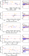 |
Fig. 3 Left panels : normalised residuals defined as the difference between this work’s estimates and previous ones, divided by the propagated uncertainty of both estimates plotted against previous estimates from M22 and T25. Outliers are defined as stars with normalised residuals lying outside the 3σ region, marked by the dashed red lines. Orange points indicate the 5 stars from T25 for which Teff is above 3σ. Median and median absolute deviation (MAD) values are indicated in each panel. Right panels : distribution of normalised residuals. The red curve shows a standard normal distribution (mean zero, variance one) to ease visual assessment of consistency between works. |
4 Results
Here we present our results for the sample of hot stars in the MCS. The final sample comprises 18 stars with spectral types from late F to early A. Consistency checks on the benchmark sample (Sect. 3.4) show that our methodology yields results broadly consistent with those in T25 and M22. Small offsets and trends in Teff and [Fe/H] were mitigated by adopting Teff values from Balmer-line fitting for the final metallicity analysis. With these offsets characterised, our results are placed on the same scale as the cooler-star analyses in M22 and T25, enabling a consistent comparison of stellar parameters across a wide temperature range for the Ariel MCS.
4.1 Overview of hot star parameters
The Kiel diagram (Fig. 1) shows the hot star sample alongside the cooler stars from previous works, overlaid with PARSEC isochrones7 of solar and super-solar metallicity. The new targets occupy the upper main sequence above ∼6900 K. All parameters and uncertainties are listed in Table 2. Combined with the cooler FGK stars analysed in M22 and T25, the total number of Ariel MCS stars with internally consistent parameter determinations now stands at 370.
Figure 4 shows the distributions of Teff, log g, [Fe/H], and stellar mass and the projected rotational velocities for the hot star sample (shown in red) compared with the M22 and T25 sample (shown in blue). Our sample is concentrated at M* > 1.4 M⊙ and extends up to ∼2.3 M⊙, substantially expanding the high-mass tail of the Ariel MCS. The metallicity range is similar to that of the cooler star sample, dominated by solar and supersolar values.
Figure 5 shows the microturbulent velocity as a function of Teff. The trend follows well-known temperature dependence of microturbulence in A-F stars: vmic rises from late-F to early-A types, reaching a maximum around Teff ∼ 8000 K, and then decreases towards hotter stars (e.g. Landstreet et al. 2009). Figure 6 shows v sin i as a function of stellar mass, colour-coded by Teff. The relation between v sin i and stellar mass follows the expected trend: the rotation rates are higher at larger masses. The fastest rotators are KELT-21, KELT-20, KELT-9, and MASCARA-1, which span masses from ∼1.6 to 2.3 M⊙ and effective temperatures from ∼8000 to ∼9400 K. In contrast, TOI-1431 is among the slowest rotators in the sample with v sin i ~ 8 kms−1. The hottest stars in the sample (Teff ≳ 8000 K) tend to rotate the fastest, consistent with their thinner convective envelopes and weaker magnetic braking. At a given mass, however, there is significant scatter, with some intermediatemass stars showing relatively slow rotation (v sin i ≲ 40 kms−1). Most of these slow rotators also exhibit chemical peculiarities, as mentioned in Section 3.3.
4.2 Kinematic properties
Figure B.6 shows the kinematic properties of the hot star sample compared to the T25 sample in the Toomre diagram (left) and the Galactic orbital parameter space (right). All hot stars lie within the thin disc region (|Vtot| < 50 km s−1), consistent with a young, local population. Their orbital parameters indicate they are located near the solar Galactocentric radius (RGC ~ 8 kpc) with minimal radial excursions, suggesting they have not migrated significantly from their birthplaces. This is expected for massive, short-lived main-sequence stars, which do not survive long enough to experience substantial radial migration.
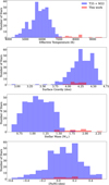 |
Fig. 4 Distributions of homogeneously derived stellar parameters for the Ariel mission candidate sample. The red histograms represent the stars analysed in this work, while the filled blue bins show results from our previous analysis (T25 and M22). |
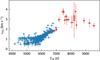 |
Fig. 5 Microturbulent velocity as a function of Teff. Red points are stars from this analysis and blue points are stars from M22 and T25. |
 |
Fig. 6 Projected rotational velocity (v sin i) as a function of stellar mass, colour-coded by effective temperature. Hot fast rotators analysed in this work are highlighted with a black circle. |
4.3 Comparison of hot star parameters with literature values
We compared our derived stellar parameters with those available in the literature. In particular, we focused on the works of Saffe et al. (2021, 2022), who have conducted detailed analyses of early-type stars, including both atmospheric parameters and chemical abundances. Similar to us, they employed high-resolution spectroscopy and synthetic spectrum fitting techniques to derive atmospheric parameters.
We validated our results against literature values using normalised residuals (Fig. 7). Each panel shows the residuals divided by propagated uncertainties as a function of the literature value, with the median and MAD annotated. The majority of stars cluster around zero residuals, confirming consistency with previous works within the quoted uncertainties. A few >3σ outliers are seen: KELT-21 in Teff and [Fe/H], and HAT-P-57 and KELT-17 in ν sin i.
The literature values for KELT-21 are taken from Johnson et al. (2018), who used the Payne algorithm (see references therein) to model individual TRES spectra by fitting a ∼200 Å region around the Mg I triplet near 5200 Å. Since we used Balmer line analysis as an independent method of determining Teff together with independent log g estimation, our values are expected to be more robust. Our Teff is closer to the value Johnson et al. (2018) derived using SED and in better agreement with the Gaia DR3 parameters. Specifically, Gaia DR3 reports Teff =  K and [Fe/H] =
  dex, whereas Johnson et al. (2018) derived Teff =
  K and [Fe/H] =
  dex. Such a low [Fe/H] is unlikely for an early A-type thin-disc star and may result from limitations of automated approaches such as the Payne. The results can be affected by high rotational broadening, which reduces sensitivity to metallicity diagnostics and biases fits towards lower values. As for HAT-P-57 (94 ± 1.7 km s−1 versus 102 ± 1.3 in Hartman et al. (2015) and KELT-17 (46.2 ± 0.5 km s−1 versus 43.0 ± 0.6 in Saffe et al. (2021), the outliers in ν sin i arise from underestimated formal uncertainties rather than real discrepancies.
5 Discussion
Our results extend the known parameter space of stellar hosts towards the high-temperature range, providing the first consistent analysis of A-type planet hosts within the Ariel sample. Hot stars are particularly relevant for exoplanet studies, as their relatively line-poor spectra make them favourable targets for transmission and emission spectroscopy. Moreover, giant planets around A-type stars are intrinsically rare (Borgniet et al. 2019), meaning each system provides a valuable probe of planet formation and migration around intermediate-mass stars. This new subsample therefore fills an important gap in the Ariel stellar characterisation, linking the hotter end of the main sequence to the cooler FGK hosts analysed in M22 and T25.
In this section, we extend the study of planet-star connections presented in our previous works. We use planetary parameters from the NASA Exoplanet Archive8. The characteristics of the planet and hot host star systems can be found in Table B.1.
 |
Fig. 7 Left panels : same as in Fig. 3, but for 18 hot stars. Literature values are from Hartman et al. (2015); Zhou et al. (2019b); Jones et al. (2019); Niemczura et al. (2017); Johnson et al. (2018); Kama et al. (2023); Addison et al. (2021); Cabot et al. (2021); Hellier et al. (2019b,a); Lendl et al. (2020); Psaridi et al. (2023); Saffe et al. (2021), and Saffe et al. (2022). Right panels : distribution of normalised residuals. The red curve shows a standard normal distribution (mean zero, variance one). |
5.1 Stellar metallicity and exoplanet populations
T25 confirmed that stellar metallicity influences planet populations, using a mass threshold of Mp = 0.2 MJ to distinguish between low- and high-mass systems. Their results showed that low-mass planets preferentially orbit metal-poor stars, while high-mass planets typically orbit metal-rich hosts.
All 18 hot stars analysed in this work host hot Jupiters, and therefore fall into the massive-planet category. The inclusion of this new subsample keeps the overall median of the metallicity distribution around 0.1 dex (Fig. 8).
Furthermore, in Sect. 4.2 we showed that all of our hot stars belong to the thin disc. This is expected, as intermediate-mass A-F stars are relatively young. Their youth and Galactic disc inheritance makes them enriched in heavy elements, providing more building blocks for giant planet formation. For a broader discussion of the implications for thin- and thick-disc stars, we refer to T25. Future detailed abundance analyses of our hot sample will provide a more robust test of Galactic membership.
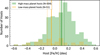 |
Fig. 8 Host star metallicity distributions for Ariel target candidate sample systems with low-mass planets (Mp < 0.2 MJ; yellow) and high-mass planets (Mp ≥ 0.2MJ; green). Solid vertical lines mark the median [Fe/H] values, and the dotted lines indicate the 95% confidence intervals. |
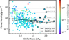 |
Fig. 9 Planet density as a function of stellar mass. The points are colour-coded by semi-major axis (AU), with a logarithmic colour scale. Solid and dashed black lines show linear fits for high- and low-metallicity hosts ([Fe/H] ≥ 0 and < 0, respectively), considering only planets more massive than 0.2 MJ. Following the compositional density divisions from Zeng et al. (2019), we indicate reference lines at ρ ~ 1, 3.3, and 8 g cm−3 corresponding respectively to a water- or ice-rich, silicate-rocky, and iron-rich bulk composition. Black circles highlight the 18 stars analysed in this work. |
5.2 Dependence of planetary structure on stellar mass and metallicity
To capture the combined effects of stellar mass and metallicity, we examined the relation between planetary density and stellar mass (Fig. 9). Planet density decreases towards higher stellar masses, consistent with the enhanced radius inflation expected for planets orbiting more luminous A-F-type hosts. We still observe a significant scatter among planets around intermediatemass stars, which is partly explained by uncertainties in planetary masses; six planets in our hot sample have only upper limits on their masses, which artificially raises their inferred densities and flattens the overall planet-density-stellar-mass trend.
At a given stellar mass, planets around metal-rich stars are systematically denser, indicating a larger heavy-element fraction or more massive cores, in agreement with the metallicity-density trend reported by Biazzo et al. (2022). Together, these results support a picture in which metallicity regulates the internal heavy-element content, while stellar mass primarily drives envelope expansion through irradiation.
To isolate the physical mechanism behind this trend, we examined planetary density as a function of intercepted stellar power (Fig. B.5). A strong anti-correlation is observed for giant planets: systems receiving higher incident power host less dense planets, demonstrating that irradiation is the dominant driver of radius inflation. Inflation becomes significant once the incident flux exceeds approximately 2 × 10⁸ erg s−1 cm−2 (or equivalently ∼2 × 10⁵ W m−2), the empirical threshold at which hot-Jupiter radii begin to rise sharply (e.g. Demory & Seager 2011). Most planets in our hot-star sample lie well above this threshold, consistent with their large radii.
At fixed incident power, giant planets around metal-rich stars remain denser, reinforcing the role of metallicity in setting bulk composition. These results extend the trends previously identified for FGK hosts in T25 to the higher-mass A-F stars analysed in this work. Following T25, we examined radius-stellar mass correlation separately (Appendix B.4). This is consistent with a scenario where both stellar luminosity and mass both drive planetary radius inflation.
5.3 Multi-planet systems and their relation with the stellar mass, metallicity, and total planetary mass
We computed the total planetary mass for the subsample of multi-planetary systems, using measured values where available and lower limits otherwise, to assess its dependence on stellar mass and metallicity (Fig. B.7). Our results indicate a clear positive correlation between total planetary mass and stellar mass across the parameter space considered. This finding is consistent with the established relationship between stellar mass and the dust and gas masses of protoplanetary discs (Pascucci et al. 2016; Testi et al. 2022), suggesting that the initial disc mass budget is a primary factor in setting the ultimate planetary system mass consistently with the results of population synthesis studies (e.g. Savvidou & Bitsch 2023; Burn & Mordasini 2024). Upon dividing the sample by metallicity, a strong positive trend is evident for solar (−0.2 < [Fe/H] < 0.2) and super-solar stars ([Fe/H] > 0.2). We attribute this enhanced planetary mass growth to the greater abundance of solid materials in the protoplane-tary discs allowed by the larger metallicity (e.g. Filomeno et al. 2024). In such metal-rich environments, planetary core accretion proceeds efficiently, leading to an earlier onset of runaway gas accretion while the disc is still massive and capable of supplying substantial gaseous material to the growing planet. In contrast, the sub-solar bin shows a flat trend, with total masses below the threshold of giant planets (i.e., 0.2 MJ as defined in Magrini et al. 2022; Tsantaki et al. 2025). In these metal-poor systems, slower core formation delays the onset of gas accretion until the disc is depleted (e.g. Savvidou & Bitsch 2023; Filomeno et al. 2024), limiting growth and promoting the formation of multiple, similarly sized planets rather than a single dominant one.
To probe the intra-system mass distribution of the planetary systems, we adopted the metric ML = Mp/Mtot (Chambers 2001) that we expressed as the percentage [%] of the total planetary mass, Mtot, contained in the most massive planet in the system (of mass MP). This allowed us to analyse the architectural trends as a function of the stellar mass. In Fig. 10 we see that, in the same Mtot range of the systems around stars with subsolar metallicity discussed above (see also Fig. B.7), the most massive planet typically contains 25-75% of the total planetary mass, a range encompassing systems with relatively similar planets to systems with a mass concentration comparable to that of the Solar System (ML,Jupiter ≈ 0.7). Systems with a higher mass concentration (ML > 75%) exclusively have a multiplicity of N = 2 and are among the most massive systems in the sample (the majority is above Mtot > 0.2 MJ) This suggests that, for high-mass systems, either dynamical instability or efficient accretion by a single body shaped their final architecture. Conversely, systems with a lower mass concentration (ML < 50%) are characterised by N > 2. All of them have Mtot < 0.2MJ, and show an opposite trend, with Mtot decreasing with the stellar mass.
To further investigate these behaviours, we divided the sample into three total-mass bins: low-mass systems (Mtot < 0.2 MJ), mid-mass systems (0.2 < Mtot < 10 MJ), and high-mass systems (Mtot > 10 MJ). High-mass systems predominantly have N = 2 (Fig. 11, left). This suggests either the formation of fewer, massive planets, or a later dynamical evolution via planet-planet scattering, which can create a dominant body through collisions or ejections (Zinzi & Turrini 2017; Turrini et al. 2020). Mid-mass systems show a binomial multiplicity distribution (peaks at N=2 and N=4), while low-mass systems span a wider range (N up to 6), consistent with Kepler’s ‘peas-in-a-pod’ pattern (Weiss et al. 2018).
To probe their dynamical histories, we analysed the eccentricity of the largest planet in each system (Fig. 11, right). High-mass systems are dominated by planets with e > 0.5, strongly indicating a chaotic, scattering-driven evolution history (Zinzi & Turrini 2017; Turrini et al. 2022). Mid-mass systems have a binomial eccentricity distribution split near e = 0.1, likely separating dynamically evolved from primordial systems. Low-mass systems show a more continuous eccentricity distribution, suggesting only moderate instabilities occurred, as weaker mutual perturbations are less likely to be catastrophic (Turrini et al. 2020, 2022).
Finally, we examined the orbital separation of the largest planets (Fig. 12). For low-mass systems, the semi-major axis shows little scatter. In contrast, the dispersion increases dramatically for mid- and high-mass systems, with the most massive planets spanning a wide range of orbital distances (0.02-3 AU). This broad distribution further supports once again a history of chaotic evolution for the most massive planetary systems resulting in wider orbital architectures (Rasio & Ford 1996; Weidenschilling & Marzari 1996).
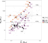 |
Fig. 10 Total planetary mass available in each planetary system, as a function of the stellar mass (with error bars), colour-coded by the ML metric (see main text). The grey dots represents the mass of planets in single planet systems. Dashed lines are plotted to provide a visual range of masses in terms of MJ. The black cross identifies the Solar System and stellar mass errors are reported for each system. |
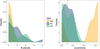 |
Fig. 11 Multiplicity distribution (left panel) and distribution of the eccentricity of each largest body in the system (right panel). Each distribution is colour-coded based on the total mass bins: low-mass, mid-mass, and high-mass (see text for more details). Dashed line marks the eccentricity value of e = 0.1 (see text for more details). |
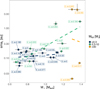 |
Fig. 12 Semi-major axis of the largest body in the system, as a function of the host stellar mass, and colour-coded by the total mass in each system. The dashed regression lines are plotted for trend identification purposes. Labels indicate the multiplicity, N, and the eccentricity for each planet. Stellar mass and semi-major axis errors are reported for each system. |
6 Conclusions
We have presented analysis of 18 high-temperature (Teff > 6800 K) stars in the Ariel candidate sample using an internally consistent methodology optimised for hot, rapidly rotating stars. The results complement the FGK host-star studies of Magrini et al. (2022) and Tsantaki et al. (2025), extending the stellar parameter space towards earlier spectral types.
Stellar parameters: we derived fundamental parameters (Teff, log g, mass, [Fe/H], [M/H], νmic, and v sin i, ) for 18 stars using an iterative spectro-trigonometric method tailored for hot and fast-rotating stars. The approach incorporates updated line lists, empirical oscillator-strength corrections, Balmer-line constraints, and large wavelength windows suitable for rapid rotators. A comparison with 23 benchmark stars shows good overall agreement with previous Ariel analyses, ensuring that our results are internally consistent and placed on a comparable scale with the cooler-star studies in the Ariel MCS.
Chemically peculiar stars: several targets exhibit properties providing a preliminary indication of possible Am-type chemical peculiarity. A subset of the sample (HATS-70, KELT-17, TOI-1431, and WASP-178) has already been identified as chemically peculiar in previous studies, while for the remaining stars the indications are based on rotational properties and global metallicity trends. However, a detailed element-by-element abundance analysis is required to confirm the presence and degree of chemical peculiarity for the full sample, and will be carried out in future work.
Kinematics: the entire hot-star sample is consistent with thin-disc kinematics, in line with their relatively young ages and near-solar metallicities.
Planet-star correlations: the trends previously observed for FGK hosts also persist for hotter stars. Giant-planet radii increase toward higher stellar masses, primarily reflecting stronger stellar irradiation, while remaining metallicity dependent: at a given stellar mass, planets around metal-poor hosts tend to have larger radii, while planets around metalrich hosts are generally more compact, consistent with differences in heavy-element content. The density-stellar-mass plane shows the same qualitative behaviour, although with additional scatter caused in part by heterogeneous planetary parameters and mass upper limits, which can artificially affect the inferred densities.
Overall, our results indicate that the star-planet correlations identified for FGK hosts also extend to more massive, early-type stars. These findings highlight the importance of including high-temperature stars when assessing the diversity of planets and refining the target selection for the Ariel mission. Furthermore, they highlight how stellar properties shape the global architecture of multi-planet systems and the path of their dynamical evolution, imprinting on their multiplicity, mass and mass distribution, and dynamical excitation.
Data availability
All parameters presented here (Table 2) are available via the Ariel Stellar Catalogue: https://bit.ly/ArielStellarCatalogue. The latter also includes atmospheric parameters ([Fe/H], Teff, log g, νmic, ν sin i), kinematic properties and C, N, O abundances for the cooler sample of planet-host FGK dwarf stars.
Acknowledgements
This work has been developed within the framework of the Ariel “Stellar Characterisation” and “Planet Formation” working groups of the ESA Ariel space mission Consortium. H.R., S.B., C.P.F., A.L., V.M. and M.K. acknowledge funding from the European Union’s Horizon Europe research and innovation programme under grant agreement No. 101079231 (EXOHOST) and from UK Research and Innovation (UKRI) under the UK government’s Horizon Europe funding guarantee (grant number 10051045). The research was conducted using the ESA Estonia research infrastructure funded by the Estonian Research Council grant TARISTU24-TK3. This work has made use of the VALD database, operated at Uppsala University, the Institute of Astronomy RAS in Moscow, and the University of Vienna; the VizieR catalogue access tool CDS, Strasbourg, France (DOI : 10.26093/cds/vizier). C.D. acknowledges financial support from the grant RYC2023-044903-I, funded by MCIU/AEI/10.13039/501100011033 and by the ESF+, and from the INAF initiative “IAF Astronomy Fellowships in Italy”, grant name GExoLife. D.T. acknowledges support from the Italian Space Agency (ASI) through the ASI-INAF grant no. 2021-5-HH.0 plus addenda no. 2021-5-HH.1-2022 and 2021-5-HH.2-2024, the COST Action CA22133 PLANETS, and the European Research Council via the Horizon 2020 Framework Programme ERC Synergy “ECOGAL” Project (project ID GA-855130). D.B. acknowledges funding support by the Italian Ministerial Grant PRIN 2022, “Radiative opacities for astrophysical applications”, no. 2022NEXMP8, CUP C53D23001220006. L.M. thank INAF for the support (Large Grants EPOCH and WST), the Mini-Grants Checs (1.05.23.04.02), and the financial support under the National Recovery and Resilience Plan (NRRP), Mission 4, Component 2, Investment 1.1, Call for tender No. 104 published on 2.2.2022 by the Italian Ministry of University and Research (MUR), funded by the European Union - NextGenerationEU - Project ‘Cosmic POT’ Grant Assignment Decree No. 2022X4TM3H by the Italian Ministry of the University and Research (MUR). K.G.H. acknowledges support from NCN grant 2023/49/B/ST9/01671. H.R. thanks Luca Fossati, Anish Amarsi, and Indrek Kolka for their support and insightful comments. The team is very grateful to the service astronomers who performed our observations at ESO TNG (with HARPS-N during A41, A46). Based on observations collected at the European Southern Observatory under ESO programmes and with the SOPHIE spectrograph on the 1.93 m telescope at the Observatoire de Haute-Provence (CNRS), France, by the SOPHIE RPE Consortium (program PNP.CONS).
References
- Addison, B. C., Knudstrup, E., Wong, I., et al. 2021, AJ, 162, 292 [NASA ADS] [CrossRef] [Google Scholar]
- Adibekyan, V., Santos, N. C., Figueira, P., et al. 2015, A&A, 581, L2 [NASA ADS] [CrossRef] [EDP Sciences] [Google Scholar]
- Adibekyan, V., Dorn, C., Sousa, S. G., et al. 2021, Science, 374, 330 [NASA ADS] [CrossRef] [Google Scholar]
- Anderson, D. R., Temple, L. Y., Nielsen, L. D., et al. 2018, MNRAS submitted [arXiv:1809.04897] [Google Scholar]
- Anstee, S. D., & O’Mara, B. J. 1995, MNRAS, 276, 859 [Google Scholar]
- Barklem, P. S., & O’Mara, B. J. 1997, MNRAS, 290, 102 [Google Scholar]
- Barnard, A. J., Cooper, J., & Shamey, L. J. 1969, A&A, 1, 28 [NASA ADS] [Google Scholar]
- Barnard, A. J., Cooper, J., & Smith, E. W. 1974, J. Quant. Spec. Radiat. Transf., 14, 1025 [NASA ADS] [CrossRef] [Google Scholar]
- Barnard, A. J., Cooper, J., & Smith, E. W. 1975, J. Quant. Spec. Radiat. Transf., 15, 429 [Google Scholar]
- Barnes, J. W., Linscott, E., & Shporer, A. 2011, ApJS, 197, 10 [NASA ADS] [CrossRef] [Google Scholar]
- Biazzo, K., D’Orazi, V., Desidera, S., et al. 2022, A&A, 664, A161 [NASA ADS] [CrossRef] [EDP Sciences] [Google Scholar]
- Borgniet, S., Lagrange, A.-M., Meunier, N., et al. 2019, A&A, 621, A87 [NASA ADS] [CrossRef] [EDP Sciences] [Google Scholar]
- Borsa, F., Rainer, M., Bonomo, A. S., et al. 2019, A&A, 631, A34 [NASA ADS] [CrossRef] [EDP Sciences] [Google Scholar]
- Buchhave, L. A., Bizzarro, M., Latham, D. W., et al. 2014, Nature, 509, 593 [Google Scholar]
- Burn, R., & Mordasini, C. 2024, in Handbook of Exoplanets, 143-2 [Google Scholar]
- Cabot, S. H. C., Bello-Arufe, A., Mendonça, J. M., et al. 2021, AJ, 162, 218 [NASA ADS] [CrossRef] [Google Scholar]
- Castelli, F., & Kurucz, R. L. 2003, in Modelling of Stellar Atmospheres, 210, eds. N. Piskunov, W. W. Weiss, & D. F. Gray, A20 [NASA ADS] [Google Scholar]
- Chakrabarty, A., & Sengupta, S. 2019, AJ, 158, 39 [NASA ADS] [CrossRef] [Google Scholar]
- Chambers, J. E. 2001, Icarus, 152, 205 [Google Scholar]
- Chen, Y., Girardi, L., Fu, X., et al. 2019, A&A, 632, A105 [EDP Sciences] [Google Scholar]
- Collier Cameron, A., Guenther, E., Smalley, B., et al. 2010, MNRAS, 407, 507 [NASA ADS] [CrossRef] [Google Scholar]
- Cowan, N. B., & Coull-Neveu, B. 2025, OJAp, 8, E160 [Google Scholar]
- da Silva, L., Girardi, L., Pasquini, L., et al. 2006, A&A, 458, 609 [NASA ADS] [CrossRef] [EDP Sciences] [Google Scholar]
- da Silva, R., Danielski, C., Delgado Mena, E., et al. 2024, A&A, 688, A193 [NASA ADS] [CrossRef] [EDP Sciences] [Google Scholar]
- Danielski, C., Brucalassi, A., Benatti, S., et al. 2022, Exp. Astron., 53, 473 [NASA ADS] [CrossRef] [Google Scholar]
- de Laverny, P., Ligi, R., Crida, A., Recio-Blanco, A., & Palicio, P. A. 2025, A&A, 699, A100 [Google Scholar]
- Demory, B.-O., & Seager, S. 2011, ApJS, 197, 12 [NASA ADS] [CrossRef] [Google Scholar]
- Dimitrijevic, M. S., & Sahal-Brechot, S. 1990, A&AS, 82, 519 [Google Scholar]
- Dorval, P., Talens, G. J. J., Otten, G. P. P L., et al. 2020, A&A, 635, A60 [NASA ADS] [CrossRef] [EDP Sciences] [Google Scholar]
- Doyle, A. P., Smalley, B., Maxted, P. F. L., et al. 2013, MNRAS, 428, 3164 [NASA ADS] [CrossRef] [Google Scholar]
- Doyle, A. P., Davies, G. R., Smalley, B., Chaplin, W. J., & Elsworth, Y. 2014, MNRAS, 444, 3592 [Google Scholar]
- Edwards, B., & Tinetti, G. 2022, AJ, 164, 15 [NASA ADS] [CrossRef] [Google Scholar]
- Edwards, B., Mugnai, L., Tinetti, G., Pascale, E., & Sarkar, S. 2019, AJ, 157, 242 [NASA ADS] [CrossRef] [Google Scholar]
- Eeles-Nolle, F., & Armstrong, D. J. 2025, MNRAS, 541, 1419 [Google Scholar]
- Esteves, L. J., De Mooij, E. J. W., & Jayawardhana, R. 2015, ApJ, 804, 150 [Google Scholar]
- Filomeno, S., Biazzo, K., Baratella, M., et al. 2024, A&A, 690, A370 [NASA ADS] [CrossRef] [EDP Sciences] [Google Scholar]
- Finnerty, L., Xin, Y., Xuan, J. W., et al. 2025, AJ, 169, 333 [Google Scholar]
- Fischer, D. A., & Valenti, J. 2005, ApJ, 622, 1102 [NASA ADS] [CrossRef] [Google Scholar]
- Folsom, C. P., Bagnulo, S., Wade, G. A., et al. 2012, MNRAS, 422, 2072 [NASA ADS] [CrossRef] [Google Scholar]
- Folsom, C. P., Kama, M., Eenmäe, T., et al. 2022, A&A, 658, A105 [NASA ADS] [CrossRef] [EDP Sciences] [Google Scholar]
- Folsom, C., Erba, C., Petit, V., et al. 2025, J. Open Source Softw., 10, 7891 [Google Scholar]
- Fossati, L., Ryabchikova, T., Bagnulo, S., et al. 2009, A&A, 503, 945 [NASA ADS] [CrossRef] [EDP Sciences] [Google Scholar]
- Fossati, L., Sreejith, A. G., Koskinen, T., et al. 2025, A&A, 699, A186 [NASA ADS] [CrossRef] [EDP Sciences] [Google Scholar]
- Gaia Collaboration (Brown, A. G. A., et al.) 2021, A&A, 649, A1 [NASA ADS] [CrossRef] [EDP Sciences] [Google Scholar]
- Gaia Collaboration (Montegriffo, P., et al.) 2023, A&A, 674, A33 [CrossRef] [EDP Sciences] [Google Scholar]
- Gandhi, S., Kesseli, A., Zhang, Y., et al. 2023, AJ, 165, 242 [NASA ADS] [CrossRef] [Google Scholar]
- Garai, Z., Pribulla, T., Kovács, J., et al. 2022, MNRAS, 513, 2822 [Google Scholar]
- Gaudi, B. S., Stassun, K. G., Collins, K. A., et al. 2017, Nature, 546, 514 [NASA ADS] [Google Scholar]
- Gebran, M., Monier, R., Royer, F., Lobel, A., & Blomme, R. 2014, in Putting A Stars into Context: Evolution, Environment, and Related Stars, eds. G. Mathys, E. R. Griffin, O. Kochukhov, R. Monier, & G. M. Wahlgren, 193 [Google Scholar]
- Gonzalez, G. 1997, MNRAS, 285, 403 [Google Scholar]
- Gray, D. F. 2008, The Observation and Analysis of Stellar Photospheres [Google Scholar]
- Gupta, S., Basak, A., & Nandy, D. 2023, ApJ, 953, 70 [Google Scholar]
- Gustafsson, B., Edvardsson, B., Eriksson, K., et al. 2008, A&A, 486, 951 [NASA ADS] [CrossRef] [EDP Sciences] [Google Scholar]
- Hamers, A. S. 2017, MNRAS, 466, 4107 [Google Scholar]
- Hansen, B. M. S. 2012, ApJ, 757, 6 [NASA ADS] [CrossRef] [Google Scholar]
- Harre, J. V., Smith, A. M. S., Barros, S. C. C., et al. 2023, A&A, 669, A124 [NASA ADS] [CrossRef] [EDP Sciences] [Google Scholar]
- Hartman, J. D., Bakos, G. Á., Buchhave, L. A., et al. 2015, AJ, 150, 197 [NASA ADS] [CrossRef] [Google Scholar]
- Heiter, U., Jofré, P., Gustafsson, B., et al. 2015, A&A, 582, A49 [NASA ADS] [CrossRef] [EDP Sciences] [Google Scholar]
- Heiter, U., Lind, K., Bergemann, M., et al. 2021, A&A, 645, A106 [EDP Sciences] [Google Scholar]
- Hellier, C., Anderson, D. R., Barkaoui, K., et al. 2019a, MNRAS, 490, 1479 [NASA ADS] [CrossRef] [Google Scholar]
- Hellier, C., Anderson, D. R., Bouchy, F., et al. 2019b, MNRAS, 482, 1379 [CrossRef] [Google Scholar]
- Hooton, M. J., Hoyer, S., Kitzmann, D., et al. 2022, A&A, 658, A75 [NASA ADS] [CrossRef] [EDP Sciences] [Google Scholar]
- Irwin, A. W. 1981, ApJS, 45, 621 [NASA ADS] [CrossRef] [Google Scholar]
- Jiang, C., Chen, G., Pallé, E., et al. 2023, A&A, 675, A62 [NASA ADS] [CrossRef] [EDP Sciences] [Google Scholar]
- Johnson, J. A., Aller, K. M., Howard, A. W., & Crepp, J. R. 2010, PASP, 122, 905 [Google Scholar]
- Johnson, M. C., Rodriguez, J. E., Zhou, G., et al. 2018, AJ, 155, 100 [NASA ADS] [CrossRef] [Google Scholar]
- Johnstone, C. P., Pilat-Lohinger, E., Lüftinger, T., Güdel, M., & Stökl, A. 2019, A&A, 626, A22 [EDP Sciences] [Google Scholar]
- Johnston, H. F., Panic, O., & Liu, B. 2024, MNRAS, 527, 2303 [Google Scholar]
- Jones, M. I., Brahm, R., Espinoza, N., et al. 2019, A&A, 625, A16 [NASA ADS] [CrossRef] [EDP Sciences] [Google Scholar]
- Kama, M., Folsom, C. P., Jermyn, A. S., & Teske, J. K. 2023, MNRAS, 518, 3116 [Google Scholar]
- Kennedy, G. M., & Kenyon, S. J. 2008, ApJ, 673, 502 [Google Scholar]
- Kramida, A., Ralchenko, Y., Reader, J., & NIST ASD Team 2024, NIST Atomic Spectra Database (version 5.12), [Online]. https://www.nist.gov/pml. National Institute of Standards and Technology, Gaithersburg, MD. [Google Scholar]
- Kurucz, R. 1993, Smithsonian Astrophys. Obs. [Google Scholar]
- Landstreet, J. D. 1988, ApJ, 326, 967 [Google Scholar]
- Landstreet, J. D., Kupka, F., Ford, H. A., et al. 2009, A&A, 503, 973 [NASA ADS] [CrossRef] [EDP Sciences] [Google Scholar]
- Langeveld, A. B., Deibert, E. K., Young, M. E., et al. 2025, ApJ, 981, L32 [Google Scholar]
- Lendl, M., Csizmadia, S., Deline, A., et al. 2020, A&A, 643, A94 [EDP Sciences] [Google Scholar]
- Lothringer, J. D., Bennett, K. A., Sing, D. K., et al. 2025, AJ, 169, 274 [Google Scholar]
- Lund, M. B., Rodriguez, J. E., Zhou, G., et al. 2017, AJ, 154, 194 [Google Scholar]
- Magrini, L., Randich, S., Friel, E., et al. 2013, A&A, 558, A38 [NASA ADS] [CrossRef] [EDP Sciences] [Google Scholar]
- Magrini, L., Danielski, C., Bossini, D., et al. 2022, A&A, 663, A161 [NASA ADS] [CrossRef] [EDP Sciences] [Google Scholar]
- Mashonkina, L. 2011, in Magnetic Stars, 314 [Google Scholar]
- Mashonkina, L., Ryabchikova, T., Alexeeva, S., Sitnova, T., & Zatsarinny, O. 2020, MNRAS, 499, 3706 [Google Scholar]
- Michel, K. U., & Mugrauer, M. 2021, Front. astron. space sci.s, 8, 14 [Google Scholar]
- Michel, K.-U., & Mugrauer, M. 2024, MNRAS, 527, 3183 [Google Scholar]
- Moedas, N., Deal, M., Bossini, D., & Campilho, B. 2022, A&A, 666, A43 [NASA ADS] [CrossRef] [EDP Sciences] [Google Scholar]
- Mugrauer, M. 2019, MNRAS, 490, 5088 [Google Scholar]
- Nicholls, H., Hébrard, E., Venot, O., Drummond, B., & Evans, E. 2023, MNRAS, 523, 5681 [NASA ADS] [CrossRef] [Google Scholar]
- Niemczura, E., Polinska, M., Murphy, S. J., et al. 2017, MNRAS, 470, 2870 [NASA ADS] [CrossRef] [Google Scholar]
- Pakhomov, Y. V., Ryabchikova, T. A., & Piskunov, N. E. 2019, Astron. Rep., 63, 1010 [NASA ADS] [CrossRef] [Google Scholar]
- Pascucci, I., Testi, L., Herczeg, G. J., et al. 2016, ApJ, 831, 125 [Google Scholar]
- Psaridi, A., Bouchy, F., Lendl, M., et al. 2023, A&A, 675, A39 [NASA ADS] [CrossRef] [EDP Sciences] [Google Scholar]
- Rasio, F. A., & Ford, E. B. 1996, Science, 274, 954 [Google Scholar]
- Reffert, S., Bergmann, C., Quirrenbach, A., Trifonov, T., & Künstler, A. 2015, A&A, 574, A116 [NASA ADS] [CrossRef] [EDP Sciences] [Google Scholar]
- Rodrigues, T. S., Girardi, L., Miglio, A., et al. 2014, MNRAS, 445, 2758 [Google Scholar]
- Rodrigues, T. S., Bossini, D., Miglio, A., et al. 2017, MNRAS, 467, 1433 [NASA ADS] [Google Scholar]
- Rodríguez Martínez, R., Gaudi, B. S., Rodriguez, J. E., et al. 2020, AJ, 160, 111 [CrossRef] [Google Scholar]
- Różański, T., Niemczura, E., Lemiesz, J., Posilek, N., & Różański, P. 2022, A&A, 659, A199 [NASA ADS] [CrossRef] [EDP Sciences] [Google Scholar]
- Ryabchikova, T., Piskunov, N., Kurucz, R. L., et al. 2015, Phys. Scr, 90, 054005 [Google Scholar]
- Saffe, C., Miquelarena, P., Alacoria, J., et al. 2021, A&A, 647, A49 [NASA ADS] [CrossRef] [EDP Sciences] [Google Scholar]
- Saffe, C., Alacoria, J., Miquelarena, P., et al. 2022, A&A, 668, A157 [NASA ADS] [CrossRef] [EDP Sciences] [Google Scholar]
- Saha, S. 2024, ApJS, 274, 13 [Google Scholar]
- Santerne, A., Díaz, R. F., Moutou, C., et al. 2012, A&A, 545, A76 [NASA ADS] [CrossRef] [EDP Sciences] [Google Scholar]
- Santos, N. C., Israelian, G., & Mayor, M. 2004, A&A, 415, 1153 [NASA ADS] [CrossRef] [EDP Sciences] [Google Scholar]
- Santos, N. C., Adibekyan, V., Dorn, C., et al. 2017, A&A, 608, A94 [NASA ADS] [CrossRef] [EDP Sciences] [Google Scholar]
- Savvidou, S., & Bitsch, B. 2023, A&A, 679, A42 [NASA ADS] [CrossRef] [EDP Sciences] [Google Scholar]
- Segura, A., Walkowicz, L. M., Meadows, V., Kasting, J., & Hawley, S. 2010, Astrobiology, 10, 751 [Google Scholar]
- Seidel, J. V., Prinoth, B., Knudstrup, E., et al. 2023, A&A, 678, A150 [NASA ADS] [CrossRef] [EDP Sciences] [Google Scholar]
- Skrutskie, M. F., Cutri, R. M., Stiening, R., et al. 2006, AJ, 131, 1163 [NASA ADS] [CrossRef] [Google Scholar]
- Smith, A. M. S., Anderson, D. R., Skillen, I., Collier Cameron, A., & Smalley, B. 2011, MNRAS, 416, 2096 [NASA ADS] [CrossRef] [Google Scholar]
- Sreejith, A. G., France, K., Fossati, L., et al. 2023, ApJ, 954, L23 [NASA ADS] [CrossRef] [Google Scholar]
- Stancil, P. C. 1994, ApJ, 430, 360 [NASA ADS] [CrossRef] [Google Scholar]
- Stangret, M., Pallé, E., Casasayas-Barris, N., et al. 2021, A&A, 654, A73 [NASA ADS] [CrossRef] [EDP Sciences] [Google Scholar]
- Stangret, M., Casasayas-Barris, N., Pallé, E., et al. 2022, A&A, 662, A101 [NASA ADS] [CrossRef] [EDP Sciences] [Google Scholar]
- Stassun, K. G., Oelkers, R. J., Paegert, M., et al. 2019, AJ, 158, 138 [Google Scholar]
- Szabó, G. M., Szabó, R., Benko, J. M., et al. 2011, ApJ, 736, L4 [Google Scholar]
- Szabó, G. M., Simon, A., & Kiss, L. L. 2014, MNRAS, 437, 1045 [CrossRef] [Google Scholar]
- Szabó, G. M., Pribulla, T., Pál, A., et al. 2020, MNRAS, 492, L17 [CrossRef] [Google Scholar]
- Talens, G. J. J., Albrecht, S., Spronck, J. F. P., et al. 2017, A&A, 606, A73 [NASA ADS] [CrossRef] [EDP Sciences] [Google Scholar]
- Teske, J. K. 2024, ARA&A, 62, 333 [Google Scholar]
- Testi, L., Natta, A., Manara, C. F., et al. 2022, A&A, 663, A98 [NASA ADS] [CrossRef] [EDP Sciences] [Google Scholar]
- Tinetti, G., Drossart, P., Eccleston, P., et al. 2018, Exp. Astron., 46, 135 [NASA ADS] [CrossRef] [Google Scholar]
- Tinetti, G., Eccleston, P., Lueftinger, T., et al. 2022, in European Planetary Science Congress, EPSC2022-1114 [Google Scholar]
- Tsantaki, M., Sousa, S. G., Adibekyan, V. Z., et al. 2013, A&A, 555, A150 [NASA ADS] [CrossRef] [EDP Sciences] [Google Scholar]
- Tsantaki, M., Andreasen, D. T., Teixeira, G. D. C., et al. 2018a, MNRAS, 473, 5066 [NASA ADS] [CrossRef] [Google Scholar]
- Tsantaki, M., Andreasen, D. T., Teixeira, G. D. C., et al. 2018b, in IAU Symposium, 330, Astrometry and Astrophysics in the Gaia Sky, eds. A. Recio-Blanco, P. de Laverny, A. G. A. Brown, & T. Prusti, 271 [Google Scholar]
- Tsantaki, M., Magrini, L., Danielski, C., et al. 2025, A&A, 697, A102 [NASA ADS] [CrossRef] [EDP Sciences] [Google Scholar]
- Turrini, D., Zinzi, A., & Belinchon, J. A. 2020, A&A, 636, A53 [NASA ADS] [CrossRef] [EDP Sciences] [Google Scholar]
- Turrini, D., Codella, C., Danielski, C., et al. 2022, Exp. Astron., 53, 225 [CrossRef] [Google Scholar]
- Valenti, J. A. & Fischer, D. A. 2005, ApJS, 159, 141 [NASA ADS] [CrossRef] [Google Scholar]
- Vidotto, A. A., Fares, R., Jardine, M., Moutou, C., & Donati, J.-F. 2015, MNRAS, 449, 4117 [NASA ADS] [CrossRef] [Google Scholar]
- von Essen, C., Czesla, S., Wolter, U., et al. 2014, A&A, 561, A48 [NASA ADS] [CrossRef] [EDP Sciences] [Google Scholar]
- von Essen, C., Mallonn, M., Borre, C. C., et al. 2020, A&A, 639, A34 [NASA ADS] [CrossRef] [EDP Sciences] [Google Scholar]
- Wade, G. A., Bagnulo, S., Kochukhov, O., et al. 2001, A&A, 374, 265 [NASA ADS] [CrossRef] [EDP Sciences] [Google Scholar]
- Watanabe, N., Narita, N., & Hori, Y. 2024, PASJ, 76, 374 [NASA ADS] [CrossRef] [Google Scholar]
- Weidenschilling, S. J., & Marzari, F. 1996, Nature, 384, 619 [Google Scholar]
- Weiss, L. M., Marcy, G. W., Rowe, J. F., et al. 2013, ApJ, 768, 14 [Google Scholar]
- Weiss, L. M., Marcy, G. W., Petigura, E. A., et al. 2018, AJ, 155, 48 [Google Scholar]
- Wyttenbach, A., Mollière, P., Ehrenreich, D., et al. 2020, A&A, 638, A87 [EDP Sciences] [Google Scholar]
- Zeng, L., Jacobsen, S. B., Sasselov, D. D., et al. 2019, PNAS, 116, 9723 [Google Scholar]
- Zhang, Y., Snellen, I. A. G., Wyttenbach, A., et al. 2022, A&A, 666, A47 [NASA ADS] [CrossRef] [EDP Sciences] [Google Scholar]
- Zhou, G., Rodriguez, J. E., Collins, K. A., et al. 2016, AJ, 152, 136 [NASA ADS] [CrossRef] [Google Scholar]
- Zhou, G., Bakos, G. Á., Bayliss, D., et al. 2019a, AJ, 157, 31 [Google Scholar]
- Zhou, G., Huang, C. X., Bakos, G. Á., et al. 2019b, AJ, 158, 141 [Google Scholar]
- Zinzi, A., & Turrini, D. 2017, A&A, 605, L4 [NASA ADS] [CrossRef] [EDP Sciences] [Google Scholar]
The FEROS spectrum of HATS-70 exhibited significant noise and spurious spikes, particularly in line cores and above the continuum level. To recover a spectrum suitable for analysis, we applied a custom cleaning procedure combining median filtering, sigma clipping, hard flux capping, and targeted removal of line-core spikes.
Appendix A Line list and oscillator strength corrections
New extractions from the VALD3 database were made (using version 3735M, in May 2024). Extractions were made for lines between 4000 and 10000 Å, using the ‘extract stellar’ tool, for Teff of 4500, 5000, 6000, 7000, 8000, 9000, and 10000 K, at logg of 4.5 and solar abundances, a depth threshold of 0.01, and using the ‘extended van der Waals ’ (for lines with coefficients in the Anstee, Barklem, & O’Mara formalism). This provided us with a set of seven VALD line lists, valid for stars from early A to late K-types.
The seven VALD line lists were merged with each other, and the combined VALD line list was merged with the Heiter et al. (2021) ‘Y’ and ‘U’ lines. At both stages in merging, care was taken to avoid introducing duplicate lines. Small discrepancies in wavelengths and excitation energies from different sources were accounted for. When these differences were found, we checked the J quantum numbers, electron configuration, and term symbol strings. Flags for isotopic and hyperfine splitting components were also checked. In several cases the electron configuration or term symbol strings were incomplete or corrupted. In those cases, the possible and duplicate lines were evaluated by comparing synthetic spectra to observations of reference stars, and if including both candidate transitions better reproduced the observation then we concluded they were two different real lines and both were retained. Otherwise the single line that better reproduced the observation was retained. When duplicates between Heiter et al. (2021) ‘Y’ lines and VALD were found, the ‘Y’ lines were used. When duplicates were found between VALD line lists, lines were selected based on VALD’s default selection weights, if the lines came from different sources.
Empirical oscillator strength (log gf) corrections were derived for this line list by comparing synthetic and observed spectra of three standard stars: the Sun, Procyon, and 21 Peg. The observations were obtained with the ESPaDOnS spectrograph at the Canada France Hawaii Telescope, and the solar observation was obtained as reflected from the moon. Parameters for Procyon and the Sun were taken from Heiter et al. (2015), and parameters for 21 Peg were taken from Fossati et al. (2009) and Mashonkina et al. (2020). When a correction was derived for one star, it was checked against the other stars, to ensure it did not degrade the quality of the fits to those observations. In rare cases where a significant disagreement between stars was found (e.g. due to an unidentified line blend, or temperature dependent non-LTE effects), a manual assessment was made to verify the quality of observations and lack of apparent blends, and then a compromise value was adopted to minimise the total discrepancy between models and observations. We emphasise that these empirical corrections do not necessarily better represent the true log gf values, since they are influenced by, and partially compensate for, limitations of the synthetic spectra, such as the assumption of LTE.
Lines for correction were identified manually, by comparing synthetic spectra to observations, and looking for discrepancies greater than 5% of the continuum, where the problematic line could be distinguished. In cases where the origin of the problem was ambiguous, either due to line blending or due to an apparently missing line in the list, no correction was made. Corrections were derived by fitting synthetic spectra to observations by χ2 minimisation, with log g f as a free parameter. Lines requiring corrections were also checked against the NIST Atomic Spectra Database (Kramida et al. 2024), and if a high quality log gf was present, this was used instead of an empirical correction. A sample of corrections in two different wavelength regions are shown in Fig. A.1. This manual comparison of models to observations was also used to determine which Heiter et al. (2021) ‘U’ lines produced superior fits than VALD data, and so which were retained. Empirical corrections were not made for the highest quality ‘Y’ lines.
 |
Fig. A.1 Examples of log g f corrections calibrated using the Sun, Procyon, and 21 Peg. The black line shows the observed spectrum, the red line the synthetic spectrum computed with the original VALD3 log gf values, and the blue line the final corrected model. Only lines for which log gf values were adjusted are labelled, while small ticks mark the positions of unmodified lines. |
Appendix B Supplementary Material
 |
Fig. B.1 Observed, synthetic, and difference spectra (black, red, blue lines) for stars in the sample, sorted by ν sin i from left bottom to top right. |
Basic parameters and notes for the exoplanets and companions in our sample.
Fundamental parameters of benchmark stars analysed in this paper.
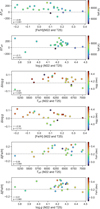 |
Fig. B.2 Residuals between our this work and literature values from Magrini et al. (2022) and Tsantaki et al. (2025) as a function of the literature values. Points are colour-coded by our derived value of the parameter shown on the y-axis. Pearson correlation coefficients (r) and p-values are annotated in each subplot. |
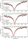 |
Fig. B.3 Simultaneous continuum and Teff Balmer line fits for KELT-21. The continuum is modelled as a second-degree polynomial. From top to bottom, the panels show Hδ, Hγ and Hβ. |
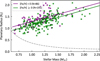 |
Fig. B.4 Planetary radius as a function of stellar mass for giant planets (Mp > 0.2 MJ and Rp > 0.6 RJ), split by stellar metallicity. Purple and green points show planets orbiting metal-poor ([Fe/H]< 0) and metal-rich ([Fe/H]≥ 0) stars, respectively; solid lines indicate the corresponding linear fits. The grey dashed curve illustrates the qualitative scaling of a fixed transit depth with stellar mass (assuming R* ∞ MJ). This curve is intended to show the decreasing detectability of small planets around more massive stars and does not represent a strict survey detection limit. |
 |
Fig. B.5 Planet density as a function of intercepted stellar power. Filled circles mark low-mass planets (not included in the fit), while outlined symbols indicate the high-mass planet subset (0.2 < Mp < 13 MJup) used for the power-law regressions. Points are colour-coded by host-star metallicity. Blue and red lines represent the best-fit relations for high-mass planets orbiting metal-poor ([Fe/H] < 0) and metal-rich ([Fe/H] ≥ 0) hosts, respectively. Right: Normalised kernel-density distributions of the giant-planet densities for the two metallicity bins. |
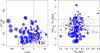 |
Fig. B.6 Left: Toomre diagram with dashed and solid lines indicating |Vtot| = 50 and 70 km s−1, respectively, used to separate thin disc, thick disc, and intermediate populations. Right: Orbital parameter space showing the difference between mean and current Galactocentric radius (Rmean – RGC) as a function of RGC. The hot star sample is shown in red and the T25 comparison sample in blue; the symbol size scales with orbital eccentricity. |
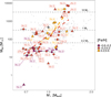 |
Fig. B.7 Total planetary mass available in each planetary system (circle), as a function of the stellar mass, colour-coded by the stellar [Fe/H]. Triangles represents those systems for which we could only determine a lower limit of the total mass. Gray dots represents the mass of planets in single planet systems. Dashed lines are plotted to provide a visual range of masses in term of MJ. The black cross identifies the Solar System and stellar mass errors are reported for each system. |
All Tables
All Figures
|
Fig. 1 Kiel diagram of analysed stars. Stars analysed in this work are shown as blue dots, those from M22 as orange stars, and those from T25 as green symbols. The two grids correspond to PARSEC isochrones with ages from 0.1 to 14 Ga, in steps of 0.05 Ga, at solar metallicity (Z = 0.013, in purple) and at super-solar metallicity (Z = 0.06, in pink). The cross in the lower left corner indicates representative 1σ uncertainties for this work (ΔTeff = 110 K and Δ log g = 0.04 dex). |
| In the text | |
|
Fig. 2 Schematic overview of iterative spectro-trigonometric analysis. Boxes represent individual analysis steps, with updated parameters listed below the horizontal line. Arrows indicate the workflow from top to bottom. Effective temperatures and initial surface gravities were constrained from Balmer line wings, trigonometric surface gravities were derived from stellar mass, bolometric magnitude, and temperature, and metal lines were used to refine all remaining atmospheric parameters until convergence was achieved. |
| In the text | |
|
Fig. 3 Left panels : normalised residuals defined as the difference between this work’s estimates and previous ones, divided by the propagated uncertainty of both estimates plotted against previous estimates from M22 and T25. Outliers are defined as stars with normalised residuals lying outside the 3σ region, marked by the dashed red lines. Orange points indicate the 5 stars from T25 for which Teff is above 3σ. Median and median absolute deviation (MAD) values are indicated in each panel. Right panels : distribution of normalised residuals. The red curve shows a standard normal distribution (mean zero, variance one) to ease visual assessment of consistency between works. |
| In the text | |
|
Fig. 4 Distributions of homogeneously derived stellar parameters for the Ariel mission candidate sample. The red histograms represent the stars analysed in this work, while the filled blue bins show results from our previous analysis (T25 and M22). |
| In the text | |
|
Fig. 5 Microturbulent velocity as a function of Teff. Red points are stars from this analysis and blue points are stars from M22 and T25. |
| In the text | |
|
Fig. 6 Projected rotational velocity (v sin i) as a function of stellar mass, colour-coded by effective temperature. Hot fast rotators analysed in this work are highlighted with a black circle. |
| In the text | |
|
Fig. 7 Left panels : same as in Fig. 3, but for 18 hot stars. Literature values are from Hartman et al. (2015); Zhou et al. (2019b); Jones et al. (2019); Niemczura et al. (2017); Johnson et al. (2018); Kama et al. (2023); Addison et al. (2021); Cabot et al. (2021); Hellier et al. (2019b,a); Lendl et al. (2020); Psaridi et al. (2023); Saffe et al. (2021), and Saffe et al. (2022). Right panels : distribution of normalised residuals. The red curve shows a standard normal distribution (mean zero, variance one). |
| In the text | |
|
Fig. 8 Host star metallicity distributions for Ariel target candidate sample systems with low-mass planets (Mp < 0.2 MJ; yellow) and high-mass planets (Mp ≥ 0.2MJ; green). Solid vertical lines mark the median [Fe/H] values, and the dotted lines indicate the 95% confidence intervals. |
| In the text | |
|
Fig. 9 Planet density as a function of stellar mass. The points are colour-coded by semi-major axis (AU), with a logarithmic colour scale. Solid and dashed black lines show linear fits for high- and low-metallicity hosts ([Fe/H] ≥ 0 and < 0, respectively), considering only planets more massive than 0.2 MJ. Following the compositional density divisions from Zeng et al. (2019), we indicate reference lines at ρ ~ 1, 3.3, and 8 g cm−3 corresponding respectively to a water- or ice-rich, silicate-rocky, and iron-rich bulk composition. Black circles highlight the 18 stars analysed in this work. |
| In the text | |
|
Fig. 10 Total planetary mass available in each planetary system, as a function of the stellar mass (with error bars), colour-coded by the ML metric (see main text). The grey dots represents the mass of planets in single planet systems. Dashed lines are plotted to provide a visual range of masses in terms of MJ. The black cross identifies the Solar System and stellar mass errors are reported for each system. |
| In the text | |
|
Fig. 11 Multiplicity distribution (left panel) and distribution of the eccentricity of each largest body in the system (right panel). Each distribution is colour-coded based on the total mass bins: low-mass, mid-mass, and high-mass (see text for more details). Dashed line marks the eccentricity value of e = 0.1 (see text for more details). |
| In the text | |
|
Fig. 12 Semi-major axis of the largest body in the system, as a function of the host stellar mass, and colour-coded by the total mass in each system. The dashed regression lines are plotted for trend identification purposes. Labels indicate the multiplicity, N, and the eccentricity for each planet. Stellar mass and semi-major axis errors are reported for each system. |
| In the text | |
|
Fig. A.1 Examples of log g f corrections calibrated using the Sun, Procyon, and 21 Peg. The black line shows the observed spectrum, the red line the synthetic spectrum computed with the original VALD3 log gf values, and the blue line the final corrected model. Only lines for which log gf values were adjusted are labelled, while small ticks mark the positions of unmodified lines. |
| In the text | |
|
Fig. B.1 Observed, synthetic, and difference spectra (black, red, blue lines) for stars in the sample, sorted by ν sin i from left bottom to top right. |
| In the text | |
|
Fig. B.2 Residuals between our this work and literature values from Magrini et al. (2022) and Tsantaki et al. (2025) as a function of the literature values. Points are colour-coded by our derived value of the parameter shown on the y-axis. Pearson correlation coefficients (r) and p-values are annotated in each subplot. |
| In the text | |
|
Fig. B.3 Simultaneous continuum and Teff Balmer line fits for KELT-21. The continuum is modelled as a second-degree polynomial. From top to bottom, the panels show Hδ, Hγ and Hβ. |
| In the text | |
|
Fig. B.4 Planetary radius as a function of stellar mass for giant planets (Mp > 0.2 MJ and Rp > 0.6 RJ), split by stellar metallicity. Purple and green points show planets orbiting metal-poor ([Fe/H]< 0) and metal-rich ([Fe/H]≥ 0) stars, respectively; solid lines indicate the corresponding linear fits. The grey dashed curve illustrates the qualitative scaling of a fixed transit depth with stellar mass (assuming R* ∞ MJ). This curve is intended to show the decreasing detectability of small planets around more massive stars and does not represent a strict survey detection limit. |
| In the text | |
|
Fig. B.5 Planet density as a function of intercepted stellar power. Filled circles mark low-mass planets (not included in the fit), while outlined symbols indicate the high-mass planet subset (0.2 < Mp < 13 MJup) used for the power-law regressions. Points are colour-coded by host-star metallicity. Blue and red lines represent the best-fit relations for high-mass planets orbiting metal-poor ([Fe/H] < 0) and metal-rich ([Fe/H] ≥ 0) hosts, respectively. Right: Normalised kernel-density distributions of the giant-planet densities for the two metallicity bins. |
| In the text | |
|
Fig. B.6 Left: Toomre diagram with dashed and solid lines indicating |Vtot| = 50 and 70 km s−1, respectively, used to separate thin disc, thick disc, and intermediate populations. Right: Orbital parameter space showing the difference between mean and current Galactocentric radius (Rmean – RGC) as a function of RGC. The hot star sample is shown in red and the T25 comparison sample in blue; the symbol size scales with orbital eccentricity. |
| In the text | |
|
Fig. B.7 Total planetary mass available in each planetary system (circle), as a function of the stellar mass, colour-coded by the stellar [Fe/H]. Triangles represents those systems for which we could only determine a lower limit of the total mass. Gray dots represents the mass of planets in single planet systems. Dashed lines are plotted to provide a visual range of masses in term of MJ. The black cross identifies the Solar System and stellar mass errors are reported for each system. |
| In the text | |
Current usage metrics show cumulative count of Article Views (full-text article views including HTML views, PDF and ePub downloads, according to the available data) and Abstracts Views on Vision4Press platform.
Data correspond to usage on the plateform after 2015. The current usage metrics is available 48-96 hours after online publication and is updated daily on week days.
Initial download of the metrics may take a while.