| Issue |
A&A
Volume 709, May 2026
|
|
|---|---|---|
| Article Number | L1 | |
| Number of page(s) | 6 | |
| Section | Letters to the Editor | |
| DOI | https://doi.org/10.1051/0004-6361/202660003 | |
| Published online | 30 April 2026 | |
Letter to the Editor
The spectrum of the persistent radio source associated with FRB 20190417A
1
Istituto Nazionale di Astrofisica – Istituto di Radioastronomia, Via Gobetti 101, 40129 Bologna, Italy
2
South African Radio Astronomy Observatory, Cape Town, 7700, South Africa
3
Centre for Radio Astronomy Techniques and Technologies (RATT), Department of Physics and Electronics, Rhodes University, Makhanda 6140, South Africa
4
Istituto Nazionale di Astrofisica – Osservatorio Astronomico di Cagliari, Via della Scienza 5, I-09047 Selargius (CA), Italy
5
Dipartimento di Fisica e Astronomia – Università di Bologna, Via Gobetti 93/2, 40129 Bologna, Italy
6
Scuola Universitaria Superiore IUSS Pavia, Palazzo del Broletto, piazza della Vittoria 15, I-27100 Pavia, Italy
★ Corresponding author: This email address is being protected from spambots. You need JavaScript enabled to view it.
Received:
23
March
2026
Accepted:
13
April
2026
Abstract
Context. Persistent radio sources (PRSs) are (sub-)parsec-scale compact non-thermal continuum sources associated with some repeating fast radio bursts (FRBs). Their nature is debated, but their properties provide insights into the FRB environment and progenitors.
Aims. We measure the spectrum of the recently confirmed PRS associated with FRB 20190417A. Spectral features such as the self-absorption and cooling break can be used to constrain the age and size of PRSs and test theoretical models.
Methods. We present observations made at 1.26 GHz with the upgraded Giant Metrewave Radio Telescope (uGMRT) and observations at 6 GHz made with the Karl Jansky Very Large Array (VLA). With complementary archival data and the LOw Frequency ARray Two Meter Sky Survey (LoTSS), we characterise the spectrum of the PRS between 144 MHz and 6 GHz.
Results. The spectrum follows a power-law behaviour at gigahertz frequencies. The source is not detected at 144 MHz down to a 2σ = 170 μJy sensitivity. We modelled the spectrum with a broken power law, obtaining a spectral index α = 0.20 ± 0.05 between 1–6 GHz. We placed a lower limit on the turn-over frequency of > 370 MHz (95% confidence).
Conclusions. The flat spectrum and low-frequency turn-over of the target are consistent with the spectral properties predicted for magneto-ionic nebulae, inflated behind the supernova ejecta by a flaring young magnetar. Considering the multi-zone magnetar wind nebula scenario, we estimate an age of t < 250 yr and a radius of R < 0.4 pc for the target, which would thus be slightly older than the PRSs associated with FRB 20121102A and FRB 20190520B.
Key words: radiation mechanisms: non-thermal / radio continuum: general
© The Authors 2026
 Open Access article, published by EDP Sciences, under the terms of the Creative Commons Attribution License (https://creativecommons.org/licenses/by/4.0), which permits unrestricted use, distribution, and reproduction in any medium, provided the original work is properly cited.
This article is published in open access under the Subscribe to Open model. This email address is being protected from spambots. You need JavaScript enabled to view it. to support open access publication.
1. Introduction
Fast radio bursts (FRBs; Lorimer et al. 2007) are bright (Jansky-level) flashes with a short duration (∼1 ms) mostly originating at extragalactic distances, whose nature is still debated (e.g. Cordes & Chatterjee 2019; Petroff et al. 2019; Bailes 2022; Zhang 2023, for reviews). Thousands of FRBs are known today, with a small fraction (∼2%) of them showing repeating activity (Chime/FRB Collaboration 2019, 2026). It is unclear whether the dichotomy between repeating and non-repeating FRBs is genuine or is the result of observational limits, implying that all FRBs can repeat on sufficiently long timescales (e.g. Chime/FRB Collaboration 2023; Kirsten et al. 2024).
A handful of repeating FRBs (FRB 20121102A, FRB 20190520B, FRB 20240114A, and FRB 20190417A) is spatially coincident with persistent radio sources (PRSs), which are compact objects on (sub-)parsec scales emitting continuum non-thermal radiation (Chatterjee et al. 2017; Marcote et al. 2017; Niu et al. 2022; Bhandari et al. 2023; Ibik et al. 2024; Bhusare et al. 2025; Bruni et al. 2025; Moroianu et al. 2026). A candidate PRS is also associated with FRB 20201124A (Bruni et al. 2024), but its size is poorly constrained (< 700 pc).
The engine powering PRSs and the mechanisms triggering FRBs are still unclear. A linear correlation was observed between the rotation measure (RM) of the FRB and the spectral luminosity (Lν) of the associated PRS (Yang et al. 2020b; Bruni et al. 2024), which suggests that relativistic electrons powering synchrotron emission and thermal electrons causing Faraday rotation coexist within a strongly magnetised environment. In this framework, magnetar wind nebulae (MWNe; Margalit & Metzger 2018) and nebulae arising from hyper-accreting X-ray binaries (Sridhar & Metzger 2022) have been proposed as promising PRS engines. Alternatively, PRSs might be associated with core-dominated active galactic nuclei (AGN) from accreting intermediate-mass (M ∼ 102 − 105 M⊙) black holes (IMBHs; e.g. Anna-Thomas et al. 2023; Dong et al. 2024).
The spectral properties (spectral index, turn-over, and break frequency) can be used to constrain the origin of PRSs (e.g. Vohl et al. 2023; Balasubramanian et al. 2025; Bhattacharya et al. 2025; Rahaman et al. 2025). In this Letter, we report on spectral measurements of the PRS associated with FRB 20190417A (Ibik et al. 2024; Moroianu et al. 2026) by employing upgraded Giant Metrewave Radio Telescope (uGMRT) and Karl Jansky Very Large Array (VLA) data covering a frequency range of 1–8 GHz, and LOw Frequency ARray (LOFAR) data at 144 MHz.
Throughout this paper, we adopt a standard ΛCDM cosmology with H0 = 70 km s−1 Mpc−1, ΩM = 0.3, and ΩΛ = 0.7. We adopt the convention on the spectral index α as defined from the flux density as Sν ∝ ν−α. The paper is organised as follows. In Sect. 2 we summarise the literature on the target. In Sect. 3 we present the analysed radio data. In Sect. 4 we derive the spectral properties of the PRS. In Sect. 5 we discuss our results.
2. The PRS associated with FRB 20190417A
The source FRB 20190417A (RA = 19h 39m 05.89s, Dec = 59° 19′ 36.83″) is a repeating FRB with high dispersion measure DM = 1378 pc cm−3 (Fonseca et al. 2020; Michilli et al. 2023), whose position is known at milliarcsec precision (Moroianu et al. 2026). The source shows a high rotation measure RM ∼ 4500 rad m−2 (Mckinven et al. 2023) with ∼20% variations on timescales of a few months (Moroianu et al. 2026). The FRB is associated with a dwarf (M ∼ 7.6 × 10⁷ M⊙) low-metallicity (Z ∼ 0.2 Z⊙) star-forming galaxy (SFR ∼ 0.2 M⊙ yr−1) at redshift z = 0.12817 (Ibik et al. 2024; Moroianu et al. 2026).
A candidate PRS with a flux density of S1.52 = 173 ± 9 μJy and compact down to a resolution of 1.3″ × 1.1″ was reported by Ibik et al. (2024) at 1.52 GHz. Moroianu et al. (2026) confirmed the association with the FRB and the compactness down to a resolution of 0.033″ × 0.031″ (implying a size < 23 pc), measuring S1.4 = 190 ± 40 μJy.
The field of FRB 20190417A is included in a sample of 24 FRBs observed in the continuum with uGMRT in band 5 (1060–1460 MHz) to search for possible PRSs (Pelliciari et al., in prep.). The associated PRS was also followed up with the VLA in C band (4–8 GHz) in B configuration.
3. Observations and data processing
In this section, we present new observations of the PRS associated with FRB 20190417A taken with the uGMRT at 1.26 GHz and with the VLA at 6 GHz. We also reprocessed one of the six VLA observations at L band (1–2 GHz) presented by Ibik et al. (2024). The details of the observations are listed in Table 1.
Details of the radio data.
We carried out a standard data reduction with the Common Astronomy Software Applications (CASA; McMullin et al. 2007) v. 6.7 for all observations. After flagging data corrupted by RFI, we obtained delay, bandpass, and amplitude solutions from the primary calibrator and complex gain solutions from the secondary calibrator (Table 1). The flux density scale was set accordingly with Perley & Butler (2017), with uncertainties < 5%. We additionally performed a round of phase self-calibration for the uGMRT data to improve the image quality. Imaging was performed with WSClean (Offringa et al. 2014; Offringa & Smirnov 2017) v. 3.6 with a multi-frequency synthesis algorithm.
In addition, we retrieved three observations from the VLA Sky Survey (VLASS; Lacy et al. 2020) at S band (2 − 4 GHz) in B configuration, with a resolution of θ ∼ 2.5″. Each epoch has a σ = 120 μJy beam−1 rms noise. After convolving these images with a θ = 3″ × 3″ beam, we averaged them and reached σ = 75 μJy beam−1 in the stacked image.
Finally, the field of FRB 20190417A was covered by the Third Data Release of the LoFAR Two Meter Sky Survey (LoTSS-DR3; Shimwell et al. 2026) at 120–168 MHz. The 144 MHz image at θ = 6″ has a noise of σ = 85 μJy beam−1.
4. Results
We show the uGMRT and VLA images in Fig. 1 and summarise their properties in Table 2. The PRS is detected in all these images with a high signal-to-noise ratio (S/N ∼ 8 − 18). A low-significance (2σ) peak is also detected in the VLASS image, but is not detected in the LoTSS image (Fig. A.1).
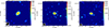 |
Fig. 1. Images of the PRS. From left to right: uGMRT at 1.26 GHz, VLA at 1.52 GHz, and VLA at 6 GHz. The resolution and noise are reported at the top of each panel. The contour levels are [ ± 3, 6, 12]×σ. |
4.1. Flux density measurements
We performed a Gaussian fit to the surface brightness of the PRS to obtain flux density measurements. The fitted peak values are reported in Table 2 (with uncertainties ΔS = σ).
Our 1.52 GHz VLA flux density is higher by a factor of 1.3 than the 1.4 GHz value reported by Moroianu et al. (2026) and derived from European Very Long Baseline Interferometry Network (EVN) observations. Although the two measurements are consistent within the uncertainties, this difference may reflect a contribution from extended emission, which remains unresolved in our arcsecond-resolution images, while it is not recovered by EVN due to its lower sensitivity at short spacings. On the other hand, we note that our S1.52 measurement is inconsistent (95% confidence) with Ibik et al. (2024). The target is located ∼10′ away from the pointing centre, where the primary beam attenuation is ∼65% (Perley 2016). When this correction is not accounted for, the two flux density measurements agree well, which might suggest that Ibik et al. (2024) did not properly account for it. As a further check, we measured S1.52 for ten compact sources in the field and compared it with S1.4 from the National Radio Astronomy Observatory VLA Sky Survey (NVSS; Condon et al. 1998). The agreement was good, with a mean S1.4 to S1.52 ratio of 1.0 (and a standard deviation of 0.3), which rules out any impacting flux scale offset in our image. In the following, we exclude S1.52 by Ibik et al. (2024) from our analysis.
4.2. Radio spectrum and spectral luminosity
The PRS flux densities (Table 2 and S1.4 by Moroianu et al. 2026) and the 2σ upper limit provided by LoTSS (S144 < 170 μJy) are shown in Fig. 2. A single power law fits observations in the 1–6 GHz range well, but the extrapolation of the spectrum at 144 MHz exceeds the upper limit by a factor of ∼2. This suggests a turn-over (νto) at low frequency.
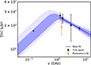 |
Fig. 2. Radio spectrum of the PRS. The flux densities (dots) and upper limit (triangle) were fitted with a broken power law (Eq. (1)) through the MCMC method. The shaded regions indicate the 68% (dark) and 95% (light) confidence levels. The posterior probability distributions of the fitted parameters (νto, S3, α) are shown in Fig. B.1. |
To model the observed spectrum, we considered a broken power law describing two optically thin regimes dominated by low-energy (S ∝ ν1/3) and high-energy (S ∝ ν−α) relativistic electrons (see Appendix B for details), in the form
![Mathematical equation: $$ \begin{aligned} S(\nu ) = {\left\{ \begin{array}{ll} S_3 \left(\dfrac{\nu }{\nu _{\rm to}}\right)^{1/3} \left(\dfrac{\nu _{\rm to}}{3\,\mathrm{GHz} }\right)^{-\alpha },&\nu < \nu _{\rm to} \\ [1.2em] S_3 \left(\dfrac{\nu }{3\,\mathrm{GHz} }\right)^{-\alpha },&\nu \ge \nu _{\rm to}, \end{array}\right.} \end{aligned} $$](/articles/aa/full_html/2026/05/aa60003-26/aa60003-26-eq1.gif) (1)
(1)
where the normalisation was set at 3 GHz as the (approximate) average frequency between 1.2 and 6 GHz. Following a Markov chain Monte Carlo (MCMC) approach, we fitted the spectrum in Eq. (1), leaving S3, νto, and α free to vary within uniform prior ranges (Appendix B).
The spectral index at gigahertz frequencies is well constrained, with a best-fit value of α = 0.20 ± 0.05. While this result differs from the steep spectrum (α ∼ 1.2) reported by Ibik et al. (2024), their measurement was derived within a narrower frequency range (1–2 GHz). We found a best-fit flux density S3 = 211 ± 8 μJy at 3 GHz, whereas we set a lower limit νto ≥ 370 MHz (95% confidence level) to the turn-over frequency. We stress that the high-frequency spectral index is robust against the choice of the upper-limit significance, while νto is more sensitive to this assumption. Specifically, a more conservative 3σ upper limit at 144 MHz would result in slightly lower turn-over frequency values (νto ≥ 300 MHz), but this difference relative to the 2σ case remains marginal.
By assuming the best-fit spectral index, we derived the k-corrected spectral luminosity as  , where DL = 601 Mpc is the luminosity distance. This yields a 1.5 GHz spectral luminosity of L1.5 = (9.5 ± 0.8)×1028 erg s−1 Hz−1.
5. Discussion and conclusions
We presented the spectrum of the PRS associated with FRB 20190417A. At 1.26–6 GHz, the spectrum follows a power law with a flat spectral index α = 0.20 ± 0.05. The PRS is not detected at 144 MHz (S144 < 170 μJy), showing a turn-over at low frequencies. We estimated the turn-over frequency to be in the range of 0.37–1.26 GHz. The source spectral luminosity at 1.5 GHz is L1.5 = (9.5 ± 0.8)×1028 erg s−1 Hz−1.
The PRSs associated with FRB 20121102A (PRS1), FRB 20190520B (PRS2), FRB 20240114A (PRS3), and FRB 20190417A (PRS4) reside in dwarf star-forming galaxies with low metallicity (Bassa et al. 2017; Niu et al. 2022; Bruni et al. 2025; Moroianu et al. 2026). These tend to exhibit flat spectra (α ∼ 0.1 − 0.4) at gigahertz frequencies and luminosities in the range Lν ∼ 1028 − 1029 erg s−1 Hz−1. Notably, PRS2 shows a turn-over below ∼1 GHz (Balasubramanian et al. 2025), similarly to PRS4. A turn-over might also exist for PRS3, but the prominent flux density variability on short timescales (Zhang et al. 2025) prevents a firm conclusion. The spectrum of PRS1 steepens at ∼10 − 20 GHz (α ∼ 1), whereas current low-frequency data down to 400 MHz do not provide solid evidence for a turn-over (Resmi et al. 2021; Bhardwaj et al. 2025).
A low-frequency turn-over, caused by synchrotron self-absorption, is predicted by the MWN model (Margalit & Metzger 2018). The MWN multi-zone model described in Rahaman et al. (2025) assumes an expanding magnetised nebula surrounded by a supernova remnant and embedding a young (∼102 yr) magnetar with a long period (∼10 ms). This model predicts a self-absorption frequency at ∼200 − 500 MHz for PRS1 and PRS2. The flat spectrum of PRS4, similar to that of pulsar wind nebulae (e.g. Gaensler & Slane 2006; Kothes 2017), and its low-frequency turn-over are consistent with the MWN model.
In conclusion, a MWN scenario is viable for PRS4. We used scaling relations from Rahaman et al. 2025 (see Appendix B) to provide limits on the radius and age of PRS4, finding R < 0.4 pc (consistent with the current limit from Moroianu et al. 2026) and t < 250 yr. In this scenario, PRS4 would thus be slightly older and more extended than PRS1 and PRS2. We note that Moroianu et al. (2026) argued that the hosts of known PRSs are thought to favour the formation of short-period (∼3 ms) magnetars, thus challenging the assumption of long-period magnetars in the model proposed by Rahaman et al. (2025). This might either indicate limitations of the multi-zone MWN model by Rahaman et al. (2025) or the need of considering alternative scenarios, such as a hyper-accreting X-ray binary system (Sridhar & Metzger 2022) or low-power and core-dominated AGN from IMBHs (Eftekhari et al. 2020; Anna-Thomas et al. 2023; Dong et al. 2024; Bhardwaj et al. 2025).
Acknowledgments
The authors thank the referee for their comments and suggestions. LB thanks A. Ibik for kindly sharing her images. The research activities described in this paper were carried out with contribution of the NextGenerationEU funds within the National Recovery and Resilience Plan (PNRR), Mission 4 – Education and Research, Component 2 – From Research to Business (M4C2), Investment Line 3.1 – Strengthening and creation of Research Infrastructures, Project IR0000026 – Next Generation Croce del Nord. The National Radio Astronomy Observatory and Green Bank Observatory are facilities of the U.S. National Science Foundation operated under cooperative agreement by Associated Universities, Inc. We thank the staff of the GMRT that made these observations possible. GMRT is run by the National Centre for Radio Astrophysics of the Tata Institute of Fundamental Research. LOFAR (van Haarlem et al. 2013) is the Low Frequency Array designed and constructed by ASTRON. It has observing, data processing, and data storage facilities in several countries, which are owned by various parties (each with their own funding sources), and that are collectively operated by the ILT foundation under a joint scientific policy. The ILT resources have benefited from the following recent major funding sources: CNRS-INSU, Observatoire de Paris and Université d’Orléans, France; BMBF, MIWF- NRW, MPG, Germany; Science Foundation Ireland (SFI), Department of Business, Enterprise and Innovation (DBEI), Ireland; NWO, The Netherlands; The Science and Technology Facilities Council, UK; Ministry of Science and Higher Education, Poland; The Istituto Nazionale di Astrofisica (INAF), Italy. This research made use of the Dutch national e-infrastructure with support of the SURF Cooperative (e-infra 180169) and the LOFAR e-infra group. The Jülich LOFAR Long Term Archive and the German LOFAR network are both coordinated and operated by the Jülich Supercomputing Centre (JSC), and computing resources on the supercomputer JUWELS at JSC were provided by the Gauss Centre for Supercomputing e.V. (grant CHTB00) through the John von Neumann Institute for Computing (NIC). This research made use of the University of Hertfordshire high-performance computing facility and the LOFAR-UK computing facility located at the University of Hertfordshire and supported by STFC [ST/P000096/1], and of the Italian LOFAR-IT computing infrastructure supported and operated by INAF, including the resources within the PLEIADI special ‘LOFAR’ project by USC-C of INAF, and by the Physics Department of Turin University (under the agreement with Consorzio Interuniversitario per la Fisica Spaziale) at the C3S Supercomputing Centre, Italy. This research made use of SAOImageDS9, developed by Smithsonian Astrophysical Observatory (Joye & Mandel 2003), APLpy, an open-source plotting package for Python (Robitaille & Bressert 2012), Astropy, a community-developed core Python package for Astronomy (Astropy Collaboration 2013, 2018), Matplotlib (Hunter 2007), Numpy (Harris et al. 2020), SciPy (Virtanen et al. 2020).
References
- Anna-Thomas, R., Connor, L., Dai, S., et al. 2023, Science, 380, 599 [NASA ADS] [CrossRef] [Google Scholar]
- Astropy Collaboration (Robitaille, T. P., et al.) 2013, A&A, 558, A33 [NASA ADS] [CrossRef] [EDP Sciences] [Google Scholar]
- Astropy Collaboration (Price-Whelan, A. M., et al.) 2018, AJ, 156, 123 [Google Scholar]
- Bailes, M. 2022, Science, 378, abj3043 [NASA ADS] [CrossRef] [Google Scholar]
- Balasubramanian, A., Bhardwaj, M., & Tendulkar, S. P. 2025, ApJ, 995, 51 [Google Scholar]
- Bassa, C. G., Tendulkar, S. P., Adams, E. A. K., et al. 2017, ApJ, 843, L8 [NASA ADS] [CrossRef] [Google Scholar]
- Bhandari, S., Marcote, B., Sridhar, N., et al. 2023, ApJ, 958, L19 [CrossRef] [Google Scholar]
- Bhardwaj, M., Balasubramanian, A., Kaushal, Y., & Tendulkar, S. P. 2025, PASP, 137, 084202 [Google Scholar]
- Bhattacharya, M., Murase, K., & Kashiyama, K. 2025, MNRAS, staf2175 [Google Scholar]
- Bhusare, Y., Maan, Y., & Kumar, A. 2025, ApJ, 993, 234 [Google Scholar]
- Briggs, D. S. 1995, Am. Astron. Soc. Meeting Abstr., 187, 112.02 [NASA ADS] [Google Scholar]
- Bruni, G., Piro, L., Yang, Y.-P., et al. 2024, Nature, 632, 1014 [CrossRef] [Google Scholar]
- Bruni, G., Piro, L., Yang, Y.-P., et al. 2025, A&A, 695, L12 [NASA ADS] [CrossRef] [EDP Sciences] [Google Scholar]
- Chatterjee, S., Law, C. J., Wharton, R. S., et al. 2017, Nature, 541, 58 [NASA ADS] [CrossRef] [Google Scholar]
- Chime/FRB Collaboration (Andersen, B. C., et al.) 2019, ApJ, 885, L24 [Google Scholar]
- Chime/FRB Collaboration (Andersen, B. C., et al.) 2023, ApJ, 947, 83 [NASA ADS] [CrossRef] [Google Scholar]
- Chime/FRB Collaboration (Abbott, T., et al.) 2026, ApJS, 283, 34 [Google Scholar]
- Condon, J. J., Cotton, W. D., Greisen, E. W., et al. 1998, AJ, 115, 1693 [Google Scholar]
- Cordes, J. M., & Chatterjee, S. 2019, ARA&A, 57, 417 [NASA ADS] [CrossRef] [Google Scholar]
- Dong, Y., Eftekhari, T., Fong, W., et al. 2024, ApJ, 973, 133 [Google Scholar]
- Eftekhari, T., Berger, E., Margalit, B., Metzger, B. D., & Williams, P. K. G. 2020, ApJ, 895, 98 [NASA ADS] [CrossRef] [Google Scholar]
- Fonseca, E., Andersen, B. C., Bhardwaj, M., et al. 2020, ApJ, 891, L6 [NASA ADS] [CrossRef] [Google Scholar]
- Gaensler, B. M., & Slane, P. O. 2006, ARA&A, 44, 17 [Google Scholar]
- Granot, J., & Sari, R. 2002, ApJ, 568, 820 [NASA ADS] [CrossRef] [Google Scholar]
- Harris, C. R., Millman, K. J., van der Walt, S. J., et al. 2020, Nature, 585, 357 [NASA ADS] [CrossRef] [Google Scholar]
- Hunter, J. D. 2007, Comput. Sci. Eng., 9, 90 [NASA ADS] [CrossRef] [Google Scholar]
- Ibik, A. L., Drout, M. R., Gaensler, B. M., et al. 2024, ApJ, 976, 199 [Google Scholar]
- Joye, W. A., & Mandel, E. 2003, ASP Conf. Ser., 295, 489 [Google Scholar]
- Kirsten, F., Ould-Boukattine, O. S., Herrmann, W., et al. 2024, Nat. Astron., 8, 337 [NASA ADS] [CrossRef] [Google Scholar]
- Kothes, R. 2017, Astrophys. Space Sci. Libr., 446, 1 [Google Scholar]
- Lacy, M., Baum, S. A., Chandler, C. J., et al. 2020, PASP, 132, 035001 [Google Scholar]
- Lorimer, D. R., Bailes, M., McLaughlin, M. A., Narkevic, D. J., & Crawford, F. 2007, Science, 318, 777 [Google Scholar]
- Marcote, B., Paragi, Z., Hessels, J. W. T., et al. 2017, ApJ, 834, L8 [CrossRef] [Google Scholar]
- Margalit, B., & Metzger, B. D. 2018, ApJ, 868, L4 [NASA ADS] [CrossRef] [Google Scholar]
- Mckinven, R., Gaensler, B. M., Michilli, D., et al. 2023, ApJ, 951, 82 [NASA ADS] [CrossRef] [Google Scholar]
- McMullin, J. P., Waters, B., Schiebel, D., Young, W., & Golap, K. 2007, ASP Conf. Ser., 376, 127 [Google Scholar]
- Michilli, D., Bhardwaj, M., Brar, C., et al. 2023, ApJ, 950, 134 [NASA ADS] [CrossRef] [Google Scholar]
- Moroianu, A. M., Bhandari, S., Drout, M. R., et al. 2026, ApJ, 996, L16 [Google Scholar]
- Niu, C. H., Aggarwal, K., Li, D., et al. 2022, Nature, 606, 873 [NASA ADS] [CrossRef] [Google Scholar]
- Offringa, A. R., & Smirnov, O. 2017, MNRAS, 471, 301 [Google Scholar]
- Offringa, A. R., McKinley, B., Hurley-Walker, N., et al. 2014, MNRAS, 444, 606 [Google Scholar]
- Perley, R. A. 2016, in Jansky Very Large Array Primary Beam Characteristics Tech. Rep. EVLA Memo EVLA Memo 195, NRAO [Google Scholar]
- Perley, R. A., & Butler, B. J. 2017, ApJS, 230, 7 [NASA ADS] [CrossRef] [Google Scholar]
- Petroff, E., Hessels, J. W. T., & Lorimer, D. R. 2019, A&AR, 27, 4 [NASA ADS] [CrossRef] [Google Scholar]
- Rahaman, S. M., Acharya, S. K., Beniamini, P., & Granot, J. 2025, ApJ, 988, 276 [Google Scholar]
- Resmi, L., Vink, J., & Ishwara-Chandra, C. H. 2021, A&A, 655, A102 [NASA ADS] [CrossRef] [EDP Sciences] [Google Scholar]
- Robitaille, T., & Bressert, E. 2012, Astrophysics Source Code Library [record ascl:1208.017] [Google Scholar]
- Sawicki, M. 2012, PASP, 124, 1208 [NASA ADS] [CrossRef] [Google Scholar]
- Shimwell, T. W., Hardcastle, M. J., Tasse, C., et al. 2026, A&A, 707, A198 [NASA ADS] [CrossRef] [EDP Sciences] [Google Scholar]
- Sridhar, N., & Metzger, B. D. 2022, ApJ, 937, 5 [NASA ADS] [CrossRef] [Google Scholar]
- Stathopoulos, S. I., Petropoulou, M., Vasilopoulos, G., & Mastichiadis, A. 2024, A&A, 683, A225 [NASA ADS] [CrossRef] [EDP Sciences] [Google Scholar]
- van Haarlem, M. P., Wise, M. W., Gunst, A. W., et al. 2013, A&A, 556, A2 [NASA ADS] [CrossRef] [EDP Sciences] [Google Scholar]
- Virtanen, P., Gommers, R., Oliphant, T. E., et al. 2020, Nat. Methods, 17, 261 [Google Scholar]
- Vohl, D., Vedantham, H. K., Hessels, J. W. T., et al. 2023, A&A, 680, A98 [NASA ADS] [CrossRef] [EDP Sciences] [Google Scholar]
- Yang, G., Boquien, M., Buat, V., et al. 2020a, MNRAS, 491, 740 [Google Scholar]
- Yang, Y.-P., Li, Q.-C., & Zhang, B. 2020b, ApJ, 895, 7 [NASA ADS] [CrossRef] [Google Scholar]
- Zhang, B. 2023, Rev. Mod. Phys., 95, 035005 [NASA ADS] [CrossRef] [Google Scholar]
- Zhang, X., Yu, W., Yan, Z., Xing, Y., & Zhang, B. 2025, ArXiv e-prints [arXiv:2501.14247] [Google Scholar]
Appendix A: LoTSS and VLASS images
In Fig. A.1 we show the LoTSS-DR3 and stacked VLASS images used in this work. The PRS is barely detected at 3 GHz and is undetected at 144 MHz.
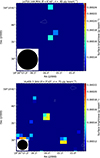 |
Fig. A.1. Images from LoTSS at 144 MHz and VLASS at 3 GHz covering the field of the PRS. The resolution and noise are reported on top of each panel. The contour levels are [ ± 2]×σ. |
Appendix B: Spectral modelling
The spectral model of the PRSs associated with FRB 20121102A and FRB 20190520B considered by Rahaman et al. (2025) to describe an expanding nebula surrounding the magnetar is based on spectrum ’1’ presented in Fig. 1 in Granot & Sari (2002). This spectrum includes four regimes determined by the self-absorption (νsa), peak (νm), and cooling break (νc) frequencies. These are i) a self-absorbed, optically thick, regime (ν < νsa) where S ∝ ν2, ii) an optically thin regime (νsa < ν < νm) dominated by low-energy relativistic electrons where  , iii) an optically thin regime (νm < ν < νc) dominated by high-energy relativistic electrons where S ∝ ν−α, and iv) a cooling-dominated regime (ν > νc) where S ∝ ν−α − 0.5. These frequencies are function of time, and they progressively shift towards lower values following the expansion of the nebula.
We aim to test the model proposed by Rahaman et al. (2025) for our target. As we have a limited number of data points, we considered a simplified model (Eq. 1) with only two regimes defined by a turn-over frequency. Although simplistic, this model is motived by available measurements, as we have no evidence of the cooling break at GHz frequencies (implying νc > 6 GHz), while at lower frequencies (< 1 GHz) we have only an upper limit. We stress that this upper limit (rather than a flux density measurement) does not allow us to distinguish between the self-absorbed and optically thin regimes, but in our model we assumed the latter because the coincidence of νsa and νm is unlikely (this condition verifies only for a short duration transition). Qualitatively, adopting a shallower slope ( ) provides a more restrictive lower limit on νto, whereas S ∝ ν2 would enable the turn-over to occur at lower frequencies.
We fitted the model in Eq. 1 to all available flux density measurements and the 144 MHz upper limit following the MCMC method through the emcee1 package. The considered likelihood function includes the contributions from both measurements and upper limits, which is
 (B.1)
(B.1)
where  are the fitting parameters and 𝒟 = (νi, Si) are the measured flux densities. We considered a standard Gaussian likelihood for detections, which is
![Mathematical equation: $$ \begin{aligned} \ln \mathcal{L} ^\mathrm{meas} = - \frac{1}{2} \sum _{i} \left[ \frac{(S_i - S_{\rm mod}(\nu _i;\boldsymbol{\vartheta }))^2}{\sigma _i^2} + \ln (2\pi \sigma _i^2) \right], \end{aligned} $$](/articles/aa/full_html/2026/05/aa60003-26/aa60003-26-eq7.gif) (B.2)
(B.2)
where Smod is the flux density predicted by the model and σi is the uncertainty on the measured flux density. The 144 MHz upper limit is taken into account through a likelihood term defined as the cumulative distribution function of a Gaussian (e.g. Sawicki 2012; Yang et al. 2020a; Stathopoulos et al. 2024), being:
![Mathematical equation: $$ \begin{aligned} \ln \mathcal{L} ^\mathrm{ul} = \ln \left\{ \frac{1}{2} \left[ 1 + \mathrm{erf} \left( \frac{S_{\rm ul} - S_{\rm mod}(\nu _{\rm ul};\boldsymbol{\vartheta })}{\sqrt{2}\,\sigma _{\rm ul}} \right) \right] \right\} \;, \end{aligned} $$](/articles/aa/full_html/2026/05/aa60003-26/aa60003-26-eq8.gif) (B.3)
(B.3)
where νul and σul are the reference frequency and rms noise of LoTSS image (Fig. A.1). We considered flat priors on ϑ, leaving the parameters free to vary in the ranges [10, 1260] MHz, [0, 1] Jy, [-2, 2] for νto, S3, and α, respectively. The resulting contour plots from the MCMC fit are shown in Fig. B.1, while the fitted spectrum is shown in Fig. 2.
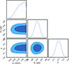 |
Fig. B.1. Posterior probability distributions of the fitted parameters (νto, S3, α) for the spectrum shown in Fig. 2. Dark and light areas refer to the 68% and 95% confidence levels, respectively. |
We used the fitted parameters to constrain the size and age of the nebula in the MWN framework, following the expressions reported in Rahaman et al. (2025). We define  ,
,  ,
,  ,
,  ,
,  , and
, and  , where ESNR is the energy of the supernova remnant (SNR) embedding the nebula and M* is the mass of the SNR progenitor. The radius and age are estimated as:
 (B.4)
(B.4)
 (B.5)
(B.5)
As fiducial assumptions, we fixed the (unknown) νc, ESNR, and M* parameters to their reference normalisation, and considered νsa = 200 MHz. By assuming values of νm = νto = 370 MHz and νc = 6 GHz (i.e. their inferred lower limits), we obtain upper limits on the radius and age of the nebula of R ≤ 0.4 pc and t ≤ 250 yr. We notice that for a lower νsa = 100 MHz, the upper limit on the age would not dramatically increase (t ≤ 400 yr). For any combination of higher values of νsa, νm, and νc, the age would be lower.
All Tables
All Figures
|
Fig. 1. Images of the PRS. From left to right: uGMRT at 1.26 GHz, VLA at 1.52 GHz, and VLA at 6 GHz. The resolution and noise are reported at the top of each panel. The contour levels are [ ± 3, 6, 12]×σ. |
| In the text | |
|
Fig. 2. Radio spectrum of the PRS. The flux densities (dots) and upper limit (triangle) were fitted with a broken power law (Eq. (1)) through the MCMC method. The shaded regions indicate the 68% (dark) and 95% (light) confidence levels. The posterior probability distributions of the fitted parameters (νto, S3, α) are shown in Fig. B.1. |
| In the text | |
|
Fig. A.1. Images from LoTSS at 144 MHz and VLASS at 3 GHz covering the field of the PRS. The resolution and noise are reported on top of each panel. The contour levels are [ ± 2]×σ. |
| In the text | |
|
Fig. B.1. Posterior probability distributions of the fitted parameters (νto, S3, α) for the spectrum shown in Fig. 2. Dark and light areas refer to the 68% and 95% confidence levels, respectively. |
| In the text | |
Current usage metrics show cumulative count of Article Views (full-text article views including HTML views, PDF and ePub downloads, according to the available data) and Abstracts Views on Vision4Press platform.
Data correspond to usage on the plateform after 2015. The current usage metrics is available 48-96 hours after online publication and is updated daily on week days.
Initial download of the metrics may take a while.