| Issue |
A&A
Volume 709, May 2026
|
|
|---|---|---|
| Article Number | A47 | |
| Number of page(s) | 15 | |
| Section | Extragalactic astronomy | |
| DOI | https://doi.org/10.1051/0004-6361/202557626 | |
| Published online | 01 May 2026 | |
A broadband study of FRB 20240114A with the Effelsberg 100-m radio telescope
1
Max-Planck-Institut für Radioastronomie, Auf dem Hügel 69, 53121 Bonn, Germany
2
Argelander Institute for Astronomy, Auf dem Hügel 71, 53121 Bonn, Germany
3
Julius-Maximilians-Universität Würzburg, Institut für Theoretische Physik und Astrophysik, Lehrstuhl für Astronomie, Emil-Fischer-Straße 31, 97074 Würzburg, Germany
4
Institute for Physics and Astronomy, University of Potsdam, 14476 Potsdam, Germany
5
Joint Institute for VLBI ERIC, Oude Hoogeveensedijk 4, 7991 PD, Dwingeloo, The Netherlands
★ Corresponding author: This email address is being protected from spambots. You need JavaScript enabled to view it.
Received:
9
October
2025
Accepted:
8
March
2026
Abstract
Context. FRB 20240114A is a hyperactive repeating fast radio burst (FRB) source discovered by the CHIME/FRB Collaboration in January 2024. The source has been followed up by numerous radio telescopes, including MeerKAT, uGMRT, and FAST, and has been localized to a dwarf star-forming galaxy at a redshift of z ∼ 0.13 with a confirmed persistent radio source.
Aims. We report observations of FRB 20240114A with the Effelsberg 100-m radio telescope using the Ultra BroadBand (UBB) receiver, covering 1.3–6.0 GHz. Over four epochs, we detected more than 700 bursts, providing an unprecedented broadband dataset for statistical analysis of this active repeater.
Methods. We performed a comprehensive study of the bursts’ morphologies, occurrence rates, spectral and temporal widths, and waiting-time distributions across six sub-bands spanning the UBB frequency range.
Results. The bursts exhibit four main spectral morphologies, including simple, complex, and frequency-drifting structures. No bursts were detected across the full 1.3–6 GHz band, confirming band-limited emission. Burst widths show modest frequency evolution, while fractional bandwidths remain roughly constant at ∼10%. Burst rates vary strongly with time and frequency, partly influenced by scintillation. The waiting-time distribution is bimodal, with largely independent bursts and short-timescale clustering on ∼10 ms, indicating a characteristic emission timescale. The source can switch emission frequencies by ≳GHz on seconds and by ∼700 MHz on millisecond timescales, implying a highly agile emission mechanism.
Conclusions. Taken together, these results indicate that FRB 20240114A is powered by a dynamic emission mechanism capable of rapid spectral modulation. The short-timescale clustering, downward frequency drifts, and lack of separation between intra- and inter-burst intervals suggest a continuous burst behaviour arising from a common physical process. This emphasizes the importance of wideband, high-time-resolution observations to constrain emission models and reveals that even among active repeaters, individual sources can exhibit unique spectral-temporal signatures.
Key words: methods: data analysis / telescopes / stars: magnetars / stars: neutron / pulsars: general
© The Authors 2026
 Open Access article, published by EDP Sciences, under the terms of the Creative Commons Attribution License (https://creativecommons.org/licenses/by/4.0), which permits unrestricted use, distribution, and reproduction in any medium, provided the original work is properly cited.
This article is published in open access under the Subscribe to Open model.
Open access funding provided by Max Planck Society.
1. Introduction
Repeating fast radio burst (FRB) sources are a subset of the FRB population that exhibit shared observed properties (Pleunis et al. 2021a). The first known repeating FRB source, FRB 20121102A, was discovered by Spitler et al. (2014) as part of the PALFA survey with the Arecibo radio telescope (Cordes et al. 2006). This source was later identified to emit repeat bursts (Spitler et al. 2016), which on further monitoring was observed to produce thousands of bursts during episodes of high activity (see Li et al. 2021; Hewitt et al. 2022; Jahns et al. 2023). An increasing number of such sources have been discovered in recent years through surveys conducted using telescopes such as CHIME, MeerKAT, the Australian Square Kilometre Array Pathfinder, and the Deep Synoptic Array (DSA-110) (CHIME/FRB Collaboration 2021; Rajwade et al. 2022; Shannon et al. 2025; Law et al. 2024). Of the ∼900 FRBs discovered to date1, repeating bursts have been observed from ∼57 sources. Expanding the known sample of repeating FRBs is therefore critical for developing a comprehensive understanding of FRB physical properties and origins.
Individual bursts from repeating FRB sources tend to exhibit narrower emission bandwidths than those from non-repeating, or ‘one-off’ FRBs (Pleunis et al. 2021a). Despite their typically narrow emission bandwidths, repeaters have been detected over a wide range of observer-frame frequencies, from as low as 110 MHz to as high as 8.0 GHz (Pleunis et al. 2021b; Gajjar et al. 2018; Bethapudi et al. 2023). Yet, even nearly two decades after the discovery of FRBs, the nature of their progenitors remains elusive. Leading models that attempt to explain repeating FRBs invoke a magnetically powered emission mechanism, often associated with highly magnetized neutron stars such as magnetars (Kumar & Lu 2017; Lu & Kumar 2018). However, it remains unclear whether the emission arises from coherent magnetospheric processes or from external shock interactions in the surrounding plasma (Metzger et al. 2019; Beloborodov 2020; Margalit et al. 2020). As upcoming surveys promise to grow the sample of known repeaters, assembling statistically significant datasets will be essential for disentangling their emission physics. In particular, broadband and sensitive observations are key to probe their spectral and temporal properties in greater detail.
Previous studies have shown that detailed investigations of burst morphologies, rates, waiting times, and energy distributions can offer valuable insights into the emission mechanisms of repeating FRBs (e.g. Jahns et al. 2023; Kirsten et al. 2024; Ould-Boukattine et al. 2025). Notably, complex frequency-time structures, such as downward-drifting bursts, appear as recurring features among multiple repeaters (Pleunis et al. 2021a). Analyses of waiting times reveal short-timescale clustering, which suggests the presence of a characteristic emission timescale (see Jahns et al. 2023; Konijn et al. 2024). At longer timescales, the behaviour is well described by an exponential distribution, consistent with a Poissonian process (Cruces et al. 2021). Some sources, such as FRB 20180916B and FRB 20121102A, have been studied at multiple radio frequencies (Bethapudi et al. 2023; Gajjar et al. 2018). These investigations are often constrained by the limited bandwidths of individual receivers and the lack of overlapping frequency coverage. In particular, Pastor-Marazuela et al. (2021) and Bethapudi et al. (2023) demonstrated that FRB 20180916B exhibits strong frequency-dependent burst activity, emphasizing the need to capture its full spectral behaviour. These limitations underscore the importance of coordinated, simultaneous multi-frequency observations of active repeaters.
To further investigate these questions, we conducted follow-up observations of the active repeating FRB 20240114A using the 100-m Effelsberg Radio Telescope. This hyperactive repeater was discovered by the CHIME/FRB Collaboration at a central frequency of 600 MHz with a reported dispersion measure (DM) of 527.7 pc cm−3 (Shin & CHIME/FRB Collaboration 2024). Following its discovery, multiple radio facilities reported detections at or below 1.4 GHz (Panda et al. 2025; Zhang et al. 2025a; Uttarkar et al. 2024), while continued monitoring revealed increased activity at frequencies above 2 GHz (Hewitt et al. 2024; Joshi et al. 2024; Limaye & Spitler 2024). The source was first localized to the host galaxy J212739.84+041945.8 by MeerKAT (Tian et al. 2024), and later refined by the European VLBI Network (EVN) PRECISE team, which pinpointed the position to RA = 21:27:39.835, Dec = +04:19:45.634 (Snelders et al. 2024), consistent with the MeerKAT co-ordinates. Optical follow-up observations confirmed the redshift of the host galaxy to be z = 0.13 (Bhardwaj et al. 2024). Subsequent observations with the Very Long Baseline Array (VLBA) established an association between the FRB and a persistent continuum radio source (PRS), making it the fourth known FRB linked to such a source (Bruni et al. 2025). Kumar et al. (2024) and Panda et al. (2025) independently report the detection of multiple repeat bursts from the source using the upgraded Giant Metrewave Radio Telescope (uGMRT). Both observing campaigns find that the burst properties vary with time. In particular, Panda et al. (2025) show that the isotropic energy distribution of the bursts follows a log-normal distribution, a behaviour often observed in pulsar single-pulse energy distributions (see Burke-Spolaor et al. 2012). Over 11 000 bursts were detected by the Five-hundred-meter Aperture Spherical radio Telescope (FAST) over the span of 214 days (Zhang et al. 2025a). A study of energetics of these bursts by Zhang et al. (2025a) using FAST observations suggest that the magnetic dipolar energy reservoirs of highly magnetized neutron stars such as ‘magnetars’ is not sufficient to explain the total released energy of the source.
The paper is structured as follows: In Section 2, we describe the observational set-up, single-pulse search strategy, calibration procedures, and data analysis methods used to extract the properties of individual bursts. In Section 3, we present the results of our study and inn Section 4, we discuss their implications. Finally, Section 5 summarizes our findings and offers interpretations based on the observational outcomes.
2. Observations and data analysis
The CHIME/FRB collaboration discovered FRB 20240114A after detecting multiple bright bursts within a few days, prompting follow-up observations with the Effelsberg radio telescope. We monitored the source for four observing epochs, with the third epoch conducted simultaneously with XMM-Newton, enabling constraints on its X-ray to radio fluence ratio (Eppel et al. 2025). Observations targeted the MeerKAT position of the source (RA = 21:27:39.83, Dec = +04:19:46.02, Tian et al. 2024).
Data were recorded using the UBB receiver, covering 1.3–6.0 GHz with a 2.6–3.0 GHz frequency gap due to instrumental limitations. The EDD backend (Barr et al. 2023) produced 8-bit full-Stokes PSRFITS search-mode files across five sub-bands within the usable range. The first two epochs used a native time resolution of 64 μs and the last two 128 μs. All data were coherently dedispersed at the MeerKAT-derived DM of 527.7 pc cm−3 (Tian et al. 2024). Further details of the observing set-up are provided in appendix Table E.1.
Flux calibration was performed using observations of the standard calibrator source 3C48 with the PSRCHIVE software suite. Calibrator observations were only conducted during one epoch (MJD 60439), but the Effelsberg system exhibits stable systematics, so the same calibration solution was applied to all epochs. The resulting system equivalent flux densities (SEFDs) are summarized in appendix Table E.1.
2.1. Single pulse search
Each EDD sub-band PSRFITS file was searched independently using the single-pulse search software TransientX (Men & Barr 2024), which is optimized for efficient processing of large datasets. A detection threshold of S/N > 7 was applied, and the resulting candidates were refined using replot_fil before final visual inspection. The full search procedure, including details of downsampling, RFI mitigation, dedispersion, and clustering strategies, is described in Appendix A.
Since each EDD sub-band was searched independently, a single burst could appear in multiple adjacent sub-bands. To identify unique events, all detections were referenced to the top of the UBB band (6.0 GHz). Assuming a temporal uncertainty of approximately 10 ms–comparable to the typical burst duration–we clustered detections across sub-bands occurring within this window. This procedure yielded a final list of unique bursts for each observing epoch, which is summarized in Table 1. We note that the burst detection statistics reported in this work differ slightly from those presented by Eppel et al. (2025), as we adopt a more conservative selection to enable a robust statistical analysis (see Section 3.2).
Effelsberg observations of FRB 20240114A with the UBB receiver.
2.2. Burst properties
We extracted burst archives using their times of arrival (TOAs) from TransientX candidates, dedispersed to a fixed DM of 527.979 pc cm−3 using DSPSR at a temporal resolution of 0.5 ms. To mitigate RFI, we applied manual masks, a zero-DM filter (up to Band 3), and CLFD (Morello et al. 2019). Flux calibration was performed using observations of the quasar 3C48, processed via PSRCHIVE.
Burst dynamic spectra and temporal profiles were reconstructed from calibrated archives (see Fig. 1). Bandwidths were visually estimated due to RFI contamination in lower bands. A multi-Gaussian fitting procedure was applied to characterize burst widths, sub-components, TOAs, and fluences. Further methodological details and a catalogue of derived properties are provided in Appendix B.
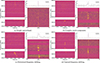 |
Fig. 1. Example dynamic spectra of selected bursts from FRB 20240114A, illustrating the distinct morphologies discussed in Section 4.1. In each subplot, the left panel shows the burst spectrum across the full UBB frequency range, where the vertical dashed lines indicate the re-binned frequency bands, while the right panel presents the dynamic spectrum (bottom) in the UBB band where the burst is detected, together with its frequency-averaged temporal profile (top). The temporal profiles are fitted with solid red curves, with dashed vertical lines marking the measured burst widths. The burst spectra were generated at a frequency resolution of 1 MHz and a time resolution of 0.5 ms. Channels affected by RFI were masked and replaced by median values for visualization. See Section 2.2 for details of the fitting methodology. |
3. Results
As is described in appendix Table E.1, the UBB sub-bands have different bandwidths. We therefore re-binned the dynamic spectra into six bands (RB1 to RB6) with approximately comparable bandwidths (see Table 2). This scheme ensured a sufficient number of bursts in each band for meaningful statistics. The SEFDs at these binned bands were computed by interpolating the SEFDs derived for the native bands from the flux calibration. The bursts were assigned to a re-binned band if their centre frequency lay within the frequency range of that band. Owing to the instrumental band gap mentioned in Section 2, bursts with centre frequencies falling within this gap were assigned to either RB2 or RB3, depending on which band was closer to the burst’s estimated centre frequency.
Frequency sub-bands and SEFD values for the UBB receiver.
3.1. Spectro-temporal properties
3.1.1. Burst morphologies
We manually classified the detected bursts into four primary morphological categories based on their frequency–time structure, as is illustrated in Fig. 1: (1) simple narrowband, (2) complex multi-component, (3) downward frequency drifting, and (4) upward frequency drifting. We did not detect any bursts emitting over the full frequency coverage of the UBB receiver. In epochs 2 and 3, we also observe a large sample of bursts above a frequency of 3 GHz, with two bursts extending up to the edge of our observing band up to a frequency of 6 GHz. This also suggests that the emission from this FRB may persist to even higher frequencies.
Quantitatively, simple narrowband bursts dominate the sample, comprising ∼73% of detections. Complex multi-component bursts account for ∼6%. Downward-drifting bursts constitute ∼20%, while upward-drifting bursts are rare (∼1.2%). Approximately 19% of bursts detected at lower frequencies (RB1–RB3) show detectable drifts, compared to only ∼6% at higher frequencies (RB4–RB6). Notably, panel (d) of Fig. 1 shows an upward-drifting burst that also includes a weak, closely spaced component just below the receiver band gap, illustrating that multiple drifting behaviours can occur on short timescales within a single event.
Figure 2 summarizes the morphological and spectral properties in the last three observing epochs; the first epoch is excluded due to the insignificant number of detected bursts. We also show the burst morphology distribution per band combined from all observing epochs in appendix Table F.1.
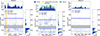 |
Fig. 2. Frequency extent of bursts from FRB 20240114A as a function of time for Epochs 2–4. Each vertical line represents an individual burst, colour-coded by morphology: simple (blue), complex multi-component (yellow), and drifting (green). The shaded regions indicate flagged frequency ranges due to RFI (light purple) and the instrumental band gap (grey). Side panels show stacked histograms of burst morphologies as a function of time (top) and frequency (right). (An artificial temporal gap is visible in Epoch 2 near 2000 s due to a technical fault during the observation.) |
The main panels of Fig. 2 show the frequency extent of each burst as a function of time, colour-coded by morphology. The instrumental band gap (shaded grey region) and persistently contaminated RFI regions (light purple) are also marked and introduce apparent cut-offs near the edges of the flagged frequencies. The side and top panels display the spectral and temporal distributions of bursts grouped by morphology. Due to the limited number of upward-drifting bursts, we combined both upward and downward drifters into a single ‘drifting’ category. We find no evidence of temporal correlations between burst morphology and frequency extent. The observed distributions are influenced by instrumental effects, such as bursts detected across the band gap and apparent cut-offs near 2.4 GHz due to RFI contamination.
3.1.2. Burst widths
We measured burst temporal widths in each resampled UBB band by fitting coherently dedispersed temporal profiles (Section 2.2). The resulting width distributions are shown as violin plots in Fig. 3, with their means and standard deviations indicated. No additional bursts were detected in the highest-time-resolution search (Appendix A), indicating that the lower tail of the width distribution is intrinsic.
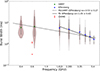 |
Fig. 3. Frequency evolution of burst widths from GMRT (green circles), Effelsberg (blue circles), and CHIME (red crosses). Distributions at each frequency are shown as violin plots in logarithmic space, with mean values and corresponding uncertainties indicated by black points with error bars. The dashed black line represents the weighted power-law fit across all frequencies (GMRT+Effelsberg), while the solid black line shows the fit using only Effelsberg data. Both fits are performed in log–log space, yielding power-law indices, α, as indicated in the legend. |
We compiled burst widths from GMRT observations reported by Panda et al. (2025), derived using the scatfit tool. Only coherently dedispersed epochs in the 300–500 MHz and 550–750 MHz bands were used. The GMRT search employed a minimum time resolution of ∼320 μs and a maximum width of 32 ms.
Two burst widths derived from CHIME baseband data (Shin et al. 2026) using fitburst are also shown. These correspond to the two brightest detected bursts and are insufficient for a statistical comparison.
A weighted power-law fit of the form W ∝ να was performed in log–log space using the GMRT and Effelsberg data, weighting each point by the standard deviation of the corresponding width distribution. The best-fit slope is α = −0.5 ± 0.3. Restricting the fit to Effelsberg data alone yields α ∼ −1.0 ± 0.6.
3.1.3. Fractional bandwidths
The burst bandwidth is defined as the visually identified frequency range of emission, and the fractional bandwidth as the ratio of this bandwidth to the burst centre frequency. Fractional bandwidth distributions are shown in Fig. 4. Across all bands, bursts from FRB 20240114A preferentially occupy fractional bandwidths of ∼10%.
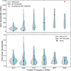 |
Fig. 4. Top: distribution of raw burst bandwidths in each frequency band shown as violin plots. Grey violins correspond to measured bursts, while blue violins show RFI-extended bursts. The red diamonds mark the scintillation bandwidth predicted by the NE2001 model. Bottom: fractional bandwidth distributions (burst bandwidth divided by centre frequency). Grey violins correspond to measured bursts, while blue violins show RFI-extended bursts. Black points with error bars indicate the mean ± standard deviation for the measured bursts. |
To account for persistently RFI-contaminated regions, we present two distributions: ‘Measured,’ derived directly from observed spectra, and ‘RFI-extended,’ where bursts truncated by RFI are assumed to extend to the edge of the affected region. In RB2, this shifts the peak fractional bandwidth from ∼20% to ∼30%. In RB4, the RFI-extended distribution is smoother than the measured one, which shows artificial truncation.
3.2. Broadband burst rate
Broadband observations with the UBB receiver enabled a spectral study of burst rates across a wide frequency range. We define the burst rate as the number of detected bursts per hour in a given frequency range, computed by normalizing the total burst count by the effective source time across all frequency sub-bands.
To assess potential underestimation of burst rates due to reduced sensitivity, particularly at lower frequencies affected by RFI, we injected synthetic FRB signals into the filterbank data using the FRB Faker tool (see Houben et al. 2026)2. The injected bursts had signal-to-noise ratios (S/Ns) of 7, 10, 30, or 100; widths of 0.1 ms, 1 ms, or 10 ms; and emission bandwidths spanning either the full sub-band or one quarter of the sub-band, centred at different frequency quartiles. After processing with TransientX, more than 80% of simulated bursts with S/N ≳ 10 were successfully recovered across all UBB bands.
To enable an unbiased comparison of burst rates across frequency, we computed fluence completeness limits in each UBB band using the radiometer equation for single pulses (Appendix C), assuming a fiducial burst width of 1 ms and a detection threshold of S/N ≳ 10. The interpolated SEFDs were used for each band. Persistent RFI was mitigated by identifying frequency channels flagged as RFI outliers for more than 70% of the data within a ∼30-minute PSRFITS file for each band and epoch. These channels were excluded to redefine the effective bandwidth. A script implementing this procedure is publicly available3.
In Table 1 and throughout this work, we consider only bursts above their respective fluence completeness thresholds, which are listed in Table 2. To compare burst rates across the entire UBB frequency range at similar energetics, we adopt the highest fluence completeness value, ∼0.1484 Jy ms (RB6), as a common reference threshold.
Figure 5 shows the fluence-complete burst rates as a function of frequency, along with the raw burst rates without completeness cuts for comparison. Error bars assume Poisson statistics. Hereafter, we interpret only the fluence-complete burst rates.
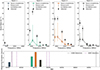 |
Fig. 5. Top panel: normalized burst count (per hour) as a function of frequency for the five UBB sub-bands over four observing epochs. For each epoch, two rate distributions are plotted: one calculated with all detected bursts and the other restricted to bursts above a common fluence threshold across all sub-bands (see Section 3.2 for details). Error bars represent uncertainties estimated from Poisson statistics, with additional error ranges overplotted to reflect expected variations due to scintillation effects (see text for details). Bottom panel: total on-source time in each observation as a function of MJD for the four UBB epochs. Vertical dashed lines indicate detection epochs reported by CHIME (black) and uGMRT (blue). |
Epoch 1 shows no detected bursts above the completeness threshold, noting that data from the four highest-frequency bands were lost and are therefore excluded. In Epoch 2, the burst rate increases significantly, particularly in RB1 and RB2, peaking near 2 GHz with a rate approximately twice that below 2 GHz. This peak is statistically inconsistent with neighboring frequency bins assuming Poisson uncertainties.
Further temporal evolution is observed in Epochs 3 and 4. Epoch 3 exhibits comparable burst rates in RB1 and RB2, with rates above 3 GHz similar to those in Epoch 2. In Epoch 4, the burst rate tentatively peaks in RB1, with substantially fewer detections at higher frequencies.
3.3. Burst waiting times
We now investigate the statistics of arrival and waiting times between consecutive bursts in our sample and their possible relation to spectral evolution. For this analysis, we focus on the first three re-binned UBB bands (RB1–RB3), in which more than 100 bursts were detected per band in total in Epochs 2 to 4, improving our statistics. We consider only the arrival times of distinct bursts when analysing wait time statistics, excluding sub-components within individual bursts. For comparison, the time separations between sub-burst components are shown using distinct histograms as depicted in Fig. 6.
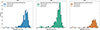 |
Fig. 6. Waiting-time distributions of bursts in the first three re-binned frequency bands (RB1–RB3, left to right). RB1 includes epochs 1–4, while RB2 and RB3 include epochs 2–4. The solid black curve shows the stacked exponential distribution using burst rates from Table H.1 for k = 1 in Equation (1). Transparent histograms indicate timescales corresponding to separations between sub-burst components of multi-component bursts. |
3.3.1. Arrival-time statistics
If the emission time of a burst is independent of any other emitted burst, the arrival times are expected to follow a Poisson distribution, while bursts whose arrival time is causally related through some process in the emission region may deviate from Poisson. We quantified the arrival-time statistics through the Weibull probability density distribution with the parametrization given in Oppermann et al. (2018):
![Mathematical equation: $$ \begin{aligned} W(\delta | k, r) = k \delta ^{-1} \left[ \delta r \Gamma (1+1/k) \right]^k e^{\left[ \delta r \Gamma (1+1/k) \right]^k }, \end{aligned} $$](/articles/aa/full_html/2026/05/aa57626-25/aa57626-25-eq1.gif) (1)
(1)
where δ are the arrival-time intervals between consecutive bursts, k is the Weibull clustering parameter, r is a constant burst rate, and Γ(x) is the gamma function. A Weibull distribution with k = 1 reduces to a Poisson distribution with a rate parameter, r. So, our primary test is whether the fitted k values are statistically consistent with k = 1. For that, we used a slightly modified version of the frb_repetition4 code from Oppermann et al. (2018).
We fitted the burst samples from individual re-binned bands and epochs separately, using only samples with > 30 bursts. Therefore, only the burst samples in RB1 and RB2 in Epochs 2, 3, and 4 and RB3 in Epochs 2 and 3 were included. (There was an observing discontinuity in Epoch 2 due to a technical glitch, and hence we excluded the bursts before this gap to avoid artificially introducing clustering). Although Cruces et al. (2021) showed that including intervals on short timescales can bias the statistics, we included all bursts in our fits. The resulting fits can be seen in Table H.1. The burst arrival times in RB1 and RB3 for all epochs considered, as well as RB2 in Epoch 3, are consistent, k = 1.0, at the 1σ level, while in RB2 for Epochs 2 and 4, the consistency is at the 2σ and 3σ levels, respectively. Therefore, in RB2 there is a greater indication of non-Poisson arrival-time statistics, but as we discuss below, this is the only band where we see short-timescale inter-burst clustering. Therefore, it is likely that these clustered bursts are pulling the fits away from the Poisson expectation.
3.3.2. Intra-band waiting-time distributions
The waiting time is defined as the time interval between two consecutive bursts within an observation, where each burst occurrence is taken to be the peak time of the highest-amplitude Gaussian component fitted to the burst profile. The waiting-time distributions for each of the three bands with all epochs combined are shown in Fig. 6 and show signs of a bi-modality particularly in RB2. The longer timescale peak (several 10s of seconds) is likely associated with bursts whose emission times are independent, and therefore are expected to follow an exponential distribution. We tested this by defining a combined exponential distribution by summing individual exponentials with rates given by the epoch-measured rate in Table 5. These estimated exponential distributions are shown by the solid black curve in Fig. 6, and it is clear that they describe the data well. To be clear, these were not fits to the histogram, but rather estimated from our rate measurements in Section 3.3.1. Therefore, we associate the longer wait time peak with independently emitted bursts.
The shorter waiting time peak, with a timescale of ≲1 s, indicates temporal clustering of bursts, distinct from the Poissonian process expected for statistically independent events as followed by the long waiting time bursts. Moreover, Fig. 6 illustrates the intervals between sub-bursts within a burst and separate bursts (inter-burst) with different transparencies. For RB1 and RB3, the only short timescale clustering are from sub-bursts, and are characterized by a timescale of a few milliseconds, i.e. similar to the characteristic duration of a single (sub-)burst. For RB2, both sub-burst and inter-burst clustering is seen on scales from a few milliseconds to of the order of 1 s, with nearly no gap between the Poisson-distributed events and the small-scale clustering. It is clear that there is a continuum of timescales between these two definitions, suggesting that the definition of burst and sub-burst is somewhat arbitrary. Therefore, the short-duration clustering timescale may be a characteristic of the emission process and similarly fundamental to the emission physics as the roughly millisecond-scale bursts.
3.3.3. Spectral-dependent waiting-time distributions
To explore whether waiting-time intervals correlate with changes in emission frequency, we define the band difference as the integer separation between re-binned frequency bands in which the centres of consecutive bursts occur. Positive (negative) values indicate upward (downward) shifts in frequency, while zero corresponds to bursts detected in the same band. Instruments with limited frequency coverage cannot detect such inter-band shifts, whereas our broadband observations capture bursts across multiple sub-bands, enabling direct study of frequency evolution with time.
Figure 7 presents a two-dimensional distribution of waiting time on the band difference. These band-resolved wait times illustrate the timescale of frequency jumps between consecutive, independent bursts. For example, a band difference of ±2 or ±5 corresponds to a frequency jump of the order of ∼ ± 1.5 GHz and ∼ ± 4 GHz, respectively. From Fig. 7 we see that frequency jumps of ±2 or ±5 bands can occur on timescales of approximately a second or tens of seconds, respectively. Therefore, the emission mechanism must be agile enough to switch frequencies separated by ≳GHz on timescales of several seconds, and a frequency of ∼700 MHz in a timescale of milliseconds.
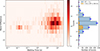 |
Fig. 7. 2D histogram (heatmap) of burst waiting times versus band differences. Waiting times are shown on a logarithmic scale, while band differences indicate jumps between observing bands. Positive values correspond to upward shifts in frequency, while negative values correspond to downward shifts. The long waiting time cluster (∼1–100 s) reflects a Poissonian process with symmetric frequency drifts, while short waiting times (≲0.1 s) show asymmetric band differences dominated by downward jumps. The vertical side panel shows time consolidated waiting-time histogram for bursts shifting towards positive (negative) frequency directions. The blue histogram corresponds to the distribution for the wait times described by a Poissonian process while the orange plot shows statistics in the short wait time cluster of bursts. The Poissonian errors on each waiting-time histogram is depicted by the scatter error bars. |
Figure 7 also shows two distinct peaks in wait time. The long waiting time cluster (∼1–100 s), which we demonstrated above to be consistent with Poisson statistics for intra-band waiting times, shows a nearly symmetric distribution of upward and downward band jumps, indicating that frequency jumps are uncorrelated on timescales ≳1 sec. This is confirmed when the 2D histogram is consolidated along the time axis (see vertical side panel in Fig. 7), which shows that the distribution of band differences for waiting times > 1 s is symmetric in positive and negative jumps.
In contrast, bursts with short waiting times (≲0.1 s) exhibit a preference for negative band differences, i.e. downward frequency drifts. Importantly, these are not merely sub-burst components but include distinct bursts detected in different frequency bands. This demonstrates that downward frequency evolution is not restricted to intra-burst structure but is also a characteristic of inter-burst clustering. This is further evidence that sub-burst and inter-burst clustering are continuum of the same emission process.
4. Discussion
4.1. Burst morphologies
Our morphological classifications are broadly consistent with those reported in CHIME/FRB Catalog 1 (Pleunis et al. 2021a) at 400–800 MHz. Although we do not observe emission across our entire frequency range corresponding to CHIME morphology type 1 (‘Simple Broadband’), this is not unexpected. Our observations are conducted at higher radio frequencies and with a larger fractional bandwidth than the CHIME/FRB survey, such that a burst appearing as broadband within the CHIME band may no longer appear as broadband when observed across a wider frequency range. Even so, we confirm that emission from repeating FRBs consistently exhibits a fractional emission bandwidth of ≲1.
Provided with the broad frequency coverage of UBB, we also studied the spectral burst properties above a frequency of 3 GHz beyond which there still is a sparse sample of FRB detections given that the current instruments perform targeted follow-up and blind searches of FRBs mostly below this frequency limit. While high-frequency emission has been reported from other repeaters–such as FRB 20121102A and FRB 20180916B in the 4–8 GHz range (Gajjar et al. 2018; Bethapudi et al. 2023)–those sources have been seen to exhibit frequency-drifting substructure extending to high frequencies. In contrast, the high-frequency bursts from FRB 20240114A presented here are relatively simple and narrowband. An inverse correlation between sub-burst drift rate and sub-component width was first identified in FRB 20121102A by Chamma et al. (2023), and subsequently validated across a broader sample of repeaters by Brown et al. (2024). This relation implies that drift rates should increase as burst durations decrease. Consistent with this trend, follow-up observations of FRB 20220912A with the Allen Telescope Array show that drift rates steepen at higher observing frequencies, while burst widths simultaneously get narrower (Sheikh et al. 2024). Under this empirical framework, the high-frequency bursts from FRB 20240114A would be expected to display large drift rates. However, as the characteristic burst widths become progressively narrow at higher frequencies, the individual sub-burst components may fall below our temporal resolution. Any intrinsic drifting behaviour may therefore be unresolved in the current data. This highlights the need for future observations with higher spectro-temporal resolution across a wide frequency range to robustly investigate the drifting behaviour of this source.
One possible interpretation of frequency drifting bursts involves evolving plasma conditions, such as decreasing particle energies or weakening magnetic fields in an expanding magnetized plasma, which can naturally produce downward drifting emission frequencies (Wang et al. 2024; Vanthieghem & Levinson 2025). Another model invokes relativistic shocks in synchrotron maser emission, where deceleration of the shock front drives a decrease in peak frequency (Metzger et al. 2019).
Alternatively, plasma lensing near the source – arising from, for example, an ionized supernova shell or the wind of a binary companion – can impose frequency-dependent magnification on the intrinsic emission. As has been shown by Main et al. (2018), such lensing can generate both upward- and downward-drifting frequency structures, depending on lens geometry and plasma density gradients. However, this scenario does not naturally explain why downward band differences dominate the clustered bursts.
Upward-drifting bursts have previously been reported in CHIME/FRB baseband data (Faber et al. 2024). Zhang et al. (2025b) analysed ∼3000 bursts from FRB 20240114A and found that the upward-drifting bursts show distinct widths, effective bandwidths, and flux densities compared to the downward-drifting ones. This suggests the possibility of different underlying emission mechanisms. Notably, the relative occurrence of upward-drifting bursts differs substantially between facilities: in the FAST sample, upward-drifting events comprise 23% of all drifting bursts, whereas in the Effelsberg sample only 6% of the drifting bursts are classified as upward-drifting. These rare upward drifts can also be likely misinterpreted as the start of one burst event at a given frequency and the end of the subsequent burst event at a higher frequency. This scenario is consistent with FAST having a higher detection rate of upward-drifting bursts, while RB2 band of Effelsberg exhibiting the most upward-drifting bursts. The example in Fig. 1 demonstrates that complex drifting behaviour can be misclassified when observed with limited bandwidth, underscoring the importance of wideband observations for accurate morphological classification.
The origin of upward-drifting bursts in the sample still remains unclear. If plasma lensing is dominant, upward and downward drifts should occur with roughly equal probability, contrary to what we observe. Presently no established model predicts upward-drifting clusters of bursts in FRBs, so we refrain from drawing strong conclusions.
4.2. Frequency-dependent burst widths
The observed inverse scaling of burst width with frequency is broadly consistent with trends reported for other repeating FRBs (Gajjar et al. 2018; Bethapudi et al. 2023). Compared to heterogeneous multi-telescope datasets, our analysis benefits from a uniform receiver system, reducing systematic uncertainties.
We note that frequency drift, which could be between sub-bursts or within a sub-burst (Jahns et al. 2023), can complicate the interpretation of a burst width if it is temporally unresolved. Unresolved drifts could broaden the frequency-averaged pulse duration, a situation that is more likely to occur at higher frequencies where the drift rates (in megahertz per millisecond) are larger (e.g. Hessels et al. 2019). This may lead to an overestimation of the burst width compared to bursts at lower frequencies, flattening the observed chromatic evolution.
Frequency-dependent evolution of burst width has been observed in other coherent emitters. The single-pulse spikes that occur within one rotational phase of the magnetar J1622−4950 show a frequency-dependent evolution in their temporal widths, modelled with a power-law index of α ∼ −0.6 ± 0.1 (Levin et al. 2012). The high-frequency interpulse (HFIP) emission of the Crab pulsar also displays notable similarities to FRBs in its spectro-temporal structure and polarization (Hessels et al. 2019). Moreover, broadband observations of the Crab pulsar by Hankins et al. (2015) show that the frequency evolution of the HFIP emission widths can be modelled with a power-law index of α ∼ −1.2 ± 0.1. This value is consistent with that derived for FRB 20240114A when considering only the Effelsberg burst sample, while the value for J1622−4950 is somewhat flatter.
The width–frequency dependence observed for FRB 20240114A may reflect intrinsic differences in emission geometry or source physics. In pulsars, radius-to-frequency mapping predicts narrower pulse profiles at higher frequencies due to emission originating closer to the neutron star surface (Cordes 1978). While Lyutikov (2017) rule out the possibility of FRBs being rotationally powered, given their very high inferred luminosities compared to the pulsar phenomena such as Crab giant pulses, similar geometric effects can still operate in magnetically powered magnetar models (Lyutikov & Rafat 2019; Lyutikov 2020).
4.3. Fractional bandwidths
The fractional bandwidths of the FRB 20240114A bursts are consistent with those observed in other repeating sources, typically spanning 10–30% of the observing frequency (Gourdji et al. 2019; Pleunis et al. 2021a; Zhang et al. 2023; Bethapudi et al. 2023). Recent theoretical work suggests that intrinsically narrowband emission may arise in magnetospheric models when the emitting region is smaller than the Doppler beaming angle, thereby suppressing geometric broadening (Kumar et al. 2024). Other models invoke quasi-periodic charge bunching or magnetospheric perturbations to produce comparably narrow spectral features (Wang et al. 2024).
In another scenario, Khangulyan et al. (2022) show that FRB emission can originate from relativistic outflows driven by energetic central engines such as magnetar flares. Building on this framework, Li et al. (2025) propose that the observed narrowband spectra of FRBs can result from synchrotron maser radiation produced in localized plasma blobs that move relativistically towards the observer within a weakly magnetized environment.
Taken together, these magnetospheric models and shock-based models both predict narrowband FRB emission. However, the relative preference for any particular mechanism remains debated. It is therefore crucial to place robust constraints on the source geometry and emission sites in order to discriminate effectively between the competing models.
4.4. Spectro-temporal burst rate evolution
A clear turnover in the burst rates was observed in Epoch 2 at a peak frequency of 2 GHz. An extensive FAST monitoring campaign at 1.1–1.5 GHz reported burst rates as high as ∼729 hr−1 above a 12σ fluence threshold of ∼0.026 Jy ms (Zhang et al. 2025a). While multiple episodes of enhanced activity were observed, no long-term rate trend was identified. During the period of heightened high-frequency activity observed in Epoch 2, contemporaneous detections above 2 GHz were also reported by the Nançay Radio Telescope and the Allen Telescope Array (Hewitt et al. 2024; Joshi et al. 2024). Below we now discuss the possible origin of these burst rate variations in the Effelsberg sample by considering effects of interstellar scintillation, intrinsic emission processes, and the complex local environment of the FRB progenitor as follows:
4.4.1. Impact of interstellar scintillation
Frequency-dependent scintillation can modulate burst fluences, boosting some bursts above the detection threshold while suppressing others. The magnification factor depends on the number of scintles (Nscint) across the emission or observing bandwidth and follows a χ2 distribution with Nd.o.f. = Nscint degrees of freedom.
The impact of scintillation is strongest when the scintillation bandwidth (Δνscint) is comparable to or larger than the emission bandwidth (Δνemit), and becomes negligible when many scintles are averaged. For FRB 20240114A, scintillation is expected to be dominated by the Milky Way foreground. Indeed, marginally resolved scintillation consistent with NE2001 predictions has been reported in the L band (Shin et al. 2026). Spectral structure consistent with scintillation is also visible in the Effelsberg bursts, though a detailed characterization is deferred to future work.
Using the NE2001 model (Cordes & Lazio 2002) and assuming a ν4 scaling, the predicted scintillation bandwidth ranges from ∼12 MHz at 1.6 GHz (RB1) to ∼1700 MHz at 6 GHz (RB6). Comparing these values with the observed emission bandwidths (Fig. 4), we find Δνemit/Δνscint ∼ 13 in RB1, ∼4 in RB2, and Δνemit ∼ Δνscint in RB3–RB6, indicating that scintillation may significantly affect observed burst rates at higher frequencies.
To estimate this effect, we combined bursts from Epochs 2–4 and recalculated rates assuming fluence thresholds of 0.04Fcomp and 2Fcomp, corresponding to the 68% confidence interval for an exponential magnification distribution (Nd.o.f. = 1). These scintillation-adjusted rates are shown in Fig. 5. While scintillation can significantly alter inferred rates, especially above 3 GHz, these estimates rely on the uncertain assumption that the completeness fluence approximates the intrinsic burst fluence and should therefore not be over-interpreted.
4.4.2. Physical origin of burst rate evolution
Assuming that the observed 2 GHz peak in Epoch 2 and the temporal evolution of burst rates reflect intrinsic source behaviour rather than propagation or instrumental effects, the time-averaged burst rate spectrum resembles gigahertz-peaked spectra (GPS) observed in some pulsars (Kijak et al. 2011) and in the magnetar XTE 1810−19 (Kijak et al. 2013; Maan et al. 2022). Such GPS-like behaviour has been attributed to chromatic variations in the source’s emission governed by complex magnetopsheric plasma processes (see Maan et al. 2022). Theoretical work suggests that variations in plasma density, magnetic field configuration, and emission altitude within a magnetar magnetosphere can produce narrowband emission whose characteristic frequency evolves with time (Kumar et al. 2024; Lyutikov 2024; Qu & Zhang 2024). In these scenarios, frequency-dependent burst rates and activity windows directly trace the underlying emission physics rather than propagation effects.
Alternatively, the GPS-like behaviour is also linked to propagation effects commonly atrributed to free–free absorption by dense ionized gas surrounding the source. Possible absorbing media include supernova remnants, pulsar wind nebulae, or H II regions, which have also been proposed as the origin of persistent radio sources (PRSs) associated with some repeating FRBs (Chatterjee et al. 2017; Niu et al. 2022). A PRS associated with FRB 20240114A has been reported by Bruni et al. (2025), showing evidence of spectral steepening between 1 and 5 GHz, while Zhang et al. (2025c) observed a continuum peak near 2 GHz. Although this continuum peak was detected roughly 2.5 months after the 2 GHz burst rate peak seen in epoch 2 of our observations, it underscores the importance of coordinated, multi-wavelength FRB observing campaigns for gaining a deeper insight into the source’s evolution.
4.5. Waiting time distribution
The results presented above reveal a complex interplay between temporal clustering and spectral evolution in the burst activity of this source. Notably, RB2 is the only band in which we detect short-timescale inter-burst clustering, a behaviour also observed in other hyperactive repeaters such as FRB 20121102A, FRB 20201124A, and FRB 20220912A (Cruces et al. 2021; Jahns et al. 2023; Zhang et al. 2022, 2023). For FRB 20240114A1, FAST observations at 1–1.5 GHz have shown a pronounced peak in short wait-time clustering at ∼34 ms (Zhang et al. 2025a), although no stable periodicity has been identified in the large sample of more than 11 000 FAST-detected bursts (Zhou et al. 2025). Interestingly, the FAST wait-time distribution exhibits a continuous bridge between the two dominant peaks, with no clear separation; this morphology is similar to what we observe in RB2, suggestive of a continuum of clustering timescales rather than distinct modes.
The lack of detectable inter-burst clustering in RB1, despite its partial overlap with the upper section of the FAST band where clustering has been observed, remains puzzling. This discrepancy may reflect intrinsic spectral variability of the source, frequency-dependent propagation effects, or sensitivity variations across our observing set-up. Additionally, uGMRT observations at 300–700 MHz show a bimodal wait-time distribution with a short-timescale peak at ∼2 ms extending out to ∼0.5 s (Panda et al. 2025). However, because those authors did not distinguish between sub-burst and inter-burst intervals, the ∼2 ms feature may be attributable to sub-burst structure rather than distinct inter-burst clustering.
Nevertheless, the coexistence of sub-burst and inter-burst clustering on a continuum of timescales in RB2 supports the interpretation that these structures likely originate from the same underlying physical mechanism, modulated by frequency-dependent emission or propagation effects. The contrasting behaviour between RB1 and RB2 underscores the importance of broadband, high-time-resolution observations to disentangle intrinsic emission physics from propagation and instrumental influences.
Wait-time statistics of Galactic magnetars provide an informative comparison. Bause et al. (2024) observed short wait-time clustering in pulses from the magnetar XTE J1810−197, including a distinct peak at the rotation period and its harmonics. Similarly, Zhu et al. (2023) conducted deep radio follow-up of SGR 1935+2154 and found that the FRB-like bursts detected from this magnetar were randomly distributed across the rotational phase rather than concentrated at a preferred longitude. They argue that such behaviour reflects temporary disturbances in the magnetosphere, which can disrupt or broaden the rotationally modulated emission window. If repeating FRBs share the same underlying mechanism, then it naturally follows that their burst activity would span a large fraction of the rotational phase, thereby suppressing or masking any detectable periodicity. This provides a plausible explanation for the persistent non-detection of rotation periods in active repeating FRBs, including FRB 20240114A.
The spectral dependence of the waiting-time behaviour shown in Figure 7 provides an additional physical insight. The symmetric pattern of frequency jumps associated with the long waiting-time bursts (≳10 s) indicates that these events are independent across the observed bands. In contrast, we identify a distinct island of clustered bursts on ∼10-ms timescales whose emission frequently shifts, with a clear preference for downward jumps. These frequency-jump intervals show no meaningful separation between intra- and inter-burst behaviour, further suggesting that a characteristic clustering timescale (∼10 ms) is fundamentally tied to the emission process. Moreover, the ability of the source to transition between frequency bands on such short timescales points to an agile and highly dynamic emission mechanism, capable of re-organising its spectral output on millisecond scales and potentially arising from distinct emitting regions within the source that dominate at different frequencies.
5. Summary and conclusions
We have presented a comprehensive wide-band study of over 700 bursts from FRB 20240114A, spanning from 1.3 to 6 GHz. The key results are summarized below:
-
Wideband data improve burst detectability and classification; narrowband observations may misclassify drifting bursts and underestimate rates.
-
No burst was detected extending across the full 1.3−6 GHz band simultaneously.
-
Two bursts were detected up to 6 GHz, the top of the receiver bandwidth.
-
Burst morphology shows significant frequency evolution, with complex, frequency-drifting structures more common at lower frequencies. No drifts are detected above 5 GHz, although narrow sub-components at these frequencies may remain unresolved given the temporal resolution of our data.
-
The fractional bandwidth remains approximately constant across observing bands, with values clustering around ∼10%. This behaviour is consistent with measurements from other repeating FRBs.
-
Burst durations were found to be narrower at higher frequencies and to have a minimal frequency dependence.
-
Burst detection rates vary strongly with both frequency and time, peaking in the 1.6–3.5 GHz range. Scintillation likely contributes to these variations, particularly above 3 GHz. A tentative spectral turnover around 2 GHz (Epoch 2) may be driven by intrinsic emission mechanism or time-variable free-free absorption caused by the complex local environment of the FRB.
-
The waiting-time distribution shows bimodality. Longer wait times are consistent with there being independent events, and also do not show any correlation with frequency. The bursts display pronounced, short-timescale frequency jumps, underscoring the remarkable agility of the emission mechanism in rapidly switching the emission over a broad range frequencies.
-
The data shows clustering over a short waiting time. These clustered bursts show a preference to jump down in frequency at these short timescales.
-
No distinction is seen in the intra- and inter-burst wait time cluster, implying that these two classes are a continuum of the same emission mechanism. The wideband wait time analysis further allows us to demonstrate this more robustly.
Compared to other known repeating FRBs, FRB 20240114A exhibits similarly complex, multi-component bursts with downward frequency drifts. With the UBB, we were able to get sensitive observations of this repeating FRB over the previously poorly sampled frequency coverage in the northern hemisphere FRB follow-up campaigns.
Overall, FRB 20240114A reinforces the diversity of repeating FRB phenomenology: while sharing many features with other active repeaters, it also exhibits source-specific spectral and temporal characteristics that provide critical constraints for emission models, in particular the rapid changes in emission frequency between independently emitted bursts. Future wideband, high-time-resolution, and polarimetric observations will be essential to further discriminate between competing physical scenarios.
Data availability
The dynamic spectra of all detected bursts, along with the burst properties listed in Table D.1 are available at the CDS via https://cdsarc.cds.unistra.fr/viz-bin/cat/J/A+A/709/A47. The flux and fluence measurements derived in this work are currently being used for a forthcoming publication but can be provided upon reasonable request to the corresponding authors.
Acknowledgments
This work is based on observations with the 100-m telescope of the MPIfR (Max-Planck Institute für Radioastronomie) at Effelsberg. The authors would like to thank Dr. Alex Kraus for scheduling observations with the new UBB receiver. The Effelsberg UBB receiver and EDD backend system are developed and maintained by the electronics division at the MPIfR. PL thanks Suryarao Bethapudi for their initial support in conducting observations and useful discussion during processing the data. LGS is a Lise Meitner Research Group Leader and acknowledges funding from the Max Planck Society. J.B. acknowledge the support by the German Science Foundation (DFG) project BE 7886/2-1. FE and MK acknowledge support from the Deutsche Forschungsgemeinschaft (DFG, grant 447572188).
References
- Barr, E. D., Bansod, A., Behrend, J., et al. 2023, 2023 XXXVth General Assembly and Scientific Symposium of the International Union of Radio Science (URSI GASS), We-J01-PM3-4 [Google Scholar]
- Bause, M. L., Herrmann, W., & Spitler, L. G. 2024, A&A, 686, A144 [NASA ADS] [CrossRef] [EDP Sciences] [Google Scholar]
- Beloborodov, A. M. 2020, ApJ, 896, 142 [NASA ADS] [CrossRef] [Google Scholar]
- Bethapudi, S., Spitler, L. G., Main, R. A., Li, D. Z., & Wharton, R. S. 2023, MNRAS, 524, 3303 [NASA ADS] [CrossRef] [Google Scholar]
- Bhardwaj, M., Kirichenko, A., & Gil de Paz, A. 2024, ATel, 16613, 1 [Google Scholar]
- Brown, K., Chamma, M. A., Rajabi, F., et al. 2024, MNRAS, 529, L152 [Google Scholar]
- Bruni, G., Piro, L., Yang, Y. P., et al. 2025, A&A, 695, L12 [NASA ADS] [CrossRef] [EDP Sciences] [Google Scholar]
- Burke-Spolaor, S., Johnston, S., Bailes, M., et al. 2012, MNRAS, 423, 1351 [Google Scholar]
- Chamma, M. A., Rajabi, F., Kumar, A., & Houde, M. 2023, MNRAS, 522, 3036 [NASA ADS] [CrossRef] [Google Scholar]
- Chatterjee, S., Law, C. J., Wharton, R. S., et al. 2017, Nature, 541, 58 [NASA ADS] [CrossRef] [Google Scholar]
- CHIME/FRB Collaboration (Amiri, M., et al.) 2021, ApJS, 257, 59 [NASA ADS] [CrossRef] [Google Scholar]
- Cordes, J. M. 1978, ApJ, 222, 1006 [NASA ADS] [CrossRef] [Google Scholar]
- Cordes, J. M., Freire, P. C. C., Lorimer, D. R., et al. 2006, ApJ, 637, 446 [NASA ADS] [CrossRef] [Google Scholar]
- Cordes, J. M., & Lazio, T. J. W. 2002, ArXiv e-prints [arXiv:astro-ph/0207156] [Google Scholar]
- Cruces, M., Spitler, L. G., Scholz, P., et al. 2021, MNRAS, 500, 448 [Google Scholar]
- Eppel, F., Krumpe, M., Limaye, P., et al. 2025, A&A, 695, L10 [NASA ADS] [CrossRef] [EDP Sciences] [Google Scholar]
- Faber, J. T., Michilli, D., Mckinven, R., et al. 2024, ApJ, 974, 274 [Google Scholar]
- Gajjar, V., Siemion, A. P. V., Price, D. C., et al. 2018, ApJ, 863, 2 [NASA ADS] [CrossRef] [Google Scholar]
- Gourdji, K., Michilli, D., Spitler, L. G., et al. 2019, ApJ, 877, L19 [NASA ADS] [CrossRef] [Google Scholar]
- Hankins, T. H., Jones, G., & Eilek, J. A. 2015, ApJ, 802, 130 [NASA ADS] [CrossRef] [Google Scholar]
- Hessels, J. W. T., Spitler, L. G., Seymour, A. D., et al. 2019, ApJ, 876, L23 [Google Scholar]
- Hewitt, D. M., Huang, J., Hessels, J. W. T., et al. 2024, ATel, 16597, 1 [Google Scholar]
- Hewitt, D. M., Snelders, M. P., Hessels, J. W. T., et al. 2022, MNRAS, 515, 3577 [NASA ADS] [CrossRef] [Google Scholar]
- Houben, L. J. M., Falcke, H., Spitler, L. G., et al. 2026, A&A, 707, A10 [NASA ADS] [CrossRef] [EDP Sciences] [Google Scholar]
- Jahns, J. N., Spitler, L. G., Nimmo, K., et al. 2023, MNRAS, 519, 666 [Google Scholar]
- Joshi, P., Medina, A., Earwicker, J. T., et al. 2024, ATel, 16599, 1 [Google Scholar]
- Khangulyan, D., Barkov, M. V., & Popov, S. B. 2022, ApJ, 927, 2 [NASA ADS] [CrossRef] [Google Scholar]
- Kijak, J., Lewandowski, W., Maron, O., Gupta, Y., & Jessner, A. 2011, A&A, 531, A16 [NASA ADS] [CrossRef] [EDP Sciences] [Google Scholar]
- Kijak, J., Tarczewski, L., Lewandowski, W., & Melikidze, G. 2013, ApJ, 772, 29 [Google Scholar]
- Kirsten, F., Ould-Boukattine, O. S., Herrmann, W., et al. 2024, Nature, 8, 337 [Google Scholar]
- Konijn, D. C., Hewitt, D. M., Hessels, J. W. T., et al. 2024, MNRAS, 534, 3331 [Google Scholar]
- Kumar, A., Maan, Y., & Bhusare, Y. 2024, ApJ, 977, 177 [Google Scholar]
- Kumar, P., & Lu, W. 2017, MNRAS, 468, 2726 [NASA ADS] [CrossRef] [Google Scholar]
- Kumar, P., Qu, Y., & Zhang, B. 2024, ApJ, 974, 160 [Google Scholar]
- Law, C. J., Sharma, K., Ravi, V., et al. 2024, ApJ, 967, 29 [NASA ADS] [CrossRef] [Google Scholar]
- Levin, L., Bailes, M., Bates, S. D., et al. 2012, MNRAS, 422, 2489 [NASA ADS] [CrossRef] [Google Scholar]
- Li, D., Wang, P., Zhu, W. W., et al. 2021, Nature, 598, 267 [CrossRef] [Google Scholar]
- Li, X., Lyu, F., Zhang, H. M., Deng, C.-M., & Liang, E.-W. 2025, A&A, 695, A100 [NASA ADS] [CrossRef] [EDP Sciences] [Google Scholar]
- Limaye, P., & Spitler, L. 2024, ATel, 16620, 1 [Google Scholar]
- Lu, W., & Kumar, P. 2018, MNRAS, 477, 2470 [Google Scholar]
- Lyutikov, M. 2017, ApJ, 838, L13 [NASA ADS] [CrossRef] [Google Scholar]
- Lyutikov, M. 2020, ApJ, 889, 135 [NASA ADS] [CrossRef] [Google Scholar]
- Lyutikov, M. 2024, MNRAS, 529, 2180 [NASA ADS] [CrossRef] [Google Scholar]
- Lyutikov, M., & Rafat, M. 2019, ArXiv e-prints [arXiv:1901.03260] [Google Scholar]
- Maan, Y., Surnis, M. P., Chandra Joshi, B., & Bagchi, M. 2022, ApJ, 931, 67 [NASA ADS] [CrossRef] [Google Scholar]
- Main, R., Yang, I. S., Chan, V., et al. 2018, Nature, 557, 522 [Google Scholar]
- Margalit, B., Beniamini, P., Sridhar, N., & Metzger, B. D. 2020, ApJ, 899, L27 [NASA ADS] [CrossRef] [Google Scholar]
- Men, Y., & Barr, E. 2024, A&A, 683, A183 [NASA ADS] [CrossRef] [EDP Sciences] [Google Scholar]
- Metzger, B. D., Margalit, B., & Sironi, L. 2019, MNRAS, 485, 4091 [NASA ADS] [CrossRef] [Google Scholar]
- Morello, V., Barr, E. D., Cooper, S., et al. 2019, MNRAS, 483, 3673 [NASA ADS] [CrossRef] [Google Scholar]
- Niu, C. H., Aggarwal, K., Li, D., et al. 2022, Nature, 606, 873 [NASA ADS] [CrossRef] [Google Scholar]
- Oppermann, N., Yu, H.-R., & Pen, U.-L. 2018, MNRAS, 475, 5109 [NASA ADS] [CrossRef] [Google Scholar]
- Ould-Boukattine, O. S., Chawla, P., Hessels, J. W. T., et al. 2025, MNRAS, 545, staf1937 [Google Scholar]
- Panda, U., Roy, J., Bhattacharyya, S., Dudeja, C., & Kudale, S. 2025, ApJ, 989, 15 [Google Scholar]
- Pastor-Marazuela, I., Connor, L., van Leeuwen, J., et al. 2021, Nature, 596, 505 [NASA ADS] [CrossRef] [Google Scholar]
- Perley, R. A., & Butler, B. J. 2017, ApJS, 230, 7 [NASA ADS] [CrossRef] [Google Scholar]
- Pleunis, Z., Good, D. C., Kaspi, V. M., et al. 2021a, ApJ, 923, 1 [NASA ADS] [CrossRef] [Google Scholar]
- Pleunis, Z., Michilli, D., Bassa, C. G., et al. 2021b, ApJ, 911, L3 [NASA ADS] [CrossRef] [Google Scholar]
- Qu, Y., & Zhang, B. 2024, ApJ, 972, 124 [Google Scholar]
- Rajwade, K. M., Bezuidenhout, M. C., Caleb, M., et al. 2022, MNRAS, 514, 1961 [Google Scholar]
- Shannon, R. M., Bannister, K. W., Bera, A., et al. 2025, PASA, 42, e036 [Google Scholar]
- Sheikh, S. Z., Farah, W., Pollak, A. W., et al. 2024, MNRAS, 527, 10425 [Google Scholar]
- Shin, K., & CHIME/FRB Collaboration 2024, ATel, 16420, 1 [Google Scholar]
- Shin, K., Curtin, A., Fine, M., et al. 2026, ApJ, 997, 334 [Google Scholar]
- Snelders, M. P., Bhandari, S., Kirsten, F., et al. 2024, ATel, 16542, 1 [Google Scholar]
- Spitler, L. G., Cordes, J. M., Hessels, J. W. T., et al. 2014, ApJ, 790, 101 [NASA ADS] [CrossRef] [Google Scholar]
- Spitler, L. G., Scholz, P., Hessels, J. W. T., et al. 2016, Nature, 531, 202 [NASA ADS] [CrossRef] [Google Scholar]
- Tian, J., Rajwade, K. M., Pastor-Marazuela, I., et al. 2024, MNRAS, 533, 3174 [NASA ADS] [CrossRef] [Google Scholar]
- Uttarkar, P. A., Kumar, P., Lower, M. E., & Shannon, R. M. 2024, ATel, 16430, 1 [Google Scholar]
- Vanthieghem, A., & Levinson, A. 2025, Phys. Rev. Lett., 134, 035201 [Google Scholar]
- Virtanen, P., Gommers, R., Oliphant, T. E., et al. 2020, Nat. Methods, 17, 261 [Google Scholar]
- Wang, W.-Y., Yang, Y.-P., Li, H.-B., Liu, J., & Xu, R. 2024, A&A, 685, A87 [NASA ADS] [CrossRef] [EDP Sciences] [Google Scholar]
- Zhang, J. S., Wang, T. C., Wang, P., et al. 2025a, ArXiv e-prints [arXiv:2507.14707] [Google Scholar]
- Zhang, L. X., Tian, S., Shen, J., et al. 2025b, ArXiv e-prints [arXiv:2507.14711] [Google Scholar]
- Zhang, X., Yu, W., Yan, Z., Xing, Y., & Zhang, B. 2025c, ArXiv e-prints [arXiv:2501.14247] [Google Scholar]
- Zhang, Y.-K., Wang, P., Feng, Y., et al. 2022, Res. Astron. Astrophys., 22, 124002 [CrossRef] [Google Scholar]
- Zhang, Y.-K., Li, D., Zhang, B., et al. 2023, ApJ, 955, 142 [NASA ADS] [CrossRef] [Google Scholar]
- Zhou, D., Wang, P., Fang, J., et al. 2025, ArXiv e-prints [arXiv:2507.14708] [Google Scholar]
- Zhu, W., Xu, H., Zhou, D., et al. 2023, Sci. Adv., 9, eadf6198 [NASA ADS] [CrossRef] [Google Scholar]
Appendix A: Single pulse search details
For the first two epochs, the data were downsampled in time by a factor of 8, and for the last two epochs by a factor of 4, for the width search from 1 ms - 40 ms in order to match the different native resolutions of the data. To mitigate narrowband RFI, the data were further downsampled in frequency by a factor of 4. We also carried out searches up to the native time resolutions to test for the presence of very narrow bursts, but no unique detections were found in this regime.
RFI mitigation in TransientX included the kadane filtering algorithm to suppress narrowband interference, complemented by manual masks to remove persistently contaminated frequency ranges. For the first three sub-bands, the zdot option was enabled to apply a zero-DM filter, removing broadband signals centred at zero DM. Additionally, zapped RFI channels were replaced with the mean of each corresponding 1 s time segment to preserve the statistical properties of the data.
Dedispersion was carried out over a DM range of 500–550 pc cm−3, with step sizes computed using DDplan.py5.
Finally, the DBSCAN clustering algorithm was used with a radius of 1 ms to merge duplicate detections across widths and adjacent trial DMs. Each resulting cluster was refined with replot_fil, which performs a high-resolution reprocessing to reduce false positives before visual inspection.
Appendix B: Methodology of burst properties extraction
The burst TOAs were extracted from TransientX candidates identified in each sub-band. To ensure consistency across frequency bands, all data were dedispersed to a fixed DM of 527.979 pc cm−3, obtained from a structure-optimized fit to a bright burst (Eppel et al. 2025). Single-pulse archives of 1-second duration were generated using DSPSR6 for all sub-bands.
RFI was mitigated using: (1) manual masks derived from folded flux calibrator archives which mask the persistently bad frequency channels, (2) a zero-DM filter for broadband RFI suppression (up to Band 3), and (3) the CLFD algorithm (Morello et al. 2019). Flux calibration used on/off scans of 3C48 with a 0.5 s diode switching period, processed using PSRCHIVE tools fluxcal and pac7 using the 3C48 calibrator model from Perley & Butler (2017).
Calibrated archives were loaded into 2D arrays via the PSRCHIVE Python Interface8. Dynamic spectra and temporal profiles were reconstructed as shown in Fig. 1. Due to significant RFI in lower-frequency bands, bandwidths were visually estimated instead of fit-based measurements.
Burst arrival times were referenced to the centre frequency of the highest band in which the burst was detected (rather than the highest channel overall, as in the initial detection). This referencing allowed us to properly handle cross-band burst detections without duplication.
Temporal structure was characterized using a multi-Gaussian fitting approach. We first smoothed the time series to identify statistically significant peaks (above a fixed S/N threshold), then fitted Gaussian components using scipy.optimize.curve_fit (Virtanen et al. 2020). Gaussian components were iteratively added until residuals converged below a reduced-χ2 threshold of 0.01.
Two components were considered sub-structures of the same burst if their FWHMs overlapped; otherwise, they were treated as distinct bursts. From the fits, we extracted FWHMs, TOAs (relative to observation start), peak flux densities (Jy), and fluences (Jy–ms). For bursts with multiple components, the effective burst widths are obtained by considering the burst envelope covered by the FWHM of the first component and the last component respectively. A catalogue of derived properties for a representative burst sample is provided in Table D.1.
Appendix C: Radiometer equation and fluence estimation
The radiometer equation for single pulses is given by
 (C.1)
(C.1)
where S is the signal’s flux density (Jy), S/N is the signal-to-noise ratio, SEFD is the system equivalent flux density (Jy), np = 2 is the number of polarizations summed, Δν is the bandwidth (Hz), and ΔW is the effective pulse width or time resolution (s).
Following this equation, the fluence ℱ (Jy ms) of a single pulse can be estimated as:
 (C.2)
(C.2)
Appendix D: Representative burst properties
Representative burst properties of FRB 20240114A.
Appendix E: Details on the receiver specifications
UBB receiver sub-band specifications from the Effelsberg EDD backend.
Appendix F: Burst morphology over the UBB frequency bands
Burst morphology counts per re-binned UBB band.
Appendix G: Burst widths across different frequencies
Mean burst widths across CHIME, GMRT, and Effelsberg frequency bands.
Appendix H: Burst rates and temporal clustering
Weibull-fitted burst rates and clustering parameters across UBB sub-bands.
All Tables
All Figures
|
Fig. 1. Example dynamic spectra of selected bursts from FRB 20240114A, illustrating the distinct morphologies discussed in Section 4.1. In each subplot, the left panel shows the burst spectrum across the full UBB frequency range, where the vertical dashed lines indicate the re-binned frequency bands, while the right panel presents the dynamic spectrum (bottom) in the UBB band where the burst is detected, together with its frequency-averaged temporal profile (top). The temporal profiles are fitted with solid red curves, with dashed vertical lines marking the measured burst widths. The burst spectra were generated at a frequency resolution of 1 MHz and a time resolution of 0.5 ms. Channels affected by RFI were masked and replaced by median values for visualization. See Section 2.2 for details of the fitting methodology. |
| In the text | |
|
Fig. 2. Frequency extent of bursts from FRB 20240114A as a function of time for Epochs 2–4. Each vertical line represents an individual burst, colour-coded by morphology: simple (blue), complex multi-component (yellow), and drifting (green). The shaded regions indicate flagged frequency ranges due to RFI (light purple) and the instrumental band gap (grey). Side panels show stacked histograms of burst morphologies as a function of time (top) and frequency (right). (An artificial temporal gap is visible in Epoch 2 near 2000 s due to a technical fault during the observation.) |
| In the text | |
|
Fig. 3. Frequency evolution of burst widths from GMRT (green circles), Effelsberg (blue circles), and CHIME (red crosses). Distributions at each frequency are shown as violin plots in logarithmic space, with mean values and corresponding uncertainties indicated by black points with error bars. The dashed black line represents the weighted power-law fit across all frequencies (GMRT+Effelsberg), while the solid black line shows the fit using only Effelsberg data. Both fits are performed in log–log space, yielding power-law indices, α, as indicated in the legend. |
| In the text | |
|
Fig. 4. Top: distribution of raw burst bandwidths in each frequency band shown as violin plots. Grey violins correspond to measured bursts, while blue violins show RFI-extended bursts. The red diamonds mark the scintillation bandwidth predicted by the NE2001 model. Bottom: fractional bandwidth distributions (burst bandwidth divided by centre frequency). Grey violins correspond to measured bursts, while blue violins show RFI-extended bursts. Black points with error bars indicate the mean ± standard deviation for the measured bursts. |
| In the text | |
|
Fig. 5. Top panel: normalized burst count (per hour) as a function of frequency for the five UBB sub-bands over four observing epochs. For each epoch, two rate distributions are plotted: one calculated with all detected bursts and the other restricted to bursts above a common fluence threshold across all sub-bands (see Section 3.2 for details). Error bars represent uncertainties estimated from Poisson statistics, with additional error ranges overplotted to reflect expected variations due to scintillation effects (see text for details). Bottom panel: total on-source time in each observation as a function of MJD for the four UBB epochs. Vertical dashed lines indicate detection epochs reported by CHIME (black) and uGMRT (blue). |
| In the text | |
|
Fig. 6. Waiting-time distributions of bursts in the first three re-binned frequency bands (RB1–RB3, left to right). RB1 includes epochs 1–4, while RB2 and RB3 include epochs 2–4. The solid black curve shows the stacked exponential distribution using burst rates from Table H.1 for k = 1 in Equation (1). Transparent histograms indicate timescales corresponding to separations between sub-burst components of multi-component bursts. |
| In the text | |
|
Fig. 7. 2D histogram (heatmap) of burst waiting times versus band differences. Waiting times are shown on a logarithmic scale, while band differences indicate jumps between observing bands. Positive values correspond to upward shifts in frequency, while negative values correspond to downward shifts. The long waiting time cluster (∼1–100 s) reflects a Poissonian process with symmetric frequency drifts, while short waiting times (≲0.1 s) show asymmetric band differences dominated by downward jumps. The vertical side panel shows time consolidated waiting-time histogram for bursts shifting towards positive (negative) frequency directions. The blue histogram corresponds to the distribution for the wait times described by a Poissonian process while the orange plot shows statistics in the short wait time cluster of bursts. The Poissonian errors on each waiting-time histogram is depicted by the scatter error bars. |
| In the text | |
Current usage metrics show cumulative count of Article Views (full-text article views including HTML views, PDF and ePub downloads, according to the available data) and Abstracts Views on Vision4Press platform.
Data correspond to usage on the plateform after 2015. The current usage metrics is available 48-96 hours after online publication and is updated daily on week days.
Initial download of the metrics may take a while.