| Issue |
A&A
Volume 709, May 2026
|
|
|---|---|---|
| Article Number | L2 | |
| Number of page(s) | 7 | |
| Section | Letters to the Editor | |
| DOI | https://doi.org/10.1051/0004-6361/202659620 | |
| Published online | 30 April 2026 | |
Letter to the Editor
Harmonic phase diagnostics of long secondary periods
Testing predictions of oscillatory convective dipole modes in the OGLE sample
1
European Southern Observatory, Alonso de Cordova 3107 Vitacura, 19001 Santiago, Chile
2
Research School of Astronomy and Astrophysics, Australian National University, Canberra 2611, Australia
3
Australian Astronomical Optics & School of Mathematical and Physical Sciences, Macquarie University, Sydney 2109, Australia
★ Corresponding author: This email address is being protected from spambots. You need JavaScript enabled to view it.
Received:
26
February
2026
Accepted:
30
March
2026
Abstract
Context. Long secondary periods (LSPs) in luminous red giants remain the only major class of long-period stellar variability without a secure physical origin. Competing hypotheses include binaries with dusty companions and oscillatory convective dipole modes.
Aims. We identified the physical and geometric conditions under which oscillatory convective dipole modes produce distinctive harmonic signatures that contrast with those expected from binary systems, and applied this diagnostic to a filtered subset of the OGLE-III LSP sample to identify examples consistent with oscillatory convective dipole modes.
Methods. We modelled the geometric flux modulation from oscillatory convective dipole modes and mapped the range of inclinations, temperature amplitudes, and observing wavelengths for which harmonic features are observable. Using OGLE-III I-band light curves, we required statistically significant power at both sequence D and its harmonic, keeping a filtered sample of 249 stars (2.1% of the ridge-selected sample). We applied iterative Lomb-Scargle and weighted Fourier decomposition to isolate the fundamental and harmonic components. The relative phase (Δϕ) between these distinguishes secondary maxima predicted by an inclined dipole from secondary minima caused by eclipsing or ellipsoidal binary systems.
Results. The majority of high amplitude stars in the filtered subset show Δϕ consistent with secondary minima produced by binary systems. However, a small but statistically non-negligible subset exhibits Δϕ consistent with secondary maxima that are difficult to reconcile by eclipsing or ellipsoidal binaries, and instead this subset matches the geometric predictions for highly inclined, non-rotating oscillatory convective dipole modes with temperature amplitudes consistent with published models.
Key words: convection / stars: AGB and post-AGB / binaries: general
© The Authors 2026
 Open Access article, published by EDP Sciences, under the terms of the Creative Commons Attribution License (https://creativecommons.org/licenses/by/4.0), which permits unrestricted use, distribution, and reproduction in any medium, provided the original work is properly cited.
This article is published in open access under the Subscribe to Open model. This email address is being protected from spambots. You need JavaScript enabled to view it. to support open access publication.
1. Introduction
Roughly one third of luminous red giants exhibit an enigmatic, long-timescale variability, commonly referred to as the long secondary period (LSP), superimposed on their primary pulsations and spanning several hundred to over one thousand days. Despite extensive study, LSPs remain the only class of large-amplitude stellar variability without a widely accepted physical explanation (Takayama & Ita 2020; Pawlak 2021; Soszyński et al. 2021). In the period–luminosity (PL) diagram of long-period variables (LPVs), LSP stars define a distinct and well-populated ridge (sequence D) (Wood et al. 1999). In contrast to other sequences, which are now understood as radial or non-radial pulsation modes (Wood et al. 2004; Trabucchi et al. 2019), Wood et al. (2004) showed that adiabatic pulsations cannot account for sequence D. Two observationally motivated hypotheses have emerged:
-
In the binary scenario the LSPs arise from a low-mass companion with dust clouds that cause periodic obscuration (e.g. Wood et al. 2004; Soszyński et al. 2021; Decin et al. 2025).
-
In the oscillatory convective mode scenario the LSPs correspond to dipole (ℓ = 1) highly non-adiabatic g-modes (e.g. Saio et al. 2015; Takayama & Ita 2020).
Recent studies have highlighted the presence of secondary minima in LSP light curves, particularly at infrared wavelengths, as compelling evidence of the binary scenario (Soszyński et al. 2021). If these systems host brown dwarf companions that have accreted from a stellar wind, there is an additional challenge in reconciling the required angular momentum with the progenitor population of giant planets (Fulton et al. 2021). Most discussions to date have focused on finding a universal mechanism, with limited attention to the possibility of multiple LSP origins coexisting across the asymptotic giant (AGB) and red giant (RGB) branch populations. In this work, we focus on a distinguishing observational feature: the presence of harmonics in sequence D stars. In binaries, these harmonics can arise from secondary eclipses, producing a phase-locked secondary minimum in the light curve as shown by Soszyński et al. (2021). However, no similar mechanism has been previously proposed to explain such harmonic structure under the oscillatory convective mode hypothesis. We show here that oscillatory dipole modes can naturally produce strong harmonics through purely geometric effects linked to viewing inclination. Crucially, these harmonics manifest not as secondary minima, but as secondary maxima in the light curve, yielding a distinctive phase offset between the fundamental and its harmonic. This provides a new diagnostic capable of separating the binary and convective-mode scenarios. We identify and analyse examples of such signatures in OGLE light curves.
2. Harmonics on sequence D
Figure 1 shows the PL diagram of LPVs in the Large Magellanic Cloud (LMC), based on the OGLE-III catalogue. The periods correspond to the dominant periodicity identified in each light curve plotted against the Wesenheit index WJK = Ks − 0.686(J − Ks). Among the known PL ridges, sequence D is populated by stars exhibiting LSPs. A secondary ridge is also visible at approximately half the period of sequence D, which we refer to here as sequence D1/2. This ridge largely overlaps with the high-amplitude regime of sequence E, commonly associated with ellipsoidal binary systems (Soszynski et al. 2004; Pawlak et al. 2014). However, detailed comparisons of photometric and radial-velocity behaviour have shown that the sequence D variability itself is not caused by ellipsoidal modulation, and that stars on sequences D and E exhibit very distinct observational properties (Nicholls et al. 2010). In the context of this work, the designation D1/2 is therefore used to emphasise the hypothesis that a subset of stars on this harmonic ridge may not be ellipsoidal or eclipsing binaries, they may instead reflect a harmonic structure arising from the same physical mechanism responsible for the sequence D signal. The joint presence of significant power on both sequence D and its harmonic is a prerequisite for applying the harmonic phase diagnostic developed below, and it does not imply that sequence D1/2 represents an independent pulsation sequence or a reinterpretation of sequence E.
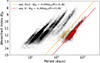 |
Fig. 1. Sequence D (red) in the PL diagram along with a sub-sequence at close to the second harmonic of sequence D which we highlight in yellow and label sequence D1/2. This ridge largely overlaps with the classical sequence E associated with ellipsoidal binaries, but is highlighted to illustrate the presence of harmonic structure in sequence D stars, and to motivate the harmonic-filtered selection used in Section 3.1. |
To investigate the harmonic structure of these stars, we reanalysed the OGLE I-band light curves using Lomb–Scargle periodograms. This approach is robust to the irregular OGLE cadence and reveals periodicities and harmonic content. For each star, we normalise the time axis by the primary period (P1) and stack the resulting power spectra. Figure A.1 shows the results for stars with dominant periods on sequence D (left) and on D1/2 (right). Sequence D stars exhibit a strong second harmonic at half the primary period, with a median amplitude reaching ∼30% of the fundamental.
Harmonics in the light curves of sequence D stars have been previously interpreted as strong evidence of binarity (Soszyński et al. 2021), where secondary minima are attributed to eclipses by an orbiting companion. However, recent work (Courtney-Barrer et al. 2026) demonstrated that oscillatory convective dipole modes, modelled with a ℓ = 1, m = 0 spherical harmonic temperature profile, including limb-darkening, can produce a similar second harmonic in the light curves, but with a secondary maxima rather than a minima. This occurs when the dipole axis is edge-on relative to the observer so that both hemispheres are partially visible. Instead of the usual minima caused when the distant (non-observable) hemisphere is at a peak, when edge-on, it becomes partially visible and causes a secondary maxima in the observed flux. This creates harmonic content at the dipole frequency. Details of the model implementation are outlined in Appendix B, which follow similar workings by Takayama & Ita (2020).
2.1. Distinct signatures of binary versus oscillatory convective mode harmonics
The fundamental difference between secondary maxima (an inclined oscillatory convective mode), and secondary minima (an eclipsing binary system) can be formally described in terms of the phase difference between the fundamental (ϕ1) and its first harmonic. We let a light curve be approximated as:
 (1)
(1)
and define the relative phase on [−π,π] as
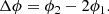 (2)
(2)
The waveform shape is governed by the amplitude ratio A2/A1 and the relative phase Δϕ. Appendix C shows qualitatively when considering the light curve flux that:
 (3)
(3)
 (4)
(4)
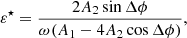
This phase difference Δϕ provides a robust, model-independent diagnostic: A population of stars showing Δϕ ≈ ±π is consistent with the binary scenario, while Δϕ ≈ 0 is naturally explained by oscillatory dipole modes viewed at high inclination. We note that Δϕ ≈ ±π would only be consistent with an oscillatory dipole if there is a more complex non-linear relationship between temperature and brightness than the simple blackbody function used here. In practice, Δϕ is stable to OGLE sampling and noise for the harmonic-selected sample (typical uncertainties of order ≤10°). We note that performing this analysis on stellar magnitude, rather than flux reverses this phase condition. All measurements in this work are based on normalised flux light curves (not magnitudes).
2.2. Harmonic visibility across parameter space
To identify when thermal dipole modes produce observable harmonics, we simulated light curves across a grid of different dipole inclination angles (θobs) temperature amplitudes (δTeff) and observed wavelength (λobs), scaled by the blackbody peak λBB, peak from Wien’s law. A harmonic is deemed ‘observable’ when the secondary peak amplitude exceeds 5% of the primary, which is measured directly in the time domain from peak spacings and heights. This approach avoids false positives from sharp asymmetric peaks that contaminate power spectral methods at high λBB, peak/λobs ratios. The specific threshold was chosen because in OGLE light curves a 5% harmonic amplitude typically exceeds the photometric noise floor, even for faint LMC giants. Figure 2 shows example light curves at high versus low inclination. Figure 3 maps the parameter space where LSP harmonics are expected to be observable. This observability fundamentally depends on the effective temperature of the star (parameterised as the wavelength λBB, peak of the blackbody’s peak from Wien’s law), the observation wavelength (λobs), the inclination of the dipole and its amplitude δT. Peak observability is found around λBB, peak/λobs ∼ 3, and no harmonic signature is found for inclinations below 48 degrees. For a typical red giant with Teff ∼ 3500 K, the blackbody peak occurs near λpeak ∼ 0.83 μm, implying increased sensitivity to temperature perturbations at shorter visible wavelengths. While this suggests larger fractional variations in the V-band compared to I, the OGLE V-band light curves are more sparsely sampled, limiting their suitability for harmonic phase analysis. The model also predicts phase-dependent colour variations, with larger amplitudes at shorter wavelengths leading to periodic differential colour changes. In addition, the dipole mode is expected to produce radial velocity variations through associated surface flows, including a radial component (Saio et al. 2015; Takayama & Ita 2020). These provide additional diagnostics for future study.
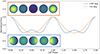 |
Fig. 2. Example of an inclined vs face-on oscillatory convective dipole causing a secondary maxima in the light curve, therefore producing a harmonic signal. |
2.3. Assumption of no rotation
In the simulations presented above, we assumed the thermal dipole pattern remains fixed in the co-rotating frame of the star and that stellar rotation is negligible over the timescale of the LSP. This implies that the dipole oscillation maintains a constant orientation relative to the observer, modulating the observed flux purely through geometric projection and thermal contrast. This assumption is justified if the stellar rotation period is much longer than the LSP, which has been shown to often be the case in the stellar envelope (Olivier & Wood 2003; Li et al. 2024). However, in more rapidly rotating stars, the dipole axis may precess or sweep across the line of sight, modifying the harmonic content and introducing phase shifts in the light curve. We note that the harmonic observability maps shown in Figure 3 reflect only the static, non-rotating case. More discussion on this is presented in Appendix F.
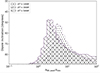 |
Fig. 3. Shaded regions indicate combinations of dipole amplitude, viewing inclination, and λBB, peak/λobs where harmonic features appear in synthetic light curves. |
3. Observational examples
3.1. Harmonic filtering and sample selection
We began with the OGLE catalogue of LSP variables and identified stars whose two strongest periods (P1, P2) correspond to sequence D and the D1/2 ridge. This produced two complementary cases: (1) one case where the period with the strongest amplitude (P1) is on sequence D, and the period corresponding to the second strongest amplitude (P2) is at roughly half of P1 (i.e. on sequence D1/2), and (2) another where the period with the strongest amplitude is on sequence D1/2 and the period corresponding to the second strongest amplitude is at twice the period (i.e. on sequence D). We considered a ∼10% uncertainty on the allowable ratio of P2/P1 roughly consistent with the full width at half maximum found in the mean Lomb-Scargle Periodograms (Figure A.1). Formally this gives us the following criteria:
![Mathematical equation: $$ \begin{aligned} \mathrm{(set~1) :}~P_1&\in D, \quad \frac{P_2}{P_1} \in \left[\frac{1}{2.2},\,\frac{1}{1.8}\right],\\ \mathrm{(set~2) :}~P_1&\in D_{1/2},\quad \frac{P_2}{P_1} \in [1.8,\,2.2]. \end{aligned} $$](/articles/aa/full_html/2026/05/aa59620-26/aa59620-26-eq5.gif)
An I-band amplitude threshold (Iamp1 ≥ 0.05 mag) was also applied to ensure samples have a reasonable signal-to-noise ratio (SNR). For each selected star we analysed the OGLE I-band light curve (converted to normalised flux). We fit each OGLE light curve with a multi-sinusoid Fourier model using an iterative frequency-selection procedure. Details are outlined in Appendix D. Histograms of Δϕ for each subset are shown in Fig. 4.
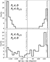 |
Fig. 4. Distribution of relative phase differences Δϕ = ϕ2 − 2ϕ1 for Set 1 (n = 125, top) and Set 2 (n = 124, bottom). The peak at Δϕ ≈ 0° indicates secondary maxima (dipole-like), while ±180° indicates secondary minima (binary-like). |
3.2. Discussion: Harmonic phase differences and morphology
Set 1 with the strongest period on sequence D has a distribution of Δϕ that strongly peaks around 180 degrees, and contains no samples with Δϕ ∼ 0, indicating secondary minima consistent with a binary scenario in a circular orbit. However, when considering set 2 (isolating samples with the strongest period on sequence D1/2), we found a significantly different distribution that peaks below 180 degrees, and contains ∼3% of secondary maxima with Δϕ ∼ 0. An example light curve with Δϕ ∼ 0 showing the fitted Fourier model and isolated fundamental and harmonic components is shown in Figure 5. A second example is shown in Appendix G, demonstrating that the secondary-maximum morphology is not unique to a single star. These examples are candidate oscillatory dipoles viewed at high inclination, as predicted by the harmonic content. To verify that secondary maxima in the harmonic-selected sample are physical, we tested the robustness of the relative phase Δϕ to photometric noise and the irregular OGLE cadence. Monte Carlo injections of synthetic binary-like light curves (Δϕ = π) demonstrate that noise-driven phase inversions of ∼180° are negligible at the SNR levels of our sample (Appendix E). We also considered contamination from ellipsoidal variables (sequence E), which overlap the harmonic ridge D1/2. These generally produce near-symmetric light curves with little power in the first harmonic. Such systems are typically filtered out by our harmonic-selection criteria. In the minority of cases where ellipsoidal modulation produces asymmetric light curves with detectable harmonic content, the resulting phase difference remains close to Δϕ ≈ π, reinforcing the population of secondary minima rather than mimicking the distinctive secondary maxima (Δϕ ≈ 0). Considering a ∼3000 K primary observed in the OGLE I-band (0.8 μm), λBB, peak/λobs ∼ 1.2. From Fig. 3, the probability that a randomly oriented dipole exceeds the minimum inclination im for observability is P(O) = cos im. For δT ∼ 100 K (Takayama & Ita 2020), we estimated im ≈ 88° (P ≈ 0.03), and for δT = 500 K, im ≈ 81° (P ≈ 0.15). When using a ±10° bin around Δϕ = 0, set 2 contains a fraction ≃0.03, which is broadly consistent with the geometric expectation for δT ∼ 100 K, where harmonics occur only at high inclinations. This comparison is qualitative, as the sample is harmonic-selected and SNR-limited, whereas the inclination estimate applies to the full sequence D population. The concentration near Δϕ ∼ ±180° further indicates that set 2 is a mixed sample with a significant binary contribution.
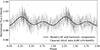 |
Fig. 5. Folded I-band light curve of OGLE-LMC-LPV-64405 filtered for the LSP signal and first harmonic. Grey points show cleaned OGLE data repeated over two cycles. The black curve is the model fit exhibiting a secondary maximum, consistent with an inclined dipole. |
We highlight the concern of Saio et al. (2015) that when adopting a mixing length parameter that is consistent with measured effective temperatures of the red-giant sequences of the LMC, the oscillatory convective modes predicted periods too short by a factor of two, i.e. exactly where we see the sequence D1/2. It is also here where we observed a broadly consistent fraction of secondary maxima predicted simply by the dipole geometry in inclined systems. However, the use of a single mixing-length parameter to characterise convection throughout the stellar envelope may be overly restrictive.
4. Conclusion
The relative phase (Δϕ) of light curve harmonics serves as a powerful diagnostic to distinguish between LSP physical origins. While binary systems produce characteristic secondary minima (Δϕ ≈ ±180°), we have shown that inclined oscillatory convective dipole modes naturally generate secondary maxima (Δϕ ≈ 0). Our analysis of the OGLE-III LMC catalogue reveals that while binarity explains the majority of harmonic-rich LSPs, a statistically non-negligible subset exhibits the secondary-maximum morphology predicted by dipole models. These findings suggest that LSPs represent a mixed population driven by both binary companions and convective oscillations. Future work must now focus on modelling observational selection effects to determine the true relative fraction of each mechanism across the red-giant population.
Acknowledgments
This work was supported through an Australian Government Research Training Program Scholarship. Special thanks to K.A.E and the SSO.
References
- Ceillier, T., Tayar, J., Mathur, S., et al. 2017, A&A, 605, A111 [NASA ADS] [CrossRef] [EDP Sciences] [Google Scholar]
- Claret, A., & Bloemen, S. 2011, A&A, 529, A75 [NASA ADS] [CrossRef] [EDP Sciences] [Google Scholar]
- Cole, A. A., Tolstoy, E., Gallagher, J. S., III, et al. 2005, AJ, 129, 1465 [NASA ADS] [CrossRef] [Google Scholar]
- Courtney-Barrer, B., Haubois, X., Wood, P., et al. 2026, A&A, 705, A187 [NASA ADS] [CrossRef] [EDP Sciences] [Google Scholar]
- Decin, L., Vermeulen, O., Esseldeurs, M., et al. 2025, A&A, 703, L23 [NASA ADS] [CrossRef] [EDP Sciences] [Google Scholar]
- Fulton, B. J., Rosenthal, L. J., Hirsch, L. A., et al. 2021, ApJS, 255, 14 [NASA ADS] [CrossRef] [Google Scholar]
- González Hernández, J. I., & Bonifacio, P. 2009, A&A, 497, 497 [Google Scholar]
- Gordon, K. D., Clayton, G. C., Misselt, K. A., et al. 2003, ApJ, 594, 279 [NASA ADS] [CrossRef] [Google Scholar]
- Hocdé, V., Smolec, R., Moskalik, P., et al. 2023, A&A, 671, A157 [NASA ADS] [CrossRef] [EDP Sciences] [Google Scholar]
- Li, G., Deheuvels, S., & Ballot, J. 2024, A&A, 688, A184 [NASA ADS] [CrossRef] [EDP Sciences] [Google Scholar]
- Nicholls, C. P., Wood, P. R., Cioni, M. R. L., et al. 2009, MNRAS, 399, 2063 [CrossRef] [Google Scholar]
- Nicholls, C. P., Wood, P. R., & Cioni, M.-R. L. 2010, MNRAS, 405, 1770 [NASA ADS] [Google Scholar]
- Olivier, E. A., & Wood, P. R. 2003, ApJ, 584, 1035 [Google Scholar]
- Pawlak, M. 2021, A&A, 649, A110 [NASA ADS] [CrossRef] [EDP Sciences] [Google Scholar]
- Pawlak, M., Soszyński, I., Pietrukowicz, P., et al. 2014, Acta Astron., 64, 293 [NASA ADS] [Google Scholar]
- Saio, H., Wood, P. R., Takayama, M., et al. 2015, MNRAS, 452, 3863 [NASA ADS] [CrossRef] [Google Scholar]
- Soszynski, I., Udalski, A., Kubiak, M., et al. 2004, Acta Astron., 54, 347 [Google Scholar]
- Soszyński, I., Olechowska, A., Ratajczak, M., et al. 2021, ApJ, 911, L22 [CrossRef] [Google Scholar]
- Takayama, M., & Ita, Y. 2020, MNRAS, 492, 1348 [NASA ADS] [CrossRef] [Google Scholar]
- Trabucchi, M., Wood, P. R., Montalbán, J., et al. 2019, MNRAS, 482, 929 [Google Scholar]
- Wood, P. R., Alcock, C., Allsman, R. A., et al. 1999, in Asymptotic Giant Branch Stars, eds. T. Le Bertre, A. Lebre, & C. Waelkens, 191, 151 [Google Scholar]
- Wood, P. R., Olivier, E. A., & Kawaler, S. D. 2004, ApJ, 604, 800 [Google Scholar]
Appendix A: Lomb-Scargle periodogram of sequence D and D1/2
Figure A.1 shows period normalised Lomb-Scargle Periodograms for the sequence D and D1/2 samples.
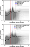 |
Fig. A.1. Lomb-Scargle Periodograms for I-band light curves from the OGLE-III LMC catalogue, with time series normalised to the classified primary period, of sequence D (left) and sequence D1/2 (right) LMC stars. |
Appendix B: Oscillatory convective mode modelling
B.1. Thermal dipole model
We model the star’s temperature field as an oscillatory dipole (Takayama & Ita 2020), represented by a low-order spherical harmonic:
![Mathematical equation: $$ \begin{aligned} T_{\text{ eff,local}} = T_{\text{ eff}} + \delta T_{\text{ eff}} \, \text{ Re}\left[ \frac{Y_l^m(\theta , \phi )}{\max \text{ Re}(Y_l^m)} e^{i(2\pi \nu t + \psi _T)} \right], \end{aligned} $$](/articles/aa/full_html/2026/05/aa59620-26/aa59620-26-eq6.gif) (B.1)
(B.1)
where Teff is the mean stellar effective temperature, δTeff is the dipole amplitude, and ψT is the phase. The spherical harmonic Ylm(θ, ϕ) is normalised to unit peak amplitude and modulates the local surface temperature over time (Takayama & Ita 2020).
B.2. Effective temperature estimates for LMC stars
To initialise realistic simulations, we estimate effective temperatures for LMC stars using V and Ks photometry from OGLE, corrected for extinction with AV = 0.3 and AKs = 0.114 × AV (Gordon et al. 2003):
 (B.2)
(B.2)
We then apply the empirical calibration from González Hernández & Bonifacio (2009):
![Mathematical equation: $$ \begin{aligned} \theta _{\mathrm{eff} }&= b_0 + b_1 X + b_2 X^2 + b_3 X\,[\mathrm{Fe/H} ] + b_4\,[\mathrm{Fe/H} ] + b_5\,[\mathrm{Fe/H} ]^2, \end{aligned} $$](/articles/aa/full_html/2026/05/aa59620-26/aa59620-26-eq8.gif) (B.3)
(B.3)
 (B.4)
(B.4)
with X = (V − Ks)0 and [Fe/H] = −0.19, typical of LMC giants (Hocdé et al. 2023).
B.3. Limb darkening
To account for disc-integrated flux effects, we include linear limb darkening using coefficients from Claret & Bloemen (2011), matched to Teff, log g ∼ 0, and [Fe/H] = −0.4 typical of AGB stars (Cole et al. 2005):
 (B.5)
(B.5)
where μ = cos θ is the angle to the line of sight and u is the band-specific limb-darkening coefficient.
B.4. Projection and observables
The temperature-modulated, limb-darkened intensity map is rotated into the observer’s frame via:
 (B.6)
(B.6)
followed by projection onto the 2D plane:
 (B.7)
(B.7)
and with the total observed flux computed over the visible hemisphere (μ > 0):
 (B.8)
(B.8)
The resulting synthetic light curves include geometric modulation, temperature asymmetry, and disc integration.
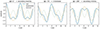 |
Fig. B.1. Example waveforms showing the sum of a fundamental signal and its first harmonic for a fixed amplitude ratio of 0.5. The three panels correspond to relative phase offsets of 0, 60, and 180°, illustrating how changes in the phase relationship between the two components produce distinct waveform shapes–ranging from profiles with secondary maxima to asymmetric peaks and secondary minima. |
Appendix C: Harmonic phase relation for secondary minima vs maxima
Beginning with the general waveform:
 (C.1)
(C.1)
The waveform shape is governed by the amplitude ratio A2/A1 and the relative phase Δϕ. To characterise the nature of the secondary extremum, consider the neighbourhood of  , where the fundamental alone has a minimum. Expanding to second order, the derivatives are:
 (C.2)
(C.2)
 (C.3)
(C.3)
Using approximations near t = π/ω, we find:
 (C.4)
(C.4)
The quantity ε★ represents the first-order shift in the location of the extremum induced by the harmonic term. Evaluating the curvature at t = π/ω + ε★ ensures that the classification as a minimum or maximum is performed at the true stationary point of the combined waveform. The curvature at this stationary point is:
 (C.5)
(C.5)
Therefore:
 (C.6)
(C.6)
Evaluating the signal directly at  gives:
 (C.7)
(C.7)
Thus, cos Δϕ > 0 lifts the minima (tending towards a secondary maximum), while cosΔϕ < 0 deepens it (enhancing the minimum). In qualitative terms:
 (C.8)
(C.8)
 (C.9)
(C.9)
Higher-order harmonics (n > 2) behave analogously, with ϕn − nϕ1 controlling the location and type of additional extrema. A subtle, but important point is considering when the light curve is in units of magnitude (Xm), as in the OGLE catalogue, i.e.:
 (C.10)
Accordingly the signs are reversed and we get:
 (C.11)
 (C.12)
Appendix D: Fourier fitting of OGLE light curves
After selecting the highest peak (excluding a small neighbourhood around previously selected frequencies), we refit all selected components simultaneously using weighted linear least squares with weights wi = 1/σi2, where σi is the reported photometric uncertainty of datum yi. We solve for an offset and sine-cosine coefficient pairs at each frequency. A newly added frequency is retained only if the Bayesian Information Criterion (BIC) improves, adopting BIC = χ2 + klnN, where χ2 is the standard chi-square statistic, N is the number of data points used in the fit and k = 1 + 2m for m fitted frequencies. The iteration terminates once the BIC no longer decreases. For each accepted component, the sine-cosine coefficients are converted to an amplitude and phase under a cosine convention, allowing evaluation of the phase relation Δϕ between a dominant frequency and a near-harmonic counterpart.
Appendix E: Robustness of harmonic phase measurements
To assess whether the secondary maxima identified in the harmonic-selected subset of sequence D stars could arise from noise-induced misclassification, we performed Monte Carlo simulations of synthetic light curves with known harmonic structure. Each simulation consisted of a signal of the form described in C.1 sampled either at the observed OGLE cadence or using a simplified seasonal cadence designed to reproduce the sparse and irregular sampling typical of the survey. Gaussian photometric noise was added at levels matched to the SNR of the harmonic component in the real sample. For each realisation, the fundamental and first harmonic were fit at the known frequencies using a linear least-squares model, and the relative phase Δϕ = ϕ2 − 2ϕ1 was recovered. This procedure intentionally conditions on the presence of significant power at both the fundamental and harmonic periods, mirroring the harmonic-selection step applied to the OGLE-III data, and isolates the effect of noise and cadence on the recovered phase alone. The simulations therefore do not test the detectability of harmonic power or the reliability of period identification, but specifically address whether noise can cause a true secondary minimum (Δϕ = π) to be misidentified as a secondary maximum (Δϕ = 0).
Across 2 × 10⁴ realisations, the recovered Δϕ distribution remains tightly clustered around the true value even with poor cadence (down to tens of days per year), with no statistically significant population of phase flips by ∼180° at the SNR levels of the observed sample. The recovered phase scatter is well described by a width of order ∼10°, supporting the use of a ±10° bins in the histograms of the main analysis. Example simulated light curves and the corresponding Δϕ distributions are shown in Figure E.1.
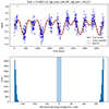 |
Fig. E.1. Monte Carlo test of harmonic phase recovery for a synthetic light curve with a true secondary minimum (Δϕ = 180°). Top: Example realisation showing the noiseless model (black dashed), noisy sampled data with seasonal cadence (blue points), and the best-fitting two-harmonic model recovered at the known fundamental and harmonic frequencies (red). Bottom: Distribution of recovered relative phases Δϕ = ϕ2 − 2ϕ1 over 2 × 10⁴ Monte Carlo realisations. The shaded region indicates a ±10° window around Δϕ = 0, corresponding to the secondary maxima regime. No significant population of noise-driven phase flips from Δϕ = 180° to Δϕ ≈ 0 is observed, demonstrating that such misclassification is negligible at the signal-to-noise levels considered. |
Appendix F: Discussion on rotation
Our models assumption of non-rotation is generally justified for our red-giant sample. However, there are certainly cases where the LSP could be comparable to the rotation period, especially in binary systems. In practice this produces a scatter in Δϕ, broadening the histogram and occasionally shifting individual stars towards intermediate values. Asteroseismic analysis using Kepler data by Ceillier et al. (2017) found that only ∼2% of red giants with solar-like oscillations exhibit detectable surface rotation periods. More recently, Li et al. (2024) conducted a large survey of 2,495 RGB stars and measured core and surface rotation using rotational splittings of mixed modes. Of the detectable periods they reported periods mostly in the 200 - to few-thousand-day range, with core-to-envelope rotation ratios peaking near 20 for RGB stars, indicating significant differential rotation. In this context, the width of our Δϕ distribution becomes an important diagnostic: stars near Δϕ ≈ 0° likely represent dipoles in nearly non-rotating or slowly rotating envelopes. Stars with larger deviations may reflect modest rotation-induced phase drifts and/or frequency chirps. Simple geometric models could be included to characterise the harmonic precession under a dipole hypothesis. There remains an important uncertainty concerning the rotational coupling of the oscillatory convective dipole, and whether this large-scale convective asymmetry is anchored in the more rapidly rotating core, the slowly rotating envelope, or a distinct intermediate shell.
Appendix G: Additional example of secondary maxima
Figure G.1 shows a second example from the Δϕ ∼ 0 subset. The folded OGLE I-band light curve exhibits a clear secondary maximum consistent with the inclined oscillatory convective dipole interpretation described in the main text. This demonstrates that the morphology shown in Figure 5 is not unique to a single object.
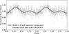 |
Fig. G.1. Folded OGLE I-band light curve of OGLE-LMC-LPV-29787. An additional example where the fitted sequence D and harmonic component shows a clear secondary maxima corresponding to Δϕ ∼ 0 (dipole mode). |
All Figures
|
Fig. 1. Sequence D (red) in the PL diagram along with a sub-sequence at close to the second harmonic of sequence D which we highlight in yellow and label sequence D1/2. This ridge largely overlaps with the classical sequence E associated with ellipsoidal binaries, but is highlighted to illustrate the presence of harmonic structure in sequence D stars, and to motivate the harmonic-filtered selection used in Section 3.1. |
| In the text | |
|
Fig. 2. Example of an inclined vs face-on oscillatory convective dipole causing a secondary maxima in the light curve, therefore producing a harmonic signal. |
| In the text | |
|
Fig. 3. Shaded regions indicate combinations of dipole amplitude, viewing inclination, and λBB, peak/λobs where harmonic features appear in synthetic light curves. |
| In the text | |
|
Fig. 4. Distribution of relative phase differences Δϕ = ϕ2 − 2ϕ1 for Set 1 (n = 125, top) and Set 2 (n = 124, bottom). The peak at Δϕ ≈ 0° indicates secondary maxima (dipole-like), while ±180° indicates secondary minima (binary-like). |
| In the text | |
|
Fig. 5. Folded I-band light curve of OGLE-LMC-LPV-64405 filtered for the LSP signal and first harmonic. Grey points show cleaned OGLE data repeated over two cycles. The black curve is the model fit exhibiting a secondary maximum, consistent with an inclined dipole. |
| In the text | |
|
Fig. A.1. Lomb-Scargle Periodograms for I-band light curves from the OGLE-III LMC catalogue, with time series normalised to the classified primary period, of sequence D (left) and sequence D1/2 (right) LMC stars. |
| In the text | |
|
Fig. B.1. Example waveforms showing the sum of a fundamental signal and its first harmonic for a fixed amplitude ratio of 0.5. The three panels correspond to relative phase offsets of 0, 60, and 180°, illustrating how changes in the phase relationship between the two components produce distinct waveform shapes–ranging from profiles with secondary maxima to asymmetric peaks and secondary minima. |
| In the text | |
|
Fig. E.1. Monte Carlo test of harmonic phase recovery for a synthetic light curve with a true secondary minimum (Δϕ = 180°). Top: Example realisation showing the noiseless model (black dashed), noisy sampled data with seasonal cadence (blue points), and the best-fitting two-harmonic model recovered at the known fundamental and harmonic frequencies (red). Bottom: Distribution of recovered relative phases Δϕ = ϕ2 − 2ϕ1 over 2 × 10⁴ Monte Carlo realisations. The shaded region indicates a ±10° window around Δϕ = 0, corresponding to the secondary maxima regime. No significant population of noise-driven phase flips from Δϕ = 180° to Δϕ ≈ 0 is observed, demonstrating that such misclassification is negligible at the signal-to-noise levels considered. |
| In the text | |
|
Fig. G.1. Folded OGLE I-band light curve of OGLE-LMC-LPV-29787. An additional example where the fitted sequence D and harmonic component shows a clear secondary maxima corresponding to Δϕ ∼ 0 (dipole mode). |
| In the text | |
Current usage metrics show cumulative count of Article Views (full-text article views including HTML views, PDF and ePub downloads, according to the available data) and Abstracts Views on Vision4Press platform.
Data correspond to usage on the plateform after 2015. The current usage metrics is available 48-96 hours after online publication and is updated daily on week days.
Initial download of the metrics may take a while.