| Issue |
A&A
Volume 682, February 2024
|
|
|---|---|---|
| Article Number | A88 | |
| Number of page(s) | 10 | |
| Section | Catalogs and data | |
| DOI | https://doi.org/10.1051/0004-6361/202346163 | |
| Published online | 07 February 2024 | |
Investigating the long secondary period phenomenon with the ASAS-SN and Gaia data★
1
Astronomical Observatory, Jagiellonian University,
ul. Orla 171,
30-244
Kraków,
Poland
2
Lund Observatory, Division of Astrophysics, Department of Physics, Lund University,
Box 43,
221 00
Lund,
Sweden
e-mail: This email address is being protected from spambots. You need JavaScript enabled to view it.
3
Dipartimento di Fisica e Astronomia Galileo Galilei, Università degli studi di Padova,
Vicolo dell’Osservatorio 3,
35122
Padova,
Italy
4
Department of Astronomy, University of Geneva,
Chemin Pegasi 51,
1290
Versoix,
Switzerland
5
Department of Astronomy, University of Geneva,
Chemin d’Ecogia 16,
1290
Versoix,
Switzerland
Received:
16
February
2023
Accepted:
14
November
2023
Abstract
Aims. The aim of this work is to create a complete list of sources exhibiting a long secondary period (LSP) in the ASAS-SN catalog of variable stars, and analyze the properties of this sample compared to other long period variables without an LSP.
Methods. We used the period-amplitude diagram to identify the 55 572 stars showing an LSP, corresponding to 27% of the pulsating red giants in the catalog. We used astrometric data from Gaia DR3 and spectroscopic data provided by the APOGEE, GALAH, and RAVE surveys to investigate the statistical properties of the sample.
Results. We find that stars displaying an LSP have a spatial distribution that is more dispersed than that of the non-LSP giants, suggesting that they belong to an older population. Spectroscopically derived ages seem to confirm this. The stars with an LSP also appear to be different in terms of the C/O ratio from their non-LSP counterparts.
Key words: stars: AGB and post-AGB / pulsars: general / stars: variables: general
The catalogue is available at the CDS via anonymous ftp to cdsarc.cds.unistra.fr (130.79.128.5) or via https://cdsarc.cds.unistra.fr/viz-bin/cat/J/A+A/682/A88
© The Authors 2024
 Open Access article, published by EDP Sciences, under the terms of the Creative Commons Attribution License (https://creativecommons.org/licenses/by/4.0), which permits unrestricted use, distribution, and reproduction in any medium, provided the original work is properly cited.
This article is published in open access under the Subscribe to Open model. This email address is being protected from spambots. You need JavaScript enabled to view it. to support open access publication.
1 Introduction
The long secondary period (LSP) phenomenon is observed in a significant fraction of long period variables (LPVs). It is an additional source of periodic variability that exists alongside the primary, pulsational variability but cannot be explained by radial pulsation. Despite the fact that the phenomenon has been known for along time (O’Connell 1933; Payne-Gaposchkin 1954; Houk 1963), its origin still lacks a full explanation. A number of hypotheses have been put forward to explain the origin of the LSP. The two most common include binarity (Wood et al. 1999; Soszyński 2007; Soszyński and Udalski 2014; Soszyński et al. 2021) and non-radial pulsation (Wood 2000a,b; Hinkle et al. 2002; Wood et al. 2004; Saio et al. 2015).
Long secondary period stars were spectroscopically observed by Nicholls et al. (2009), who measured their radial velocities in order to verify the binary hypothesis, concluding that the classical binary with a stellar companion can be ruled out. However, neither the low-mass companion scenario nor the one involving non-radial pulsations could be excluded. An analysis of the spectroscopic properties of a small sample of LSPs was carried out by Pawlak et al. (2019), who noted some possible differences in basic spectroscopic parameters including log ɡ, the effective temperature, and metallicity. A similar study was done by Jayasinghe et al. (2021), who concluded that no significant difference can be seen.
In this paper, we use the All Sky Automated Survey for Supernovae (Shappee et al. 2014; Jayasinghe et al. 2018, ASAS-SN) catalog of LPVs combined with Gaia Data Release 3 (Gaia Collaboration 2021, 2023, DR3) to identify a complete, all-sky sample of LSPs and study their properties compared to the non-LSP red giants. We further extend our analysis using spectroscopic data provided by the APOGEE (Majewski et al. 2017), GALAH (De Silva et al. 2015), and RAVE (Steinmetz et al. 2006) surveys.
The structure of the paper is as follows: Sect. 2 describes the data set we used and Sect. 3 presents the analysis of the spatial distribution, kinematics, and spectroscopic properties of the sample. We discuss the results in Sect. 4.
2 Data
For the purpose of this study we used the ASAS-SN Catalog of Variable Stars containing 194 840 LPVs (Jayasinghe et al. 2018, 2019a,b). The sample includes both semi-regular as well as OGLE small-amplitude red giant (OSARG) type variables. We crossmatched this catalog with the Gaia DR3 catalog (Gaia Collaboration 2021), obtaining 186 583 matches. This was our base sample, which we used for further analysis.
The dominant variability period is given in the ASAS-SN catalog. However, since the LSP can appear not only as the strongest but also as the second or further period, we decided to run an independent period search to identify the three strongest periods for each of the objects. For that purpose, we use the Lomb–Scargle method implemented in the VAROOLS package (Hartman & Bakos 2016).
The criterion we used to select LSP stars was A < 1.6 log(P) − 3.7, where P is the strongest period in days and A is the V-band peak-to-peak amplitude in magnitudes. The selection criterion we propose was empirically chosen with a trial and error approach to optimally separate the LSP stars from long-period pulsators. Figure 1 illustrates the selection method. We first checked the period with the strongest S/N and, if it did not meet the LSP criterion, we checked the second and third periods.
The LSP stars have traditionally been selected based on their location on the period-lumonosity diagram (PLD). This approach has certain limitations related to the fact that it requires accurate distances and mean NIR or MIR photometry. In the absence of accurate distance determinations, the sequences C (formed by the fundamental mode pulsators) and D (formed by the LSP stars) tend to overlap, making the distinction between Mira periods and LSPs rather difficult. Interstellar extinction further complicates the issue.
The method we propose is meant to achieve the same result, avoiding the aforementioned limitations. For that purpose, period-amplitude selection can be used as an effective tracer of sequence D (Trabucchi et al. 2017; Lebzelter et al. 2019).
To test the reliability of our method, we used the OGLE catalogue of LPV stars in the Large Magellanic Cloud (Soszyński 2007), where the period-luminosity sequences are well defined. We selected the LSP candidates using the period-amplitude criterion defined above and placed them on the PLD (Fig. 2). The vast majority of the selected candidates lie on sequence D, with very few outliers, showing that the period-amplitude criterion is an effective way of selecting LSP stars. It also allows us to separate the LSP stars in sequence D from the ellipsoidal binaries at the tip of sequence E (the clump of stars to the left with periods between 100 and 200 days form the LSP sequence).
We note that our ability to detect the LSP is dependent on the magnitude of the star, as the root mean square (RMS) of ASAS-SN photometry gets higher for fainter objects. As shown in Jayasinghe et al. (2019b), the typical RMS remains at the level of 0.01 mag up to V = 13 mag and then rises steadily to about 0.1 mag at V = 17 mag. Therefore, to avoid spurious detection, we introduced a cut on the amplitude of the faint stars, defined as A > 0.036 ⋅ V − 0.458. In the whole sample, we identified 32 983 stars where LSP is the strongest period and 22 831 where LSP is the second or third strongest period.
In order to verify the performance of the selection method proposed and further analyze the period-luminosity relations, we computed the Wesenheit reddening-free indexes, as is defined in Lebzelter et al. (2019), using both Gaia and 2MASS photometry and correcting it for the distance module based on Gaia parallaxes. We discarded the stars with negative parallaxes. The formulas for Gaia (Wrp) and 2MASS (Wjk) indexes are given by
 (1)
(1)
 (2)
(2)
where ϖ is the Gaia parallax, Gbp and Grp are Gaia blue and red photometer magnitudes, and J and K are 2MASS infrared magnitudes. In Fig. 3, we display the (PLD) of stars in which the LSP is dominant, showing both the LSP (top panel) and the pulsation periods (bottom panel). The same diagram is shown in Fig. 4 for the stars whose strongest period is not an LSP, but rather due to pulsation. The first thing we can observe is that the periods that we flagged as LSP, based on the period-amplitude, are actually located in sequence D, showing that our selection method is consistent with the traditionally used method based on the location on the PLD. We note that the two types of star, shown in Figs. 3 and 4, display clearly different distributions. When the LSP is weaker than pulsation periods, the latter tend to be shorter than 100 days, and populate sequences A and B (for the sequence labels we adopt the same nomenclature as Wood 2015). Conversely, the pulsation periods of stars dominated by the LSP can be longer than 100 days and reach the area associated with sequences C′, F, and C.
The comparison of the LSP to the pulsation period ratio (Fig. 5) reveals the likely cause of the difference mentioned above. For the objects with an LSP discovered as the second or third period, the PLSP/PPULS ratio does not show any preferential value. However, for stars where the LSP is the strongest period, the distribution has a very prominent peak at PLSP/PPULS = 2. It strongly suggests that in these cases the second period is not an actual pulsational period but a harmonic of the LSP. Therefore, for the objects where the second period is longer than 100 days, we took the third period and adopted it as PPULS. We also identified 241 where the putative LSP turned out to be an alias of the high-amplitude, long pulsational period. We removed those from our LSP list. The sample corrected this way is shown in Fig. 6.
We are making the list of identified LSPs, together with all three identified periods, including their pulsational and long periods, publicly available in an electronic format at CDS.
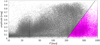 |
Fig. 1 Selection of the LSP stars based on the location on the period-amplitude diagram. Periods selected as LSPs are marked in magenta, while other LPVs are marked in gray. The cutoff criterion is A < 1.6 log(P) − 3.7, and is marked with a dashed black line. |
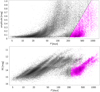 |
Fig. 2 Verification of the selection criterion using the OGLE LMC sample (Soszyński et al. 2007). The period-amplitude cutoff marked with dashed line is the same as in Fig. 1. The objects selected with the cutoff (upper panel) are placed on the PL diagram (lower panel). For the PL diagram, we use the redenig-free Wesenheit index WI = V − 1.55(V − I). |
3 Analysis
3.1 Comparison sample
We further examined our sample of LSP stars in order to assess if they stand out from other LPVs in terms of population effects or spectroscopic properties. It is known that the appearance of LSPs is related to the evolutionary status of the star (Trabucchi et al. 2017; Pawlak 2021). The least evolved LPVs do not show an LSP at all, and the more evolved on the RGB or AGB the star gets, the more likely it is to show an LSP. This effect needs to be taken into account when comparing the LSP and non-LSP samples, as it will obviously bias the analysis. Therefore, to make a proper comparison, we need to define a control sample of non-LSP stars that are approximately at the same evolutionary point as the LSP sample stars. For that purpose, we used the log(P) versus WJK plane, where for LSP stars we used the pulsational period as P. We removed the stars with negative parallaxes and those with ϖ < σϖ, where σϖ is the Gaia parallax uncertainty. We defined X and Y coordinates by normalizing both the log(P) and WJK range to [0:1]. This way, we obtained a rectangular XY coordinates grid. Then, we took each LSP star and used the simple 2D Cartesian metric to find the nearest non-LSP star. This way we ended up with an equally numerous control sample of non-LSP stars that have approximately the same distribution in the PL diagram as the sample of LSP-dominated stars. In other words, we obtained a control sample of stars that could have shown LSP but do not.
To make sure that the construction of the control sample does not introduce any additional bias, we constructed another, randomized control sample. In this case, instead of using the exact WJK, we took a value randomly drawn from the ![Mathematical equation: $\left[ {{W_{{\rm{JK}}}} - {\sigma _{{W_{{\rm{JK}}}}}},{W_{{\rm{JK}}}} + {\sigma _{{W_{{\rm{JK}}}}}}} \right]$](/articles/aa/full_html/2024/02/aa46163-23/aa46163-23-eq3.png) interval and used it to compute the Y coordinate. Since we considered the uncertainty of P to be negligible, we left the X coordinate unchanged. We obtained the randomized coordinates of each of the LSP stars and then selected a new nearest non-LSP star. The additional, randomized control sample obtained this way can be used for the purpose of performing quality checks. In the following, the sets constructed with this approach are indicated as the control sample and the randomized control sample, while we refer to the sets of stars that show or do not show an LSP as the LSP sample and the non-LSP sample, respectively.
interval and used it to compute the Y coordinate. Since we considered the uncertainty of P to be negligible, we left the X coordinate unchanged. We obtained the randomized coordinates of each of the LSP stars and then selected a new nearest non-LSP star. The additional, randomized control sample obtained this way can be used for the purpose of performing quality checks. In the following, the sets constructed with this approach are indicated as the control sample and the randomized control sample, while we refer to the sets of stars that show or do not show an LSP as the LSP sample and the non-LSP sample, respectively.
3.2 Spatial distribution and dynamical properties
We compared the LSP sample to both the whole non-LSP sample and the control sample. First, we examined their sky spatial distribution, which is illustrated in Fig. 7. We note that the LSP sample seems to be more concentrated around the Galactic bulge and has a larger dispersion along the Galactic latitude (b). To check this, we compared the distribution of the samples in b. This is illustrated in Fig. 8. The distribution of the LSP sample shows a statistically significant difference and indeed appears to be more dispersed in b, especially on the negative side of the distribution. To complete the spatial distribution picture, we also compared the distribution in the Galactic longitude, l (Fig. 9), and in the Gaia parallaxes, ϖ, which is shown in Fig. 10, toward both the center and anti-center of the Galaxy. Again, we see a significant difference between LSP and non-LSP stars.
Next, we investigated the dynamical properties of the sample using Gaia proper motions. Figure 11 shows the distribution in the proper motion of the LSP and non-LSP stars. Again, the distributions are statistically different, with the LSP sample having on average higher proper motions.
The higher dispersion in b and higher proper motion are both typical of the thick disk population as opposed to the thin disk. The fact that the LSP sample shows both of these features may suggest that stars belonging to the thick disk are more likely to display an LSP compared to stars in the thin disk.
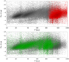 |
Fig. 3 Location of the stars that have LSP as the strongest period in the period vs. Gaia Wesenheit index plane. In the top panel, the stars from the sample are plotted using the LSPs as the period (red). In the bottom panel, the same stars are plotted with the strongest pulsational period (green). Non-LSP LPVs are shown as a background in gray in both panels. |
3.3 Spectroscopic properties
For the purpose of further analysis, we crossmatched our sample with the following catalogs of spectroscopic surveys: APOGEE DR17 (Abdurro’uf et al. 2022), GALAH DR3 (Buder et al. 2021), and RAVE DR6 (Steinmetz et al. 2020). The crossmatch results in 652, 916, and 1877 matches for APOGEE, GALAH, and RAVE, respectively. A first analysis of basic spectroscopic parameters, namely log ɡ and Teff, did not highlight any clear difference between our samples. We also looked into [Fe/H], [M/H], and [α/H] (if available in a given survey). However, the number of objects for which these measurements were available was too small to make a meaningful comparison. We also checked the [Fe/H] value provided in Gaia DR3 (Fig. 12). The LSP stars have a higher metallicity than their non-LSP counterparts.
Next, we checked the C/O ratio in the APOGEE data, which is the only of the three aforementioned surveys that has enough C and O abundance data available to make a statistically significant comparison. The comparison of the C/O distribution for LSP and non-LSP stars is shown in Fig. 13. The LSP stars appear to be more C-rich than the non-LSP ones.
We also used the information about the C/O ratio provided in the Gaia DR3 catalog of Long Period Variables (Lebzelter et al. 2023), based on Gaia spectro-photometric data. The fraction of C-rich stars in the LSP and non-LSP sample is comparable and in general low. In contrast with the APOGEE data, the Gaia chemical classification indicates a slightly lower fraction of C-rich stars − 4% – compared to 5% in the non-LSP LPVs.
To further investigate the C/O ratio of the stars in the sample we used the Gaia-2MASS Wesenheit index, WRP − WJK, adopted from (Lebzelter et al. 2019). This quantity is an indicator of the C/O, as it tends to be larger than 0.8 mag for C-rich stars and smaller than 0.8 mag for O-rich ones. The distribution in the WRP − WJK index is shown in Fig. 14. While the difference between the two distributions seems to be small, it turns out to be statistically significant when tested with the Kolmogorov–Smirnov (KS) test.
Another potentially interesting feature can be observed in the stellar age distribution derived from the RAVE data (Fig. 15). The LSP stars appear to be on average older than the non-LSP stars. The difference in age is small but still statistically significant at a 4% level when tested with the KS test.
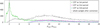 |
Fig. 5 Period ratio for the stars where the LSP was detected as the first period (green), second period (magenta), and third period (blue). The high pick at PLSP/PPULS = 2 is a clear indication that some of the periods identified as pulsational are actually harmonics of the LSP. The whole sample after alias correction is shown in gray. |
3.4 Quality check
As a first quality check, we repeated the analysis, replacing the original comparison sample with the randomized one, and compared the results. The distribution in the randomized control sample is consistent with the base control sample, leading to the conclusion that the construction of the control sample does not introduce a significant bias.
Another potential source of bias is the footprint of the ASAS-SN survey, which is clearly visible in Fig. 7. It results from the fact that the ASAS-SN catalog of variable stars is not homogeneous, as it includes both variable stars discovered independently by ASAS-SN as well as stars from the literature catalogs.
The most prominent feature of this footprint is the artificial over-density stripe around the Galactic equator. In order to make sure that this artifact was not affecting our conclusions, we redid the analysis, excluding the stripe between −5° < b < 5°, where the artifact appears. We obtained results consistent with the original analysis.
We note that, in crowded regions, the flux from unresolved stars can cause the photometric amplitude of a variable star to be underestimated (Riess et al. 2020). Lebzelter et al. (2023) have shown this to be the case for the V-band amplitude of ASAS-SN sources toward the Galactic plane and bulge. As we identify LSPs by their amplitude, this effect could lead us to mistake the pulsation period of a Mira in a crowded sky for an LSP. In order to assess the impact of this effect, we compared the ASAS-SN V-band amplitude with the G-band amplitude from the 2nd Gaia Catalog of Long Period Variable Candidates (Lebzelter et al. 2023). The latter value is expected to be more accurate owing to the higher spatial resolution achieved by Gaia, and is available for about 20 000 objects from our sample. We find that, in most cases, the two amplitudes as well as the two magnitudes appear to be related by a power law, with some scatter (Fig. 16). About 4% of the sources deviate from this pattern and have a rather small V-band amplitude, indicative of the crowding effect.
We repeated our analysis after excluding these sources and found the results to be consistent with the original analysis.
The last check that we made related to the time coverage of the ASAS-SN photometry. While most of the light curves cover more than 1000 days of observation, there is a subset with shorter time coverage. For these objects, the LSPs may not always be reliably detected. As a final quality check, we excluded those stars with less than 1000 days of data and once more redid the analysis. Once again, the results were consistent. We conclude that the aforementioned factors do not introduce a significant bias to our analysis.
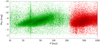 |
Fig. 6 PL after correction. The color schema is the same as in Fig. 3. For the stars that had an LSP detected as the first period and an LSP alias as the second period, the third strongest period was adopted as the pulsational period. |
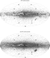 |
Fig. 7 Sky distribution of the two selected samples. The LSP sample is shown in the top panel and the non-LSP sample in the bottom panel. |
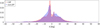 |
Fig. 8 Galactic latitude distribution for LSP and non-LSP stars. The level of statistical significance tested with the KS test is p ≈ 10−16. |
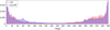 |
Fig. 9 Galactic longitude distribution. The level of statistical significance tested with the KS test is p ≈ 10−16. |
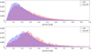 |
Fig. 10 Parallaxes observed toward the Galactic center (upper panel) and the Galactic anti-center (lower panel). |
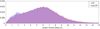 |
Fig. 11 Proper motion distribution. The level of statistical significance tested with the KS test is p = 6.1 × 10⁻¹⁴. |
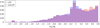 |
Fig. 12 Metallicilty distribution based on the Gaia DR3 data. The level of statistical significance tested with the KS test is p ≈ 10−16. |
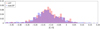 |
Fig. 13 Distribution of the C/O ratio based on the APOGEE data. The level of statistical significance tested with the KS test is p = 0.00083. |
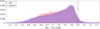 |
Fig. 14 WRP − WJK Gaia-2MASS Wesenheit index, which can be used as an indicator of the C/O status. The level of statistical significance tested with the KS test is p = 1.55 × 10⁻⁸. The vertical dashed line at WRP − WJK = 0.8 marks the boundary between O- and C-rich stars. |
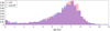 |
Fig. 15 Age distribution based on the RAVE data. The level of statistical significance tested with the KS test is p = 0.043. |
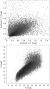 |
Fig. 16 ASAS-SN V-band amplitude vs. Gaia G-band amplitude (top panel) and mean V-band magnitude vs. mean G-band magnitude (bottom panel). |
4 Discussion and conclusions
Our first observation is that most of the LSP stars lie on the first-overtone sequences B and C′. While there are a number of LSP stars that have one of the periods detected in the region roughly consistent with the fundamental mode sequence C, we conclude that these are most likely harmonics of the LSP, not real fundamental mode pulsations.
The fact that the LSP stars appear predominantly on the first-overtone sequences B and C′ is consistent with the previous results of Trabucchi et al. (2017), connecting the LSP to these two sequences and the transition between them. This result suggests that there may indeed be a physical reason tying the LSP phenomenon to the first overtone sequences, but the exact nature of this mechanism remains unclear.
However, it should also be noted that the whole ASAS-SN sample of the LPVs that we used for this search is dominated by first-overtone pulsators. The fact that there are much fewer fundamental mode than overtone pulsators in the base sample may affect the distribution of the selected LSPs. Therefore, this result should be interpreted with caution.
The comparison between the LSP and non-LSP LPVs reveals some subtle but statistically significant differences between the two populations. First, there is a difference between the spatial distribution of the two samples. The LSP stars appear to be more dispersed and less concentrated around the Galactic plane than their non-LSP counterparts, which hints at a possible age difference.
The spectroscopically derived ages from the RAVE catalog seem to support the age difference hypothesis, as the LSP stars appear to be statistically older. It should be noted that the RAVE age estimates carry a high level of uncertainty and the statistical difference between the two distributions is marginally significant. These results therefore need to be interpreted with caution. Being aware of these limitations, the spectroscopic ages may be another hint of a population difference between LSP and non-LSP giants.
Another potentially important feature distinguishing the LSPs from non-LSPs is the C/O ratio, which has a statistically different distribution for the two samples. This can be seen both in the photometric data (WRP − WJK, Gaia-2MASS Wesenheit index) and the specto-photometric classification provided in Gaia DR3, as well as direct spectroscopic measurements. Interestingly, the APOGEE data show a higher C/O ratio for the LSP stars, while the Gaia data seem to show a trend that is harder to interpret. While a statistically significant difference between the two populations can be observed, the direction of the trend is ambiguous. It should be noted that the APOGEE data are only available for a relatively small number of stars, located in very specific sky regions, mostly toward the Galactic bulge, which may affect the result. On the contrary, the Gaia data are all-sky, and therefore more representative of the general picture.
The difference in the C/O ratio is interesting for two reasons. First, the C/O depends on the metallicity (Bensby & Feltzing 2006; Marigo et al. 2020). Therefore, it can be used as an indirect population indicator. The most obvious choice for such an indicator would be [Fe/H] itself. However, the number of objects that have reliable [Fe/H] values in any of the three spectroscopic catalogs used for this study is too small to draw a significant conclusion. Still, the difference in C/O can be interpreted as a hint toward the aforementioned hypothesis about the population difference. A the same time, the [Fe/H] values provided in Gaia DR3 indeed show different distributions, with the LSP having a higher metallicity on average.
Second, the difference in the C/O ratio may also be connected to the high mass-loss rate, as dust-driven wind requires a certain level of carbon abundance to be activated (Lagadec & Zijlstra 2008; Goldman et al. 2017; Marigo et al. 2020). The mass loss and dust production are, in turn, known to be connected to the LSP phenomenon (McDonald & Trabucchi 2019). The dust production becomes especially important in the binarity scenario, which assumes the presence of a dust cloud around a low-mass companion (Soszyński et al. 2021). Therefore, the difference in terms of the C/O ratio between the LSP and non-LSP giants may be seen as an indicator of the binarity hypothesis.
However, the potential population differences are rather subtle, making it hard to draw definitive conclusions. Further studies are required to verify this hypothesis. With coming improved spectroscopic data, the type diagnostics we do will become more stringent, or will be able to confirm the tendencies we see.
Acknowledgements
M.P. is supported by the SONATINA grant 2020/36/C/ST9/00103 from the Polish National Science Center and the BEKKER fellowship BPN/BEK/2022/1/00106 from the Polish National Agency for Academic Exchange. L.E. and M.P. acknowledge the funding of the Department of Astronomy of the University of Geneva. M.T. and N.M. acknowledge the support provided by the Swiss National Science Foundation through grant Nr. 188697. M.T. acknowledges support from Padova University through the research project PRD 2021. This work made extensive use of TOPCAT (Taylor 2005) and VARTOOLS (Hartman & Bakos 2016). This work has made use of data from the European Space Agency (ESA) mission Gaia (https://www.cosmos.esa.int/gaia), processed by the Gaia Data Processing and Analysis Consortium (DPAC, https://www.cosmos.esa.int/web/gaia/dpac/consortium). Funding for the DPAC has been provided by national institutions, in particular the institutions participating in the Gaia Multilateral Agreement.
References
- Abdurro’uf, A. K., Aerts, C., Silva Aguirre, V., et al. 2022, ApJS, 259, 354 [Google Scholar]
- Bensby, T., & Feltzing, S. 2006, MNRAS, 367, 1181 [CrossRef] [Google Scholar]
- Buder, S., Sharma, S., Kos, J., et al. 2021, MNRAS, 506, 150 [NASA ADS] [CrossRef] [Google Scholar]
- De Silva, G. M., Freeman, K. C., Bland-Hawthorn, J., et al. 2015, MNRAS, 449, 2604 [NASA ADS] [CrossRef] [Google Scholar]
- Gaia Collaboration (Brown, A. G. A., et al.) 2021, A&A, 649, A1 [NASA ADS] [CrossRef] [EDP Sciences] [Google Scholar]
- Gaia Collaboration (Vallenari, A., et al.) 2023, A&A, 674, A1 [NASA ADS] [CrossRef] [EDP Sciences] [Google Scholar]
- Goldman S. R., van Loon J. T., Zijlstra A. A., et al. 2017, MNRAS, 465, 403 [CrossRef] [Google Scholar]
- Hartman, J. D., & Bakos, G. Á. 2016, Astron. Comput., 17, 1 [Google Scholar]
- Hinkle, K. H., Lebzelter, T., Joyce, R. R., & Fekel, F. C. 2002, AJ, 123, 1002 [Google Scholar]
- Houk, N. 1963, AJ, 68, 253 [Google Scholar]
- Jayasinghe, T., Kochanek, C. S., Stanek, K. Z., et al. 2018, MNRAS, 477, 3145 [Google Scholar]
- Jayasinghe, T., Stanek, K. Z., Kochanek, C. S., et al. 2019a, MNRAS, 486, 1907 [NASA ADS] [Google Scholar]
- Jayasinghe, T., Stanek, K. Z., Kochanek, C. S., et al. 2019b, MNRAS, 485, 961 [Google Scholar]
- Jayasinghe, T., Kochanek, C. S., Stanek, K. Z., et al. 2021, MNRAS, 503, 200 [NASA ADS] [CrossRef] [Google Scholar]
- Lagadec, E., & Zijlstra, A. A. 2008, MNRAS, 390, L59 [NASA ADS] [CrossRef] [Google Scholar]
- Lebzelter, T., Trabucchi, M., Mowlavi, N., et al. 2019, A&A, 631, A24 [NASA ADS] [CrossRef] [EDP Sciences] [Google Scholar]
- Lebzelter, T., Mowlavi, N., Lecoeur-Taibi, I., et al. 2023, A&A, 674, A15 [NASA ADS] [CrossRef] [EDP Sciences] [Google Scholar]
- McDonald, I., & Trabucchi, M. 2019, MNRAS, 484, 4678 [Google Scholar]
- Majewski, S. R., Schiavon, R. P., Frinchaboy, P. M., et al. 2017, AJ, 154, 94 [NASA ADS] [CrossRef] [Google Scholar]
- Marigo, P., Cummings, J. D., Curtis, J. L., et al. 2020, Nat. Astron., 4, 1102 [NASA ADS] [CrossRef] [Google Scholar]
- Nicholls, C. P., Wood, P. R., Cioni, M.-R. L., & Soszynski, I. 2009, MNRAS, 399, 2063 [CrossRef] [Google Scholar]
- O’Connell, D. J. K. 1933, Harvard Coll. Observ. Bull., 893, 19 [Google Scholar]
- Pawlak, M. 2021, A&A, 649, A110 [NASA ADS] [CrossRef] [EDP Sciences] [Google Scholar]
- Pawlak, M., Pejcha, O., Jakucík, P., et al. 2019, MNRAS, 487, 5932 [NASA ADS] [CrossRef] [Google Scholar]
- Payne-Gaposchkin, C. 1954, Ann. Harvard Coll. Observ., 113, 189 [NASA ADS] [Google Scholar]
- Riess, A. G., Yuan, W., Casertano, S., Macri, L. M., & Scolnic, D. 2020, ApJ, 896, L43 [Google Scholar]
- Saio, H., Wood, P. R., Takayama, M., & Ita, Y. 2015, MNRAS, 452, 3863 [Google Scholar]
- Shappee, B. J., Prieto, J. L., Grupe, D., et al. 2014, ApJ, 788, 48 [Google Scholar]
- Soszyński, I. 2007, ApJ, 660, 1486 [Google Scholar]
- Soszyński, I., & Udalski, A. 2014, ApJ, 788, 13 [Google Scholar]
- Soszyński, I., Udalski, A., Szymanski, M. K., et al. 2009, Acta Astron., 59, 239 [Google Scholar]
- Soszyński, I., Olechowska, A., Ratajczak, M., et al. 2021, ApJ, 911, L22 [CrossRef] [Google Scholar]
- Steinmetz, M., Zwitter, T., Siebert, A., et al. 2006, AJ, 132, 1645 [Google Scholar]
- Steinmetz, M., Guiglion, G., McMillan, P. J., et al. 2020, AJ, 160, 83 [NASA ADS] [CrossRef] [Google Scholar]
- Taylor, M. B. 2005, ASP Conf. Ser., 347, 29 [Google Scholar]
- Trabucchi, M., Wood, P. R., Montalbán, J., et al. 2017, ApJ, 847, 139 [Google Scholar]
- Wood, P. R. 2000a, IAU Colloq. 176: The Impact of Large-Scale Surveys on Pulsating Star Research, 203, 379 [Google Scholar]
- Wood, P. R. 2000b, PASA, 17, 18 [Google Scholar]
- Wood P. R. 2015, MNRAS, 448, 3829 [CrossRef] [Google Scholar]
- Wood, P. R., Alcock, C., Allsman, R. A., et al. 1999, Asymptotic Giant Branch Stars, 191, 151 [Google Scholar]
- Wood, P. R., Olivier, E. A., & Kawaler, S. D. 2004, ApJ, 604, 800 [Google Scholar]
All Figures
|
Fig. 1 Selection of the LSP stars based on the location on the period-amplitude diagram. Periods selected as LSPs are marked in magenta, while other LPVs are marked in gray. The cutoff criterion is A < 1.6 log(P) − 3.7, and is marked with a dashed black line. |
| In the text | |
|
Fig. 2 Verification of the selection criterion using the OGLE LMC sample (Soszyński et al. 2007). The period-amplitude cutoff marked with dashed line is the same as in Fig. 1. The objects selected with the cutoff (upper panel) are placed on the PL diagram (lower panel). For the PL diagram, we use the redenig-free Wesenheit index WI = V − 1.55(V − I). |
| In the text | |
|
Fig. 3 Location of the stars that have LSP as the strongest period in the period vs. Gaia Wesenheit index plane. In the top panel, the stars from the sample are plotted using the LSPs as the period (red). In the bottom panel, the same stars are plotted with the strongest pulsational period (green). Non-LSP LPVs are shown as a background in gray in both panels. |
| In the text | |
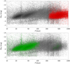 |
Fig. 4 Same as Fig. 3, but for the stars that have an LSP as a second or third period. |
| In the text | |
|
Fig. 5 Period ratio for the stars where the LSP was detected as the first period (green), second period (magenta), and third period (blue). The high pick at PLSP/PPULS = 2 is a clear indication that some of the periods identified as pulsational are actually harmonics of the LSP. The whole sample after alias correction is shown in gray. |
| In the text | |
|
Fig. 6 PL after correction. The color schema is the same as in Fig. 3. For the stars that had an LSP detected as the first period and an LSP alias as the second period, the third strongest period was adopted as the pulsational period. |
| In the text | |
|
Fig. 7 Sky distribution of the two selected samples. The LSP sample is shown in the top panel and the non-LSP sample in the bottom panel. |
| In the text | |
|
Fig. 8 Galactic latitude distribution for LSP and non-LSP stars. The level of statistical significance tested with the KS test is p ≈ 10−16. |
| In the text | |
|
Fig. 9 Galactic longitude distribution. The level of statistical significance tested with the KS test is p ≈ 10−16. |
| In the text | |
|
Fig. 10 Parallaxes observed toward the Galactic center (upper panel) and the Galactic anti-center (lower panel). |
| In the text | |
|
Fig. 11 Proper motion distribution. The level of statistical significance tested with the KS test is p = 6.1 × 10⁻¹⁴. |
| In the text | |
|
Fig. 12 Metallicilty distribution based on the Gaia DR3 data. The level of statistical significance tested with the KS test is p ≈ 10−16. |
| In the text | |
|
Fig. 13 Distribution of the C/O ratio based on the APOGEE data. The level of statistical significance tested with the KS test is p = 0.00083. |
| In the text | |
|
Fig. 14 WRP − WJK Gaia-2MASS Wesenheit index, which can be used as an indicator of the C/O status. The level of statistical significance tested with the KS test is p = 1.55 × 10⁻⁸. The vertical dashed line at WRP − WJK = 0.8 marks the boundary between O- and C-rich stars. |
| In the text | |
|
Fig. 15 Age distribution based on the RAVE data. The level of statistical significance tested with the KS test is p = 0.043. |
| In the text | |
|
Fig. 16 ASAS-SN V-band amplitude vs. Gaia G-band amplitude (top panel) and mean V-band magnitude vs. mean G-band magnitude (bottom panel). |
| In the text | |
Current usage metrics show cumulative count of Article Views (full-text article views including HTML views, PDF and ePub downloads, according to the available data) and Abstracts Views on Vision4Press platform.
Data correspond to usage on the plateform after 2015. The current usage metrics is available 48-96 hours after online publication and is updated daily on week days.
Initial download of the metrics may take a while.