| Issue |
A&A
Volume 709, May 2026
|
|
|---|---|---|
| Article Number | A150 | |
| Number of page(s) | 10 | |
| Section | Extragalactic astronomy | |
| DOI | https://doi.org/10.1051/0004-6361/202558716 | |
| Published online | 13 May 2026 | |
The IXPE and multifrequency polarimetric view of the extreme blazars 1ES 1101-232 and RGB J0710+591
1
INAF – Osservatorio Astronomico di Brera, Via E. Bianchi 46, I-23807 Merate, Italy
2
INAF – Istituto di Astrofisica e Planetologia Spaziali, Via Fosso del Cavaliere, 100, I-00133 Rome, Italy
3
Instituto de Astrofísica de Andalucía, IAA-CSIC, Glorieta de la Astronomía s/n, 18008 Granada, Spain
4
Institute of Astrophysics, Foundation for Research and Technology-Hellas, Vasilika Vouton, GR-70013 Heraklion, Greece
5
Department of Astronomy, Yale University, PO Box 208101 New Haven, CT 06520-8101, USA
6
ASI – Agenzia Spaziale Italiana, Via del Politecnico snc, 00133 Roma, Italy
7
European Space Astronomy Centre (ESA/ESAC), 28691 Villanueva de la Canada, Madrid, Spain
8
NASA Marshall Space Flight Center, Huntsville, AL 35812, USA
9
Department of Physics, University of Crete, Voutes University Campus, 70013 Heraklion, Greece
10
Center for Astrophysics | Harvard & Smithsonian, 60 Garden Street, Cambridge, MA 02138, USA
11
Istituto Nazionale di Fisica Nucleare, Sezione di Padova, 35131 Padova, Italy
12
Department of Physics and Astronomy, 20014 University of Turku, Turku, Finland
13
Finnish Centre for Astronomy with ESO, 20014 University of Turku, Turku, Finland
14
Instituto de Radioastronomía Millimétrica, Avenida Divina Pastora, 7, Local 20, E-18012 Granada, Spain
15
Orchideenweg 8, 53123 Bonn, Germany
16
Max-Planck-Institut für Radioastronomie, Auf dem Hügel 69, D-53121 Bonn, Germany
17
Department of Physics, Graduate School of Advanced Science and Engineering, Hiroshima University Kagamiyama, 1-3-1 Higashi-Hiroshima, Hiroshima 739-8526, Japan
18
Department of Physics, Tokyo Institute of Technology, 2-12-1 Ookayama, Meguro-ku, Tokyo 152-8551, Japan
19
Hiroshima Astrophysical Science Center, Hiroshima University, 1-3-1 Kagamiyama, Higashi-Hiroshima, Hiroshima 739-8526, Japan
20
Core Research for Energetic Universe (Core-U), Hiroshima University, 1-3-1 Kagamiyama, Higashi-Hiroshima, Hiroshima 739-8526, Japan
21
Planetary Exploration Research Center, Chiba Institute of Technology, 2-17-1 Tsudanuma, Narashino, Chiba 275-0016, Japan
22
Institute of Astronomy and NAO, Bulgarian Academy of Sciences, 1784 Sofia, Bulgaria
23
GFZ Helmholtz Centre for Geosciences, Telegrafenberg, 14476 Potsdam, Germany
24
Julius-Maximilians-Universität Würzburg, Institut für Theoretische Physik und Astrophysik, Lehrstuhl für Astronomie, Emil-Fischer-Straße 31, 97074 Würzburg, Germany
25
Physics Department and McDonnell Center for the Space Sciences, Washington University in St. Louis, St. Louis, MO 63130, USA
26
Dr. Karl-Remeis Sternwarte and Erlangen Centre for Astroparticle Physics, Friedrich-Alexander Universität Erlangen-Nürnberg, Sternwartstr. 7, 96049 Bamberg, Germany
27
Korea Astronomy and Space Science Institute, 776 Daedeok-daero, Yuseong-gu, Daejeon 34055, Korea
28
University of Science and Technology, Korea, 217 Gajeong-ro, Yuseong-gu, Daejeon 34113, Korea
★ Corresponding author: This email address is being protected from spambots. You need JavaScript enabled to view it.
Received:
22
December
2025
Accepted:
15
March
2026
Abstract
Multiwavelength polarimetry offers a powerful tool to probe magnetic field and flow geometries in the relativistic jets of blazars. Sources with synchrotron emission that spans a broad frequency range, from radio to X-rays, such as High Synchrotron Peak (HSP) type BL Lac objects, are particularly interesting. Previous measurements including radio, optical, and X-ray data show a clear trend, with the degree of polarization increasing with frequency. Here we report radio, optical, and X-ray observations (Swift, Nustar, and IXPE) of 1ES 1101-232 and RGB J0710+591, two blazars belonging to the puzzling subclass of extreme BL Lacs (EHBL). For 1ES 1101-232, we find a strong frequency dependence of the degree of polarization, with a ratio ΠX/ΠO ≃ 5.2. For RGB J0710+591, IXPE derives a 1σ upper limit ΠX < 11.6%, comparable to the measured optical degree of polarization (average ΠO ∼ 12%). We discuss the results in the framework of current interpretations and, in particular, we report an improved version of the stratified shock model that reproduces the observed data of both sources.
Key words: acceleration of particles / polarization / radiation mechanisms: non-thermal / BL Lacertae objects: individual: 1ES 1101-232 / BL Lacertae objects: individual: RGB J0710+591 / galaxies: jets
© The Authors 2026
 Open Access article, published by EDP Sciences, under the terms of the Creative Commons Attribution License (https://creativecommons.org/licenses/by/4.0), which permits unrestricted use, distribution, and reproduction in any medium, provided the original work is properly cited.
This article is published in open access under the Subscribe to Open model. This email address is being protected from spambots. You need JavaScript enabled to view it. to support open access publication.
1. Introduction
Despite decades of observational and theoretical efforts, the physical processes acting in relativistic jets remain partially unknown. Basic questions concerning, for example, the matter content of the jet, the role of the magnetic field, and the emission mechanisms remain open (Blandford et al. 2019). One of the most central topics concerns the mechanisms that energize the emitting particles at the required ultra-relativistic energies. In the past, shocks were identified as the most likely acceleration sites (e.g. Blandford & Eichler 1987), but recent studies highlight the potential roles of magnetic reconnection and turbulence (e.g., Matthews et al. 2020).
Blazars provide the best means to study the physical processes in the jet near the central engine, due to the relativistic amplification of their jet emission caused by favorable alignment (Blandford et al. 2019; Romero et al. 2017). The emission from this class of sources spans the entire electromagnetic spectrum, from radio waves up to high-energy γ rays (Fossati et al. 1998). The “double hump” shape of the spectral energy distribution (SED) indicates the presence of two emission components. The low-energy bump (peaking, depending on the source type, from IR to the X-ray band) is produced by electrons located at distances on the order of 100–1000 gravitational radii from the central black hole through synchrotron emission. The origin of the high-energy component remains debated, with leptonic and hadronic models as contenders (e.g. Cerruti 2020; Sol & Zech 2022). Most models used to reproduce the emission of blazars (both leptonic and hadronic) adopt a one-zone scenario, which assumes that most of the radiation originates from particles within a unique region of the jet characterized by a homogeneous physical structure.
High-synchrotron peaked (HSP) blazars, where the synchrotron component peaks in the X-ray band and the high-energy component reaches TeV energies, are particularly interesting for studies of particle acceleration mechanisms. Their intense X-ray emission allows detailed probing of the dynamics of the emitting particles and tracking of the main processes at work (e.g., acceleration, cooling) at the rapidly-evolving, high-energy tail of the electron energy distribution. Due to the short cooling length of electrons emitting at these energies, their emission can be used to probe regions in the vicinity of the acceleration site. In particular, the polarization properties in this band could be exploited to discriminate among the potential acceleration mechanisms at work (Tavecchio 2021). Moreover, the highly successful IXPE observations of a handful of HSPs strongly support shocks as the main actors in the acceleration process (Liodakis et al. 2022) and, for the first time, enable a physical description of the emission regions1. In particular, HSPs commonly show a strong frequency-dependent polarization fraction (see, e.g., Kim et al. 2024b), as expected from the “stratified shock” scenario (Angelakis et al. 2016; Tavecchio et al. 2018). In this model, contrary to the widely adopted one-zone scheme, electrons accelerated at the shock cool within an energy-dependent distance of the downstream flow and experience different degrees of magnetic field order, which are eventually encoded in the polarization (but see Bolis et al. 2024 for an alternative view).
Among HSPs, the group of extreme HSPs (EHBLs) (Costamante et al. 2001) is attracting growing attention because their unusual properties are difficult to reproduce within the framework of standard models (Katarzyński et al. 2006; Bonnoli et al. 2015; Costamante et al. 2018; Biteau et al. 2020). At odds with the bulk of the blazar population, their SED is generally stable, showing only weak (factor of two) variability over long timescales (weeks). Moreover, their extremely hard γ-ray continuum (with the peak of the high-energy component above 10 TeV) is difficult to interpret using standard models based on inverse Compton emission (e.g., Biteau et al. 2020). The unusual phenomenology of EHBLs has been explained by invoking a hard electron distribution with a large minimum energy (Katarzyński et al. 2006; Tavecchio et al. 2009), a Maxwellian-like electron distribution (Lefa et al. 2011), internal absorption (Aharonian et al. 2008) or emission from a large-scale jet (Böttcher et al. 2008). Recent studies interpret the peculiarities of EHBLs as arising from a particular shape of the energy distribution of the emitting electrons, produced either by multiple shocks (Zech & Lemoine 2021) or by acceleration through turbulence (Tavecchio et al. 2022; Sciaccaluga & Tavecchio 2022). In any case, the phenomenology of EHBLs provides access to one of the most extreme facets of acceleration in jets. The IXPE mission observed the prototypical source of this class, 1ES0229+200, revealing the most energy-dependent degree of polarization among HSPs, with 18% in X-rays and 3% in the optical band (as measured with the Nordic Optical Telescope and Observatorio de Sierra Nevada telescopes; Ehlert et al. 2023). The pronounced chromaticity of the polarization may be related to the extreme nature of these sources.
To enlarge the sample of EHBLs with polarimetric information and investigate the possible connections with their peculiar phenomenology, we requested IXPE pointings of two X-ray bright EHBLs, namely 1ES 1101-232 and RGB J0710+591 (Costamante et al. 2018). We complemented the IXPE observations with contemporaneous millimeter, optical, and X-ray observations using Swift and NuStarto ensure good coverage of the synchrotron peak and its polarimetric properties. In this paper, we report the multiwavelength data, including polarimetric measurements, for the two sources, and we discuss the results in the framework of the stratified shock scenario.
The paper is organized as follows. In Sect. 2, we present the observations and the data analysis; in Sect. 3, we present the results; and in Sect. 4, we discuss our findings.
Throughout the paper, we assume the following cosmological parameters: H0 = 67 km s−1 Mpc−1, ΩM = 0.3, and ΩΛ = 0.7 (e.g., Planck Collaboration VI 2020).
2. Observations and data analysis
2.1. IXPE
Observations of two EHBLs with IXPE were conducted for 1ES 1101-232 (Obs. ID 03006901; 28 November 2024 to 02 December 2024; for ∼190 ks) and RGB J0710+591 (Obs. ID 03007099; 20 March 2024 to 14 April 2024; for ∼285 ks). We estimated X-ray polarization for each observation using both event-by-event Stokes parameter analysis (Kislat et al. 2015, the so-called model-independent analysis) and spectropolarimetric analysis (Strohmayer 2017). In the event-by-event Stokes parameter analysis, we derived the polarization degree (ΠX) and polarization angle (ψX) from the normalized Stokes parameters q and u, obtained from the pcube products generated by the xpbin task in the ixpeobssim software (Baldini et al. 2022), using the relations  and
and  . We performed spectropolarimetric analysis with the conventional X-ray spectral fitting tool XSPEC (version 12; Arnaud 1996) on the I, Q, and U spectra. We modeled the spectra using the logpar model Massaro et al. (2004) to reproduce the synchrotron emission from the jets, together with a constant polarization model (polconst) to estimate the polarization properties. The pivotE parameter was fixed at 2 keV. Additionally, we accounted for cross-calibration factors between the three detector units (DUs) using constant, and modeled Galactic absorption with tbabs, adopting the weighted average column density values from HI4PI Collaboration (2016), with
  for 1ES 1101-232 and
  for RGB J0710+591. We used the willm model to account for metal abundances (Wilms et al. 2000). We estimated errors in both analysis methods following the guidelines provided by the IXPE Science Team2. We also applied the background rejection algorithm (Di Marco et al. 2022) to improve the sensitivity of the measurements. The overall data processing followed the procedures described in Kim et al. (2024a), as applied in previous IXPE observations of blazars. For calibration, we employed the most recent versions of the IXPE XRT calibration database (version 20241028) and the IXPE GPD calibration database (version 20250225). We carried out all processing using ixpeobssim version 31.0.3 and HEASOFT version 6.34. For each source, we independently cross-validated the event-by-event Stokes parameter analysis and the spectropolarimetric analysis, yielding results that are statistically consistent within the uncertainties. (e.g., Kim et al. 2024a)
We measured the time-averaged polarization over the full duration of each observation in the 2–8 keV energy band. For 1ES 1101-232, the PCUBE analysis yielded a polarization degree of ΠX = 15.9%±3.8% and a polarization angle of ψX = 15.7° ±6.8°. The spectropolarimetric analysis constrained the polarization to ΠX = 16.3%±2.7% and ψX = 12.2° ±4.7°. For RGB J0710+591, we did not significantly detect X-ray polarization. The PCUBE analysis provided a 99% confidence level upper limit of ΠX < 13.0%, while the spectropolarimetric analysis yielded a slightly tighter, but consistent, 99% confidence-level upper limit of ΠX < 11.6%. Figure 1 illustrates the measured X-ray polarization from the spectropolarimetric analysis, showing the detection significance across the polarization degree and angle parameter space for each observation. Table 1 summarizes the spectral fitting results for each observation.
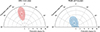 |
Fig. 1. Detection significance of X-ray polarization for 1ES 1101-232 (left) and RGB J0710+591 (right), as measured from the spectropolarimetric analysis. The tangential direction indicates the polarization angle, and the radial direction corresponds to the polarization degree. The colored dot at the center of each contour denotes the measured X-ray polarization. Contours correspond to detection confidence levels of 68%, 90%, and 99%. |
Best-fit parameters from the spectropolarimetric analyses of 1ES 1101-232 and RGB J0710+591.
To investigate the potential variability of the polarization over time, we conducted a time-resolved analysis. We estimated the null hypothesis probability for fitting a constant model to the q and u Stokes parameters independently, dividing the entire observation according to integer ratios from two to 15, following the method presented in Kim et al. (2024a). For both observations, the null hypothesis probabilities for the constant model fits to the q and u Stokes parameters exceeded 1%, indicating no significant deviation from a constant polarization signal. Thus, the observed polarization variations are consistent with random fluctuations. In particular, as an additional test for RGB J0710+591, we considered the observational gap in the middle of the exposure (Figure 2) and divided the dataset into period one (P1; green shaded area) and two (P2; orange shaded area) and measured the time-averaged polarization separately. However, despite a slight increase in significance in P2, the polarization remained unconstrained.
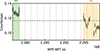 |
Fig. 2. Light curve of the IXPE observation of RGB J0710+591. The green and orange shaded areas indicate periods one and two, respectively, split according to the central observation gap. The central dashed green line represents the average count rate of RGB J0710+591 during the IXPE observation. |
We also performed an energy-resolved analysis by subdividing the IXPE energy range (2–8 keV) into narrower intervals, beginning with two bins (2–4 keV and 4–8 keV), then three bins (2–4, 4–6, and 6–8 keV), and extending up to 12 bins in total. The results show no statistically significant variation relative to a constant model, indicating that the X-ray polarization remains consistent across energy and exhibits no energy dependence. Notably, in the 3–4 keV range, the PCUBE analysis of RGB J0710+591 detects a polarization signal corresponding to ΠX = 16.6%±5.2% and ψX = 32.6° ±9.0° at the 99.4% confidence level. However, this signal was not reproduced in the spectropolarimetric analysis with XSPEC, likely because XSPEC estimates uncertainties based on chi-square statistics, which provides low significance when using such a narrow energy bin (3–4 keV) with large uncertainty.
We performed a joint spectropolarimetric analysis including Swift and NuSTAR (details below). We applied the same spectral model used in the IXPE-only analysis: constant×tbabs×polconst×logpar. We fixed constant as unity for Swift spectra as a reference and allowed it to vary for the others. Table 2 presents the results of the joint spectral model, and Figs. 3 and 4 show the spectral fits. This yields slightly improved constraints on both spectral and polarization properties. Although the logpar alpha parameter, which indicates the spectral slope, deviates for 1ES 1101-232, other parameters, including polarization properties, remain consistent within uncertainties. The joint analysis yields ΠX = 15.7%±2.6% and ψX = 12.2° ±4.7° for 1ES 1101-232, and a 99% confidence level upper limit of ΠX < 12.2% for RGB J0710+591.
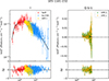 |
Fig. 3. Joint spectropolarimetric analysis of 1ES 1101-232. Left: Energy flux spectra, expressed as photon flux multiplied by energy squared, for the Swift (red), IXPE I (yellow), and NuSTAR (blue) data together with the corresponding data-model residuals. The black line indicates the best-fit model. Right: IXPE Q and U spectra, displayed in green and orange, respectively, together with their deviations from the best-fit model. |
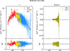 |
Fig. 4. Joint spectropolarimetric analysis of RGB J0710+591. The panels follow the same format as in Figure 3. |
Best-fit parameters from the joint spectropolarimetric analyses of 1ES 1101-232 and RGB J0710+591.
2.2. Swift/XRT
The Swift satellite observed the two sources simultaneously to the IXPE observations: 1ES1101-232 on 28 and 29 November 2024 (ObsIDs: 00035013052-00035013053) and 1, 2, and 4 December 2024 (ObsIDa: 00035013055-00035013057), and RGBJ0710+591 on 4, 9, 11, 13 and 15 April 2024 (ObsID: 00031356080-00031356082, 00031356084, and 00031356085). We downloaded data from the X-ray Telescope (XRT; Burrows et al. 2005) via the HEASARC public archive and processed them using the Swift XRT Data Analysis Software (SWXRTDAS; version 3.7.0) and the relevant software included in HEASOFT v. 6.36. The calibration database was updated on 9 June 2025.
The total exposure of 1ES1101-232 on the XRT was 4.7 ks. We fit the data using a simple power-law model with Galactic absorption (NH = 7.03 × 1020 cm−2; Willingale et al. 2013), using unbinned likelihood (Cash 1979). The model yields Γ = 2.01 ± 0.05 and an integrated observed flux  . We also fit the individual observations separately, yielding significantly consistent flux and photon index values.
RGBJ0710+591 was observed by XRT for a total of 9.8 ks. We fit the data under the same assumptions as for 1ES1101-232, with Galactic absorption NH = 5.15 × 1020 cm−2 and a single power law. Fitting the individual observations separately reveals no variability; therefore, we combine all of them in a single fit. The data are best fit with Γ = 1.86 ± 0.04 and  .
.
2.3. NuSTAR
Simultaneous NuSTAR observations were obtained during IXPE observations for both targets (1ES1101-232: Obs. ID 61001017002; RGBJ0710+591: Obs. IDs 91001607002 and 91001607004) to better constrain the spectral properties by extending the energy range in combination with IXPE. We performed NuSTAR data reduction using nustardas version 2.1.5 and CALDB version 20241216, following the procedures described in the NuSTAR data analysis software user guide3. We generated the level 2 event files for both the FPMA and FPMB detectors using the nupipeline task, and we produced high-level scientific data products, including spectral extractions, using the nuproducts tool. We applied a circular source region with a 1′ radius and a circular background region with a 2′ radius for the source and background extraction. We grouped each spectrum to ensure a minimum of 30 counts per bin. To enable simultaneous spectropolarimetric analysis with IXPE, “XFLT0001 Stokes:0” keyword was added to the header, allowing XSPEC to identify the spectra as Stokes I spectra.
2.4. Optical, millimeter-wave, and radio observations
Optical and radio-millimeter polarization observations were obtained for both sources using the Calar Alto Faint Object Spectrograph (CAFOS; Escudero Pedrosa et al. 2024a) on the Calar Alto 2.2 m Telescope, the DIPOL-1 polarimeter at the Sierra Nevada Observatory (DIPOL-1; Otero-Santos et al. 2024) using the IOP4 data reduction pipeline, (Escudero Pedrosa et al. 2024b,a), the Alhambra Faint Object Spectrograph and Camera (ALFOSC) at the Nordic Optical Telescope (NOT; Nilsson et al. 2018), the KANATA telescope using the Hiroshima Optical and Near-InfraRed camera (HONIR; Kawabata et al. 1999; Akitaya et al. 2014), the 60 cm telescope at the Belogradchik Observatory (Bachev 2024), the SMA Monitoring of AGN with POLarization (SMAPOL) program (Myserlis et al. 2025), and the Effelsberg 100-m telescope through the monitoring the Stokes Q, U, I, and V emission of AGN jets in Radio (QUIVER; Kraus et al. 2003; Myserlis et al. 2018, 2025) and the Tev Effelsberg Long-term Agn MONitoring (TELAMON, Eppel et al. 2024) programs. We reduced all optical observations following standard calibration procedures using polarized and unpolarized standard stars to account for instrumental polarization. Where possible, we corrected the R-band measurements for the depolarizing effect of the host-galaxy flux using the galaxy profiles from Falomo & Ulrich (2000), Nilsson et al. (2007), following Hovatta et al. (2016). Figures 5 and 6 show the optical polarization observations. Although we did not correct some measurements for 1ES 1101-232, the effect on the net polarization is small.
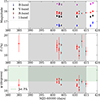 |
Fig. 5. Optical polarization observations of RGB J0710+591. Top: Brightness in different optical bands. Middle: R-band polarization degree. Bottom: Polarization angle. The gray shaded area marks the duration of the IXPE observation, and the horizontal green band marks the jet direction as projected on the sky. |
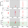 |
Fig. 6. Optical polarization observations of 1ES 1101-232. Panels and symbols are as in Fig. 5. The R-band† measurements (purple symbols) have not been corrected for the host-galaxy contribution. |
RGB J0710+591 shows a very high degree of optical polarization, with a median and standard deviation during the IXPE observation of ΠO = 13.9% and σΠO = 1.8%. In contrast, the radio polarization observations yield only upper limits (at the 3σ level) of < 15% at 2.5 GHz, < 9.8% at 4.8 GHz, < 3% at 6.6 GHz, < 30% at 10.4 GHz, < 3% at 13.6 GHz, and < 6.9% at 225.5 GHz. The median optical polarization angle for the duration of the IXPE is ψO = 18.3 degrees with a standard deviation of σψO = 3. Estimates of the direction of the jet vary between 10–50 degrees Wu et al. (2012), Hovatta et al. (2016), Plavin et al. (2022), with an average of 26 degrees and a wide opening angle of 45 degrees Wu et al. (2012). Although very-long-baseline interferometry (VLBI) observations are not contemporaneous with optical observations, the latter align fairly well with the jet axis, as is often the case for HSP sources (Liodakis et al. 2022; Kouch et al. 2024; Capecchiacci et al. 2025).
Compared to RGB J0710+591, 1ES 1101-232 shows much lower polarization, with a median and standard deviation over the IXPE observation of ΠO = 3.1% and σΠO = 0.4% and a median polarization angle of ψO = 51.7 degrees with a standard deviation of σψO = 3.4. The optical ψO is also fairly aligned with the jet axis in this source (Benke et al. 2024).
3. Results
As expected from the low variability typical of EHBLs, the spectral parameters of the fit X-ray spectrum (including those of the two sources Swift and NuSTAR) are very similar to those reported by Costamante et al. (2018), which also included NuSTAR data. In both cases, the synchrotron component, well reproduced by a log-parabolic shape, peaks around 1 keV. Therefore, IXPE measurements probe the high-energy tail of the synchrotron emission just beyond the peak (see Figs. 3–4).
For RGB J0710+591, we derive a relatively stringent upper limit on the X-ray polarization, even when splitting the data in energy and time. Interestingly, the upper limit is below (or at least comparable at the 3σ confidence level to) the galaxy-corrected optical degree of polarization. These measurements are in contrast to previous results for HBL and EHBL BL Lacs, which are characterized by a pronounced increase of the degree of polarization with frequency, typically ΠX ≳ 2 ΠO (e.g. Kim et al. 2024b; Marscher et al. 2024). The only exception is the HBL 1ES 1959+650, which during a pointing in June 2022 displayed ΠO = 4.7 and ΠX < 5.1 (Errando et al. 2024)4. The prototypical EHBL 1ES 0229+220 represents one of the most extreme cases of chromaticity, with ΠX/ΠO ∼ 6 (Ehlert et al. 2023).
By contrast, 1ES 1101-232 appears consistent with typical BL Lacs, with highly polarized X-ray emission (ΠX ≃ 16%) and relatively modest polarization in the optical band (ΠO ≃ 3%) which translate into a ratio ΠX/ΠO ∼ 5.
In both sources, the optical EVPA is consistent with the jet PA, again in agreement with the typical behavior of HBLs (e.g. Kim et al. 2024b; Marscher et al. 2024). For 1ES 1101-232, ΨX instead lies in the range 8–16 degrees, inconsistent with the optical EVPA (ΨO ∼ 51 degrees) and with the jet PA. Interestingly, while most BL Lac show substantial agreement between ΨX and the jet PA (e.g., Capecchiacci et al. 2025), the prototypical EHBL 1ES 0229+220 also shows an X-ray EVPA misaligned with respect to the jet PA by about 50 degrees. In considering these results, it is important to note that the jet could bend by tens of degrees between the inner region (where the X-ray and optical emission are likely produced) and the outer region imaged in the radio band (e.g. Di Gesu et al. 2022). Moreover, jets can change PA with time (Kostrichkin et al. 2025), while in most cases the radio, optical, and X-ray observations are not simultaneous.
4. Discussion
Our polarimetric measurements of two EHBLs with similar spectral energy distributions (Costamante et al. 2018) add complexity to the observational framework of extreme blazars.
1ES 1101-232, which displays high X-ray polarization but modest optical polarization, follows the trend commonly observed in these types of sources. The ratio of X-ray to optical polarization, ΠX/ΠO ≃ 5.2, is similar to that of the EHBL prototype 1ES 0229+200, with ΠX/ΠO ≃ 5.6 (Ehlert et al. 2023)5. In contrast, the upper limit obtained for RGB J0710+591, together with the large optical polarization (some data points reaching 15% %, the highest value recorded among HBLs and EHBLs monitored by IXPE, Kim et al. 2024b) demonstrates that not all sources follow the simple trend of increasing polarization with frequency.
4.1. A stratified shock model
The observed strong chromaticity in the polarization degree often supports the stratified shock scenario (e.g., Angelakis et al. 2016; Tavecchio et al. 2018; Tavecchio 2021; Marscher & Jorstad 2022). In this model, particles are injected at a shock in the jet and further advected by the downstream flow. Due to the energy-dependent electron cooling time, X-rays are produced very close to the shock, where the field component orthogonal to the shock is more coherent due to compression and kinetic effects. Electrons producing the optical emission have a longer cooling length and fill a large portion of the post-shock fluid, likely experiencing more turbulent and less coherent fields, resulting in a small degree of polarization.
Despite its simplicity, the stratified shock scenario is sufficiently versatile to reproduce the different behavior of the two sources. Figure 7 shows the polarization degree measured in the optical and X-ray bands for both sources (for the optical band, we report the range of recorded values), together with two realizations of an improved version of the Tavecchio et al. (2018) stratified shock model (see Appendix A for details and parameters). For 1ES 1101-232, the model reproduces the standard chromatic behavior. For RGB J0710+591, it is possible to reproduce the observed optical data and the X-ray upper limit by considering a jet closely oriented toward the observer and a shallower profile for the orthogonal magnetic field. In this case, the Π(ν) relation does not show chromaticity (see Appendix A). It is important to note that the model can reproduce the data because the X-ray upper limit is nearly at the same level as the measured optical polarization. Lower upper limits (or detections) would challenge this scenario.
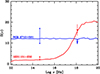 |
Fig. 7. Optical and X-ray degrees of polarization of the two sources. For the optical band, the bar indicate the range of measured values. The curves show two realization of the stratified shock scenario described in the text. |
Although the above model can satisfactorily reproduce the data, it is based on highly idealized and simplified hypotheses. Using dedicated magnetohydrodynamics (MHD) simulations, Sciaccaluga et al. (2025) show that this simple model can be adapted to a realistic scenario, considering the shocks produced in an underpressured jet recollimated by the external medium (Komissarov & Falle 1997). The model reproduces the commonly observed chromaticity of the polarization. However, the study also shows that the polarization properties, particularly the chromaticity, depend on the specific details of the system. In particular, the ratio of the poloidal to toroidal components of the helical magnetic field of the jet (i.e., the pitch) has a great impact. Interestingly, when the toroidal field dominates, the model produces reversed chromaticity, i.e., the degree of polarization decreases with frequency. This behavior is mainly dictated by asymmetries in the complex Doppler-boosting pattern of radiation from the flow downstream of the recollimation shock. These asymmetries are more pronounced at low frequencies (Sciaccaluga et al. 2025), as emitting electrons extend over a larger region. However, X-ray emission is produced in a compact region just after the shock, where boosting is much more uniform. These results suggest that the reversed chromaticity of RGB J0710+591 is related to a toroidal field larger than that typically found in the jet of other blazars.
4.2. Other scenarios
It is also interesting to compare the case of RGB J0710+591 with the alternative model proposed by Bolis et al. (2024). In this model, chromaticity is not related to the energy stratification of the emission region but rather arises naturally from the geometry of the fields. Assuming a field structure self-consistently calculated in the theory of force-free, Poynting-dominated jet, Bolis et al. (2024) show that the observed chromaticity arises when electrons occupy the same region and the jet has a parabolic shape. The increase of polarization with frequency is a robust feature of this model; therefore, the results for RGB J0710+591 are challenging to interpret without additional assumptions (for instance, multiple emission regions).
An alternative approach, motivated by the standard model for jet production and acceleration (e.g. Komissarov et al. 2009), assumes that emitting particles are energized through magnetic reconnection, which is thought to be more efficient than shock acceleration when the plasma is highly magnetized (Sironi et al. 2015). Both MHD simulations of magnetic reconnection triggered by kink instability in highly magnetized jets (Bodo et al. 2021) or Particle-In-Cell (PIC) simulations of single current sheaths (Zhang et al. 2020) display highly variable polarization (and flux) at both optical and X-ray energies, with a comparable averaged degree of polarization. However, a scenario based on these results appears incompatible with EHBL phenomenology, particularly with the small level of variability characterizing these sources (Biteau et al. 2020) and the small magnetization inferred from modeling the SED (Tavecchio & Ghisellini 2016).
These results highlight the complexity of the polarimetric properties of synchrotron emission from blazars and the need for good simultaneous multiwavelength coverage extending from radio to X-rays. We also emphasize the importance of refined models capable of capturing the complexity of the phenomenology displayed by these sources, including the polarimetric channel.
Acknowledgments
We acknowledge financial support from a INAF Theory Grant 2024 (PI F. Tavecchio). This work has been funded by the European Union-Next Generation EU, PRIN 2022 RFF M4C21.1 (2022C9TNNX). We acknowledge financial support from ASI grant I/004/11/6. We thank Dr. Brad Cenko and the Swift team for approving and carrying out the Swift ToO observations. Part of this work is based on archival data provided by the Space Science Data Center-ASI. The IAA-CSIC co-authors acknowledge financial support from the Spanish “Ministerio de Ciencia e Innovación” (MCIN/AEI/ 10.13039/501100011033) through the Center of Excellence Severo Ochoa award for the Instituto de Astrofísica de Andalucía-CSIC (CEX2021-001131-S), and through grants PID2019-107847RB-C44 and PID2022-139117NB-C44. Some of the data are based on observations collected at the Observatorio de Sierra Nevada; which is owned and operated by the Instituto de Astrofísica de Andalucía (IAA-CSIC), and at the Centro Astronómico Hispano en Andalucía (CAHA); which is operated jointly by Junta de Andalucía and Consejo Superior de Investigaciones Científicas (IAA-CSIC). The Submillimeter Array is a joint project between the Smithsonian Astrophysical Observatory and the Academia Sinica Institute of Astronomy and Astrophysics and is funded by the Smithsonian Institution and the Academia Sinica. Maunakea, the location of the SMA, is a culturally important site for the indigenous Hawaiian people; we are privileged to study the cosmos from its summit. E.L. was supported by Academy of Finland projects 317636 and 320045. P.K. was supported by Academy of Finland projects 346071 and 345899. P.K. acknowledges support from the Metsähovi Radio Observatory of Aalto University. This work was supported by JST, the establishment of university fellowships towards the creation of science technology innovation, Grant Number JPMJFS2129. This work was supported by Japan Society for the Promotion of Science (JSPS) KAKENHI Grant Numbers JP21H01137. This work was also partially supported by Optical and Near-Infrared Astronomy Inter-University Cooperation Program from the Ministry of Education, Culture, Sports, Science and Technology (MEXT) of Japan. We are grateful to the observation and operating members of Kanata Telescope. I.L was funded by the European Union ERC-2022-STG – BOOTES – 101076343. Views and opinions expressed are however those of the author(s) only and do not necessarily reflect those of the European Union or the European Research Council Executive Agency. Neither the European Union nor the granting authority can be held responsible for them. The data in this study include observations made with the Nordic Optical Telescope, owned in collaboration by the University of Turku and Aarhus University, and operated jointly by Aarhus University, the University of Turku and the University of Oslo, representing Denmark, Finland and Norway, the University of Iceland and Stockholm University at the Observatorio del Roque de los Muchachos, La Palma, Spain, of the Instituto de Astrofisica de Canarias. The data presented here were obtained in part with ALFOSC, which is provided by the Instituto de Astrofísica de Andalucía (IAA) under a joint agreement with the University of Copenhagen and NOT. We acknowledge funding to support our NOT observations from the Finnish Centre for Astronomy with ESO (FINCA), University of Turku, Finland (Academy of Finland grant nr 306531). This research was partially supported by the Bulgarian National Science Fund of the Ministry of Education and Science under grants KP-06-H68/4 (2022), KP-06-H78/5 (2023) and KP-06-H88/4 (2024). Partly based on observations with the 100-m telescope of the MPIfR (Max-Planck-Institut für Radioastronomie) at Effelsberg. Observations with the 100-m radio telescope at Effelsberg have received funding from the European Union’s Horizon 2020 research and innovation programme under grant agreement No 101004719 (ORP). F.E., S.H., J.H., M.K., and F.R. acknowledge support from the Deutsche Forschungsgemeinschaft (DFG, grants 447572188, 434448349, 465409577). G. F. P. acknowledges support by the European Research Council advanced grant “M2FINDERS – Mapping Magnetic Fields with INterferometry Down to Event hoRizon Scales” (Grant No. 101018682). C.C. acknowledges support from the European Research Council (ERC) under the Horizon ERC Grants 2021 programme under grant agreement No. 101040021.
References
- Aharonian, F. A., Khangulyan, D., & Costamante, L. 2008, MNRAS, 387, 1206 [NASA ADS] [CrossRef] [Google Scholar]
- Akitaya, H., Moritani, Y., Ui, T., et al. 2014, SPIE Conf. Ser., 9147, 91474O [NASA ADS] [Google Scholar]
- Angelakis, E., Hovatta, T., Blinov, D., et al. 2016, MNRAS, 463, 3365 [NASA ADS] [CrossRef] [Google Scholar]
- Arnaud, K. A. 1996, ASP Conf. Ser., 101, 17 [Google Scholar]
- Bachev, R. 2024, Bulg. Astron. J., 40, 78 [Google Scholar]
- Baldini, L., Bucciantini, N., Lalla, N. D., et al. 2022, SoftwareX, 19, 101194 [NASA ADS] [CrossRef] [Google Scholar]
- Benke, P., Rösch, F., Ros, E., et al. 2024, A&A, 681, A69 [NASA ADS] [CrossRef] [EDP Sciences] [Google Scholar]
- Biteau, J., Prandini, E., Costamante, L., et al. 2020, Nat. Astron., 4, 124 [Google Scholar]
- Blandford, R., & Eichler, D. 1987, Phys. Rep., 154, 1 [Google Scholar]
- Blandford, R., Meier, D., & Readhead, A. 2019, ARA&A, 57, 467 [NASA ADS] [CrossRef] [Google Scholar]
- Bodo, G., Tavecchio, F., & Sironi, L. 2021, MNRAS, 501, 2836 [NASA ADS] [CrossRef] [Google Scholar]
- Bolis, F., Sobacchi, E., & Tavecchio, F. 2024, A&A, 690, A14 [NASA ADS] [CrossRef] [EDP Sciences] [Google Scholar]
- Bonnoli, G., Tavecchio, F., Ghisellini, G., & Sbarrato, T. 2015, MNRAS, 451, 611 [NASA ADS] [CrossRef] [Google Scholar]
- Böttcher, M., Dermer, C. D., & Finke, J. D. 2008, ApJ, 679, L9 [CrossRef] [Google Scholar]
- Burrows, D. N., Hill, J. E., Nousek, J. A., et al. 2005, Space Sci. Rev., 120, 165 [Google Scholar]
- Capecchiacci, S., Liodakis, I., Middei, R., et al. 2025, arXiv e-prints [arXiv:2508.14168] [Google Scholar]
- Cash, W. 1979, ApJ, 228, 939 [Google Scholar]
- Cerruti, M. 2020, Galaxies, 8, 72 [NASA ADS] [CrossRef] [Google Scholar]
- Chang, J. S., & Cooper, G. 1970, J. Comput. Phys., 6, 1 [Google Scholar]
- Chiaberge, M., & Ghisellini, G. 1999, MNRAS, 306, 551 [Google Scholar]
- Costamante, L., Ghisellini, G., Giommi, P., et al. 2001, A&A, 371, 512 [NASA ADS] [CrossRef] [EDP Sciences] [Google Scholar]
- Costamante, L., Bonnoli, G., Tavecchio, F., et al. 2018, MNRAS, 477, 4257 [NASA ADS] [CrossRef] [Google Scholar]
- Del Zanna, L., Volpi, D., Amato, E., & Bucciantini, N. 2006, A&A, 453, 621 [NASA ADS] [CrossRef] [EDP Sciences] [Google Scholar]
- Di Gesu, L., Donnarumma, I., Tavecchio, F., et al. 2022, ApJ, 938, L7 [CrossRef] [Google Scholar]
- Di Marco, A., Costa, E., Muleri, F., et al. 2022, AJ, 163, 170 [NASA ADS] [CrossRef] [Google Scholar]
- Ehlert, S. R., Liodakis, I., Middei, R., et al. 2023, ApJ, 959, 61 [NASA ADS] [CrossRef] [Google Scholar]
- Eppel, F., Kadler, M., Heßdörfer, J., et al. 2024, A&A, 684, A11 [NASA ADS] [CrossRef] [EDP Sciences] [Google Scholar]
- Errando, M., Liodakis, I., Marscher, A. P., et al. 2024, ApJ, 963, 5 [NASA ADS] [CrossRef] [Google Scholar]
- Escudero Pedrosa, J., Agudo, I., Morcuende, D., et al. 2024a, AJ, 168, 84 [Google Scholar]
- Escudero Pedrosa, J., Morcuende Parrilla, D., & Otero-Santos, J. 2024b, https://doi.org/10.5281/zenodo.10222722 [Google Scholar]
- Falomo, R., & Ulrich, M. H. 2000, A&A, 357, 91 [Google Scholar]
- Fossati, G., Maraschi, L., Celotti, A., Comastri, A., & Ghisellini, G. 1998, MNRAS, 299, 433 [Google Scholar]
- HI4PI Collaboration (Ben Bekhti, N., et al.) 2016, A&A, 594, A116 [NASA ADS] [CrossRef] [EDP Sciences] [Google Scholar]
- Hovatta, T., Lindfors, E., Blinov, D., et al. 2016, A&A, 596, A78 [NASA ADS] [CrossRef] [EDP Sciences] [Google Scholar]
- Katarzyński, K., Ghisellini, G., Tavecchio, F., Gracia, J., & Maraschi, L. 2006, MNRAS, 368, L52 [Google Scholar]
- Kawabata, K. S., Okazaki, A., Akitaya, H., et al. 1999, PASP, 111, 898 [NASA ADS] [CrossRef] [Google Scholar]
- Kim, D. E., Di Gesu, L., Liodakis, I., et al. 2024a, A&A, 681, A12 [NASA ADS] [CrossRef] [EDP Sciences] [Google Scholar]
- Kim, D. E., Di Gesu, L., Marin, F., et al. 2024b, Galaxies, 12, 20 [Google Scholar]
- Kislat, F., Clark, B., Beilicke, M., & Krawczynski, H. 2015, Astropart. Phys., 68, 45 [NASA ADS] [CrossRef] [Google Scholar]
- Komissarov, S. S., & Falle, S. A. E. G. 1997, MNRAS, 288, 833 [Google Scholar]
- Komissarov, S. S., Vlahakis, N., Königl, A., & Barkov, M. V. 2009, MNRAS, 394, 1182 [NASA ADS] [CrossRef] [Google Scholar]
- Kostrichkin, I. M., Plavin, A. V., Pushkarev, A. B., & Butuzova, M. S. 2025, MNRAS, 537, 978 [Google Scholar]
- Kouch, P. M., Liodakis, I., Middei, R., et al. 2024, A&A, 689, A119 [NASA ADS] [CrossRef] [EDP Sciences] [Google Scholar]
- Kraus, A., Krichbaum, T. P., Wegner, R., et al. 2003, A&A, 401, 161 [NASA ADS] [CrossRef] [EDP Sciences] [Google Scholar]
- Lefa, E., Rieger, F. M., & Aharonian, F. 2011, ApJ, 740, 64 [NASA ADS] [CrossRef] [Google Scholar]
- Lemoine, M. 2013, MNRAS, 428, 845 [NASA ADS] [CrossRef] [Google Scholar]
- Liodakis, I., Marscher, A. P., Agudo, I., et al. 2022, Nature, 611, 677 [CrossRef] [Google Scholar]
- Lyutikov, M., Pariev, V. I., & Gabuzda, D. C. 2005, MNRAS, 360, 869 [Google Scholar]
- Marscher, A. P., & Gear, W. K. 1985, ApJ, 298, 114 [Google Scholar]
- Marscher, A. P., & Jorstad, S. G. 2022, Universe, 8, 644 [NASA ADS] [CrossRef] [Google Scholar]
- Marscher, A. P., Di Gesu, L., Jorstad, S. G., et al. 2024, Galaxies, 12, 50 [NASA ADS] [CrossRef] [Google Scholar]
- Massaro, E., Perri, M., Giommi, P., & Nesci, R. 2004, A&A, 413, 489 [NASA ADS] [CrossRef] [EDP Sciences] [Google Scholar]
- Matthews, J. H., Bell, A. R., & Blundell, K. M. 2020, New Astron. Rev., 89, 101543 [CrossRef] [Google Scholar]
- Myserlis, I., Angelakis, E., Kraus, A., et al. 2018, A&A, 609, A68 [NASA ADS] [CrossRef] [EDP Sciences] [Google Scholar]
- Myserlis, I., Agudo, I., Thum, C., et al. 2025, in Highlights of Spanish Astrophysics XII, eds. M. Manteiga, F. González-Galindo, A. Labiano-Ortega, et al., 121 [Google Scholar]
- Nilsson, K., Pasanen, M., Takalo, L. O., et al. 2007, A&A, 475, 199 [NASA ADS] [CrossRef] [EDP Sciences] [Google Scholar]
- Nilsson, K., Lindfors, E., Takalo, L. O., et al. 2018, A&A, 620, A185 [NASA ADS] [CrossRef] [EDP Sciences] [Google Scholar]
- Otero-Santos, J., Piirola, V., Escudero Pedrosa, J., et al. 2024, AJ, 167, 137 [Google Scholar]
- Planck Collaboration VI. 2020, A&A, 641, A6 [NASA ADS] [CrossRef] [EDP Sciences] [Google Scholar]
- Plavin, A. V., Kovalev, Y. Y., & Pushkarev, A. B. 2022, ApJS, 260, 4 [NASA ADS] [CrossRef] [Google Scholar]
- Romero, G. E., Boettcher, M., Markoff, S., & Tavecchio, F. 2017, Space Sci. Rev., 207, 5 [NASA ADS] [CrossRef] [Google Scholar]
- Sciaccaluga, A., & Tavecchio, F. 2022, MNRAS, 517, 2502 [NASA ADS] [CrossRef] [Google Scholar]
- Sciaccaluga, A., Costa, A., Tavecchio, F., et al. 2025, A&A, 699, A296 [NASA ADS] [CrossRef] [EDP Sciences] [Google Scholar]
- Sironi, L., Petropoulou, M., & Giannios, D. 2015, MNRAS, 450, 183 [Google Scholar]
- Sol, H., & Zech, A. 2022, Galaxies, 10, 105 [NASA ADS] [CrossRef] [Google Scholar]
- Strohmayer, T. E. 2017, ApJ, 838, 72 [NASA ADS] [CrossRef] [Google Scholar]
- Tavecchio, F. 2021, Galaxies, 9, 37 [NASA ADS] [CrossRef] [Google Scholar]
- Tavecchio, F., & Ghisellini, G. 2016, MNRAS, 456, 2374 [Google Scholar]
- Tavecchio, F., Ghisellini, G., Ghirlanda, G., Costamante, L., & Franceschini, A. 2009, MNRAS, 399, L59 [CrossRef] [Google Scholar]
- Tavecchio, F., Landoni, M., Sironi, L., & Coppi, P. 2018, MNRAS, 480, 2872 [NASA ADS] [CrossRef] [Google Scholar]
- Tavecchio, F., Costa, A., & Sciaccaluga, A. 2022, MNRAS, 517, L16 [NASA ADS] [CrossRef] [Google Scholar]
- Willingale, R., Starling, R. L. C., Beardmore, A. P., Tanvir, N. R., & O’Brien, P. T. 2013, MNRAS, 431, 394 [Google Scholar]
- Wilms, J., Allen, A., & McCray, R. 2000, ApJ, 542, 914 [Google Scholar]
- Wu, Z., Jiang, D. R., & Gu, M. 2012, MNRAS, 424, 2733 [Google Scholar]
- Zech, A., & Lemoine, M. 2021, A&A, 654, A96 [NASA ADS] [CrossRef] [EDP Sciences] [Google Scholar]
- Zhang, H., Li, X., Giannios, D., et al. 2020, ApJ, 901, 149 [CrossRef] [Google Scholar]
While obtained for a specific class of sources, these results are likely also valid for other kinds of astrophysical objects that host relativistic jets.
However, when the IXPE observation is split into four time bins, the third one yields a significant detection with ΠX = 7.5 (Errando et al. 2024).
The most extreme chromaticity is shown by PKS 2155-304, with ΠX/ΠO ≃ 7.2 (Kouch et al. 2024).
Appendix A: An improved stratified shock model
In this Appendix we briefly sketch the model that we have used to reproduce the multiwavelength polarimetric data of the two sources.
A.1. The model
The model improves the original scenario described in Tavecchio et al. (2018). In the following we highlight the main modifications.
The model assumes that relativistic electrons are injected at the front of a mildly relativistic shock normal to the jet axis, with downstream velocity (in the shock frame) βd, sh ≃ 1/3 which propagates in a cold cylindrical jet with radius rj.
The upstream jet flow is supposed to carry a weak field almost parallel to the jet axis with intensity B∥. A magnetic field with lines forming a small angle with respect to the shock normal (a configuration called a “parallel" shock) is prerequisite to have an efficient particle acceleration (e.g. Sironi et al. 2015). Kinetic simulations show the formation of an intense field parallel to the shock, self-generated by streaming accelerating particles, slowly decaying with distance in the downstream flow. Following Lemoine (2013), for definiteness we assume that the intensity of the generated field decays along the jet flow following a phenomenological power law:
 (A.1)
(A.1)
where d is the distance in the downstream measured from the shock and the power law index m is in the range 0.2 − 0.5. With this parametrization, λ plays the role of an effective decay length. Furthermore, we account for the micro-turbulent nature of the self-generated magnetic field by using a cell structure, each cell representing a coherence domain. At each point of the grid of d, we model ncells = 5 × 10³ equal cells assumed to uniformly fill the jet cross section (we checked that with a larger number of cells the results do not change). In each cell we specify the total magnetic field as the sum of the constant parallel field B∥ = Bz and the orthogonal field B⊥(d) (evaluated at distance of the cell from the shock, d), with components Bx, By, which we randomly select in each cell under the condition Bx2 + By2 = B⊥2(d). The simulation reported in Tavecchio et al. (2018) suggests that B⊥, 0/B∥ ≲ 10.
Relativistic electrons accelerated at the shock are advected downstream by the flow, experiencing radiative losses due to the emission of synchrotron and IC radiation. Tavecchio et al. (2018) used a simplified analytical treatment of the radiative cooling of the electrons. Here we adopt a self-consistent calculation of the electron energy distribution (i.e. numerical density of electrons with Lorentz factor in the range γ − γ + dγ ) at different distances from the shock, N(γ, d), by numerically solving the continuity equation including radiative losses, treated as in Chiaberge & Ghisellini (1999) using the robust fully implicit numerical scheme of Chang & Cooper (1970).
In the shock rest frame emitting (and cooling) particles are advected downstream with velocity vadv = βd, shc = c/3 (up to a distance dmax, where we assume the emission is quenched by jet expansion/adiabatic losses, e.g.,Marscher & Gear 1985). Therefore, we associated t to a distance d = vadvt from the shock. The distribution at time t (and distance vadvt) is thus provided by the solution of:
![Mathematical equation: $$ \begin{aligned} \frac{\partial N(\gamma ,t)}{\partial t} = \frac{\partial }{\partial \gamma } \left[ \dot{\gamma }_c(\gamma ,t) N(\gamma ,t)\right] + Q(\gamma ) \delta (t), \end{aligned} $$](/articles/aa/full_html/2026/05/aa58716-25/aa58716-25-eq10.gif) (A.2)
(A.2)
where  is the cooling rate, given by:
![Mathematical equation: $$ \begin{aligned} \dot{\gamma }_c= \frac{4}{3} \frac{\sigma _T c}{m_e c^2} [ U_B(d)+U_{\rm rad}] \gamma ^2, \end{aligned} $$](/articles/aa/full_html/2026/05/aa58716-25/aa58716-25-eq12.gif) (A.3)
(A.3)
where σT is the Thomson cross section, UB(d) is the (total) magnetic field energy density at distance d and Urad is the energy density of the radiation field. For simplicity, in the calculations we assume that only synchrotron losses are relevant (i.e. we fix Urad = 0) and we also neglect possible adiabatic and escape losses. We also neglect possible stochastic reacceleration/heating of electrons caused by interaction with turbulent fields in the post-shock flow (inferred to be of small intensity, Marscher & Jorstad 2022).
We assume that relativistic electrons, instantaneously injected at the shock at t = 0, follow a cut-offed power law energy distribution Q(γ)∝γ−nexp(−γ/γcut), with index n and minimum and cut-off Lorentz factor γmin and γcut.
In stationary conditions (suitable to model the quiescent state of the source during the observations analyzed here) the polarization can be calculated summing the Stokes parameters associated to each cell. In detail, Stokes parameters for each cell i as a function of the frequency in the observer frame, Uν, i, Qν, i and Iν, i, are calculated following the standard formalism (Lyutikov et al. 2005; Del Zanna et al. 2006). Finally, the total observed degree of polarization, Πν, and the electron vector position angle (EVPA), χν, are derived from the total Stokes parameters Uν = ∑Uν, i, Qν = ∑Qν, i and Iν = ∑Iν, i, by using the standard formulae:
 (A.4)
(A.4)
 (A.5)
(A.5)
A.2. Application to 1ES 1101-232 and RGB J0710+591
We reproduce the multiwavelength polarimetric data of the two sources adjusting the free parameters of the model. For both sources we fix the radius rj = 4 × 1015 cm, the poloidal field intensity Bz = 0.03 G, the normalization of the self-generated field B⊥, 0 = 0.25 G, the bulk Lorentz factor Γ = 20. Electrons are injected with a slope n = 2.1 with γcut = 106. The only different parameters for the two cases are the decay length and the slope of the self-produced field, λ and m, and the viewing angle, θv, that we report in Tab. A.1.
Parameters of the models.
The main difference concerns the details of the profile of the self-generated field. In particular, the small m used for RGB J0710+591 implies that the self generated field is important in the entire emission volume. With this configuration, when the jet is observed at small angle (θv < 1/Γ) the degree of polarization is independent of the frequency. This is shown in Fig.A.1, which shows Π(ν) for different observing angles.
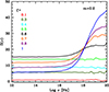 |
Fig. A.1. Degree of polarization as a function of frequency for different values of ζ in the range 0–1, keeping fixed the value of the Doppler factor, for parameters of model 1. |
The critical quantity determining the observed (projected) structure of the magnetic field, and thus the resulting polarization, is the observing angle as measured in the jet frame,  . For small (observer frame) viewing angles, suitable to the sources considered here, it is useful to consider the parameter ζ = Γθv, the product of the bulk Lorentz factor of the emitting plasma and the observer-frame viewing angle. In particular, ζ = 1 (i.e. θv = 1/Γ) corresponds to an observing angle in the downstream frame
  . In this situation, in the X-ray band one expects a rather large polarization, ideally close to the theoretical limit, since the region of emission is produced by the self-produced field whose projection is observed perfectly orthogonal to the jet axis. On the other hand, for decreasing values of the jet-frame viewing angles, the observer has access to both projected (random distributed) Bx and By components and this results in a lower degree of polarization. In the limiting case ζ → 0 (which corresponds to
  ) the effective polarization approaches zero at all frequencies, since the observer is located exactly along the jet axis and sees an equal contribution of the two (randomly distributed) components of the self produced field, Bx and By. Fig. A.1, reporting Πν for various values of ζ in the interval 0-1 clearly shows these effects.
Fig. A.2 instead illustrates the role of the decay length, λ, in shaping the degree of polarization (for the parameters used for RGB J0710+591). For very short λ (< 1013 cm) the self-genererated field decays very quickly and most of the low energy radiation (below the soft X-ray band) is produced in a volume where the field is dominated by the poloidal component, thus determining a high degree of polarization. For larger values of λ, the toroidal self-generated field is relevant in a large portion of the downstream volume, determining the decrease of the polarization fraction at lower frequencies (where both field components are important).
 |
Fig. A.2. Degree of polarization as a function of frequency for different values of λ, keeping fixed the value of the Doppler factor, for parameters of model 1. |
All Tables
Best-fit parameters from the spectropolarimetric analyses of 1ES 1101-232 and RGB J0710+591.
Best-fit parameters from the joint spectropolarimetric analyses of 1ES 1101-232 and RGB J0710+591.
All Figures
|
Fig. 1. Detection significance of X-ray polarization for 1ES 1101-232 (left) and RGB J0710+591 (right), as measured from the spectropolarimetric analysis. The tangential direction indicates the polarization angle, and the radial direction corresponds to the polarization degree. The colored dot at the center of each contour denotes the measured X-ray polarization. Contours correspond to detection confidence levels of 68%, 90%, and 99%. |
| In the text | |
|
Fig. 2. Light curve of the IXPE observation of RGB J0710+591. The green and orange shaded areas indicate periods one and two, respectively, split according to the central observation gap. The central dashed green line represents the average count rate of RGB J0710+591 during the IXPE observation. |
| In the text | |
|
Fig. 3. Joint spectropolarimetric analysis of 1ES 1101-232. Left: Energy flux spectra, expressed as photon flux multiplied by energy squared, for the Swift (red), IXPE I (yellow), and NuSTAR (blue) data together with the corresponding data-model residuals. The black line indicates the best-fit model. Right: IXPE Q and U spectra, displayed in green and orange, respectively, together with their deviations from the best-fit model. |
| In the text | |
|
Fig. 4. Joint spectropolarimetric analysis of RGB J0710+591. The panels follow the same format as in Figure 3. |
| In the text | |
|
Fig. 5. Optical polarization observations of RGB J0710+591. Top: Brightness in different optical bands. Middle: R-band polarization degree. Bottom: Polarization angle. The gray shaded area marks the duration of the IXPE observation, and the horizontal green band marks the jet direction as projected on the sky. |
| In the text | |
|
Fig. 6. Optical polarization observations of 1ES 1101-232. Panels and symbols are as in Fig. 5. The R-band† measurements (purple symbols) have not been corrected for the host-galaxy contribution. |
| In the text | |
|
Fig. 7. Optical and X-ray degrees of polarization of the two sources. For the optical band, the bar indicate the range of measured values. The curves show two realization of the stratified shock scenario described in the text. |
| In the text | |
|
Fig. A.1. Degree of polarization as a function of frequency for different values of ζ in the range 0–1, keeping fixed the value of the Doppler factor, for parameters of model 1. |
| In the text | |
|
Fig. A.2. Degree of polarization as a function of frequency for different values of λ, keeping fixed the value of the Doppler factor, for parameters of model 1. |
| In the text | |
Current usage metrics show cumulative count of Article Views (full-text article views including HTML views, PDF and ePub downloads, according to the available data) and Abstracts Views on Vision4Press platform.
Data correspond to usage on the plateform after 2015. The current usage metrics is available 48-96 hours after online publication and is updated daily on week days.
Initial download of the metrics may take a while.