| Issue |
A&A
Volume 709, May 2026
|
|
|---|---|---|
| Article Number | A183 | |
| Number of page(s) | 12 | |
| Section | Extragalactic astronomy | |
| DOI | https://doi.org/10.1051/0004-6361/202558644 | |
| Published online | 13 May 2026 | |
The undetectable fraction of core-collapse supernovae in luminous infrared galaxies
II. GSAOI/GeMS dataset
1
Tuorla Observatory, Department of Physics and Astronomy, University of Turku, 20014 Turku, Finland
2
School of Sciences, European University Cyprus, Diogenes street, Engomi, 1516 Nicosia, Cyprus
3
School of Mathematical and Physical Sciences, Macquarie University, Sydney, NSW 2109, Australia
4
Astrophysics and Space Technologies Research Centre, Macquarie University, Sydney, NSW 2109, Australia
5
Cosmic Dawn Center (DAWN)
6
Niels Bohr Institute, University of Copenhagen, Jagtvej 128, 2200 Kóbenhavn N, Denmark
7
Finnish Centre for Astronomy with ESO (FINCA), University of Turku, 20014 Turku, Finland
8
South African Astronomical Observatory, P.O. Box 9, Observatory, 7935 Cape Town, South Africa
★ Corresponding author: This email address is being protected from spambots. You need JavaScript enabled to view it.
Received:
18
December
2025
Accepted:
3
April
2026
Abstract
Context. Core-collapse supernovae (CCSNe) in luminous infrared galaxies (LIRGs) can have extreme line-of-sight host galaxy dust extinctions, which leads to a large fraction of the events remaining undetected by optical and infrared surveys. This population of undetected CCSNe is important to constrain in order to determine the cosmic CCSN rates, which can be used to estimate the cosmic star formation history independently from methods based on galaxy luminosities.
Aims. Our aim is to confirm and refine our estimates for the undetectable fraction of CCSNe in LIRGs in the local Universe. Our study is based on the near-infrared K-band multi-epoch SUNBIRD survey monitoring dataset of a sample of nine LIRGs using the Gemini-South telescope with the multi-conjugate GSAOI/GeMS laser guide star adaptive optics system.
Methods. We determined the limiting magnitudes for CCSN detection for each epoch in our dataset with artificial supernova injection and image subtraction methods. Subsequently, we used a Monte Carlo method to determine the combined effects of limiting magnitudes, survey cadence, CCSN subtype distribution, and their light curve evolution diversity. The intrinsic CCSN rates of the sample galaxies were estimated based on detailed modelling of their spectral energy distribution. Finally, we combined the resulting CCSN detection probabilities with the intrinsic CCSN rates for the dataset, and compared that against the real CCSN detections over the survey period.
Results. Based on our GSAOI/GeMS dataset, assuming optical or near-infrared example surveys with capabilities to detect CCSNe in local LIRGs with host extinctions of AV = 3 or 16 mag, respectively, the resulting total undetectable fractions are 86.0+4.7−5.9% and 53.6+15.6−19.6%. When folding in the results from our previous near-infrared adaptive optics assisted LIRG monitoring dataset, the corresponding total undetectable fractions are 88.3+2.6−3.2% and 61.4+8.5−10.6%, respectively.
Key words: supernovae: general / dust / extinction / galaxies: star formation
© The Authors 2026
 Open Access article, published by EDP Sciences, under the terms of the Creative Commons Attribution License (https://creativecommons.org/licenses/by/4.0), which permits unrestricted use, distribution, and reproduction in any medium, provided the original work is properly cited.
This article is published in open access under the Subscribe to Open model. This email address is being protected from spambots. You need JavaScript enabled to view it. to support open access publication.
1. Introduction
Core-collapse supernovae (CCSNe) are the terminal explosions at the end of the lifetime of massive stars above ∼8 M⊙ (e.g., Smartt 2009). Due to their relatively short lifespans, CCSNe can be used to trace the star formation rate (SFR). Estimating the SFR from the CCSN rate (SFRC) is a method independent from the usual luminosity-based methods (SFRL). There has been an ongoing discussion whether the SFRC and the SFRL agree at different redshift ranges. Horiuchi et al. (2011) noted a discrepancy between the reported SFRC and SFRL values, with the latter being roughly two times larger than the former at 0 < z < 0.4. This was challenged by Cappellaro et al. (2015), who found the SFRC and SFRL to be in agreements within errors for 0.05 < z < 0.35. Botticella et al. (2012) noted that the choice of the observational wavelength region in determining the SFRL has a large impact; for example, SFRs determined from Hα were found to be lower by a factor of about two compared to SFRs determined from far ultraviolet (FUV). Similarly Strolger et al. (2015) found a difference in SFRL obtained from UV plus IR observations and IR-only observations, with the UV plus IR derived SFRL matching the SFRC. Gruppioni et al. (2020) comprehensively collated different SFR estimates obtained through various approaches. The estimates are in good agreement at low z, but rapidly diverge after z ≈ 1. This is expected to some extent due to the inherent difficulties in observing at larger redshifts and is further enhanced by the increased contribution of dust-obscured star formation at higher redshifts (Magnelli et al. 2011; Zavala et al. 2021). In particular, CCSNe that remain undetected by surveys due to dust-obscuration have a major effect on the SFRC estimate (Mattila et al. 2012).
Luminous infrared galaxies (LIRGs) are defined as galaxies with 1011 L⊙ ≤ LIR < 1012 L⊙. The dominant source of the infrared luminosity is the reprocessing of UV and optical photons by dust and gas (Kennicutt 1998; Pérez-Torres et al. 2021). The source of the high-energy photons is hot young stars, active galactic nuclei (AGNs), or a combination of both. Luminous infrared galaxies are often in the process of merging or show signs of past interaction. Star formation in LIRGs is concentrated in the nuclear and circumnuclear regions at ∼0.1 to ∼1 kpc scales (Soifer et al. 2001), which results in a substantial fraction of CCSNe remaining undetected due to extinction and insufficient spatial resolution (Kool et al. 2018). While relatively rare in the local Universe, the contribution of LIRGs to the cosmic SFR becomes more significant at higher redshifts. At z = 1 the contribution of LIRGs to the total SFR at that redshift exceeds 50% (Magnelli et al. 2009). Thus, the study of cosmic SFR beyond the local Universe with CCSNe requires detailed understanding of these events in LIRGs.
Mattila et al. (2012) found that the fraction of undetected CCSNe in LIRGs by optical surveys can be as high as  . This result was based on 14 years of reported observations of the LIRG Arp 299 by various transient surveys, where the estimated intrinsic CCSN rate was compared to the number of detected events. Miluzio et al. (2013) found that by shifting a supernova (SN) survey to the K-band (where the extinction in flux is only ∼10−4 of optical) ∼60 to 75% of the CCSNe in LIRGs are not detected. Their result was based on detection efficiencies of artificial SNe simulated on the sample galaxies. Fox et al. (2021) used the Spitzer Space Telescope at 3.6 μm to survey high SFR galaxies for CCSNe. Despite the advantages of a space-based telescope operating in the near-IR, their results suggest that ∼83% of CCSNe remained undetected at < 150 Mpc. This likely resulted from the complex point spread function (PSF) of Spitzer data, resulting in poor detection efficiency in the central regions of galaxies, where most of the CCSNe explode. Mäntynen et al. (2025; hereafter Paper I) find that
  % and
% and  % of CCSNe in LIRGs in the local Universe are not detected by near-IR (assuming an extinction threshold of AV = 16 mag) and optical (AV = 3 mag) surveys, respectively. The result is based on adaptive optics (AO) monitoring of a sample of eight LIRGs using the Gemini-North telescope.
While the reduced impact of host extinction with infrared observations is quite effective compared to optical observations, a higher resolution is required to further lower the percentage of missed CCSNe. Kool et al. (2018) show that supplementing the advantages of the K-band with high angular resolution AO observations can decrease the fraction of undetected CCSNe in LIRGs, especially in the circumnuclear regions. Several CCSNe in central regions of LIRGs have been detected using this technique (e.g. Mattila et al. 2007; Kankare et al. 2008, 2012). Radio observations are unaffected by dust obscuration, and radio interferometry can reach extremely high angular resolutions. Unfortunately, only a fraction of CCSNe are bright enough in radio wavelengths to be readily detectable (e.g. Romero-Cañizales et al. 2014). Varenius et al. (2019) estimate that only ∼2.5 to ∼5.6% of CCSNe in the nearby ultraluminous infrared galaxy (ULIRG; 1012 L⊙ ≤ LIR ≤ 1013 L⊙) Arp 220 at 87 Mpc were detectable in radio. Thus, the high angular resolution surveys at near-IR bands provide the most comprehensive view of CCSNe in LIRGs, which in turn allows for a more accurate matching of SFRC and SFRL in the redshift regime, where most of the star formation is obscured by dust.
Studies of CCSN rates typically apply an extinction correction to their observed rates to take into account the effect of host extinction (e.g. Dahlen et al. 2012). However, extinction correction models for normal galaxies primarily suggest moderate obscuration and are not sufficient to explain the observed CCSN population in LIRGs, where the majority of these events can remain undetected. Furthermore, in addition to a population of CCSNe in LIRGs with host extinctions that could be described with a more obscured extinction correction model, there is a population of CCSNe in these galaxies with extremely high host extinctions, which remain undetected in all optical or infrared observations; this population is called the missing fraction (Mattila et al. 2012). The CCSNe within the missing fraction explode deep in their host galaxies in or behind dusty molecular clouds, primarily in the central regions of LIRGs. Mattila & Meikle (2001) measured extinctions of 19 SN remnants from the nearby starburst galaxy M 82 in the central 500 pc region based on H I and H2 column density measurements. This resulted in a mean extinction of AV = 24 ± 9 mag. Contrasting this with an example model of host extinction distribution for normal spiral galaxies by Riello & Patat (2005), excluding edge-on cases, the mean extinction barely reaches AV = 0.5 mag. Unfortunately, there is no host extinction model for CCSNe in LIRGs that would be based on a large number of SNe. However, in Paper I an extinction correction was derived based on a sample of 19 CCSNe in LIRGs (Kankare et al. 2021), which we adopted in our analysis.
Classical CCSN classification divides the SNe into hydrogen-rich Type II and hydrogen-poor Type I (also known as stripped-envelope SNe) based on their spectra. H-poor SNe are divided into Types IIb, Ib, and Ic. Spectroscopically they show progressively increased levels of envelope stripping, respectively showing some hydrogen, helium but no hydrogen, and neither hydrogen nor helium. Additionally, many subtypes can be further spectroscopically classified into narrow, broad-line, and peculiar subtypes. For example, Type IIn SNe are H-rich events that show narrow spectral lines (≲1000 km s−1). SN 1987A-like events are peculiar Type II SNe that resemble the historical SN 1987A, with a distinctive slowly rising light curve.
Here we build upon the results from Paper I by including observations conducted with the Gemini South telescope. Our methodology is the same as in Paper I: We performed a standard data reduction (Sect. 2), carried out algorithmically optimised template image subtraction (Sect. 3.1), determined the limiting magnitudes of the dataset via artificial SN injection (Sect. 3.2), and used a Monte Carlo simulation to determine the effects of different CCSN subtypes, peak magnitude variation, evolution timescale variability, host extinction, and survey cadence to produce CCSN detection probabilities for the dataset (Sect. 3.3). Finally, the intrinsic CCSN rates for the dataset were obtained via spectral energy distribution (SED) analysis through Markov Chains (SATMC). These were compared against the real detected CCSNe in the dataset to determine the missing fraction. Additionally, we estimated the fraction of CCSNe that remain undetected due to more moderate extinctions, in addition to the missing fraction. We calculated this fraction from a host extinction model. These two fractions form the total undetectable fraction. Results are summarised in Sect. 4, and we briefly discuss the implications of our results on the CCSN detectability at different redshifts in Sect. 5. Conclusions are provided in Sect. 6.
2. Dataset
The dataset used in this study was obtained by our Supernovae UNmasked By Infra-Red Detection (SUNBIRD) collaboration (Kool et al. 2018). The collaboration has used multiple AO programmes to discover and study CCSNe in LIRGs (e.g. Kankare et al. 2012, 2014) and characterise the super-star cluster population in these galaxies (e.g. Randriamanakoto et al. 2013, 2019, 2022).
The dataset in this analysis consists of 32 epochs in total from nine different LIRGs, from January 2013 to July 2017 (see Table 1 and Fig. 1). The sample includes galaxies up to a distance of 115 Mpc, with the LIRGs and the discovered CCSNe presented in the survey paper by Kool et al. (2018). The data were obtained using the Gemini-South telescope with the Gemini South Adaptive Optics Imager (GSAOI, 0.02″/pixel; McGregor et al. 2004; Carrasco et al. 2012), utilising the Gemini Multi-conjugate Adaptive Optics System (GeMS) in the K-band. The system uses five laser guide stars and ideally three natural guide stars to provide an effective and uniform AO correction over the 120″ × GSAOI field of view. The SUNBIRD observations were obtained with the programme IDs GS-2012B-SV-407, GS-2013A-Q-9, GS-2013B-Q-65, GS-2015A-C-2, GS-2015A-Q-6, GS-2015A-Q-7 (PI: Ryder), and GS-2016A-C-1 (PI: Kool). Furthermore, we complemented the analysis with archival data obtained with programme IDs GS-2014A-Q-21 (PI: Lai), GS-2014B-C-1 (PI: Sharp), GS-2015A-C-2 (PI: Sweet), and GS-2016A-C-2 (PI: Sweet) of the sample galaxies with the same K-band AO setup and similar image depth. Four LIRGs (ESO 264-G057, ESO 491-G020, MCG +02-20-003, and NGC 1204) were observed only once with GSAOI/GeMS in the SUNBIRD programme and were not included in the analysis due to the lack of a template image of similar quality. Typical on-source exposure times of the dataset were 9 × 60 s; however, in some epochs a fraction of the frames in the sequence were excluded from the final stacked image of aligned exposures due to poor delivered image quality.
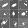 |
Fig. 1. Luminous infrared galaxies of the GSAOI/GeMS in 36″ × 36″ field of view (except NGC 3110 in 46″ × 46″). North is up, and east is to the left. Due to the pointing of the observations, the target galaxy is not necessarily in the centre of the shown image subsection. |
Summary of the dataset.
The flat field correction and sky subtraction steps were carried out with the Python based DRAGONS package (Labrie et al. 2023). No separate sky frames were taken for background subtraction and instead the background subtraction was carried out using a sky frame stacked from the individual dithered images. Alignment and co-addition of the reduced sequence images was performed based on the IRAF (Tody 1986) tasks geomap, geotran, and imcombine. The photometric calibration was based on the Two Micron All Sky Survey (2MASS; Skrutskie et al. 2006). The sample galaxy NGC 4575 had no 2MASS point sources in the reduced GSAOI/GeMS images and was therefore observed using the Nordic Optical Telescope (NOT; Djupvik & Andersen 2010) with the NOT near-infrared Camera and spectrograph (NOTCam) instrument via the NOT Unbiased Transient Survey 2 (NUTS2) programme. The NOTCam image was reduced using the external notcam package in IRAF, which included flat field correction, sky subtraction, and co-adding individual frames. The 2MASS calibrated NOT image was used to bootstrap magnitudes for several point sources in the GSAOI/GeMS images of NGC 4575. The aperture photometry was carried out using the Source Extractor program (Bertin & Arnouts 1996).
Four CCSNe were detected in the dataset: SN 2013if (Type IIP) in IRAS 18293-3413, SN 2015ca (Type IIP) in NGC 3110, SN 2015cb (Type II) in IRAS 17138-1017, and AT 2015cf (unclassified; see Sect. 3.4) in NGC 3110 (Kool et al. 2018). None of the detected transients were observed spectroscopically and the classifications were based on multi-band and multi-epoch photometry. This work did not discover any previously unreported transients in the GSAOI/GeMS dataset.
We obtained SEDs for seven LIRGs that had not been previously analysed for intrinsic CCSN rates similar to our previous study in Paper I. The LIRGs were: ESO 264-G036, ESO 267-G030, ESO 440-IG058, IRAS 08355-4944, NGC 3110, NGC 3508, and NGC 4575. The SEDs were constructed from a combination of archival photometry and spectra. The photometry was obtained from NASA/IPAC Extragalactic Database (NED) and included data from the Galaxy Evolution Explorer (GALEX, Seibert et al. 2012), the 2MASS programme, the wide-field Infrared Survey Explorer (WISE, Cutri et al. 2013), the Infrared Astronomical Satellite (IRAS, Sanders et al. 2003), the Herschel Space Observatory PACS/SPIRE (Chu et al. 2017), the Spitzer Space Telescope IRAC/MIPS (Capak et al. 2013), and the Submillimetre Common-User Bolometer Array (SCUBA, Dunne et al. 2000). Additional optical photometry by de Vaucouleurs et al. (1991) and Lauberts & Valentijn (1989) was also used. When choosing between multiple values for a given wavelength band, we chose the measurement with the largest aperture to best account for the flux from the whole LIRG. The Spitzer spectra were obtained from the Great Observatories All-sky LIRG Survey (GOALS) project (Armus et al. 2009) data access archive and were normalised to the photometry based on the 20 − 30 μm flux.
3. Method
Our method can be separated into four distinct parts: (1) automated constraining of optimal template subtraction parameters, (2) determining limiting magnitudes of the images via artificial CCSN injection, (3) deriving CCSN detection probabilities with a Monte Carlo method, and (4) yielding the undetected fraction by comparing the detection probabilities with the intrinsic CCSN rates derived via SED fitting for the dataset (3.3.4). Brief descriptions of these steps are presented in the following subsections. For a more detailed description, see Paper I.
3.1. Automatic image subtraction
We used the method described by James & Anderson (2006) to define the pixel regions covered by each sample LIRG in the GSAOI/GeMS images (hereafter galaxy maps). First, a median stacked image was created from the reduced and aligned images of a LIRG. The background level was subtracted from the median image. This level was a median value of a selected isolated area from the image, far from the LIRG and other field sources. Lastly, the pixel values were summed from the lowest to the highest. The ranked pixels before the sum reaches zero are considered to belong to the background, and the remaining to the LIRG or other field sources (e.g. foreground stars or unrelated galaxies). These other sources were excluded from the galaxy maps manually. The selection of the background sample area has some effect on the galaxy maps; however, the effect is limited to the faint outer edges of the LIRGs with a minimal contribution to our final results.
Template subtraction is a standard method used by SN search programs. The template subtraction in our study was performed with a modified version of the ISIS2.2 package (Alard & Lupton 1998; Alard 2000). In the process, two images are aligned, the image with narrower PSF is convolved to match the other image, and their flux levels are matched. Subsequently, one of the images is subtracted from the other pixel by pixel. Sources that remain constant between the image epochs (e.g. galaxies and stars) should disappear, and transient sources (e.g. CCSNe) should remain, given that the transient is not present in one of the images, or has sufficiently evolved between them. In practice, the subtraction process may leave residuals in the resulting image, particularly to the brightest regions in the images.
The template subtraction process is dependent on some of the chosen parameters (e.g. Melinder et al. 2012). With an aim to reduce the subjective human element, and to standardise the subtraction quality within the dataset, we developed an algorithm to semi-automatically perform the template subtraction as described in detail in Paper I. The user provides the code sets of initial guesses and permitted ranges for the parameters, which the code optimises. This algorithm was used to determine the sets of optimal template subtraction parameters for each image in the GSAOI/GeMS dataset to be used in the later steps. The quality of the subtraction was defined as the variance of the pixel values over the subtracted image in the galaxy map area, excluding the areas (stamps) used to derive the convolution kernel for the image subtraction process.
The stamp regions that were used for calculating the convolution kernel were not used in the analysis of the resulting subtracted images, since a possible faint transient in those areas would likely disappear in the process. Therefore, the subtraction process needs to be repeated at least twice to cover the whole image. In practice, multiple subtractions with different stamp combinations were performed to ensure that each cycle had sufficient coverage to derive the image convolution for the process.
3.2. Limiting magnitudes
Noise in the template subtracted images and residuals from the image subtraction process can have a major impact on the ability to recover transients from the resulting images. These effects are more prominent in regions with higher flux and stronger gradients (e.g. the LIRG nuclei or bright super star clusters). Thus, the recoverability of objects can greatly vary across the image, and spatially resolved estimates for the limiting magnitudes are required.
The code for this process was created in Paper I, and the GSAOI/GeMS dataset was analysed with the same approach. The method was to create artificial SNe with the IRAF routine mkobjects at different brightness levels in the images, carry out template subtraction process, and attempt to recover the simulated sources. The FWHM of the artificial SNe (Moffat profile parameter 2.5) was matched with the FWHM of the narrow core of the AO PSF of point sources in the original images.
The positions of the artificial SNe were determined by dividing the image into a grid with a spacing equal to the FWHM of that epoch. An artificial SN was created in the grid location if at least one galaxy map pixel was within it. Creating all these artificial SNe simultaneously would result in blending and render detecting them individually impossible. Therefore, the artificial SNe were created in groups, where they would be separated by at least seven times the FWHM of the image. This was found to be sufficient to prevent any notable overlap effect.
The following iterative process was used to determine the limiting magnitudes of an epoch. Artificial SNe with an apparent brightness of 16 mag were created on the image for which the image subtraction process was carried out. The artificial SNe were detected from the subtracted image with Source Extractor. The process was repeated with artificial SNe that were 0.2 mag fainter, and continued until no detections were made or the process had repeated 40 times. If there were areas where the starting brightness of 16 mag was not sufficient, these were re-analysed with a starting brightness of 14 mag. The threshold for a detection was set as a minimum of 9 pixels which are at least 5σ above the background level. Areas within 10 × FWHM of any previously detected real SNe in the dataset were excluded from the analysis. The minimum pixel count was chosen to exclude artefacts that cover only a few pixels in the subtracted images and are clearly not real. The conservative 5σ threshold was chosen by simulating sources at varying thresholds and choosing the limit at which the simulated sources were still readily detected by eye from the often noisy subtracted central regions of the sample galaxies.
Residuals from the subtraction process can cause false positives. This is further complicated when an artificial SN is created on or near an artefact. It becomes difficult to ascertain at which point the combined artificial SN and residual feature should no longer be counted as a detection. In these cases, the region was conservatively set as an undetectable region. This effect was mitigated by multiple subtractions with different sets of image subtraction stamps. The process described produces multiple sets of parameters for each epoch. The iterative process was performed for each of these. This resulted in each pixel in the galaxy map to have at least one limiting magnitude value. In cases where two or more values existed, the faintest magnitude limit was adopted.
3.3. Monte Carlo method
Core-collapse supernovae remain undetected in surveys due to a combination of factors: low cadence, insufficient imaging depth and resolution, poor image subtraction performance in nuclear regions, or high host extinction. Disentangling the effect of host extinction is not straightforward; however, we aimed to constrain this by simulating the SUNBIRD GSAOI/GeMS survey with varying degrees of extreme dust obscuration using a Monte Carlo method. Subsequently, we matched the expected CCSN detections of the simulation to the real detections from the dataset to derive the missing fraction and the undetectable fraction. The process was developed in Paper I, which also contains a more detailed description of the process.
The components of the Monte Carlo simulation were the survey cadence, detection thresholds for the faintest detectable CCSNe in each pixel in each epoch of the dataset, CCSN light curve templates and their variability ranges, host extinction model, the relative rates of CCSN subtypes, and the estimated intrinsic CCSN rates for the sample galaxies.
The time resolution of the simulation was one day, spatial resolution one pixel, and each run simulated 107 SNe. The following procedure was used. First, a CCSN subtype was chosen. Then an explosion date was randomly chosen within the typical detection window (i.e. control time; see Sect. 3.3.3). Then an explosion location was chosen from the galaxy map randomly with the probability directly proportional to the host galaxy K-band flux. Next, the light curve template was generated, and a host extinction, a galactic extinction, and a distance modulus were applied. The resulting apparent magnitude was then compared against the limiting magnitude of the explosion site pixel in the first epoch where the SN would be observable. If the SN was brighter, it was counted as a detection.
3.3.1. Template light curves
The subtypes of CCSNe considered in this work are: Ib, Ic, IIb, II, IIn, and SN 1987A-like. Similar to Paper I, the relative rates of these CCSN subtypes were adopted from the observed volume limited results of the Lick Observatory Supernova Search (LOSS, Li et al. 2000) with the CCSN classifications revised by Shivvers et al. (2017). This work adopts the CCSN peak magnitudes and their relative rates with small modifications. We combined the subtypes Type II-P and II-L into one population of Type II SNe. Similarly, the peculiar subtypes (e.g. Type IIb-peculiar) were combined with their respective non-peculiar subtypes. The narrow and broad line subtypes other than the Type IIn were also combined with their respective normal subtypes.
We created CCSN subtype light curve templates to be used in the Monte Carlo simulation in Paper I and briefly explain the process here. We chose a high quality K-band light curve of a CCSN for each subtype, that is a good representative of that subtype. The peak magnitudes of the templates are based on statistics of the optical LOSS sample revised by Shivvers et al. (2017) from which the K-band peak magnitudes were estimated based on R-K colour ranges adopted for different CCSN subtypes in Paper I.
To emulate the time-scale variability of CCSNe, we applied a time factor to the Type II and the stripped envelope templates. Similar to Paper I, we scaled the plateau phase of the template light curve to match the mean of the Anderson et al. (2014) sample and set the time factor range to match the variance of that sample. The time factor is then applied to the template plateau phase when the templates are generated in the simulation. A similar approach was taken with the stripped envelope template, except instead of the plateau length, the difference in magnitude between the peak and 15 days after the peak (mΔ15, Phillips 1993) was used to scale the photospheric phase of the light curve. The shortest possible time factor was restricted to match the fastest evolving SN in the colour comparison sample to exclude unphysically rapidly evolving templates. The time factor was applied to the first 35 days of the template to avoid unrealistic late-phase evolution. The adopted parameters for the CCSN subtype templates and ranges for their light curve variability are listed in table 1 of Paper I. The most likely templates of each CCSN subtype are presented in Fig. 2.
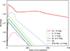 |
Fig. 2. Template K-band light curves of CCSN subtypes used in the Monte Carlo simulation. The light curves have been shifted vertically for clarity. The magnitudes are in the Vega system. |
3.3.2. Host extinction
Galactic extinction values were obtained from NED, which are based on the dust map calibration of Schlafly & Finkbeiner (2011). These are presented in Table 1. Kankare et al. (2021) reported host extinction estimates of 19 CCSNe discovered via optical or IR methods in the central regions of LIRGs with mean and median values of AV = 3.6 and 2.1 mag, respectively, which included the highest measured host extinction for an IR detected CCSN with an AV = 16 mag (Kankare et al. 2008). Furthermore, central regions of LIRGs can have extinctions of several hundreds of AV, with some up to AV ≫ 1000 mag (Pérez-Torres et al. 2021). For comparison, Pessi et al. (2023) measured host extinctions for 71 CCSNe in normal galaxies from the All-Sky Automated Survey for Supernovae (ASAS-SN, Shappee et al. 2014; Kochanek et al. 2017), resulting in mean values of AV = 0.23 ± 0.18 and 0.30 ± 0.16 mag for Type II and stripped envelope subtypes, respectively. It is clear that especially the optical observations are extremely biased towards lower extinctions and can only probe the surface layers of the LIRGs. We address this by dividing the CCSNe into two populations by their host extinctions, a surface component and a deep component.
The CCSN sample by Kankare et al. (2021) was used to describe the surface extinction component. The data were fit with an exponential function P(AV) = 0.881e−0.084AV with a median value of AV = 7.7 mag in Paper I. This extinction model is evaluated up to AV = 40 mag, which roughly corresponds to the most highly extinguished CCSN that could reasonably be detected in the dataset. The simulated CCSNe were randomly assigned host extinctions from this distribution.
The deep component describes the population of CCSNe that explode deep in the dusty clouds in the central regions of the LIRGs and is completely undetectable with optical and IR surveys. We refer to this as the missing fraction. Each run of the Monte Carlo simulation had a set probability for any simulated CCSN to be assigned in the missing fraction, which was varied between subsequent runs from 0 to 99%.
3.3.3. Control time
Transient surveys with a more limited cadence may have SNe explode and fade below the detection limit before the next survey epoch. This results in the effective survey time being shorter than the survey duration bound by the first and the last epochs, and should be accounted for when calculating the expected SN rates. Likewise, simulating SN explosions on epochs where the time to the next survey observations is too long introduces a bias towards a lower missing fraction. Therefore, in our Monte Carlo method, the simulated CCSNe can only explode during time windows where the time to the next epoch is within the control time (CT) of that CCSN subtype for that LIRG, including before the first epoch. CT is a measure of how long a SN could be typically detected, and is dependent on the SN subtype and the survey depth (see e.g. Cappellaro et al. 1993).
Our method of calculating the CT for a given CCSN subtype and epoch was the following: 105 light curves were randomly generated based on the parameters introduced in Sect. 3.3.1. The distance modulus and random host extinction were applied as described in Sect. 3.3.2. The CT was calculated as the mean time the light curves remain above a magnitude limit. The magnitude limit was a weighted average of the magnitude limits of an epoch (Sect. 3.2), where the weight was proportional to the flux of that pixel relative to the total flux of the galaxy. This was repeated for all CCSN subtypes and for all epochs. The CTs for the sample galaxies are listed in Tables A.1–A.9 in the Appendix. The median CT of the fastest evolving CCSN template IIb was 109 days.
Total control time (TCT) is a measure of the effective survey time for a galaxy. It is calculated as the sum of times between epochs, except when the CT corresponding to the latter epoch is shorter than the time between epochs. The TCT is used to calculate the underlying CCSN count for each of the CCSN subtypes.
3.3.4. Intrinsic CCSN rates
We estimated intrinsic CCSN rates for the LIRGs in the dataset with an adapted version of the SATMC Monte Carlo code (Johnson et al. 2013; Efstathiou et al. 2022). SATMC method fits several components to the SED of the sample LIRGs to determine their relative contributions. The components were as follows: starburst (Efstathiou et al. 2000; Efstathiou & Siebenmorgen 2009), AGN (Efstathiou & Rowan-Robinson 1995; Efstathiou et al. 2013), and a spheroidal galaxy (Efstathiou et al. 2021) or a disc galaxy (Efstathiou et al. 2022). The SED of the starburst component determines the age of the starburst episode, which was allowed to range within 5–50 Myr. The starburst model incorporates the stellar population synthesis model of Bruzual & Charlot (1993; 2003) which combined with the luminosity can estimate the mass of stars that formed in the starburst episode and the resulting CCSN rate based on the age of the starburst and its e-folding time, which was allowed to range within 1–40 Myr. The method adopts the Salpeter IMF for both the starburst and spheroidal components. The starburst model assumes solar metallicity, whereas the spheroidal component assumes that the metallicity is 40% of solar. The same approach was also used in Paper I.
In this work, we derived the inferred intrinsic CCSN rates for ESO 264-G036, ESO 267-G030, ESO 440-IG058, IRAS 08355-4944, NGC 3110, NGC 3508, and NGC 4575. The intrinsic CCSN rates for IRAS 17138-1017, and IRAS 18293-3413 were obtained from Kankare et al. (2021) and derived with the identical method. The estimated intrinsic CCSN rates are summarised in Table 1, and the SED fits are shown in Fig. 3.
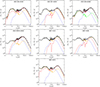 |
Fig. 3. Results of the SED modelling (solid black) of seven LIRGs of the GSAOI/GeMS dataset produced in this work. The model components are: either a spheroidal (dot-dashed orange) or a disc (dot-dashed green) galaxy, starburst contribution (dashed red), and an AGN (dotted blue). |
3.3.5. Error estimation
In order to estimate the errors in the Monte Carlo method, we ran the code with various parameters offset by their respective errors. The parameters included and their respective errors were the following. Limiting magnitude determination used a 0.2 mag step size, resulting in an error of ±0.2 mag. To estimate the uncertainty of the photometric calibration, we measured the standard deviation of the photometric zero point corrections from epochs with the same total exposure time, and conservatively chose the largest one, resulting in an error of ±0.335 mag. This error estimation reflects the effects of varying AO correction effectiveness on the Strehl ratio. The increased flux in the unresolved PSF wings caused by less effective AO correction results in uncertainty in the photometric calibration. For the colour correction MR − MK in the CCSN peak magnitude distributions, we chose the largest standard deviation within a CCSN subtype. This was amongst H-poor templates, resulting in an error of ±0.26 mag (Paper I). Finally, the error in distance modulus was ±0.15 mag for all the sample LIRGs, reported by NED. Thus, the resulting total error as the square root of the sum of squares is ±0.49 mag. Additionally, we applied Poissonian confidence limits by Gehrels (1986) to the inferred small number of intrinsic CCSNe in the simulation to address the small number statistics, which dominates the uncertainty in the resulting undetectable fractions of CCSNe in LIRGs.
3.4. The nature of AT 2015cf in NGC 3110
The GSAOI/GeMS follow-up dataset of AT 2015cf reported by Kool et al. (2018) is limited to two epochs of K-band detections at mK = 20.97 ± 0.13 and 21.4 ± 0.2 mag on JD 2457092.6 and JD 2457172.4, respectively, and two H and J-band limits of mH > 22.7 mag and mJ > 22.8 mag on JD 2457174.4. The two epochs or detections confirm that the transient is real; however, based on such a small amount of data the nature of the event remained ambiguous. The K-band data points suggest a decline rate of γK = 0.54 ± 0.30 mag (100 d)−1, which is slower than the theoretical 0.98 mag (100 d)−1 decline rate of the 56Co to 56Fe decay tail assuming a complete gamma-ray trapping where 56Co is a decay product of 56Ni synthesised in a SN explosion. If AT 2015cf is a CCSN, it is obscured by dust, intrinsically faint, and/or observed at late phases, based on the faint K-band detections and deep H and J-band limits. Unfortunately, there are no constraining pre-explosion limits for the event; thus it is plausible that the transient was discovered at a late-time epoch. While there are CCSNe discovered in the central regions of LIRGs with high derived host galaxy line-of-sight extinctions (e.g. SN 2008cs with  mag at a projected distance of 1.5 kpc; Kankare et al. 2008) the apparent location of AT 2015cf in one of the spiral arms of NGC 3110 is quite removed at a projected distance of 3.5 kpc. If not a CCSN, the most likely alternatives to consider for the origin of AT 2015cf are gap transients such as intermediate luminosity red transients (ILRTs) and luminous red novae (LRNe), which are red in colour and intrinsically fainter than most CCSNe (e.g. Pastorello & Fraser 2019).
The ILRT events have been suggested in the literature to be SNe where electron capture reactions of 24Mg or 20Ne in the O-Ne-Mg core of a low-mass massive star would trigger a terminal SN explosion rather than the core-collapse of an iron core (e.g. Cai et al. 2021). SN 2008S (e.g. Prieto et al. 2008; Botticella et al. 2009; Wanajo et al. 2009) is a prototypical member of these electron-capture SN candidates. The LRN transients have been associated in the literature with stellar merger powered common envelope events in close binary systems (e.g. Pastorello et al. 2019); thus, these events are likely not terminal explosions. These events are characterised by double-peaked light curves and are thought to be more massive versions of the classical Galactic red nova V1309 Sco (Tylenda et al. 2011). While fainter than typical CCSNe, the volumetric rate of SN 2008S-like ILRTs could be relatively high compared to the CCSN rate (up to ∼10%; Mattila et al. 2012). The rate of LRNe is more uncertain.
Unfortunately, well sampled late-time JHK-band light curves of CCSNe are rare in the literature. Kool et al. (2018) carried out a comparison of the observations of AT 2015cf to the near-IR evolution of representative examples of H-rich and H-poor SNe of the Type IIP SN 1999em (Krisciunas et al. 2009) and the Type IIb SN 2011dh (Ergon et al. 2014, 2015), respectively. With adjustments to the intrinsic brightness of the comparison events, the observational epoch, and the host galaxy extinction, contextual similarity to the observations of AT 2015cf can be achieved; however, in both cases the K-band brightness of these template events declines more rapidly than the observations of AT 2015cf. While the nature of AT 2015cf remained uncertain, Kool et al. (2018) favoured the H-rich CCSN origin for the event. Recently, late-time JHK-band observations have been reported in the literature for a variety of transients, which enabled us to carry out new χ2 comparisons to ILRTs, LRNe, and CCSNe. We highlight comparisons to the ILRT AT 2019abn (μ = 29.67 mag, AVtot = 1.936 mag; Valerin et al. 2025), the LRN AT 2021blu (μ = 29.68 mag, AVtot = 0.062 mag; Pastorello et al. 2023), and the Type IIP SN 2023ixf (μ = 29.17 mag, AVtot = 0.121 mag; Singh et al. 2024) in Fig. 4. In the case of SN 2023ixf the JHK-band light curves do not extend further than roughly 128 d from the approximate K-band peak; therefore, we linearly extrapolated the tail phase evolution with a linear fit. In all the comparisons, we do not adjust the intrinsic brightness of the events, and we assume no host extinction for AT 2015cf. In all these cases reasonable matches can be achieved assuming that the first detection of AT 2015cf took place within a 200 to 400 d range from the onset of the event. If AT 2015cf was reddened by some host galaxy extinction similar light curve matches would have been possible if AT 2015cf was detected somewhat earlier and/or the comparison events would have been intrinsically somewhat brighter. However, we note that AT 2019abn and AT 2021blu are located already in the bright end of the observed ILRT and LRN distributions, respectively.
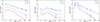 |
Fig. 4. Absolute light curves of AT 2015cf (with detections as points and limits with downwards pointing arrows) compared to a selection of events (curves) including the ILRT AT 2019abn (left), the LRN AT 2021blu (centre), and the Type IIP SN 2023ixf (right). The extrapolated tail phase of SN 2023ixf is indicated with dotted lines. The intrinsic brightness of the events has not been adjusted and no host galaxy extinction is assumed for AT 2015cf. |
Based on these comparisons, we favour the simplest explanation that AT 2015cf is a terminal SN explosion of an unconfirmed type. However, for completeness, we report the results for the missing and undetectable fractions for both cases of including and excluding AT 2015cf from the sample of SNe discovered in the GSAOI/GeMS monitoring programme of LIRGs; this does not have a major effect on our conclusions when the other uncertainties are taken into account.
4. Results
The output of a single run of the Monte Carlo simulation is an average detection probability for any CCSN subtype, for a given missing fraction and LIRG. We calculated the expected number of CCSNe in the dataset over the survey period (which excludes CCSNe that occur during survey gaps) based on the TCTs of the dataset and the intrinsic CCSN rates inferred based on the SED MCMC template fitting of the sample galaxies. By running the simulation with different missing fraction values we explored how the resulting estimated CCSN detection probabilities compare with the number of detected CCSNe. By multiplying the estimated intrinsic number of CCSNe with the different CCSN detection probabilities from the Monte Carlo simulation, we calculated the expected number of CCSN detections for each explored missing fraction value. Finally, we compared the number of expected CCSN detections to the number of real detections to constrain the missing fraction required to explain the discrepancy (see Fig. 5).
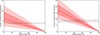 |
Fig. 5. Number of expected CCSN detections over the survey period of the dataset as a function of the missing fraction. Left: The GSAOI/GeMS dataset. Right: The GSAOI/GeMS dataset combined with the ALTAIR/NIRI dataset from Paper I. Red line: The mean value. Shaded red areas: 1σ and 2σ confidence intervals. Poissonian upper and lower limits due to small number statistics and the cumulative effect of other error sources are combined here. Dashed black: Number of real detected CCSNe in the survey(s). We note that while the expected CCSN counts for the datasets are 9 and 25 CCSNe for GSAOI/GeMS alone, and GSAOI/GeMS combined with ALTAIR/NIRI dataset, respectively, the Monte Carlo simulations result in detecting significantly less CCSNe even at 0% missing fraction. This is caused by a combined effect of faint CCSNe, moderate extinction and long time interval until the next observation epoch within the yielded CT. |
Because the CCSN nature of event AT 2015cf is uncertain, we calculate the missing fraction for both cases. Assuming that AT 2015cf was a genuine CCSN, based on the number of four detected CCSNe in the dataset, we obtain a missing fraction of  %. However, excluding the event AT 2015cf results in a missing fraction of
  %.
%.
Because the method used in Paper I is the same as in this work, we can reduce the effect of small number statistics by combining the results of this work with the results obtained in Paper I with Near-InfraRed Imager (NIRI; Hodapp et al. 2003) and the ALTtitude conjugate Adaptive optics for the InfraRed (ALTAIR). The combined dataset increased the number of expected CCSNe in the dataset from 16 to 25, reducing the Poissonian small number statistical error by ∼20% The combined dataset contains nine or eight (excluding AT 2015cf) detected CCSNe, which results in a missing fraction of  % or
% or  %, respectively. We note that because the width of the confidence intervals are dependent on the value of the missing fraction, the improvement in the statistics might not seem apparent.
The missing fraction of CCSNe in LIRGs represents the fraction of events that are undetectable by all optical and near-IR surveys due to the extreme host extinctions. In addition to the missing fraction, CCSNe remain undetected due to more moderate host extinctions. We estimate that fraction by integrating the host extinction model (Sect. 3.3.2) from infinity to a set of extinction thresholds. For example, assuming an optically discovered CCSN with the highest host extinction from Kankare et al. (2021) as the extinction threshold with AV ≈ 3 mag, integrating the host extinction results in 78% remaining undetected within the surface extinction distribution. After this fraction is applied to the population of CCSNe not part of the missing fraction, we obtain a total undetectable fraction of  % based on the combined dataset with a total of nine CCSNe. The highest host extinction in the CCSN sample used to determine the host extinction model is AV = 16 mag. Taking this as an extinction threshold for K-band surveys, we obtain a total undetectable fraction of
  %. The total undetectable fractions for a sample of extinction thresholds and both datasets are presented in Table 2.
Total undetectable fractions calculated from the missing fraction and the extinction model.
Since the results between Paper I and this work are very similar, comparisons to previous work done in Paper I also apply here, summarised below. Miluzio et al. (2013) found a total fraction of ∼60% to 75% of CCSNe in LIRGs to remain undiscovered in K-band. Comparing this to our total undetectable fraction of K-band surveys we find them in good agreement. This is unsurprising since the observed wavelength and sample of galaxies are similar.
Mattila et al. (2012) found a missing fraction of  % for LIRGs with optical surveys assuming an extinction correction similar to that of normal galaxies; therefore, this result roughly corresponds to our derived undetectable fraction. Our estimate of undetectable fraction for optical surveys using AV = 3 mag as the threshold is well consistent with this value within errors; however, we do note that due to the error ranges we find agreeable undetectable fractions for threshold values between AV = 2 mag to AV ≈ 10 mag. Their result was based on a single frequently observed LIRG, Arp 299.
For completeness, we report the median CT of our fastest evolving template (Type IIb) as 109 days. Therefore, for a similar survey with a cadence of ∼100 days, one expects to have at least one detection for 50% of the detectable Type IIb SNe.
5. Discussion
The results derived in this work are based on LIRGs in the local Universe (median distance 84 Mpc; z = 0.018), and applying them to LIRGs at larger redshifts is not straightforward, in particular due to the evolution of this galaxy population. Magnelli et al. (2011) measured the contributions of normal galaxies and (U)LIRGs to the cosmic SFR density at 0.0 < z < 2.3, and found that LIRGs account for roughly 5, 35, 50, and 50% of the SFR density at redshifts of 0.0, 0.5, 1.0, and 2.0, respectively. The SFR density is traced by the CCSN rate, and assuming that our result of ∼90% undetectable fraction of CCSNe applies for LIRGs at all redshifts when probing the rest frame optical wavelengths, a major fraction of CCSNe remain undiscovered regardless of the survey depth beyond the local Universe. Thus, the undetectable fraction of CCSNe in LIRGs has a crucial effect on the observed cosmic CCSN rates and their usage as independent probes of the cosmic star formation history beyond the local Universe (see e.g. DeCoursey et al. 2025). Furthermore, Mattila et al. (2012) estimate that nearly 100% of CCSNe in the local ULIRGs are not detected by optical surveys. The contribution of ULIRGs to the SFR density increases with redshift, reaching ∼20% at z = 2 (Magnelli et al. 2011).
6. Conclusions
We have presented updated estimates for the fraction of CCSNe in LIRGs in the local Universe that remain undetected by SN surveys, with a detailed description of our method. The analysis in this work is based on the SUNBIRD survey near-IR K-band monitoring dataset of nine LIRGs using the Gemini-South telescope with the GSAOI/GeMS AO system. The survey detected four transients, of which three are photometrically classified as CCSNe, and one is tentatively a CCSN discovered at late times.
We present the total undetectable fractions based on the analysed dataset, which consist of the missing fraction, and an additional survey extinction threshold dependent fraction of CCSNe that remain undiscovered due to moderate extinctions. We present these for a selection of survey extinction thresholds, and highlight two cases of AV = 3 and 16 mag, which act as proxies for optical and near-IR surveys, respectively. Based on four CCSNe in the dataset, we find total undetectable fractions of  % and
% and  % for optical and near-IR surveys, respectively.
Finally, we present the aggregate results of this work combined with those from Paper I derived with the same method for the SUNBIRD ALTAIR/NIRI laser guide star AO dataset of a sample of nine LIRGs monitored using the Gemini-North telescope. We find a total undetectable fractions of  % and
% and  % for optical and near-IR surveys, respectively. The facilities such as the Vera C. Rubin Observatory and the James Webb Space Telescope will probe the intrinsic CCSN rates with an unprecedented accuracy, on which the undetectable fraction of CCSNe will have a crucial impact beyond the local Universe at higher redshifts dominated by (U)LIRGs.
Acknowledgments
We thank the anonymous referee for useful comments. IM, EK, and KM acknowledge financial support from the Emil Aaltonen foundation. TMR is part of the Cosmic Dawn Center (DAWN), which is funded by the Danish National Research Foundation under grant DNRF140. TMR and SM acknowledge support from the Research Council of Finland project 350458. Based on observations obtained at the international Gemini Observatory, a program of NSF NOIRLab, which is managed by the Association of Universities for Research in Astronomy (AURA) under a cooperative agreement with the U.S. National Science Foundation on behalf of the Gemini Observatory partnership: the U.S. National Science Foundation (United States), National Research Council (Canada), Agencia Nacional de Investigación y Desarrollo (Chile), Ministerio de Ciencia, Tecnología e Innovación (Argentina), Ministério da Ciência, Tecnologia, Inovações e Comunicações (Brazil), and Korea Astronomy and Space Science Institute (Republic of Korea). Based on observations made with the Nordic Optical Telescope, owned in collaboration by the University of Turku and Aarhus University, and operated jointly by Aarhus University, the University of Turku and the University of Oslo, representing Denmark, Finland and Norway, the University of Iceland and Stockholm University at the Observatorio del Roque de los Muchachos, La Palma, Spain, of the Instituto de Astrofisica de Canarias. Observations from the NOT were obtained through the NUTS2 collaboration which is supported in part by the Instrument Centre for Danish Astrophysics (IDA), and the Finnish Centre for Astronomy with ESO (FINCA) via Academy of Finland grant nr 306531. This publication makes use of data products from the Two Micron All Sky Survey, which is a joint project of the University of Massachusetts and the Infrared Processing and Analysis Center/California Institute of Technology, funded by the National Aeronautics and Space Administration and the National Science Foundation. This research has made use of the NASA/IPAC Extragalactic Database (NED), which is operated by the Jet Propulsion Laboratory, California Institute of Technology, under contract with the National Aeronautics and Space Administration. This research has made use of the NASA/IPAC Infrared Science Archive, which is funded by the National Aeronautics and Space Administration and operated by the California Institute of Technology.
References
- Alard, C. 2000, A&AS, 144, 363 [NASA ADS] [CrossRef] [EDP Sciences] [Google Scholar]
- Alard, C., & Lupton, R. H. 1998, ApJ, 503, 325 [Google Scholar]
- Anderson, J. P., González-Gaitán, S., Hamuy, M., et al. 2014, ApJ, 786, 67 [Google Scholar]
- Armus, L., Mazzarella, J. M., Evans, A. S., et al. 2009, PASP, 121, 559 [Google Scholar]
- Bertin, E., & Arnouts, S. 1996, A&AS, 117, 393 [NASA ADS] [CrossRef] [EDP Sciences] [Google Scholar]
- Botticella, M. T., Pastorello, A., Smartt, S. J., et al. 2009, MNRAS, 398, 1041 [NASA ADS] [CrossRef] [Google Scholar]
- Botticella, M. T., Smartt, S. J., Kennicutt, R. C., et al. 2012, A&A, 537, A132 [NASA ADS] [CrossRef] [EDP Sciences] [Google Scholar]
- Bruzual, A. G., & Charlot, S. 1993, ApJ, 405, 538 [NASA ADS] [CrossRef] [Google Scholar]
- Bruzual, G., & Charlot, S. 2003, MNRAS, 344, 1000 [NASA ADS] [CrossRef] [Google Scholar]
- Cai, Y. Z., Pastorello, A., Fraser, M., et al. 2021, A&A, 654, A157 [NASA ADS] [CrossRef] [EDP Sciences] [Google Scholar]
- Capak, P. L., Teplitz, H. I., Brooke, T. Y., Laher, R., & Science Center, S. 2013, AAS Meet. Abstr., 221, 340.06 [Google Scholar]
- Cappellaro, E., Turatto, M., Benetti, S., et al. 1993, A&A, 268, 472 [Google Scholar]
- Cappellaro, E., Botticella, M. T., Pignata, G., et al. 2015, A&A, 584, A62 [NASA ADS] [CrossRef] [EDP Sciences] [Google Scholar]
- Carrasco, E. R., Edwards, M. L., McGregor, P. J., et al. 2012, in Adaptive Optics Systems III, eds. B. L. Ellerbroek, E. Marchetti, & J. P. Véran (International Society for Optics and Photonics (SPIE)), 8447, 84470N [Google Scholar]
- Chu, J. K., Sanders, D. B., Larson, K. L., et al. 2017, ApJS, 229, 25 [Google Scholar]
- Cutri, R. M., Wright, E. L., Conrow, T., et al. 2013, Explanatory Supplement to the AllWISE Data Release Products, Explanatory Supplement to the AllWISE Data Release Products, by R. M. Cutri et al. [Google Scholar]
- Dahlen, T., Strolger, L.-G., Riess, A. G., et al. 2012, ApJ, 757, 70 [NASA ADS] [CrossRef] [Google Scholar]
- de Vaucouleurs, G., de Vaucouleurs, A., Corwin, H. G., Jr., et al. 1991, Third Reference Catalogue of Bright Galaxies [Google Scholar]
- DeCoursey, C., Egami, E., Pierel, J. D. R., et al. 2025, ApJ, 979, 250 [Google Scholar]
- Djupvik, A. A., & Andersen, J. 2010, Astrophys. Space Sci. Proc., 14, 211 [NASA ADS] [CrossRef] [Google Scholar]
- Dunne, L., Eales, S., Edmunds, M., et al. 2000, MNRAS, 315, 115 [Google Scholar]
- Efstathiou, A., & Rowan-Robinson, M. 1995, MNRAS, 273, 649 [Google Scholar]
- Efstathiou, A., & Siebenmorgen, R. 2009, A&A, 502, 541 [NASA ADS] [CrossRef] [EDP Sciences] [Google Scholar]
- Efstathiou, A., Rowan-Robinson, M., & Siebenmorgen, R. 2000, MNRAS, 313, 734 [Google Scholar]
- Efstathiou, A., Christopher, N., Verma, A., & Siebenmorgen, R. 2013, MNRAS, 436, 1873 [NASA ADS] [CrossRef] [Google Scholar]
- Efstathiou, A., Małek, K., Burgarella, D., et al. 2021, MNRAS, 503, L11 [Google Scholar]
- Efstathiou, A., Farrah, D., Afonso, J., et al. 2022, MNRAS, 512, 5183 [NASA ADS] [CrossRef] [Google Scholar]
- Ergon, M., Sollerman, J., Fraser, M., et al. 2014, A&A, 562, A17 [NASA ADS] [CrossRef] [EDP Sciences] [Google Scholar]
- Ergon, M., Jerkstrand, A., Sollerman, J., et al. 2015, A&A, 580, A142 [NASA ADS] [CrossRef] [EDP Sciences] [Google Scholar]
- Fox, O. D., Khandrika, H., Rubin, D., et al. 2021, MNRAS, 506, 4199 [NASA ADS] [CrossRef] [Google Scholar]
- Gehrels, N. 1986, ApJ, 303, 336 [Google Scholar]
- Gruppioni, C., Béthermin, M., Loiacono, F., et al. 2020, A&A, 643, A8 [NASA ADS] [CrossRef] [EDP Sciences] [Google Scholar]
- Hodapp, K. W., Jensen, J. B., Irwin, E. M., et al. 2003, PASP, 115, 1388 [Google Scholar]
- Horiuchi, S., Beacom, J. F., Kochanek, C. S., et al. 2011, ApJ, 738, 154 [NASA ADS] [CrossRef] [Google Scholar]
- James, P. A., & Anderson, J. P. 2006, A&A, 453, 57 [NASA ADS] [CrossRef] [EDP Sciences] [Google Scholar]
- Johnson, S. P., Wilson, G. W., Tang, Y., & Scott, K. S. 2013, MNRAS, 436, 2535 [Google Scholar]
- Kankare, E., Mattila, S., Ryder, S., et al. 2008, ApJ, 689, L97 [Google Scholar]
- Kankare, E., Mattila, S., Ryder, S., et al. 2012, ApJ, 744, L19 [Google Scholar]
- Kankare, E., Mattila, S., Ryder, S., et al. 2014, MNRAS, 440, 1052 [Google Scholar]
- Kankare, E., Efstathiou, A., Kotak, R., et al. 2021, A&A, 649, A134 [NASA ADS] [CrossRef] [EDP Sciences] [Google Scholar]
- Kennicutt, R. C. 1998, ARA&A, 36, 189 [NASA ADS] [CrossRef] [Google Scholar]
- Kochanek, C. S., Shappee, B. J., Stanek, K. Z., et al. 2017, PASP, 129, 104502 [Google Scholar]
- Kool, E. C., Ryder, S., Kankare, E., et al. 2018, MNRAS, 473, 5641 [Google Scholar]
- Krisciunas, K., Hamuy, M., Suntzeff, N. B., et al. 2009, AJ, 137, 34 [Google Scholar]
- Labrie, K., Simpson, C., Cardenes, R., et al. 2023, Res. Notes AAS, 7, 214 [Google Scholar]
- Lauberts, A., & Valentijn, E. A. 1989, The Surface Photometry Catalogue of the ESO-Uppsala Galaxies (Garching: European Southern Observatory) [Google Scholar]
- Li, W. D., Filippenko, A. V., Treffers, R. R., et al. 2000, AIP Conf. Ser., 522, 103 [Google Scholar]
- Magnelli, B., Elbaz, D., Chary, R. R., et al. 2009, A&A, 496, 57 [NASA ADS] [CrossRef] [EDP Sciences] [Google Scholar]
- Magnelli, B., Elbaz, D., Chary, R. R., et al. 2011, A&A, 528, A35 [NASA ADS] [CrossRef] [EDP Sciences] [Google Scholar]
- Mäntynen, I., Kankare, E., Mattila, S., et al. 2025, A&A, 700, A199 [NASA ADS] [CrossRef] [EDP Sciences] [Google Scholar]
- Mattila, S., & Meikle, W. P. S. 2001, MNRAS, 324, 325 [Google Scholar]
- Mattila, S., Väisänen, P., Farrah, D., et al. 2007, ApJ, 659, L9 [Google Scholar]
- Mattila, S., Dahlen, T., Efstathiou, A., et al. 2012, ApJ, 756, 111 [Google Scholar]
- McGregor, P., Hart, J., Stevanovic, D., et al. 2004, in Ground-based Instrumentation for Astronomy, eds. A. F. M. Moorwood, & M. Iye (International Society for Optics and Photonics (SPIE)), 5492, 1033 [Google Scholar]
- Melinder, J., Dahlen, T., Mencía Trinchant, L., et al. 2012, A&A, 545, A96 [NASA ADS] [CrossRef] [EDP Sciences] [Google Scholar]
- Miluzio, M., Cappellaro, E., Botticella, M. T., et al. 2013, A&A, 554, A127 [NASA ADS] [CrossRef] [EDP Sciences] [Google Scholar]
- Pastorello, A., & Fraser, M. 2019, Nat. Astron., 3, 676 [Google Scholar]
- Pastorello, A., Mason, E., Taubenberger, S., et al. 2019, A&A, 630, A75 [NASA ADS] [CrossRef] [EDP Sciences] [Google Scholar]
- Pastorello, A., Valerin, G., Fraser, M., et al. 2023, A&A, 671, A158 [NASA ADS] [CrossRef] [EDP Sciences] [Google Scholar]
- Pérez-Torres, M., Mattila, S., Alonso-Herrero, A., Aalto, S., & Efstathiou, A. 2021, A&ARv, 29, 2 [CrossRef] [Google Scholar]
- Pessi, T., Prieto, J. L., Anderson, J. P., et al. 2023, A&A, 677, A28 [NASA ADS] [CrossRef] [EDP Sciences] [Google Scholar]
- Phillips, M. M. 1993, ApJ, 413, L105 [Google Scholar]
- Prieto, J. L., Kistler, M. D., Thompson, T. A., et al. 2008, ApJ, 681, L9 [NASA ADS] [CrossRef] [Google Scholar]
- Randriamanakoto, Z., Väisänen, P., Ryder, S., et al. 2013, MNRAS, 431, 554 [Google Scholar]
- Randriamanakoto, Z., Väisänen, P., Ryder, S. D., & Ranaivomanana, P. 2019, MNRAS, 482, 2530 [NASA ADS] [CrossRef] [Google Scholar]
- Randriamanakoto, Z., Väisänen, P., Ranaivomanana, P., et al. 2022, MNRAS, 513, 4232 [Google Scholar]
- Riello, M., & Patat, F. 2005, MNRAS, 362, 671 [Google Scholar]
- Romero-Cañizales, C., Herrero-Illana, R., Pérez-Torres, M. A., et al. 2014, MNRAS, 440, 1067 [Google Scholar]
- Sanders, D. B., Mazzarella, J. M., Kim, D. C., Surace, J. A., & Soifer, B. T. 2003, AJ, 126, 1607 [Google Scholar]
- Schlafly, E. F., & Finkbeiner, D. P. 2011, ApJ, 737, 103 [Google Scholar]
- Seibert, M., Wyder, T., Neill, J., et al. 2012, AAS Meet. Abstr., 219, 340.01 [Google Scholar]
- Shappee, B. J., Prieto, J. L., Grupe, D., et al. 2014, ApJ, 788, 48 [Google Scholar]
- Shivvers, I., Modjaz, M., Zheng, W., et al. 2017, PASP, 129, 054201 [NASA ADS] [CrossRef] [Google Scholar]
- Singh, A., Teja, R. S., Moriya, T. J., et al. 2024, ApJ, 975, 132 [CrossRef] [Google Scholar]
- Skrutskie, M. F., Cutri, R. M., Stiening, R., et al. 2006, AJ, 131, 1163 [NASA ADS] [CrossRef] [Google Scholar]
- Smartt, S. J. 2009, ARA&A, 47, 63 [NASA ADS] [CrossRef] [Google Scholar]
- Soifer, B. T., Neugebauer, G., Matthews, K., et al. 2001, AJ, 122, 1213 [Google Scholar]
- Strolger, L.-G., Dahlen, T., Rodney, S. A., et al. 2015, ApJ, 813, 93 [NASA ADS] [CrossRef] [Google Scholar]
- Tody, D. 1986, SPIE Conf. Ser., 627, 733 [Google Scholar]
- Tylenda, R., Hajduk, M., Kamiński, T., et al. 2011, A&A, 528, A114 [NASA ADS] [CrossRef] [EDP Sciences] [Google Scholar]
- Valerin, G., Pastorello, A., Reguitti, A., et al. 2025, A&A, 695, A42 [NASA ADS] [CrossRef] [EDP Sciences] [Google Scholar]
- Varenius, E., Conway, J. E., Batejat, F., et al. 2019, A&A, 623, A173 [NASA ADS] [CrossRef] [EDP Sciences] [Google Scholar]
- Wanajo, S., Nomoto, K., Janka, H. T., Kitaura, F. S., & Müller, B. 2009, ApJ, 695, 208 [NASA ADS] [CrossRef] [Google Scholar]
- Zavala, J. A., Casey, C. M., Manning, S. M., et al. 2021, ApJ, 909, 165 [CrossRef] [Google Scholar]
Appendix A: Additional tables
Survey epochs and CTs of ESO 264-G036.
Survey epochs and CTs of ESO 267-G030.
Survey epochs and CTs of ESO 440-IG058.
Survey epochs and CTs of IRAS 08355-4944.
Survey epochs and CTs of IRAS 17138-1017.
Survey epochs and CTs of IRAS 18293-3413.
Survey epochs and CTs of NGC 3110.
Survey epochs and CTs of NGC 3508.
Survey epochs and CTs of NGC 4575.
All Tables
Total undetectable fractions calculated from the missing fraction and the extinction model.
All Figures
|
Fig. 1. Luminous infrared galaxies of the GSAOI/GeMS in 36″ × 36″ field of view (except NGC 3110 in 46″ × 46″). North is up, and east is to the left. Due to the pointing of the observations, the target galaxy is not necessarily in the centre of the shown image subsection. |
| In the text | |
|
Fig. 2. Template K-band light curves of CCSN subtypes used in the Monte Carlo simulation. The light curves have been shifted vertically for clarity. The magnitudes are in the Vega system. |
| In the text | |
|
Fig. 3. Results of the SED modelling (solid black) of seven LIRGs of the GSAOI/GeMS dataset produced in this work. The model components are: either a spheroidal (dot-dashed orange) or a disc (dot-dashed green) galaxy, starburst contribution (dashed red), and an AGN (dotted blue). |
| In the text | |
|
Fig. 4. Absolute light curves of AT 2015cf (with detections as points and limits with downwards pointing arrows) compared to a selection of events (curves) including the ILRT AT 2019abn (left), the LRN AT 2021blu (centre), and the Type IIP SN 2023ixf (right). The extrapolated tail phase of SN 2023ixf is indicated with dotted lines. The intrinsic brightness of the events has not been adjusted and no host galaxy extinction is assumed for AT 2015cf. |
| In the text | |
|
Fig. 5. Number of expected CCSN detections over the survey period of the dataset as a function of the missing fraction. Left: The GSAOI/GeMS dataset. Right: The GSAOI/GeMS dataset combined with the ALTAIR/NIRI dataset from Paper I. Red line: The mean value. Shaded red areas: 1σ and 2σ confidence intervals. Poissonian upper and lower limits due to small number statistics and the cumulative effect of other error sources are combined here. Dashed black: Number of real detected CCSNe in the survey(s). We note that while the expected CCSN counts for the datasets are 9 and 25 CCSNe for GSAOI/GeMS alone, and GSAOI/GeMS combined with ALTAIR/NIRI dataset, respectively, the Monte Carlo simulations result in detecting significantly less CCSNe even at 0% missing fraction. This is caused by a combined effect of faint CCSNe, moderate extinction and long time interval until the next observation epoch within the yielded CT. |
| In the text | |
Current usage metrics show cumulative count of Article Views (full-text article views including HTML views, PDF and ePub downloads, according to the available data) and Abstracts Views on Vision4Press platform.
Data correspond to usage on the plateform after 2015. The current usage metrics is available 48-96 hours after online publication and is updated daily on week days.
Initial download of the metrics may take a while.