| Issue |
A&A
Volume 709, May 2026
|
|
|---|---|---|
| Article Number | A159 | |
| Number of page(s) | 12 | |
| Section | Cosmology (including clusters of galaxies) | |
| DOI | https://doi.org/10.1051/0004-6361/202557357 | |
| Published online | 13 May 2026 | |
CosmoGen: A genetic algorithm framework for the exploration of dark energy dynamics
1
Instituto de Astrofísica e Ciências do Espaço, Faculdade de Ciências, Universidade de Lisboa, Tapada da Ajuda, PT-1349-018 Lisboa, Portugal
2
Departamento de Física, Faculdade de Ciências, Universidade de Lisboa, Edifício C8, Campo Grande, PT1749-016 Lisboa, Portugal
★ Corresponding author: This email address is being protected from spambots. You need JavaScript enabled to view it.
Received:
22
September
2025
Accepted:
11
March
2026
Abstract
Context. The standard Lambda cold dark matter (ΛCDM) paradigm of the physical Universe suffers from well-known conceptual problems and is challenged by observational data. Alternative models exist in the literature, both phenomenological and physically motivated, but many of them suffer from similar or new problems.
Aims. We propose a method to mechanically generate alternative models in a data-informed procedure tuned to mitigate specific problems.
Methods. We implemented a computational framework, dubbed CosmoGen, based on evolutionary algorithms for symbolic regression. The evolutionary process is guided by the computation of structure formation and background cosmological quantities. As a proof-of-concept, we applied the procedure to the specific case of dark energy fluid models and asked the framework to generate models capable of alleviating the cosmological tensions S8 and H0.
Results. The system generated models with high fitness values, and through a Bayesian analysis of an illustrative model, we show that the model indeed alleviates the tensions, even though the Bayes factor indicates a weaker preference for ΛCDM.
Key words: methods: numerical / cosmological parameters / dark energy / large-scale structure of Universe
© The Authors 2026
 Open Access article, published by EDP Sciences, under the terms of the Creative Commons Attribution License (https://creativecommons.org/licenses/by/4.0), which permits unrestricted use, distribution, and reproduction in any medium, provided the original work is properly cited.
This article is published in open access under the Subscribe to Open model. This email address is being protected from spambots. You need JavaScript enabled to view it. to support open access publication.
1. Introduction
A quarter of a century after its discovery (Riess et al. 1998; Perlmutter et al. 1999), the accelerated expansion of the Universe remains a central puzzle of modern cosmology. The cosmological constant, which can be included in the Einstein equations in a natural way, has been the standard way to account for the accelerated expansion, establishing the Lambda cold dark matter (ΛCDM) paradigm. Although this paradigm has been successful in explaining current observations of the Universe, it faces significant challenges, from the interpretation of the cosmological constant as the vacuum energy density (Weinberg 1989) to the coincidence problem (Zlatev et al. 1999) to the tensions between low- and high-redshift measurements of the Hubble constant and the S8 parameter (Planck Collaboration XVI 2014; Riess et al. 2016; Hildebrandt et al. 2017).
The theoretical investigation of dark energy alternatives to the cosmological constant as a source of accelerated expansion is a very active field of research, and there is a long list of proposed models of various types (Di Valentino et al. 2021). Since the early days of this puzzle, a programme of observational probes of dark energy was initiated (Albrecht et al. 2006). Through measurements of background-level and large-scale structure formation observables, ΛCDM was thoroughly tested and the viability of alternative models was assessed. We are currently at the start of the fourth stage of this programme. Recent results of the first of the stage-IV cosmological surveys, performed with the Dark Energy Spectroscopic Instrument (DESI), favour a dynamical dark energy (DESI Collaboration 2025). The first stage-IV space-based survey, ESA’s Euclid mission, started its 6-year nominal cosmological survey in 2024 (Euclid Collaboration: Mellier et al. 2025), and it will be followed by the ground-based Legacy survey of Space and Time (LSST) of the Vera C. Rubin observatory (LSST Science Collaboration 2009) and NASA’s Nancy Grace Roman Space Telescope (Roman ROTAC and CCSDC 2025). These surveys will provide unprecedented datasets in terms of the number of tracers, image resolution, number of filters, and spectroscopic resolving power and will be accompanied by improvements in the handling of systematics.
The traditional way to infer dark energy properties from data is to constrain the specific parameters of physical dark energy models against data or to constrain general features shared by various models such as the derivative of the equation of state of dark energy at a pivot point (Linder 2003). However, the vast amounts of data and improved likelihoods may also be used to guide the construction of the cosmological models themselves. Today, this approach is possible thanks to the new computational techniques introduced by machine learning (ML). This is the approach followed in this work, where we create phenomenological models by generating cosmological functions according to data features encoded in the likelihood. For this, we developed a framework that integrates ML techniques with a cosmology solver and parameter space sampling methods.
In computer science, ML is a field dedicated to developing methods and algorithms capable of learning from data to describe systems or perform specific tasks (Turing 1950; Carbonell et al. 1983). Based on the organisation and structure of the data, ML is generally divided into two primary subfields: supervised learning and unsupervised learning (Webb & Goode 2025). If the sample data are labelled, that is, each data point is associated with a known correct measurement, then it is a supervised learning problem. The purpose of Supervised learning is to develop a predictive model that forecasts the future behaviour of a system based on past observations. This process, also called fitting or training, involves adjusting model parameters to match the model closer to the observations. Common examples of supervised learning tasks include classification, regression, and time series modelling. If the data are unlabelled, it is an unsupervised learning problem, where the goal is to identify hidden patterns or structures within the data. Typical examples of unsupervised learning tasks include clustering and dimensionality reduction.
There are many applications of ML in physics, astronomy, and cosmology (see Carleo et al. 2019; Fluke & Jacobs 2020, Ntampaka et al. 2019, respectively, for reviews), and some of them have used symbolic regression, the ML technique we use in this work. Symbolic regression (Kronberger et al. 2024a) is a type of supervised learning optimised for regression problems. Today, the most used learning algorithms for symbolic regression are evolutionary algorithms inspired by principles of natural selection (Goldberg 1989; Haupt & Haupt 2004). The symbolic regression technique is capable of building functional forms by combining a set of operators, operands, and rules. Unlike classic regression techniques, which require predetermined functional forms, symbolic regression optimises the functional form, the order of operators, and the numerical parameters. Symbolic regression enables the exploration of a range of potential equations that best fit the data. Thus, a goal of symbolic regression is to discover ‘physical laws’ that can be analytically expressed from the data. As an example, symbolic regression has been successfully applied in rediscovering planetary motion laws using the trajectories of the Sun, planets, and major moons in the Solar System (Lemos et al. 2023).
Symbolic regression has been used in cosmology, for example, in studies of N-body simulations (Li et al. 2021), baryonic feedback (Wadekar et al. 2023), and enhanced models of halo occupation distribution (Delgado et al. 2022). More relevant for our goal, symbolic regression has also been used to generate cosmological functions (Arjona & Nesseris 2020; Koksbang 2023; Bartlett et al. 2024). Most studies that use symbolic regression to generate phenomenological cosmological functions guided by data rely only on background-level observables. In contrast, our framework CosmoGen uses both background and large-scale structure data, allowing the symbolic regression algorithms to explore the vast space of potential dark energy models.
The new framework, CosmoGen, integrates supervised learning symbolic regression methods with the cosmological Boltzmann code CLASS (Lesgourgues 2011; Blas et al. 2011) and the Bayesian inference tool MontePython (Audren et al. 2013; Brinckmann & Lesgourgues 2019). In this framework, each candidate model proposed by the symbolic regression algorithm is implemented on the fly as a modified version of CLASS, treating it as a new dark energy or dark matter component. MontePython then performs a preliminary parameter estimation using a likelihood tuned to the objectives to be achieved, and it returns a fitness score. The score is fed back into the evolutionary loop of the symbolic regression algorithm. This is a hybrid approach between traditional sampling methods and evolutionary strategies. The evolutionary methods are tasked with discovering functional forms, whereas the traditional sampling methods are responsible for evaluating each functional form and extracting the best-fit values for its parameters.
In Sect. 2, we introduce the evolutionary methods used by the ML part of the framework. In Section 3 we describe the CosmoGen framework, including its prototype implementation. In Sect. 4 the framework is applied to a case study, namely, the building of dark energy fluid models generated to alleviate the Hubble and S8 tensions. One model from the resulting population of generated models is selected and analysed in Sect. 5, where its parameters are constrained. We conclude our work in Sect. 6.
2. Evolutionary methods
Symbolic regression has been integrated into a wide number of evolutionary methods. These methods can be organised into the following categories (Kronberger et al. 2024a): regression-based divided in linear and non-linear methods, expression tree-based including genetic programming (GP; Koza 1992), reinforcement learning (Sutton & Barto 2018), and transformer neural networks (Vaswani et al. 2017). There are also many variants that include several combinations of these methods, such as AI-Feyman (Udrescu & Tegmark 2020), a physics-inspired method, and symbolic metamodel (Abroshan et al. 2023), a mathematics-inspired method.
Genetic programming (Koza 1992) is an evolutionary algorithm widely used in symbolic regression. In evolutionary algorithms, a population of solution candidates is used in a parallel search process. This approach involves repeatedly recombining, mutating, and evaluating portions of solution candidates to gradually achieve improvements. The algorithm simulates processes observed in natural evolution, particularly the inheritance of traits from parents to offspring and selection pressure. GP algorithms are tree-based expressions composed of primitives, for example, binary and unary operators such as multiplication or exponential, and terminals that represent the variables and constants used to formulate a function. These are defined in what is called a ‘PrimitiveSet’.
The GP algorithm proceeds as follows:
-
Initialisation: A population of solution candidates (referred to as individuals) is randomly generated.
-
Fitness evaluation: Each individual is evaluated based on a fitness function to measure its quality or how well it solves the problem.
-
While loop or Stopping criteria: The following steps are repeated until a predefined stopping criterion is met (e.g. a maximum number of generations or satisfactory fitness level):
-
Parent selection: A subset of individuals is chosen to be parents, typically based on their fitness values.
-
Recombination: New individuals (children) are generated from the selected parents through recombination or crossover, creating variations in the population.
-
Fitness evaluation of children: Each child is evaluated to determine its fitness.
-
Replacement: Based on their fitness values, individuals from the current population and from the set of new children are selected to form the next population.
-
-
Return the best individual: The algorithm outputs the best-performing individual from the population.
In this work we use GP as the evolutionary algorithm because of its simplicity in implementation. However, the method shows great inefficiency in the production of candidates. This is due to the fact that tree-based methods for a certain space of genotypes and for a specific tree length limit can generate multiple expressions that represent the same function (Kronberger et al. 2024b). Exhaustive symbolic regression (Bartlett et al. 2024) is an example of an alternative method that could be implemented on future versions of CosmoGen that addresses the inefficiency problems of GP in the context of cosmological model generation.
Evolutionary algorithms also need to handle a second problem, namely, overfitting. For this, the algorithms in general aim for a balance between an accurate fit and simple equations. Indeed, while more complex functions can achieve a higher accuracy on specific datasets, they tend to generalise poorly due to overfitting. Hence, limiting the model complexity is an important point since simpler and interpretable expressions, though not always the most accurate, frequently exhibit a more reliable extrapolation behaviour. Achieving this balance between accuracy and simplicity to derive the ‘best’ equation for a given dataset requires a procedure for managing these two aspects. This can be done by including a penalty for complex models in the fitness evaluation or, alternatively, (as done in this work) by applying an evolutionary strategy with a large initial population and a population of mixed generations at each iteration, which prevents a fast increase of model complexity.
3. CosmoGen framework
The CosmoGen framework contains two primary components: the ML component and the cosmological component. The ML component consists of a symbolic regression method, which is implemented via the Distributed Evolutionary Algorithms in Python (DEAP) package1. The DEAP is a framework for implementing evolutionary algorithms, including but not limited to GP. The cosmological component is linked to a modified version of CLASS.
The ML component focuses on building the structure of the cosmological equation, i.e. the functional form of the candidates. The choice of method used to generate a population of candidates can be adjusted with ease. Currently, the framework uses a standard tree-based GP from DEAP, with minimal modifications. The cosmological component evaluates the candidates for physical viability, integrating CLASS computations and MontePython sampling methods. This second component is integrated in the GP loop, acting on points two and three of the procedure outlined in Sect. 2.
The physical interpretation of each individual depends on the desired case study and is determined by how it is integrated into the modified version of CLASS. Our framework provides a wide range of possibilities for exploration. It allows the user to consider any new cosmological component for which the relevant cosmological equations for background and perturbations can be written in a generalised form.
Fixing the generalised equations provides the Ansatz for the new cosmological component. CosmoGen generates new candidates considering the specific Ansatz. Three modified versions of CLASS can be included in CosmoGen, allowing for three Ansaetze: one designed for the potential of scalar fields (which can represent either scalar field dark matter or dark energy), one for a cosmological fluid (which may be dark matter, dark energy, or unified dark matter-energy), and another to explore models with couplings between dark matter and dark energy. Only the cosmological fluid case is fully implemented in the current version of CosmoGen.
In the case study presented here, we consider a dark energy fluid ρDE(a) with no perturbations that will replace the cosmological constant in the standard ΛCDM model. This case is implemented by adding a new dark energy fluid instance to CLASS (and setting ΩΛ = 0.).
To run CosmoGen, the following components are required:
-
The DEAP package, which provides the evolutionary algorithms used for symbolic regression, along with other standard Python packages. These can be easily installed through Pip or Conda.
-
A compiled version of CLASS, which is used for cosmological computations.
-
The MontePython code, which is employed for the optimisation of the coefficients using Markov chain Monte Carlo (MCMC) methods.
CosmoGen contains an input file that defines the GP configuration for the simulation as well as the paths for CLASS, MontePython, and the simulation output. The code runs following the procedure described in Sects. 3.1 through 3.5, which is summarised in Fig. 1.
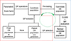 |
Fig. 1. Flowchart showing the sequence of steps of a CosmoGen run. The ML component is enclosed in the solid red border, and the cosmological component is within the dashed blue border. The sequence of steps moves through the two components in a loop. The terms ‘GP’ and ‘MP’ stand for GP and MontePython, respectively. See text for a full description. |
3.1. Initial population
The algorithm begins by randomly generating an initial population of candidates. This is done by applying a predefined set of operations (e.g. addition, multiplication, sine, logarithm, negation) to a predefined number of variables (e.g. the scale factor) and coefficients (free parameters to allow different coefficients on the various terms of the functional forms generated).
3.2. Pre-testing
The evolutionary process then starts from this first generation and continues in an iterative loop. Each step of the loop corresponds to one generation. In each iteration, the population passes through a pre-testing procedure that filters the individuals that have the potential to be a dark energy model. The pre-testing consists of the following steps applied to each individual of the population.
Simplification: The individuals are simplified using both SymPy and customised simplification methods (smart_simplify) that perform a permutation check and re-parametrisation of constants. This step ensures that the expressions are in their most reduced form for further processing.
Energy density: After the simplification step, the functional forms are transformed into an energy density expression by multiplying the original functional forms by an amplitude parameter A representing an energy density parameter.
Uniqueness check: The framework checks if the generated individuals have been previously generated by comparing it to a history of past equations. If the expression is not unique, the individual is rejected.
Calculation of derivatives: The first and second order derivatives of the energy density are computed. These derivatives are needed to calculate the equation of state w(a) using the continuity equation,
 (1)
(1)
and the adiabatic speed of sound, cs2, using its derivative,
 (2)
(2)
where the derivatives are taken with respect to conformal time.
Infinities and complex number check: The free parameters of the candidate equation are not assigned specific values at this point. To verify the validity of the expressions, it is necessary to test the free parameters across a range of values. We selected three indicative values to probe their range: a value close to zero, another ‘mid-range’ value close to unity, and a large value. For each value, we evaluated ρ(a), w(a), and cs2(a) to ensure that no infinities nor any complex values were produced. This is critical, as complex values are not physically meaningful in this context. If no viable parameter values are found, the model is discarded.
Free parameters priors: A penalty value is computed based on how far the equation of state w(a) computed for the selected free parameters values is from a pre-defined target range. A similar computation is made for cs2. For each model, the value of the free parameters that yield the lowest penalty value is stored for future indication of the region-of-interest of the parameters.
3.3. Evaluation
At this point, we had a subset of the population identified as possible dark energy models. The next step was the evaluation procedure, which is a core component of CosmoGen. The evaluation step is responsible for evaluating the fitness of each individual and consists of several steps, applied in turn for each surviving individual. We describe the process in the following.
Conversion: The energy density expression and its derivatives are mechanically updated in the format required by the CLASS code using a built-in library.
File modification: The background and input source files from CLASS are modified to include the new dark energy fluid. Input files for both CLASS and MontePython are also updated.
Compilation: The modified version of CLASS is compiled. If the compilation is successful, CLASS performs a single test run using the best free parameter value from the pre-testing phase.
MCMC evaluation: MontePython runs an MCMC that samples the parameter space of the free parameters plus additional cosmological parameters. The free parameters are assigned priors according to the best values found in pre-testing. The choice of likelihood is a key aspect of the procedure. This is the point where the data guide the generation of the population of models. The likelihood is selected according to the problem that is to be addressed (e.g. we may want models that alleviate cosmological tensions, models that are optimised for a given combination of datasets, or models optimised for a certain measured feature). The MCMC is run for each model that passes the pre-testing, and hence this is a computing intensive step.
Fitness value: The best χ2 value from the MCMC is returned as the fitness value to be used in the subsequent evolutionary selection step.
3.4. Selection
At the end of the evaluation, each model has a fitness value given by the best-fit χ2 obtained for the chosen likelihood and resulting from the short chains. We note that this is not necessarily the minimum χ2 that could be achieved with longer chains or a different parameter space.
Given the uncertainty associated with these best fits, the next step involves selecting a subset of the the best-performing solutions. The selection process is implemented through a tournament method. In this approach, a set of the best individuals is randomly selected to compete. The winners of the tournaments constitute the final selection of the present generation. They are stored as part of the final population, joining the winners of all past generations.
3.5. Evolutionary strategy
At the end of each iteration, the resulting final population (consisting of the survivors from the current and past generations selection processes) is taken as ‘parents’ and used to build the next generation. This mixed generation population serves as the basis for the generation of a new candidate population (the ‘children’). The process is implemented applying the so-called (μ + λ) evolutionary strategy. The parameters of the strategy are defined as follows:
-
μ: The number of parents randomly selected from the pool.
-
λ: The size of the target population.
We note that λ/μ is the number of offspring generated by each selected parent.
The parents are combined through the evolutionary operations mate and mutate, constrained to the chosen values of μ and λ, to build the next generation of the population. In our implementation of the evolutionary strategy, we considered an initial population (first generation) larger than λ, the size used in subsequent generations. Starting with a larger initial population guarantees a large number of first-generation parents in the pool and prevents a fast increase of the complexity of the models through the generations.
4. CosmoGen run: Cosmological tensions
We now focus on a proof-of-concept application of the full procedure of the CosmoGen framework. The main steps of this procedure are described below.
4.1. Setup
In this application, we asked CosmoGen to generate a population of dark energy models capable of alleviating the S8 and H0 tensions. We restricted the population to unperturbed dark energy fluids.
4.1.1. Dark energy density
The general equation for the normalised energy density of the dark energy component is set to the following form:
 (3)
(3)
Here, A is a normalisation parameter of the dark energy density, f(a; D) is the function to be generated by CosmoGen, a is the scale factor, and D is a free parameter.
By replacing the cosmological constant by this new dark energy component, we can calculate the current values of the normalised dark energy density from the closure relation,
 (4)
(4)
with the index i representing all other standard components of the model and K representing the curvature. From ΩDE, 0, we calculated the parameter A as
 (5)
(5)
This procedure allows us to normalise the function generated by CosmoGen to expected values of the energy density. Equation (3) can thus be rewritten as
 (6)
(6)
4.1.2. Evolutionary parameters
The population is generated by a base set of operations (addition, subtraction, multiplication, power, division, inversion, exponential, logarithm, negation) applied to Eq. (3). Each individual of the population is thus characterised by a certain functional form – function of the scale factor a and the free parameter D – and by the derived parameter A.
We needed to set values for a number of parameters of the evolutionary algorithm. These included the size of the initial population; the number of generations, which is the ending condition for the loop; the number of parents, μ; and the size of the populations of each generation (except the initial one), λ. We can also define the maximum complexity of the initial population, the maximum complexity increase from the generation to generation (small values favouring simple functional forms), and the tournament size (the number of individuals that compete for a single spot). The parameter values we chose are given in Table 1.
Parameters set for the evolutionary algorithm.
4.1.3. Pre-testing
To set up the pre-testing, we needed to define the values of the free parameter D to use in the required computations of the models. We defined three values: 0.05, 0.95, and 1000.
We set the target range for the equation-of-state evaluation to [ − 1.5, 0]. We computed w(a) in ten logarithmic points of the scale factor between 10−5 and 1. For each point where the value is outside the range, the model was assigned a penalty given by the difference of the w value to −1. The penalties are cumulative. In addition, very large penalties are assigned if w(a) becomes non-real or numerically undefined. In practice, parameter values yielding a total penalty above a large threshold are rejected, and thus models producing an unphysical behaviour (e.g. extremely large or divergent values of w) are effectively excluded. The same procedure was applied to the sound speed with a penalty given by the difference of cs2 to zero. The value of D that leads to a smaller penalty is the one used in the evaluation step.
4.1.4. Integration with CLASS
We set the dark energy fluid as a replacer for the cosmological constant in the relevant locations in CLASS. For example, the Friedmann equation became
![Mathematical equation: $$ \begin{aligned} H^2(a) = H_0^2\left[\Omega _m \left(\frac{a_0}{a}\right)^3 + \Omega _r \left(\frac{a_0}{a}\right)^4 + \Omega _{\rm DE}(a)\right], \end{aligned} $$](/articles/aa/full_html/2026/05/aa57357-25/aa57357-25-eq7.gif) (7)
(7)
and we considered the dark energy fluid to be homogeneous.
We used the standard CLASS settings that use an adaptive integration that works for a wide range of models. Models with rapid oscillations in the power spectrum are an example of models where the integrations should require increased numerical precision, but we kept the standard settings to limit the computational cost. However, such models are excluded in the pre-testing phase through the sound speed threshold.
4.1.5. Integration with MontePython
The evaluation step computes a fitness value for each individual. This is done by running MCMC chains with MontePython using the Metropolis-Hastings algorithm. The chains sample a parameter space evaluating, for each individual, the likelihoods of parameter vectors with respect to data.
As stated earlier, in this proof-of-concept, our goal is to use a dataset that will produce better fitness values for individuals that are capable of alleviating the cosmological tensions. Cosmological tensions refer to the fact that constraints on some of the cosmological parameters are significantly different when determined using high-redshift data, namely CMB data, and lower-redshift data, namely Supernova Type Ia data probing properties of the homogeneous Universe and weak gravitational lensing (WL) data probing the inhomogeneity of the Universe. The Hubble tension (Verde et al. 2024) is the most significant of these, with a more than 4σ difference between the H0 Planck 2018 (Planck Collaboration VI 2020) and supernova Ia SH0ES 2022 (Riess et al. 2022) measurements. The S8 tension shows a 2σ difference between the  measurements of Planck (Planck Collaboration VI 2020) and KiDS-1000 (Heymans et al. 2021). However, the subsequent KiDS-legacy analysis, with better handling of WL systematics, has reduced the S8 tension to 0.73σ (Wright et al. 2025). In pursuit of our goal, we evaluated the models using the Planck 2018 CMB temperature and polarisation likelihoods Planck_high_l_TTTEEE_lite + Planck_low_l_EE + Planck_low_l_TT combined with a Gaussian prior for H0 from the SH0ES 2022 estimate and a Gaussian prior for S8 from the KiDS-1000 estimate.
We sampled a 3D parameter space consisting of the parameter D (with a flat prior around the value determined in the pre-testing for each individual), h, and ωCDM. The remaining cosmological and nuisance parameters were fixed to the mean values of the Planck 2018 ΛCDM estimates. For each point in the 3D space, S8 was derived from the other parameters. The cosmological functions used in the likelihood are the CMB power spectra computed with CLASS. We focused on dark energy models with only one free parameter in order to avoid a penalisation from information criteria when comparing our findings with ΛCDM. As shown below, this choice produced competitive models, fulfilling the goal of the proof-of-concept.
4.1.6. Complexity
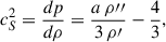
For each individual of the final population a value of complexity is computed. By representing the functional forms as trees, one can define in a natural way a measure of their complexities as the number of nodes in the tree. The combination of two variables by an operator (multiplication, addition, subtraction, division, power) has a complexity of three. The application of an operator to a variable or combination of variables (logarithm, exponential) has a complexity of two. Similarly, the combination of one variable and a constant by an operator (e.g. negation, inversion, square, cube, duplication) has a complexity of two. When counting the nodes in the example shown in Fig. 2 for the model A/[Da−ln(Da)], which we discuss in Sect. 5, shows this functional form has a complexity of ten. The complexity is used to compute a merit score to each elements of the final population.
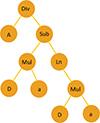 |
Fig. 2. Representation of the function A/[Da−ln(Da)] of complexity ten as a tree generated from the GP algorithm. |
4.2. Results
One run of CosmoGen produces a final population of o(102) models. We considered 512 models per generation throughout the search that added to the initial population size, which corresponds to a total of 8192 models involved in the full run. Each model was evaluated with the three-parameter Metropolis-Hastings MCMC. Due to the computational cost, we ran short chains and only one per model. We made preliminary tests of the step size and chain length and concluded that, in general, the chains started to stall when sampling around the posterior maximum, after less than 1000 points. This prompted us to set the chain length to 1200 points. With such a limit, not all tested models reached convergence, and some high fitness models may have been missed, biasing the sample towards lower fitness models. However, our goal is not be exhaustive but to find a small number of high fitness models to be further tested with better accuracy. With this setup, a typical run of the full process in 8 CPUs takes 240 hours.
The 20 best models are shown in Table 2. The functional form, score, minimum χ2, complexity, and best-fit parameters are indicated for each model. The models are ranked by score, where the ones with the lowest scores are considered best. This score parameter is the result of penalising the models according to their size and is definited by adding the model complexity to the fitness given by the minimum χ2 found in its MCMC. This metric is motivated by the Akaike information criteria (AIC; Akaike 1974), where models are penalised according to the number of free parameters by summing a χ2 to a linear function of the number of parameters. In our case, since all models have the same number of free parameters, the penalisable overparametrisation is not the number of parameters but the complexity of the dark energy expression. Since the complexity is of the same order of the delta χ2 between models, the unweighted sum we applied is a less severe penalty than the AIC expression. Examples of penalty factors are discussed in Rissanen (1978), which introduces a score with a stronger penalisation than AIC and the novel fitness function of Kartelj & Djukanovic (2023). The score is only used to rank the models at the end of the process and plays no role in the run.
Twenty best scoring models generated by the CosmoGen run.
We stress that the purpose of the short MCMC chains is to evaluate and select models. In other words, a high ranking shows that the model has a high likelihood for some combination of parameter values and is a strong candidate to be selected for the final population and additionally to become a parent. This conclusion can be made even with non-converged chains since the goal is not to estimate the posterior distribution. Therefore, this procedure does not guarantee that the model would remain among the top ranked ones after full MCMC analyses in a larger parameter space.
We selected one of the top ranked models for further investigation. In Sect. 5 we investigate its features and do a more complete MCMC analysis to verify if it indeed fulfils the goal of alleviating the tensions. For that analysis, we prefer a model with a good fitness score, low complexity, a reasonably looking functional form, and (if possible) resemblance with a known model. We selected the fifth ranked model from Table 2.
We also made several additional runs of CosmoGen to compare the resulting final populations and tested the robustness of the procedure. We present the discussion of those results in Appendix A.
5. Analysis of a selected model
We turn now to the analysis of the selected model defined by the following equation for the dark energy density,
 (8)
(8)
where the subscript CG stands for CosmoGen. This model closely resembles viable logarithmic scalar-field dark energy models discussed in the literature (see e.g. Wang et al. 2023).
In Fig. 3 we show the evolution of the CG energy density, normalised to the ΩΛ value of the Planck 2018 ΛCDM model today. Defining the model through its energy density allowed us to write the equation of state as function of the density and its derivatives through Eq. (1). Figure 4 shows the evolution of the equation of state of the CG fluid.
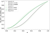 |
Fig. 3. Normalised energy density evolution for the CG dark energy fluid for different values of its free parameter D. |
 |
Fig. 4. Equation of state evolution for the CG dark energy fluid for different values of its free parameter D. |
The model clearly shows two distinct behaviours. For models with a positive log(D), the CG density increases earlier, and its equation of state crosses to the phantom regime and returns to less negative values. In contrast, models with a negative log(D) have a slow evolution of the equation of state.
Figures 5 and 6 show how the model predicted matter power spectrum and CMB temperature angular power spectrum depend on the free parameter D. Again there are two distinctive behaviours. Negative values of log(D) can get close to ΛCDM, while positive values show deviations up to 40% within the probed range.
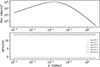 |
Fig. 5. Top panel: Matter power spectrum for the CG dark energy fluid for different values of D. Bottom panel: Deviation from ΛCDM. |
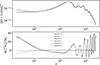 |
Fig. 6. Top panel: CMB temperature angular power spectrum for the CG dark energy fluid for different values of D. Bottom panel: Deviation from ΛCDM. |
We performed a likelihood analysis of the model to assess its viability and potential to alleviate cosmological tensions. For this, we no longer used the H0 and S8 priors that were used for model generation. Instead, we tested the model with structure formation data without imposing tension-related constraints. We made an analysis with CMB data (Planck 2018; Planck Collaboration VI 2020) and another with WL data (KiDS-Viking KV-450; Hildebrandt et al. 2020) We also performed an analysis of ΛCDM in the same conditions for comparison.
The parameter space consisted of the CG parameter D; the amplitude and slope of the primordial power spectrum, respectively As and ns; the baryon density, Ωb; the CDM density, ΩCDM; and the Hubble constant, h. The nuisance parameters we used are the APlanck for CMB and the amplitude of the intrinsic alignment model AIA for WL. We only considered flat models, and other cosmological and nuisance parameters were kept fixed. For all parameters, the analyses were done with flat priors. For D, we considered a log(D) range of [−5, 3]. The sampling was made with the PolyChord nested sampling method (Handley et al. 2015), with settings PCNlive = 150 (a large number of live points, to increase the accuracy of posteriors and evidence), PCNumRepeats = 30 (the number of slice-sampling steps to generate a new point, which is relevant for the reliability of the algorithm), and PCPrecisionCriterium = 0.001 (the end of sampling criterion; sampling terminates when the evidence contained in the live points is a 0.001 fraction of the total evidence).
The resulting constraints for the six basis and three derived parameters of the CG and ΛCDM models are shown in Table 3 (indicating the mean and 68% uncertainty estimated from each dataset) and in Figs. 7 and 8. The comparison between the CG model and the ΛCDM CMB contours in Fig. 7 (see also Table 3) shows that the CG model pushes H0 to higher values and Ωm to lower values. The constraints on these two parameters are broader for the CG model, but are comparable for most of the other parameters. The log(D) free parameter is constrained to be negative, as was already hinted at by the model behaviour shown in Figs. 3–6.
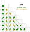 |
Fig. 7. CMB Planck 2018 analyses. Marginalised 2D 1σ and 2σ contours of the posterior and 1D marginalised posterior for the CG model (green) and ΛCDM (gold). |
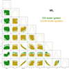 |
Fig. 8. WL KV-450 analyses. Marginalised 2D 1σ and 2σ contours of the posterior and 1D marginalised posterior for the CG model (green) and ΛCDM (gold). |
Mean and 68% uncertainty estimates for the CG and ΛCDM parameters from the two datasets.
The Bayes factor, also given in Table 3, indicates a weak preference for ΛCDM. We recall that a positive value of the logarithm of the Bayes factor, ℬ12, between models 1 and 2, has a larger strength of evidence for model 1 (Trotta 2008).
Regarding the WL analysis, the comparison between the CG model and the ΛCDM contours in Fig. 8 (see also Table 3) shows broad contours without significant differences between the two models.
To compare the behaviour of the two models for supernovae observables, we show in Fig. 9 the distance modulus computed for the CG and the ΛCDM models using the parameters obtained in Table 3 (for the CMB analysis). For reference, binned distance modulus measurements from the Joint Light-curve Analysis (JLA) sample (Betoule et al. 2014) are also plotted. The two curves are very close to each other, with the CG curve deviating from the ΛCDM one towards higher values on higher redshifts, supporting the findings of a larger Hubble constant.
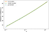 |
Fig. 9. Distance modulus as function of redshift for the GC (orange solid line) and ΛCDM (green dashed line) models using the Planck estimates of Table 3. The data points are from the JLA dataset. |
The H0 and S8 tensions are better seen in Figs. 10 and 11, which compare the relevant CMB and WL contours for each of the two models. The plots show a better agreement between the WL and the CMB contours in the case of the CG model. This is especially striking in contours that involve the S8 parameter.
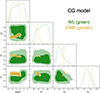 |
Fig. 10. CG model. Marginalised 2D 1σ and 2σ contours of the posterior and 1D marginalised posterior for the parameters relevant for the Hubble and S8 tensions for CMB Planck 2018 (gold) and WL KV-450 (green). |
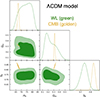 |
Fig. 11. ΛCDM model. Marginalised 2D 1σ and 2σ contours of the posterior and 1D marginalised posterior for the parameters relevant for the Hubble and S8 tensions for CMB Planck 2018 (gold) and WL KV-450 (green). |
We computed the tension, quantifying the discrepancy between the estimates of the parameter from two different datasets in the standard way in terms of the combined variances of the two estimates (e.g. Heymans et al. 2021). We find that the CG model shows a 1.1σS8 tension between the datasets, while for ΛCDM we found a larger value of 2.8σ. Concerning the Hubble tension, we did not quantify it, but we registered a 1σ shift of the Planck data H0 CG estimate with respect to the ΛCDM one towards higher values.
We thus conclude that this case study successfully contributes to the reduction of the tensions. This result is consistent with our approach of intentionally using a likelihood to that effect in the evaluation of the generated models.
6. Conclusions
We have presented a new type of cosmological tool, CosmoGen, that integrates traditional methods of numerical cosmology with ML techniques. We showed an example of how CosmoGen can provide new insights into cosmology. Incorporating evolutionary algorithms and likelihood sampling, the tool was applied to generate functional forms of ρDE(a) that reproduce key features of observational data. Notably, CosmoGen successfully identified fluid dark energy models capable of partially resolving the S8 and H0 tensions.
The potential of CosmoGen is far from fully explored. This tool has the capability to be expanded to generate other types of cosmological models, such as coupled species, unified dark matter, modified gravity theories as well as to map cosmological signatures.
The results we have presented were obtained using a standard laptop with 16 threads. This computational limitation restricted our ability to explore the full range of mathematical functions generated in a single run, leading to lists of candidate models that were often mathematically similar. For future development, optimising the code is crucial. The main limitation we encountered was that the stochastic GP method is not the most efficient evolutionary algorithm for sampling the space of possible equations. Further improvements of the code should incorporate alternative methods to improve the efficiency of the tool and expand its applicability. There are various other symbolic regression algorithms publicly available, most notably the exhaustive symbolic regression, developed for cosmological applications (Bartlett et al. 2024).
On the side of the cosmological likelihood sampling, there is also room for improvement. The option of relying on methods distributed with MontePython led us to use an MCMC method to find the best-fit parameters of the population models. Even though MCMC sampling is more robust in multi-peak distributions, it is very costly when compared to local minima finder optimisers. Indeed, the MCMC sampling spends precious time sampling a parameter space and provides much more information than what is strictly needed for model evaluation. In order to reduce computational cost, we imposed further limitations, such as (i) fixing most of the parameters in the evaluation step, (ii) considering dark energy functional forms with only one free parameter, and (iii) limiting the number of generations. These limitations will be addressed in the future development of CosmoGen.
Despite the current limitations in sampling resolution and algorithmic efficiency, the framework demonstrates the potential of integrating AI methods with the broadly used CLASS and MontePython cosmological tools. In this way, CosmoGen, opens a new window for cosmological model building.
Acknowledgments
We thank the anonymous referee for suggestions that led to an improvement of the paper. We also thank Antonio da Silva for useful discussions and acknowledge support from the Fundação para a Ciência e a Tecnologia (FCT) through R&D Unit funding UIDB/04434/2020 and UIDP/04434/2020.
References
- Abroshan, M., Mishra, S., & Khalili, M. M. 2023, Proceedings of the AAAI Conference on Artificial Intelligence [Google Scholar]
- Akaike, H. 1974, IEEE Trans. Autom. Control, 19, 716 [Google Scholar]
- Albrecht, A., Bernstein, G., Cahn, R., et al. 2006, ArXiv e-prints [arXiv:0609591] [Google Scholar]
- Arjona, R., & Nesseris, S. 2020, Phys. Rev. D, 101, 123525 [CrossRef] [Google Scholar]
- Audren, B., Lesgourgues, J., Benabed, K., & Prunet, S. 2013, JCAP, 2013, 001 [Google Scholar]
- Bartlett, D. J., Desmond, H., & Ferreira, P. G. 2024, IEEE Trans. Evol. Comput., 28, 950 [Google Scholar]
- Betoule, M., Kessler, R., Guy, J., et al. 2014, A&A, 568, A22 [NASA ADS] [CrossRef] [EDP Sciences] [Google Scholar]
- Blas, D., Lesgourgues, J., & Tram, T. 2011, JCAP, 2011, 034 [Google Scholar]
- Brinckmann, T., & Lesgourgues, J. 2019, Phys. Dark Universe, 26, 100378 [Google Scholar]
- Carbonell, J. G., Michalski, R. S., & Mitchell, T. M. 1983, in Machine Learning, eds. R. S. Michalski, J. G. Carbonell, & T. M. Mitchell (San Francisco, CA: Morgan Kaufmann), 3 [Google Scholar]
- Carleo, G., Cirac, I., Cranmer, K., et al. 2019, Rev. Mod. Phys., 91, 045002 [NASA ADS] [CrossRef] [Google Scholar]
- Delgado, A. M., Wadekar, D., Hadzhiyska, B., et al. 2022, MNRAS, 515, 2733 [NASA ADS] [CrossRef] [Google Scholar]
- DESI Collaboration (Abdul-Karim, M., et al.) 2025, Phys. Rev. D, 112, 083515 [Google Scholar]
- Di Valentino, E., Mena, O., Pan, S., et al. 2021, CQG, 38, 153001 [NASA ADS] [CrossRef] [Google Scholar]
- Euclid Collaboration (Mellier, Y., et al.) 2025, A&A, 697, A1 [Google Scholar]
- Fluke, C. J., & Jacobs, C. 2020, WIREs Data Min. Knowl. Discovery, 10, e1349 [Google Scholar]
- Goldberg, D. E. 1989, Genetic Algorithms in Search, Optimization and Machine Learning (Addison-Wesley) [Google Scholar]
- Handley, W. J., Hobson, M. P., & Lasenby, A. N. 2015, MNRAS, 450, L61 [NASA ADS] [CrossRef] [Google Scholar]
- Haupt, R., & Haupt, S. E. 2004, Practical Genetic Algorithms, 2nd edn. (Wyley) [Google Scholar]
- Heymans, C., Tröster, T., Asgari, M., et al. 2021, A&A, 646, A140 [NASA ADS] [CrossRef] [EDP Sciences] [Google Scholar]
- Hildebrandt, H., Viola, M., Heymans, C., et al. 2017, MNRAS, 465, 1454 [Google Scholar]
- Hildebrandt, H., Köhlinger, F., van den Busch, J. L., et al. 2020, A&A, 633, A69 [NASA ADS] [CrossRef] [EDP Sciences] [Google Scholar]
- Kartelj, A., & Djukanovic, M. 2023, J. Big Data, 10, 71 [Google Scholar]
- Koksbang, S. M. 2023, Phys. Rev. D, 107, 103522 [Google Scholar]
- Koza, J. R. 1992, Genetic Programming: On the Programming of Computers by Means of Natural Selection (Cambridge, MA: MIT Press) [Google Scholar]
- Kronberger, G., Borlacu, B., Kommenda, M., Winkler, S. M., & Affenzeller, M. 2024a, Symbolic Regression, 1st edn. (Boca Raton, FL: CRC Press / Taylor& Francis) [Google Scholar]
- Kronberger, G., Olivetti de Franca, F., Desmond, H., Bartlett, D. J., & Kammerer, L., 2024b, in Parallel Problem Solving from Nature– PPSN XVIII, eds. M. Affenzeller, S. M. Winkler, A. V. Kononova, et al. (Cham: Springer Nature Switzerland), 273 [Google Scholar]
- Lemos, P., Jeffrey, N., Cranmer, M., Ho, S., & Battaglia, P. 2023, Mach. Learn.: Sci. Technol., 4, 045002 [NASA ADS] [CrossRef] [Google Scholar]
- Lesgourgues, J. 2011, ArXiv e-prints [arXiv:1104.2932] [Google Scholar]
- Li, Y., Ni, Y., Croft, R. A. C., et al. 2021, Proc. Natl. Acad. Sci., 118, e2022038118 [Google Scholar]
- Linder, E. V. 2003, Phys. Rev. Lett., 90, 091301 [Google Scholar]
- LSST Science Collaboration (Abell, P. A., et al.) 2009, ArXiv e-prints [arXiv:0912.0201] [Google Scholar]
- Ntampaka, M., Avestruz, C., Boada, S., et al. 2019, BAAS, 51, 14 [Google Scholar]
- Perlmutter, S., Aldering, G., Goldhaber, G., et al. 1999, ApJ, 517, 565 [Google Scholar]
- Planck Collaboration VI. 2020, A&A, 641, A6 [NASA ADS] [CrossRef] [EDP Sciences] [Google Scholar]
- Planck Collaboration XVI. 2014, A&A, 571, A16 [NASA ADS] [CrossRef] [EDP Sciences] [Google Scholar]
- Riess, A. G., Filippenko, A. V., Challis, P., et al. 1998, AJ, 116, 1009 [Google Scholar]
- Riess, A. G., Macri, L. M., Hoffmann, S. L., et al. 2016, ApJ, 826, 56 [Google Scholar]
- Riess, A. G., Yuan, W., Macri, L. M., et al. 2022, ApJ, 934, L7 [NASA ADS] [CrossRef] [Google Scholar]
- Rissanen, J. 1978, Automatica, 14, 465 [CrossRef] [Google Scholar]
- Roman ROTAC and CCSDC. 2025, ArXiv e-prints [arXiv:2505.10574] [Google Scholar]
- Sutton, R., & Barto, A. 2018, in Reinforcement Learning, Second Edition: An Introduction (MIT Press), Adapt. Comput. Mach. Learn. Ser. [Google Scholar]
- Trotta, R. 2008, Contemp. Phys., 49, 71 [Google Scholar]
- Turing, A. M. 1950, Mind, LIX, 433 [CrossRef] [Google Scholar]
- Udrescu, S.-M., & Tegmark, M. 2020, Sci. Adv., 6, eaay2631 [Google Scholar]
- Vaswani, A., Shazeer, N., Parmar, N., et al. 2017, Advances in Neural Information Processing Systems (NeurIPS), 5998 [Google Scholar]
- Verde, L., Schöneberg, N., & Gil-Marín, H. 2024, ARA&A, 62, 287 [Google Scholar]
- Wadekar, D., Thiele, L., Hill, J. C., et al. 2023, MNRAS, 522, 2628 [NASA ADS] [CrossRef] [Google Scholar]
- Wang, D., Koussour, M., Malik, A., Myrzakulov, N., & Mustafa, G. 2023, Eur. Phys. J. C, 83, 670 [Google Scholar]
- Webb, S. A., & Goode, S. R. 2025, IAU Symp., 19, 40 [Google Scholar]
- Weinberg, S. 1989, Rev. Mod. Phys., 61, 1 [NASA ADS] [CrossRef] [Google Scholar]
- Wright, A. H., Stölzner, B., Asgari, M., et al. 2025, KiDS-Legacy: Cosmological Constraints From Cosmic Shear with the Complete Kilo-Degree Survey [Google Scholar]
- Zlatev, I., Wang, L., & Steinhardt, P. J. 1999, Phys. Rev. Lett., 82, 896 [Google Scholar]
Appendix A: Robustness tests
We show the top ranked models from two other runs of CosmoGen in Tables A.1 and A.2.
The 20 best scoring models generated by test run 1.
The 20 best scoring models generated by test run 2.
There are some models in common between the results of the various runs. We notice, however, that models from the same run seem to share some features, while the functional forms are more distinct between different runs. For example, in the case of Table A.1 there is a strong presence of logarithms, while in Table A.2 exponentials are more . This indicates that a larger initial population is required to accommodate a broad range of functions in a single run. Additionally, this highlights the lower efficiency of GP when compared to other symbolic regression methods, as discussed in Bartlett et al. (2024).
We also note that the χmin2 of these models are lower than those of Table 2. The main difference between the setups is that the evaluation MCMC chains used for Table 2 are shorter. It is also worth mentioning that, in contrast, the χmin2 values in Tables A.1 and A.2 are closer to the ΛCDM χmin2 for the same datasets.
It is also interesting to monitor the evolution through the generations. For this, we made new runs with longer chains, this time using the PolyChord nested sampling algorithm distributed in MontePython (Handley et al. 2015). An example run is shown in Table A.3. In there, we show the best models found in each of seven generations, and observe that the population globally evolves towards more complex and best-fit models.
The 5 best models of each generation in the Polychords run.
All Tables
Mean and 68% uncertainty estimates for the CG and ΛCDM parameters from the two datasets.
All Figures
|
Fig. 1. Flowchart showing the sequence of steps of a CosmoGen run. The ML component is enclosed in the solid red border, and the cosmological component is within the dashed blue border. The sequence of steps moves through the two components in a loop. The terms ‘GP’ and ‘MP’ stand for GP and MontePython, respectively. See text for a full description. |
| In the text | |
|
Fig. 2. Representation of the function A/[Da−ln(Da)] of complexity ten as a tree generated from the GP algorithm. |
| In the text | |
|
Fig. 3. Normalised energy density evolution for the CG dark energy fluid for different values of its free parameter D. |
| In the text | |
|
Fig. 4. Equation of state evolution for the CG dark energy fluid for different values of its free parameter D. |
| In the text | |
|
Fig. 5. Top panel: Matter power spectrum for the CG dark energy fluid for different values of D. Bottom panel: Deviation from ΛCDM. |
| In the text | |
|
Fig. 6. Top panel: CMB temperature angular power spectrum for the CG dark energy fluid for different values of D. Bottom panel: Deviation from ΛCDM. |
| In the text | |
|
Fig. 7. CMB Planck 2018 analyses. Marginalised 2D 1σ and 2σ contours of the posterior and 1D marginalised posterior for the CG model (green) and ΛCDM (gold). |
| In the text | |
|
Fig. 8. WL KV-450 analyses. Marginalised 2D 1σ and 2σ contours of the posterior and 1D marginalised posterior for the CG model (green) and ΛCDM (gold). |
| In the text | |
|
Fig. 9. Distance modulus as function of redshift for the GC (orange solid line) and ΛCDM (green dashed line) models using the Planck estimates of Table 3. The data points are from the JLA dataset. |
| In the text | |
|
Fig. 10. CG model. Marginalised 2D 1σ and 2σ contours of the posterior and 1D marginalised posterior for the parameters relevant for the Hubble and S8 tensions for CMB Planck 2018 (gold) and WL KV-450 (green). |
| In the text | |
|
Fig. 11. ΛCDM model. Marginalised 2D 1σ and 2σ contours of the posterior and 1D marginalised posterior for the parameters relevant for the Hubble and S8 tensions for CMB Planck 2018 (gold) and WL KV-450 (green). |
| In the text | |
Current usage metrics show cumulative count of Article Views (full-text article views including HTML views, PDF and ePub downloads, according to the available data) and Abstracts Views on Vision4Press platform.
Data correspond to usage on the plateform after 2015. The current usage metrics is available 48-96 hours after online publication and is updated daily on week days.
Initial download of the metrics may take a while.