| Issue |
A&A
Volume 693, January 2025
|
|
|---|---|---|
| Article Number | A58 | |
| Number of page(s) | 36 | |
| Section | Cosmology (including clusters of galaxies) | |
| DOI | https://doi.org/10.1051/0004-6361/202450859 | |
| Published online | 03 January 2025 | |
Euclid preparation
LIV. Sensitivity to neutrino parameters
1
Dipartimento di Fisica “Aldo Pontremoli”, Università degli Studi di Milano, Via Celoria 16, 20133 Milano, Italy
2
INFN-Sezione di Milano, Via Celoria 16, 20133 Milano, Italy
3
Institute for Theoretical Particle Physics and Cosmology (TTK), RWTH Aachen University, 52056 Aachen, Germany
4
Institut de Ciències del Cosmos (ICCUB), Universitat de Barcelona (IEEC-UB), Martí i Franquès 1, 08028 Barcelona, Spain
5
Institut für Theoretische Physik, University of Heidelberg, Philosophenweg 16, 69120 Heidelberg, Germany
6
Institut de Recherche en Astrophysique et Planétologie (IRAP), Université de Toulouse, CNRS, UPS, CNES, 14 Av. Edouard Belin, 31400 Toulouse, France
7
Université St Joseph; Faculty of Sciences, Beirut, Lebanon
8
Institute of Space Sciences (ICE, CSIC), Campus UAB, Carrer de Can Magrans, s/n, 08193 Barcelona, Spain
9
Dipartimento di Fisica, Università degli studi di Genova, and INFN-Sezione di Genova, via Dodecaneso 33, 16146 Genova, Italy
10
SISSA, International School for Advanced Studies, Via Bonomea 265, 34136 Trieste, TS, Italy
11
Department of Astrophysics, University of Zurich, Winterthurerstrasse 190, 8057 Zurich, Switzerland
12
AIM, CEA, CNRS, Université Paris-Saclay, Université de Paris, 91191 Gif-sur-Yvette, France
13
Dipartimento di Fisica, Università degli Studi di Torino, Via P. Giuria 1, 10125 Torino, Italy
14
INFN-Sezione di Torino, Via P. Giuria 1, 10125 Torino, Italy
15
INAF-Osservatorio Astrofisico di Torino, Via Osservatorio 20, 10025 Pino Torinese (TO), Italy
16
Hamburger Sternwarte, University of Hamburg, Gojenbergsweg 112, 21029 Hamburg, Germany
17
Dipartimento di Fisica - Sezione di Astronomia, Università di Trieste, Via Tiepolo 11, 34131 Trieste, Italy
18
INAF-Osservatorio Astronomico di Trieste, Via G. B. Tiepolo 11, 34143 Trieste, Italy
19
IFPU, Institute for Fundamental Physics of the Universe, via Beirut 2, 34151 Trieste, Italy
20
INAF-IASF Milano, Via Alfonso Corti 12, 20133 Milano, Italy
21
Université Libre de Bruxelles (ULB), Service de Physique Théorique CP225, Boulevard du Triophe, 1050 Bruxelles, Belgium
22
Department of Physics “E. Pancini”, University Federico II, Via Cinthia 6, 80126 Napoli, Italy
23
Ludwig-Maximilians-University, Schellingstrasse 4, 80799 Munich, Germany
24
INFN, Sezione di Trieste, Via Valerio 2, 34127 Trieste, TS, Italy
25
Department of Physics and Astronomy, University of British Columbia, Vancouver, BC V6T 1Z1, Canada
26
ICSC - Centro Nazionale di Ricerca in High Performance Computing, Big Data e Quantum Computing, Via Magnanelli 2, Bologna, Italy
27
School of Mathematics and Physics, University of Surrey, Guildford, Surrey GU2 7XH, UK
28
INAF-Osservatorio Astronomico di Brera, Via Brera 28, 20122 Milano, Italy
29
INAF-Osservatorio di Astrofisica e Scienza dello Spazio di Bologna, Via Piero Gobetti 93/3, 40129 Bologna, Italy
30
Dipartimento di Fisica e Astronomia, Università di Bologna, Via Gobetti 93/2, 40129 Bologna, Italy
31
INFN-Sezione di Bologna, Viale Berti Pichat 6/2, 40127 Bologna, Italy
32
Max Planck Institute for Extraterrestrial Physics, Giessenbachstr. 1, 85748 Garching, Germany
33
Dipartimento di Fisica, Università di Genova, Via Dodecaneso 33, 16146 Genova, Italy
34
INFN-Sezione di Genova, Via Dodecaneso 33, 16146 Genova, Italy
35
INAF-Osservatorio Astronomico di Capodimonte, Via Moiariello 16, 80131 Napoli, Italy
36
INFN section of Naples, Via Cinthia 6, 80126 Napoli, Italy
37
Instituto de Astrofísica e Ciências do Espaço, Universidade do Porto, CAUP, Rua das Estrelas, T4150-762 Porto, Portugal
38
INAF-Osservatorio Astronomico di Roma, Via Frascati 33, 00078 Monteporzio Catone, Italy
39
INFN-Sezione di Roma, Piazzale Aldo Moro, 2 - c/o Dipartimento di Fisica, Edificio G. Marconi, 00185 Roma, Italy
40
Institut de Física d’Altes Energies (IFAE), The Barcelona Institute of Science and Technology, Campus UAB, 08193 Bellaterra (Barcelona), Spain
41
Port d’Informació Científica, Campus UAB, C. Albareda s/n, 08193 Bellaterra (Barcelona), Spain
42
Dipartimento di Fisica e Astronomia “Augusto Righi” - Alma Mater Studiorum Università di Bologna, Viale Berti Pichat 6/2, 40127 Bologna, Italy
43
Institute for Astronomy, University of Edinburgh, Royal Observatory, Blackford Hill, Edinburgh EH9 3HJ, UK
44
Jodrell Bank Centre for Astrophysics, Department of Physics and Astronomy, University of Manchester, Oxford Road, Manchester M13 9PL, UK
45
European Space Agency/ESRIN, Largo Galileo Galilei 1, 00044 Frascati, Roma, Italy
46
ESAC/ESA, Camino Bajo del Castillo, s/n., Urb. Villafranca del Castillo, 28692 Villanueva de la Cañada, Madrid, Spain
47
Université Claude Bernard Lyon 1, CNRS/IN2P3, IP2I Lyon, UMR 5822, Villeurbanne F-69100, France
48
Institute of Physics, Laboratory of Astrophysics, Ecole Polytechnique Fédérale de Lausanne (EPFL), Observatoire de Sauverny, 1290 Versoix, Switzerland
49
UCB Lyon 1, CNRS/IN2P3, IUF, IP2I Lyon, 4 rue Enrico Fermi, 69622 Villeurbanne, France
50
Departamento de Física, Faculdade de Ciências, Universidade de Lisboa, Edifício C8, Campo Grande, PT1749-016 Lisboa, Portugal
51
Instituto de Astrofísica e Ciências do Espaço, Faculdade de Ciências, Universidade de Lisboa, Campo Grande, 1749-016 Lisboa, Portugal
52
Department of Astronomy, University of Geneva, ch. d’Ecogia 16, 1290 Versoix, Switzerland
53
Université Paris-Saclay, CNRS, Institut d’astrophysique spatiale, 91405 Orsay, France
54
Department of Physics, Oxford University, Keble Road, Oxford OX1 3RH, UK
55
INFN-Padova, Via Marzolo 8, 35131 Padova, Italy
56
INAF-Istituto di Astrofisica e Planetologia Spaziali, via del Fosso del Cavaliere, 100, 00100 Roma, Italy
57
Université Paris-Saclay, Université Paris Cité, CEA, CNRS, AIM, 91191 Gif-sur-Yvette, France
58
Istituto Nazionale di Fisica Nucleare, Sezione di Bologna, Via Irnerio 46, 40126 Bologna, Italy
59
INAF-Osservatorio Astronomico di Padova, Via dell’Osservatorio 5, 35122 Padova, Italy
60
Universitäts-Sternwarte München, Fakultät für Physik, Ludwig-Maximilians-Universität München, Scheinerstrasse 1, 81679 München, Germany
61
Institute of Theoretical Astrophysics, University of Oslo, P.O. Box 1029 Blindern, 0315 Oslo, Norway
62
Leiden Observatory, Leiden University, Einsteinweg 55, 2333 CC Leiden, The Netherlands
63
von Hoerner & Sulger GmbH, Schlossplatz 8, 68723 Schwetzingen, Germany
64
Technical University of Denmark, Elektrovej 327, 2800 Kgs. Lyngby, Denmark
65
Cosmic Dawn Center (DAWN), Copenhagen, Denmark
66
Max-Planck-Institut für Astronomie, Königstuhl 17, 69117 Heidelberg, Germany
67
Department of Physics and Astronomy, University College London, Gower Street, London WC1E 6BT, UK
68
Department of Physics and Helsinki Institute of Physics, Gustaf Hällströmin katu 2, 00014 University of Helsinki, Helsinki, Finland
69
Aix-Marseille Université, CNRS/IN2P3, CPPM, Marseille, France
70
Jet Propulsion Laboratory, California Institute of Technology, 4800 Oak Grove Drive, Pasadena, CA 91109, USA
71
Mullard Space Science Laboratory, University College London, Holmbury St Mary, Dorking, Surrey RH5 6NT, UK
72
Université de Genève, Département de Physique Théorique and Centre for Astroparticle Physics, 24 quai Ernest-Ansermet, CH-1211 Genève 4, Switzerland
73
Department of Physics, P.O. Box 64 00014 University of Helsinki, Helsinki, Finland
74
Helsinki Institute of Physics, Gustaf Hällströmin katu 2, University of Helsinki, Helsinki, Finland
75
NOVA optical infrared instrumentation group at ASTRON, Oude Hoogeveensedijk 4, 7991PD Dwingeloo, The Netherlands
76
Universität Bonn, Argelander-Institut für Astronomie, Auf dem Hügel 71, 53121 Bonn, Germany
77
Aix-Marseille Université, CNRS, CNES, LAM, Marseille, France
78
Dipartimento di Fisica e Astronomia “Augusto Righi” - Alma Mater Studiorum Università di Bologna, via Piero Gobetti 93/2, 40129 Bologna, Italy
79
Department of Physics, Institute for Computational Cosmology, Durham University, South Road, DH1 3LE Durham, UK
80
Université Côte d’Azur, Observatoire de la Côte d’Azur, CNRS, Laboratoire Lagrange, Bd de l’Observatoire, CS 34229, 06304 Nice cedex 4, France
81
Institut d’Astrophysique de Paris, UMR 7095, CNRS, and Sorbonne Université, 98 bis boulevard Arago, 75014 Paris, France
82
Université Paris Cité, CNRS, Astroparticule et Cosmologie, 75013 Paris, France
83
Institut d’Astrophysique de Paris, 98bis Boulevard Arago, 75014 Paris, France
84
European Space Agency/ESTEC, Keplerlaan 1, 2201 AZ Noordwijk, The Netherlands
85
School of Mathematics, Statistics and Physics, Newcastle University, Herschel Building, Newcastle-upon-Tyne NE1 7RU, UK
86
Department of Physics and Astronomy, University of Aarhus, Ny Munkegade 120, DK-8000 Aarhus C, Denmark
87
Waterloo Centre for Astrophysics, University of Waterloo, Waterloo, Ontario N2L 3G1, Canada
88
Department of Physics and Astronomy, University of Waterloo, Waterloo, Ontario N2L 3G1, Canada
89
Perimeter Institute for Theoretical Physics, Waterloo, Ontario N2L 2Y5, Canada
90
Université Paris-Saclay, Université Paris Cité, CEA, CNRS, Astrophysique, Instrumentation et Modélisation Paris-Saclay, 91191 Gif-sur-Yvette, France
91
Space Science Data Center, Italian Space Agency, via del Politecnico snc, 00133 Roma, Italy
92
Centre National d’Etudes Spatiales – Centre spatial de Toulouse, 18 avenue Edouard Belin, 31401 Toulouse Cedex 9, France
93
Institute of Space Science, Str. Atomistilor, nr. 409 Măgurele, Ilfov 077125, Romania
94
Instituto de Astrofísica de Canarias, Calle Vía Láctea s/n, 38204 San Cristóbal de La Laguna, Tenerife, Spain
95
Departamento de Astrofísica, Universidad de La Laguna, 38206 La Laguna, Tenerife, Spain
96
Dipartimento di Fisica e Astronomia “G. Galilei”, Università di Padova, Via Marzolo 8, 35131 Padova, Italy
97
Departamento de Física, FCFM, Universidad de Chile, Blanco Encalada 2008, Santiago, Chile
98
Universität Innsbruck, Institut für Astro- und Teilchenphysik, Technikerstr. 25/8, 6020 Innsbruck, Austria
99
Institut d’Estudis Espacials de Catalunya (IEEC), Edifici RDIT, Campus UPC, 08860 Castelldefels, Barcelona, Spain
100
Satlantis, University Science Park, Sede Bld 48940, Leioa-Bilbao, Spain
101
Centro de Investigaciones Energéticas, Medioambientales y Tecnológicas (CIEMAT), Avenida Complutense 40, 28040 Madrid, Spain
102
Instituto de Astrofísica e Ciências do Espaço, Faculdade de Ciências, Universidade de Lisboa, Tapada da Ajuda, 1349-018 Lisboa, Portugal
103
Universidad Politécnica de Cartagena, Departamento de Electrónica y Tecnología de Computadoras, Plaza del Hospital 1, 30202 Cartagena, Spain
104
INFN-Bologna, Via Irnerio 46, 40126 Bologna, Italy
105
Infrared Processing and Analysis Center, California Institute of Technology, Pasadena, CA 91125, USA
106
INAF, Istituto di Radioastronomia, Via Piero Gobetti 101, 40129 Bologna, Italy
107
Astronomical Observatory of the Autonomous Region of the Aosta Valley (OAVdA), Loc. Lignan 39, I-11020 Nus (Aosta Valley), Italy
108
Institut de Ciencies de l’Espai (IEEC-CSIC), Campus UAB, Carrer de Can Magrans, s/n Cerdanyola del Vallés, 08193 Barcelona, Spain
109
Center for Computational Astrophysics, Flatiron Institute, 162 5th Avenue, 10010 New York, NY, USA
110
School of Physics and Astronomy, Cardiff University, The Parade, Cardiff CF24 3AA, UK
111
Centre de Calcul de l’IN2P3/CNRS, 21 avenue Pierre de Coubertin, 69627 Villeurbanne Cedex, France
112
Junia, EPA department, 41 Bd Vauban, 59800 Lille, France
113
Instituto de Física Teórica UAM-CSIC, Campus de Cantoblanco, 28049 Madrid, Spain
114
CERCA/ISO, Department of Physics, Case Western Reserve University, 10900 Euclid Avenue, Cleveland, OH 44106, USA
115
Laboratoire Univers et Théorie, Observatoire de Paris, Université PSL, Université Paris Cité, CNRS, 92190 Meudon, France
116
Dipartimento di Fisica e Scienze della Terra, Università degli Studi di Ferrara, Via Giuseppe Saragat 1, 44122 Ferrara, Italy
117
Istituto Nazionale di Fisica Nucleare, Sezione di Ferrara, Via Giuseppe Saragat 1, 44122 Ferrara, Italy
118
Institut de Physique Théorique, CEA, CNRS, Université Paris-Saclay, 91191 Gif-sur-Yvette Cedex, France
119
Minnesota Institute for Astrophysics, University of Minnesota, 116 Church St SE, Minneapolis, MN 55455, USA
120
Institute Lorentz, Leiden University, Niels Bohrweg 2, 2333 CA Leiden, The Netherlands
121
Institute for Astronomy, University of Hawaii, 2680 Woodlawn Drive, Honolulu, HI 96822, USA
122
Department of Physics & Astronomy, University of California Irvine, Irvine CA 92697, USA
123
Department of Astronomy & Physics and Institute for Computational Astrophysics, Saint Mary’s University, 923 Robie Street, Halifax, Nova Scotia B3H 3C3, Canada
124
Departamento Física Aplicada, Universidad Politécnica de Cartagena, Campus Muralla del Mar, 30202 Cartagena, Murcia, Spain
125
Institute of Cosmology and Gravitation, University of Portsmouth, Portsmouth PO1 3FX, UK
126
Department of Computer Science, Aalto University, PO Box 15400 Espoo FI-00 076, Finland
127
Ruhr University Bochum, Faculty of Physics and Astronomy, Astronomical Institute (AIRUB), German Centre for Cosmological Lensing (GCCL), 44780 Bochum, Germany
128
Université Paris-Saclay, CNRS/IN2P3, IJCLab, 91405 Orsay, France
129
Department of Physics and Astronomy, Vesilinnantie 5, 20014 University of Turku, Finland
130
Serco for European Space Agency (ESA), Camino bajo del Castillo, s/n, Urbanizacion Villafranca del Castillo, Villanueva de la Cañada, 28692 Madrid, Spain
131
ARC Centre of Excellence for Dark Matter Particle Physics, Melbourne, Australia
132
Centre for Astrophysics & Supercomputing, Swinburne University of Technology, Victoria 3122, Australia
133
W.M. Keck Observatory, 65-1120 Mamalahoa Hwy, Kamuela, HI, USA
134
School of Physics and Astronomy, Queen Mary University of London, Mile End Road, London E1 4NS, UK
135
Department of Physics and Astronomy, University of the Western Cape, Bellville, Cape Town 7535, South Africa
136
ICTP South American Institute for Fundamental Research, Instituto de Física Teórica, Universidade Estadual Paulista, São Paulo, Brazil
137
Oskar Klein Centre for Cosmoparticle Physics, Department of Physics, Stockholm University, Stockholm SE-106 91, Sweden
138
Astrophysics Group, Blackett Laboratory, Imperial College London, London SW7 2AZ, UK
139
Univ. Grenoble Alpes, CNRS, Grenoble INP, LPSC-IN2P3, 53, Avenue des Martyrs, 38000 Grenoble, France
140
INAF-Osservatorio Astrofisico di Arcetri, Largo E. Fermi 5, 50125 Firenze, Italy
141
Dipartimento di Fisica, Sapienza Università di Roma, Piazzale Aldo Moro 2, 00185 Roma, Italy
142
Centro de Astrofísica da Universidade do Porto, Rua das Estrelas, 4150-762 Porto, Portugal
143
Dipartimento di Fisica, Università di Roma Tor Vergata, Via della Ricerca Scientifica 1, Roma, Italy
144
INFN, Sezione di Roma 2, Via della Ricerca Scientifica 1, Roma, Italy
145
Institute of Astronomy, University of Cambridge, Madingley Road Cambridge CB3 0HA, UK
146
Theoretical astrophysics, Department of Physics and Astronomy, Uppsala University, Box 515 751 20 Uppsala, Sweden
147
Department of Astrophysical Sciences, Peyton Hall, Princeton University, Princeton, NJ 08544, USA
148
Niels Bohr Institute, University of Copenhagen, Jagtvej 128, 2200 Copenhagen, Denmark
149
Center for Cosmology and Particle Physics, Department of Physics, New York University, New York, NY 10003, USA
⋆ Corresponding author; maria.archidiacono@unimi.it
Received:
24
May
2024
Accepted:
6
October
2024
Context. The Euclid mission of the European Space Agency will deliver weak gravitational lensing and galaxy clustering surveys that can be used to constrain the standard cosmological model and extensions thereof.
Aims. We present forecasts from the combination of the Euclid photometric galaxy surveys (weak lensing, galaxy clustering, and their cross-correlations) and its spectroscopic redshift survey with respect to their sensitivity to cosmological parameters. We include the summed neutrino mass, ∑mν, and the effective number of relativistic species, Neff, in the standard ΛCDM scenario and in the dynamical dark energy (w0waCDM) scenario.
Methods. We compared the accuracy of different algorithms predicting the non-linear matter power spectrum for such models. We then validated several pipelines for Fisher matrix and Markov chain Monte Carlo (MCMC) forecasts, using different theory codes, algorithms for numerical derivatives, and assumptions on the non-linear cut-off scale.
Results. The Euclid primary probes alone will reach a sensitivity of σ(∑mν = 60 meV) = 56 meV in the ΛCDM+∑mν model, whereas the combination with cosmic microwave background (CMB) data from Planck is expected to achieve σ(∑mν) = 23 meV, offering evidence of a non-zero neutrino mass to at least the 2.6 σ level. This could be pushed to a 4 σ detection if future CMB data from LiteBIRD and CMB Stage-IV were included. In combination with Planck, Euclid will also deliver tight constraints on ΔNeff < 0.144 (95%CL) in the ΛCDM+∑mν+Neff model or even ΔNeff < 0.063 when future CMB data are included. When floating the dark energy parameters, we find that the sensitivity to Neff remains stable, but for ∑mν, it gets degraded by up to a factor of 2, at most.
Conclusions. This work illustrates the complementarity among the Euclid spectroscopic and photometric surveys and among Euclid and CMB constraints. Euclid will offer great potential in measuring the neutrino mass and excluding well-motivated scenarios with additional relativistic particles.
Key words: large-scale structure of Universe
© The Authors 2024
 Open Access article, published by EDP Sciences, under the terms of the Creative Commons Attribution License (https://creativecommons.org/licenses/by/4.0), which permits unrestricted use, distribution, and reproduction in any medium, provided the original work is properly cited.
This article is published in open access under the Subscribe to Open model. Subscribe to A&A to support open access publication.
1. Introduction
Over the last two decades, the continuous improvement of the precision and accuracy of cosmological observations has opened a window to constraining neutrino properties via cosmological data. In particular, the sum of the three neutrino masses can be well constrained due to its effect of suppressing the clustering of cold dark matter after the neutrino non-relativistic transition.
Neutrino oscillation experiments demonstrated that at least two neutrinos are massive by measuring two squared mass differences Δmij2 = mi2 − mj2 as
where the sign of Δm3i2 depends on the mass ordering, which can be either normal (NO: m1 < m2 < m3, Δm3i2 = Δm312 > 0) or inverted (IO: m3 < m1 < m2, Δm3i2 = Δm322 < 0), see Esteban et al. (2020), Gonzalez-Garcia & Yokoyama (2022). According to these results, the minimum value of the neutrino mass sum is either 0.06 eV1 in NO or 0.10 eV in IO. However, neutrino oscillation experiments cannot constrain the absolute neutrino mass sum. On the other hand, β-decay experiments are sensitive to the effective electron anti-neutrino mass. Recently, the Karlsruhe Tritium Neutrino Experiment (KATRIN) constrained mν < 0.45 eV (90% CL, see Aker et al. 2024). Future β-decay experiments, such as Project 8 (Project 8 Collaboration 2022), could potentially reach a sensitivity of 40 meV.
Despite the great progress made in the precision of β-decay experiments2, cosmology provides the most stringent (albeit model-dependent) constraints to date on the absolute neutrino mass scale. The Planck Collaboration reported an upper bound of ∑mν < 0.24 eV (95% CL) by combining the temperature,
polarisation, and lensing of the cosmic microwave background (CMB). Adding external baryon acoustic oscillation (BAO) data further improves the bound to ∑mν < 0.12 eV (95% CL, see Planck Collaboration VI 2020). Including Pantheon type Ia supernovae, baryon acoustic oscillations and redshift-space distortions from the Sloan Digital Sky Survey and weak-lensing measurements from the Dark Energy Survey leads to an upper bound of 0.11 eV (Alam et al. 2021). Recently, the DESI Collaboration reported an upper limit of ∑mν < 0.072 eV at the 95% CL from the combination of DESI BAO and CMB data. This bound mildly favours the NO scenario and shows that there might be a possibility of indirectly constraining the neutrino mass hierarchy using cosmological data. Current data on the full-shape galaxy power spectrum do not yet improve the constraint on ∑mν compared to the combination of CMB and the BAO geometric information (Ivanov et al. 2020a), but future galaxy surveys are expected to improve it. Finally, it is important to reiterate that changing the underlying cosmological model could potentially relax the constraints obtained from many of the cosmological probes (Lambiase et al. 2019; di Valentino et al. 2022).
The ability of cosmology to constrain the neutrino mass paved the way to investigate, via cosmological data, additional neutrino properties and particularly the number density of neutrinos. The standard model of particles physics predicts three active neutrino species, as confirmed by accelerator experiments (Mele 2015). In cosmology, this would correspond to an effective neutrino number Neff = 3 in the instantaneous decoupling limit, or (when sticking to the same definition of this effective number) to Neff = 3.044 when neutrino decoupling is modelled accurately (Froustey et al. 2020; Akita & Yamaguchi 2020; Bennett et al. 2021). Any deviation from this value is a hint at non-standard physics in the neutrino sector (e.g. low-temperature reheating, non-thermal corrections to the neutrino distribution generated by new physics, non-standard neutrino interactions or sterile neutrinos, Dvorkin et al. 2022; Archidiacono & Gariazzo 2022; Dasgupta & Kopp 2021), or exotic radiation components (e.g. axions or other forms of dark radiation, Marsh 2016; Kawasaki & Nakayama 2013; Di Luzio et al. 2020).
The continuous improvement of cosmological constraints on neutrino properties has opened up the question of whether upcoming cosmological surveys will be able to deliver a detection of a non-zero neutrino mass, to distinguish between the IO and NO scenarios due to a tight upper limit, and to investigate additional neutrino properties. One of the primary science goals of Euclid is to improve the cosmological constraints on the neutrino mass, possibly delivering evidence for a non-zero value. The aim of this work is to assess the sensitivity of Euclid to the neutrino mass, as well as its robustness against variations of the number of neutrinos or the modelling of dark energy.
Euclid (Euclid Collaboration 2024d) is a medium-class mission of the European Space Agency, which will map the Local Universe to improve our understanding of the expansion history and of the growth of structures. The satellite will observe roughly 14 000 deg2 of the sky through two instruments, a visible imager (VIS, Euclid Collaboration 2024b) and Near-Infrared Spectrometer and Photometer (NISP, Euclid Collaboration 2024c), delivering the images of more than one billion galaxies and the spectra of between 20 and 30 million galaxies out to a redshift of about 2. The combination of spectroscopy and photometry will allow us to measure galaxy clustering and weak gravitational lensing, aiming at a 1% level of accuracy in the corresponding power spectra.
The paper is organised as follows. In Sect. 2, we review the main effects of massive neutrinos in cosmology and discuss their impact on the theoretical predictions for Euclid observables in Sect. 3. In Sect. 4 we introduce additional probes like cluster number counts from Euclid itself and external CMB data, which are potentially very synergistic with Euclid primary (weak lensing and galaxy clustering) probes. The methodology used to perform the forecast is described in Sect. 5, the code is validated in Sect. 6, and the results are presented in Sect. 7. Finally, we draw our conclusions on the sensitivity of Euclid to neutrino physics in Sect. 8. Along the main text, we point the reader to several Appendices A, B, C, D, E, F, G, and H, providing technical details on the analysis, as well as additional figures and consistency checks.
2. Neutrino cosmology
In the following, we briefly review the main effects of the neutrino masses and number density on structure formation. For a thorough description, we refer the readers to Bashinsky & Seljak (2004), Hannestad (2006), Lesgourgues & Pastor (2006, 2012), Lesgourgues et al. (2013), Lattanzi & Gerbino (2018), Archidiacono et al. (2017, 2020), and Lesgourgues & Verde (2022).
2.1. Massive neutrinos
Massive neutrinos play an important role in the distribution of large-scale structures. They decouple from the primordial plasma around T ∼ 1 MeV, while still being relativistic. The redshift znr at which they enter the non-relativistic regime depends on the individual mass, mν, of each neutrino as (1 + znr)∼2 × 10³(mν/1 eV). After decoupling, neutrinos travel with a thermal velocity, vth, that defines the neutrino free-streaming wavenumber (Lesgourgues & Pastor 2006) as
where  is the total background density, a is the scale factor, and GontN is the Newton constant. After the non-relativistic transition the thermal velocity decays as vth = ⟨p⟩ mν−1 ∝ a−1, therefore, the free-streaming wavenumber goes through a minimum value of
  at the time of the non-relativistic transition; here h = H0/(100 km s−1 Mpc−1) is the reduced Hubble parameter. Neutrinos cannot cluster in regions smaller than their free-streaming length (λFS = 2πa/kFS). On scales larger than the maximum free-streaming length, corresponding to k < knr, massive neutrinos always behave as cold dark matter and the power spectrum of matter density fluctuations, Pmm(k), does not change with respect to the power spectrum of a cosmology that assumes the neutrinos are massless, but their non-relativistic density is added to that of cold dark matter. On the other hand, on scales smaller than the current value of the free-streaming length (k > kFS0), massive neutrinos induce a suppression of the linear matter spectrum, Pmm(k), at a redshift of z = 0 by approximately, ΔPmm(k)/Pmm(k)≃ − 8fν, where fν = Ων, 0/Ωm, 0 is the fraction of neutrino with respect to matter density (Hu et al. 1998; Lesgourgues et al. 2013). The reason is twofold: on scales where neutrinos are free-streaming, they do not contribute to gravitational clustering; and they slow down the growth of cold dark matter perturbations, which is given by a1 − 3fν/5 during matter domination (Bond et al. 1980). The second effect is responsible for the majority of the overall suppression and the scale dependence of the linear growth factor induced by massive neutrinos must be taken into account in the modelling of large-scale structure observables (see Sect. 3).
An important consideration is that the suppression of the power spectrum (as well as the effect of neutrino masses on the CMB spectrum) is almost the same independently of which neutrino ordering (IO or NO) is present in nature. This has been shown, for example, in Lesgourgues et al. (2004), Lesgourgues & Pastor (2006) and Archidiacono et al. (2020). Indeed, the cosmological observables are mainly sensitive to fν, that is, to Ων, 0 h2 ≈ ∑mν/(93.12 eV), and thus, to the summed neutrino mass, ∑mν (see Mangano et al. 2005)3.
The step-like suppression induced by neutrino free streaming is best seen when varying ∑mν while fixing the density of total matter, the density of baryonic matter, and the fractional density of the cosmological constant, namely, the parameters {Ωm, 0h2, Ωb, 0h2, ΩΛ}. This is illustrated in the top panel of Fig. 1. However, such a transformation also changes characteristic times and scales that are strongly constrained by CMB experiments, such as the redshift of equality between radiation and matter or the angular diameter distance to the last-scattering surface. To understand what is left for such experiments as Euclid to measure, given our knowledge of the CMB spectrum, it makes more sense to look at the variation in the matter power spectrum when floating ∑mν, while fixing the redshift of equality, baryonic matter density, and angular scale of the sound horizon at decoupling (Archidiacono et al. 2017; Lesgourgues & Verde 2022). In particular, this means fixing the parameters {Ωc, 0h2, Ωb, 0h2, θs}, where Ωc, 0 accounts for the fractional density of cold dark matter only. We note that neutrinos with a realistic mass were still relativistic at the time of radiation-to-matter equality, so that for a fixed CMB temperature and effective neutrino number, the redshift of equality is fixed by (Ωc, 0 + Ωb, 0)h2 – and not by Ωm, 0h2 = (Ωb, 0 + Ωc, 0 + Ων, 0)h2. In that case, the effect of the neutrino mass is displayed in the bottom panel of Fig. 1. The increase in ∑mν with a fixed θs implies a decrease of h that suppresses the large-scale power spectrum roughly by the same amount as neutrino free-streaming suppresses the small-scale power spectrum. As a result, in a combined fit to Euclid data and CMB data from (for instance) Planck, the neutrino mass would manifest itself mainly as an overall decrease of the amplitude of the matter power spectrum relative to that measured at the time of decoupling by CMB data. This decrease is slightly redshift dependent: the smaller the redshift, the more the power spectrum gets suppressed. Besides that, variations in ∑mν induce a small shift in BAO scales, responsible for the oscillations shown in the bottom panel of Fig. 1.
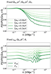 |
Fig. 1. Effects of the neutrino mass on the linear total matter (solid) or cold-plus-baryonic matter (dashed) power spectrum, presented as ratios with respect to the ΛCDM spectrum with massless neutrinos for four different values of the summed neutrino mass. Top: Singling out the effect of neutrino free-streaming, we keep the parameters {Ωm, 0h2, Ωb, 0h2, ΩΛ} fixed. Bottom: Quantities best constrained by CMB data, that is, {zeq, Ωb, 0h2, θs}, are fixed to show what is left for Euclid to measure. The mass is always equally split between the three neutrino species. |
The Euclid weak-lensing probe traces total matter, whereas (to a very good approximation) the galaxy clustering probe traces only the fluctuations of cold and baryonic dark matter (Castorina et al. 2014). The two panels in Fig. 1 also show the impact of varying ∑mν on the cold-plus-baryonic matter power spectrum, Pcc (dashed line). The effect of the neutrino mass on the amplitude of the linear small-scale spectrum, Pcc, is slightly reduced compared to the total matter case, with a suppression given roughly by ΔPcc(k)/Pcc(k)≃ − 6fν.
2.2. Number of relativistic species
The contribution of ultra-relativistic species to the background density of radiation, ρr (including that of neutrinos before their non-relativistic transition) can be parameterised in terms of an effective number of neutrinos Neff as
![$$ \begin{aligned} \rho _{\rm r} = \left[1 + \frac{7}{8}\left(\frac{4}{11}\right)^{4/3}N_{\rm eff}\right]\rho _{\gamma }, \end{aligned} $$](/articles/aa/full_html/2025/01/aa50859-24/aa50859-24-eq5.gif)
where ργ stands for the photon background density. In the above expression, the factor 7/8 accounts for the Fermi–Dirac statistics of neutrinos, and (4/11)4/3 accounts for the neutrino-to-photon temperature ratio in the instantaneous decoupling approximation (Lesgourgues & Pastor 2006). We would expect Neff = 3 for three standard model neutrinos that thermalised in the early Universe and decoupled well before electron-positron annihilation. However, theoretical predictions set Neff = 3.044 in the standard cosmological model (Mangano et al. 2002; Froustey et al. 2020; Bennett et al. 2021; Drewes et al. 2024) because neutrinos decouple gradually with residual scatterings during this time4. This value would change in the presence of non-standard neutrino features (see for example Lesgourgues et al. 2013, for the case of a large leptonic asymmetry, non-thermal distortions from low-temperature reheating, non-standard interactions, etc.), or additional relativistic relics contributing to the energy budget (see for example Dvorkin et al. 2022).
At the level of background cosmology all these effects and models are captured by a single parameter Neff. However, at the level of perturbations some model-dependent features may arise, for instance if the additional relics carry small masses or feature (self-)interactions. In this work, for simplicity, we stick to the class of models where additional non-relativistic relics are decoupled, massless and free-streaming. However, we must simultaneously take the effect of neutrino masses into account – in most of our forecasts, {∑mν, Neff} are two free model parameters. In this work, we will consider two ways to distribute the total mass ∑mν over the different species.
-
(a)
By default, we considered three active neutrino species degenerate in mass (mν = ∑mν/3), thermally distributed and with a temperature chosen in such a way that each species contributes to Neff by 3.044/3. Then, the additional free-streaming and massless dark radiation mentioned before enhances the total effective neutrino number as Neff = 3.044 + ΔNeff with ΔNeff ≥ 0. In particular, this assumption is used throughout the results presented in Sect. 7. Considering three degenerate massive neutrinos offers the advantage of predicting a matter power spectrum nearly indistinguishable from that of the realistic NO and IO scenarios with the same total mass, while models with only one or two massive species provide poorer approximations (Lesgourgues et al. 2004; Lesgourgues & Pastor 2006; Archidiacono et al. 2020).
-
(b)
For the specific validation presented in Sect. 6, we adopted the same model as in most previous forecasts, both for the sake of comparison with earlier work and because the calculation of Fisher matrices is easier when parameters can vary symmetrically around their fiducial value. Then, like in the baseline analysis of Planck Collaboration VI (2020), we stuck to a single massive neutrino (mν = ∑mν), with the same thermal distribution and temperature as in the previous model. We considered additional free-streaming and massless species, contributing to the effective neutrino number by Neff − 3.044/3, such that Neff can be either bigger or smaller than 3.044.
We note that some of the models mentioned before (that feature non-standard physics in the neutrino sector) would require other model-dependent schemes for the splitting of the total mass across species and for the phase-space distribution of each massive species. However, the sensitivity of Euclid to the parameters ∑mν and Neff is expected to depend only weakly on each particular scheme, such that our sensitivity forecast assuming case (a) is representative of other cases.
The effect of varying Neff on the linear matter power spectrum depends on which other parameters are kept fixed. For instance, the top panel of Fig. 2 shows the impact of increasing Neff with fixed Ωm, 0, Ωb, 0, and h. The leading effect is then a shift in the redshift of equality, inducing a suppression of the power spectrum. However, like for neutrino masses, in order to understand what is left for Euclid to measure, it is interesting to fix the cosmological parameters that are best constrained by CMB data, namely the redshift of radiation-to-matter equality zeq, the baryon matter density, and the sound horizon angular scale (Hou et al. 2013; Lesgourgues et al. 2013; Lesgourgues & Verde 2022). With such a choice, the effect of varying Neff is displayed in the bottom panel of Fig. 2. Since zeq is given by the matter-to-radiation density ratio Ωm, 0/Ωr, 0, increasing the radiation density with a fixed baryon matter density implies an increase in the cold dark matter density, and thus, a decrease of the baryon-to-cold matter density ratio Ωb, 0/Ωc, 0. This has two well-known consequences: an enhancement of the amplitude of the matter power spectrum on scales k > keq, where  is the wavenumber crossing the Hubble radius at equality; and a decrease in the amplitude of BAO oscillations. The scale of BAO peaks is also slightly shifted due to an enhanced neutrino drag effect (Bashinsky & Seljak 2004; Lesgourgues et al. 2013; Baumann et al. 2019). In the bottom panel of Fig. 2, one can clearly identify the power enhancement at k > keq, as well as the oscillations produced by the shift in BAO phase and amplitude. The small power suppression on large scales comes from the fact that the matter fractional density, Ωm, 0, which controls the overall amplitude of the matter power spectrum on those scales, decreases slightly when we increase Ωm, 0h2, while fixing θs.
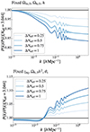 |
Fig. 2. Effect of the effective number of relativistic degrees of freedom Neff = 3.044 + ΔNeff on the linear total matter power spectrum, presented as ratios with respect to the ΛCDM spectrum with Neff = 3.044. Top: Density and Hubble parameters {Ωm, 0, Ωb, 0, h} fixed only. Bottom: Quantities best constrained by CMB data, that is, {zeq, Ωb, 0h2, θs}, are fixed to show what is left for Euclid to measure. Here, we assume only massless neutrinos. |
3. Theoretical predictions for Euclid observables
The modelling of Euclid observables follows the recipes presented in Euclid Collaboration (2020), EC20 hereafter, and subsequently updated in Euclid Collaboration (2024a). However, the equations must be modified to account for the presence of massive neutrinos. Below we will briefly review the main equations, highlighting the relevant differences needed in massive neutrino cosmologies.
3.1. Photometric survey
The information from the Euclid imaging and photometric surveys can be embedded in three primary observables: the weak gravitational lensing (hereafter WL); the photometric reconstruction of galaxy clustering (hereafter GCph); and their cross-correlation. For the purpose of our forecast, we decompose the observables into spherical harmonics leading to 2D angular power spectra (Cℓ). Assuming the Limber (see also Kilbinger et al. 2017) and the flat-sky approximations, the equation for the Cℓ is expressed as
where X and Y each stand either for L (referring to WL) or G (referring to GCph), i and j denote the redshift bins5, and H(z) is the Hubble rate. The nonlinear power spectrum of density fluctuations is denoted by  and is evaluated at kℓ = (ℓ+1/2)/r(z) (Kilbinger et al. 2017), with r(z) being the comoving distance. Finally, WiX(z) is the window function of the i-th redshift bin at z for the X observable6, which can be written as
for WL and for GCph, respectively. Here,  is the normalised galaxy distribution and bi(k, z) is the galaxy bias in the i-th redshift bin. The contribution of the intrinsic alignment is embedded in WiIA(k, z) and we adopt the modelling through nonlinear alignment method, the so-called extended nonlinear alignment (eNLA) model, used in EC207. The intrinsic alignment window function is then expressed as
where D(z, k) is the scale-dependent linear growth factor. The function ℱIA(z) depends on the luminosity function and is given by
![$$ \begin{aligned} \mathcal{F} _{\rm IA}(z)=(1+z)^{\eta _{\rm IA}}\left[\frac{\langle L\rangle (z)}{L_\star (z)}\right]^{\beta _{\rm IA}}, \end{aligned} $$](/articles/aa/full_html/2025/01/aa50859-24/aa50859-24-eq13.gif)
where ⟨L⟩(z) and L⋆(z) are the redshift-dependent mean and characteristic luminosities of source galaxies. The parameters 𝒜IA and ηIA are nuisance parameters, and are allowed to vary around the fiducial values {𝒜IA, ηIA}={1.72, −0.41}; the parameters 𝒞IA = 0.0134 and βIA = 2.17 are kept fixed.
Finally,  is the shot-noise term, which is zero for the cross-correlation between observables [
 ], while for the auto-correlation it can be written as
where  is the average number of galaxies per redshift bin expressed in steradians and obtained by dividing the expected total number of observed galaxies,
  , by the number of redshift bins, Nbins = 10, and σϵ = 0.30 is the variance of the observed ellipticities. Following EC20, we neglect any subdominant contributions from redshift-space distortions and lensing magnification.
The primary impact of the neutrinos can be summarised through their scale-dependent growth and their impact on the expansion history. Obviously, the neutrino mass enters as an additional component in the computation of H(z). Besides this trivial difference, the first relevant difference in the modelling of Euclid observables in massive neutrino cosmologies with respect to ΛCDM concerns  . Indeed, it has been shown (Castorina et al. 2014, 2015) that in the presence of massive neutrinos the tracer of galaxy clustering is given by the clustering of cold dark matter and baryons, neglecting the contribution of neutrinos. Defining the power spectrum in terms of cold dark matter only [
 with c = CDM + baryons], makes the bias less scale dependent at linear and at mildly nonlinear scales. Therefore, we can approximate bi(k, z)≃bi(z) in Eq. (6) and we can model the bias with only one nuisance parameter for each redshift bin. We still take into account the scale-dependent growth in all relevant terms, as, for example, in Eq. (7). An erroneous definition of the bias in terms of total matter power spectrum in massive neutrino cosmologies leads to an overestimate of the sensitivity of future galaxy surveys to ∑mν (Vagnozzi et al. 2018).
On the other hand, massive neutrinos do contribute to the gravitational potential, which is the source of the weak lensing effects. Therefore, we set  . For the cross-correlation of these two probes, we assume
  . Finally, we stress that the recipe used here to model the photometric observables implies that all the power spectra are nonlinear; thus, the nonlinear corrections described in Sect. 3.3 were applied to both Pmm(kℓ, z) and Pcc(kℓ, z).
The final log-likelihood can be modelled as a Gaussian with respect to the angular power spectrum and written as
with
![$$ \begin{aligned} d^\mathrm{th}_\ell&= \det \left[ C_{ij}(\ell )\right], \nonumber \\ d^\mathrm{fid}_\ell&= \det \left[ C_{ij}^\mathrm{fid}(\ell )\right], \\ d^\mathrm{mix}_\ell&= \sum _k \det \left[ \left\{ \begin{array}{ll} C_{ij}(\ell )&\mathrm{if}~j\ne k \\ C_{ij}^\mathrm{fid}(\ell )&\mathrm{if}~j = k \end{array} \right.\right].\nonumber \end{aligned} $$](/articles/aa/full_html/2025/01/aa50859-24/aa50859-24-eq24.gif)
Here ‘fid’ denotes the values of Cij(ℓ) computed for the fiducial model parameters, and fsky = 0.3636 is the sky fraction covered by the wide survey8. Following EC20 and Euclid Collaboration (2024a), we assume two different sets of specifications for photometric probes, a pessimistic and an optimistic one, as listed in Table 1. We will use both settings in our validation tests, but in Sect. 7 all our final forecast results rely solely on the pessimistic settings, for which multipoles are included in the likelihood only up to ℓmax = 1500. We note that at higher multipoles, it becomes important to include baryonic feedback effects in the modelling of the observable power spectrum. These effects could be potentially degenerate with those of the neutrino mass and number density. However, as hinted in previous works as Spurio Mancini & Bose (2023) and as explicitly shown in Appendix H, this is not the case when the data is cut at ℓmax = 1500. Thus, we neglect baryonic feedback in the rest of this work.
Specifications assumed in the modelling of the photometric observables.
3.2. Spectroscopic survey
The observable extracted from the Euclid spectroscopic survey is a 3D galaxy power spectrum, which can be written as:
![$$ \begin{aligned} P_{\rm obs}(k_{\rm fid},\mu _{\rm fid};z) &= \frac{1}{q_\perp ^2(z) q_\parallel (z)} \nonumber \\& \quad \times \left\{ \frac{\left[b\sigma _8(z)+f(k,z)\sigma _8(z)\mu ^2\right]^2}{1+f(k,z)^2k^2\mu ^2\sigma _{\rm p}^2(z)}\right\} \nonumber \\& \quad \times \frac{P_{\rm dw}(k,\mu ;z)}{\sigma _8^2(z)} F_z(k,\mu ;z) + P_{\rm s}(z), \end{aligned} $$](/articles/aa/full_html/2025/01/aa50859-24/aa50859-24-eq25.gif)
where μ = k · r/(kr) is the cosine of the line-of-sight angle with respect to the wavenumber k (with absolute value k = |k|), and the subscript “fid” denotes the quantities computed with the fiducial cosmology (which is used to convert angles and redshifts to physical distances). In the following, we will briefly review the modelling of the main observational effects that are taken into account in Eq. (11) to convert the cold dark matter and baryon power spectrum Pcc(kℓ, z) into the observed galaxy power spectrum Pobs(kfid, μθ, fid; z). As already explained in Sect. 3.1, since the tracers of this observable are galaxies, we always refer to Pcc(kℓ, z), thereby removing the contribution of neutrinos, rather than refer to the total matter power spectrum. We briefly summarise the impact of the neutrinos on the various terms below.
The first term on the right-hand side is the Alcock–Paczyński effect (Alcock & Paczynski 1979), arising from the assumption about the underlying cosmology applied in the conversion of redshifts and angles into parallel and perpendicular distances as
where DA(z) is the angular diameter distance, and H(z) is the Hubble rate. Both quantities are obviously affected by the impact of neutrinos on the expansion rate. We also note that as usual μ = μfidq⊥/q∥/G as well as k = kfid G/q⊥, where G2 = 1 + μfid2(q⊥2/q∥2 − 1). Here ‘fid’ denotes that the values are set to their fiducials, following the recipe of EC20 and Euclid Collaboration (2024a).
The term in the numerator in curly brackets, [b(z)σ8(z)+f(k,z)σ8(z)μ2], accounts for redshift-space distortions, which are anisotropic perturbations appearing in redshift-space, due to the Doppler effect being an additional source of redshift beyond the cosmological one. The effect is modelled according to the Kaiser formula (Kaiser 1987). Here b(z) is the bias (see Sect. 3.1 for a justification of dropping the scale dependence) and f(k, z) is the scale-dependent growth factor of CDM+baryons, explicitly excluding neutrinos since we are interested in clustered objects (galaxies). The growth factor is computed with respect to the CDM+baryon component as ![$ f(z,k) = \frac{1}{2}\frac{{\text{ d}}\ln\left[P_{cc}(z,k)\right]}{{\text{ d}}\ln a} $](/articles/aa/full_html/2025/01/aa50859-24/aa50859-24-eq27.gif) 9. Finally, σ8(z) is defined also using CDM+baryons only. As such, the entire numerator is impacted by the mass of the neutrinos through the scale dependence of the growth as well as the reduction of the amplitude, σ8(z).
9. Finally, σ8(z) is defined also using CDM+baryons only. As such, the entire numerator is impacted by the mass of the neutrinos through the scale dependence of the growth as well as the reduction of the amplitude, σ8(z).
The term in the denominator in curly brackets, [1+f(k,z)2k2μ2σp2(z)], represents the Fingers of God effect, due to the additional redshift coming from galaxy peculiar velocities. The effect was modelled as a Lorentzian factor, where σp(z) is the distance dispersion corresponding to the velocity dispersion σ, or explicitly σp(z) = σ/[H(z)a(z)]. Given the uncertainty in the modelling and in the redshift dependence of σp(z), we treated it as four additional nuisance parameters: one for each redshift bin.
Pdw(k, μθ; z) is the partially de-wiggled power spectrum, computed starting from the linear  10, which is Pcc, and accounting for the smearing of the baryon acoustic oscillations due to nonlinear effects; it can be written as (Wang et al. 2013):
where Pnw is the no-wiggle power spectrum obtained by removing the BAO from  (Boyle & Komatsu 2018), and
![$$ \begin{aligned} g_\mu (k,\mu ,z)= [\sigma _{\rm v}(z)]^2 \left\{ 1-\mu ^2+\mu ^2 [1+f^\mathrm{fid}(z,k)]^2 \right\} , \end{aligned} $$](/articles/aa/full_html/2025/01/aa50859-24/aa50859-24-eq31.gif)
where σv(z), which has dimensions of length, reflects the galaxy velocity dispersion and is being treated as four additional nuisance parameters, one for each redshift bin, as for σp(z).
The term Fz(k, μ; z) = exp[−k2μ2σr2(z)] represents the damping due to the spectroscopic redshift errors along the line of sight, where  with a redshift-independent error σz = 0.002.
The last term in Eq. (11), Ps(z), is the shot noise caused by the Poissonian distribution of measured galaxies on the smallest scales due to the finite total number of observed galaxies. We modelled it in the same way as in EC20 and Euclid Collaboration (2024a), with one contribution given by the fiducial inverse number density in each bin, and a second contribution accounting for residual shot noise that we treat as a nuisance parameter in each bin.
The final likelihood is modelled as a Gaussian, comparing the observed power spectrum to a fiducial one. The χ2 is given by
![$$ \begin{aligned} \chi ^2 &= \sum _i \int _{-1}^{1} \int _{10^{-3}}^{k_{\rm max}} \mathrm{d} k_{\rm fid}\, \mathrm{d} \mu _{\rm fid}\, k_{\rm fid}^2 \frac{V_i^\mathrm{fid}}{8 \pi ^2}\nonumber \\& \quad \times \left\{ \frac{P_{\rm obs}\left[k(k_{\rm fid},\mu _{\rm fid},z_i),\mu (\mu _{\rm fid},z_i),z_i\right]-P_{\rm obs}^\mathrm{fid}\left(k_{\rm fid},\mu _{\rm fid},z_i\right)}{ P_{\rm obs}\left[k(k_{\rm fid},\mu _{\rm fid},z_i),\mu (\mu _{\rm fid},z_i),z_i\right]}\right\} ^2, \end{aligned} $$](/articles/aa/full_html/2025/01/aa50859-24/aa50859-24-eq33.gif)
where i denotes the index of the redshift bin and Vi is the comoving volume of the spherical shell of the redshift bins probed by the experiment and kmax is in Table 2. The partial sky coverage of the survey is approximately taken into account through multiplication of the volume by a sky fraction fsky = 0.3636.
Specifications assumed in the modelling of the spectroscopic galaxy clustering.
Following EC20 and Euclid Collaboration (2024a) we assumed two different sets of specifications for spectroscopic galaxy clustering, as reported in Table 2.
Over the past few years, more accurate modelling of galaxy clustering including higher order perturbations using the effective field theory of large scale structures has been developed (Senatore & Zaldarriaga 2017; Schmittfull et al. 2021; Chudaykin et al. 2021) and applied to real data from existing surveys (Chen et al. 2022; D’Amico et al. 2020; Ivanov et al. 2020b). However, the result of a forecast based on synthetic data depends weakly on the specific modelling; additionally, our final results (Sect. 7) combine galaxy clustering with photometric probes, thus, further reducing the impact of the higher order terms on the prediction of the overall sensitivity of Euclid to neutrino parameters.
3.3. Nonlinear modelling
Modelling nonlinear clustering in massive neutrino cosmologies is essential to achieve robust constraints on their mass. A thorough comparison of the performance of several N-body codes and emulators is shown in Adamek et al. (2023). Their findings show that, in cosmologies where only the total neutrino mass is varied, the most up-to-date emulators (HMcode, EuclidEmulator2, BACCOemulator) agree with simulations at the 1 − 2% level for the matter power spectrum. However, none of the aforementioned emulators has been explicitly trained on or built for models with a varying number of neutrino-like species. We present below a comparison of these emulators to N-body simulations in order, firstly, to confirm that they accurately capture the effect of neutrino mass, and secondly, to check whether they can also account for the impact of varying Neff.
In Fig. 3 (left column) we show the accuracy in the prediction of the total matter power spectrum of HALOFIT (Takahashi et al. 2012) with the neutrino corrections of Bird et al. (2012), HMcode (Mead et al. 2021), EuclidEmulator2 (Euclid Collaboration 2021a)11, and BACCOemulator (Angulo et al. 2021). The accuracy is computed with respect to the Dark Energy and Massive Neutrino Universe (DEMNUni) N-body simulations (Carbone et al. 2016; Parimbelli et al. 2022) at redshifts z = 0, 1, 2. We find that HALOFIT is the least accurate in reproducing the results from the simulations, both at intermediate (BAO) scales and at smaller scales for any redshift. Instead, HMcode and the two emulators show a very similar performance, apart from a few exceptions. At z = 0 HMcode underestimates the power at small scales with respect to the two emulators, which describe the neutrino mass suppression with 1 − 2% accuracy. At z = 1 HMcode slightly overestimates power at BAO scales, while deeply in the nonlinear regime it seems to reproduce the results of the simulations more accurately. Finally, at z = 2 HMcode performs slightly better than EuclidEmulator2, while BACCOemulator is not yet trained up to this redshift. Overall, both HMcode and the emulators are within 2% accuracy at any redshift and at any scale where the simulations can be trusted (k < 1 h Mpc−1).
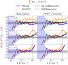 |
Fig. 3. Relative percentage difference of the nonlinear power spectrum computed with various recipes with respect to the DEMNUni simulations for the case ∑mν = 0.16 eV. We note that here, contrary to the forecast analysis, and to be consistent with the DEMNUni simulations, we assume the total neutrino mass to be equally shared among the three neutrino species m1 = m2 = m3 = ∑mν/3. The left column shows the total matter power spectrum, while the right column shows the cold dark matter power spectrum. The spectra are evaluated at z = 0, 1, 2 (first, second and third rows, respectively). The theoretical predictions are provided by HALOFIT (dashed orange line), HMcode (solid blue line), EuclidEmulator2 (dashed red line), and BACCOemulator (dot-dashed green line). The purple shaded area represents the shot noise of the simulations, and the vertical dotted line the maximum wavenumber. In the third row the predictions of BACCOemulator are missing because the emulator is trained only up to z = 1.5. The predictions for the cold dark matter power spectrum (neglecting the contribution of neutrino perturbations) is computed according to the approximate formula Eq. (16) (see text for details). |
In our usage case, it is not only important to accurately model the clustering of the total power spectrum but also of the CDM+baryon power spectrum (see Sect. 3). In the right column of Fig. 3 we show the accuracy of the same nonlinear recipes in predicting the cold dark matter and baryons power spectrum Pcc(k, z) extracted from the DEMNUni simulations. In order to convert the nonlinear Pmm(k) into the nonlinear Pcc(k) we use the formula

where Pmm(k) is the total matter auto-correlation power spectrum, Pνν(k) the neutrino auto-correlation power spectrum, Pcν(k) the cross-correlation cold dark matter–neutrino power spectrum, fc the cold fraction of dark matter, and fν = (1 − fc) the hot one. The formula is correct as long as all the power spectra appearing both in the left-hand side and in the right-hand side are either linear or nonlinear. An approximation arises when mixing linear and nonlinear power spectra. Here we consider nonlinear Pmm(k) and Pcc(k), while Pcν(k) and Pνν(k) are assumed to be linear. This assumption is accurate for Pνν(k), because for ∑mν ≲ 0.6 eV the neutrino free-streaming length is larger than the nonlinear scale today (and even more so at higher redshifts). On the other hand, while we expect the cold dark matter–neutrino cross-power spectrum Pcν(k) to exhibit some nonlinearities, these are found to be negligible.
The right panel of Fig. 3 shows precisely the accuracy of this approximation: we compare results from the DEMNUni simulations against the nonlinear Pcc(k) of the various emulators obtained by inverting Eq. (16), where only Pmm(k) is assumed to be fully nonlinear. Concerning the accuracy on Pcc(k) of the different prescriptions adopted to compute the theoretical Pmm(k) [from which we derive Pcc(k)] the same considerations drawn for the total matter power spectrum hold true here. While HALOFIT fails to accurately reproduce the results of the simulations, the accuracy of the emulators is better than the one of HMcode, especially at low redshift. However, both HMcode and the emulators remain within 2% accuracy with respect to the DEMNUni simulations at any redshift and scale.
In Fig. 4, we show the massive neutrino (∑mν = 0.16 eV and ∑mν = 0.32 eV) induced suppression in the total matter power spectrum (left plot) and in the CDM+baryon power spectrum (right plot), with respect to a ΛCDM cosmology for the DEMNUni simulations and for the nonlinear predictions described above. For larger neutrino masses, HMcode outperforms not only HALOFIT but also the emulators in the precision of modelling this suppression. We note that a neutrino mass of about 0.3 eV, although it is excluded in the minimal ΛCDM + ∑mν scenario by the most stringent cosmological constraints to date (e.g. Alam et al. 2021; Palanque-Delabrouille et al. 2020), remains within reach in extended models (Lambiase et al. 2019).
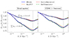 |
Fig. 4. Theoretical predictions of the suppression of the total matter power spectrum (left) and of the cold dark matter power spectrum (right) in massive neutrino cosmologies (∑mν = 0.16 eV and ∑mν = 0.32 eV) with respect to the pure ΛCDM case with massless neutrinos at z = 0. The colour coding of the theoretical predictions is the same as in Fig. 3. In the case ∑mν = 0.32 eV, EuclidEmulator2 is not shown because the value of the neutrino mass is too far away from the range of validity of the emulator. The DEMNUni simulations are depicted as black pluses. |
Finally, we are also going to vary the effective number of neutrino-like species (Neff) in our main analysis. To understand the nonlinear clustering in cosmologies in this case, we performed simulations with 10243 particles in a box with size L = 1024 h−1 Mpc varying Neff between 0.2 and 0.4. In Fig. 5 we checked the accuracy of HALOFIT, HMcode, EuclidEmulator2, and BACCOemulator with respect to these Neff simulations. The two emulators fail in reproducing the variations of the number of neutrino species (green and red lines, BACCOemulator and EuclidEmulator2, respectively); this was expected since they are not trained on cosmologies with non-standard Neff. In order to overcome the parameter extension with the emulators, we tried to remap the variation in Neff on large scales to a variation in the total matter and cold dark matter density parameters {Ωm, 0, Ωc, 0} and of the reduced Hubble constant h using the relationship derived in Rossi et al. (2015). However, tweaking the parameters does not improve the accuracy of the reconstruction of the Neff variations by means of emulators to a level competitive with HMcode. On the other hand, HMcode provides a good fit of the relative difference in the nonlinear clustering induced by variations of the number of neutrino-like particles, both for the phase-shift in the BAO scale, and for the overall suppression at small scales. Indeed, even though the HMcode parameters are not fit to simulations with varying Neff, the model is based on the convolution with the linear power spectrum, which naturally embeds the effect of Neff.
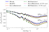 |
Fig. 5. Theoretical predictions of the suppression of the total matter power spectrum in non-standard Neff cosmologies with respect to the standard one, at z = 0, and assuming fixed values of {Ωm, 0, Ωb, 0, h}, like in the top panel of Fig. 2. The colour coding of the theoretical predictions is the same as in Fig. 3. We add here two more prescriptions, obtained by rescaling Ωc, 0, Ωb, 0 and h to mimic changes in Neff. We refer to it as “ΛCDM equivalent”: the dot-dashed pink line represents results for EuclidEmulator2; and the dotted cyan line represents the BACCOemulator prediction. Black crosses represent results from N-body simulations. |
To summarise, the emulators reach 1% accuracy in reproducing the CDM+baryon power spectrum in massive neutrino cosmologies out to k = 1 h Mpc−1, thus performing slightly better than HMcode, as already noted in Adamek et al. (2023). However, given their range of validity in terms of redshift (BACCOemulator) and neutrino mass (EuclidEmulator2) and especially given that they are not trained in varying Neff cosmologies, we opted for HMcode as our recipe to compute nonlinear corrections.
4. Additional probes
Through the history of the Universe neutrinos evolve from behaving like radiation to contributing to the total matter density. In order to capture neutrino effects at different epochs and remove parameter degeneracies, it is crucial to combine primary probes with additional secondary probes on larger scales from the Euclid survey, such as cluster number counts, and with external data probing the early Universe, such as from CMB anisotropies.
4.1. Cluster number counts from the Euclid survey
Clusters of galaxies are potentially a strong cosmological probe (Oukbir & Blanchard 1997; White et al. 1993; Bahcall & Fan 1998; Reiprich & Boehringer 2002; Mantz et al. 2008; Vikhlinin et al. 2009). Measurements of their abundance and evolution allow us to place constraints on both the geometry of our Universe and the growth of its density perturbations (Mohr 2005; Vikhlinin et al. 2009; Allen et al. 2011; Kravtsov & Borgani 2012). This could be achieved in particular from galaxy cluster number-counts experiments where, assuming that a halo number density mass function is predicted in a given cosmological model, one can confront the number of observed clusters computed in a given survey volume with its theoretical prediction and, from it, constrain cosmological parameters (Bocquet et al. 2019; Kirby et al. 2019; Costanzi et al. 2021; Sakr et al. 2022; Lesci et al. 2022). Euclid will study galaxy clusters abundance, an independent and complementary probe to the two primary ones, allowing the optical detection of clusters previously unattainable in terms of the depth and area covered. Under optimistic assumptions about the calibration of the mass-observable relation, Carbone et al. (2012), Basse et al. (2014), Cerbolini et al. (2013), Sartoris et al. (2016) find that the promising increase in the number of detected clusters will provide tight constraints on models of dark energy or non-minimal massive neutrinos.
To forecast constraints from cluster number counts, we have followed a similar approach to Sartoris et al. (2016) on the modelling of the mass-observable scaling relation and selection function. The cluster’s mass is derived from a scaling relation with an observable quantity, such as the cluster richness, luminosity, velocity dispersion or shear from gravitational lensing. We call Mobs this mass. The estimated number counts of these clusters for a redshift bin l and mass bin m, corresponding to zl and Mobs, m, can then be expressed as
![$$ \begin{aligned} N_{l, m}& = \int _{\Omega _{\rm tot}} \mathrm{d} \Omega \int ^{z_{l+1}}_{z_l}\mathrm{d} z \;\frac{\mathrm{d} V}{\mathrm{d} z\,\mathrm{d} \Omega }\nonumber \\& \quad \times \int ^{+\infty }_0 \mathrm{d} M \; \frac{\mathrm{d} n(M,z)}{\mathrm{d} M} \frac{1}{2}\left[ \mathrm{erfc} (x_{m,l}) - \mathrm{erfc}(x_{m+1,l})\right], \end{aligned} $$](/articles/aa/full_html/2025/01/aa50859-24/aa50859-24-eq35.gif)
under the assumption of a log-normal observed mass distribution. Here dn(M, z)/dM is the cluster mass function of Euclid Collaboration (2023) defined below, dΩ is the solid angle element in steradians, dV/(dz dΩ) is the derivative of the comoving volume with respect to the redshift and solid angle element,
with DA(z) being the angular diameter distance and c the speed of light, while erfc(x) is the complementary error function, with the argument x being the (biased) logarithm of the mass (see below). We can explicitly write this as xm, l = x (Mobs, m, l) defined in each mass bin m and redshift bin l as
We define the bias and the variance to be
and

where BM, 0, bE, and αE are free parameters to quantify, respectively, the change in calibration, slope, and redshift dependence in the mass-observable-biased log-normal mass distribution, with Mpivot = 3 × 10¹⁴ h−1 M⊙, while σMobs, 02 and βE serve also to respectively calibrate and account for the redshift dependence in the variance. The predicted number density of halos of mass M at redshift z (the mass function) is given by
![$$ \begin{aligned} \frac{\mathrm{d} n(M,z)}{\mathrm{d} M} = \frac{\rho _{\mathrm{bc},0}}{M}\,\mathcal{F} \big [\sigma (R,z) \big ] \, \frac{\mathrm{d} \ln \big ( \, [\sigma (R,z) \big ]^{-1} \, \big )}{\mathrm{d} M}, \end{aligned} $$](/articles/aa/full_html/2025/01/aa50859-24/aa50859-24-eq40.gif)
where σ(R, z) is the variance of the density field within a sphere of radius R at redshift z, and it is computed following Costanzi et al. (2013) neglecting the massive neutrino component, from the linear CDM+baryon power spectrum Pcc(k, z) as
where W(kR) is the top-hat filter in k-space,
![$$ \begin{aligned} W(kR) = 3\frac{\left[\sin (kR)-kR\cos (kR)\right]}{(kR)^3}, \end{aligned} $$](/articles/aa/full_html/2025/01/aa50859-24/aa50859-24-eq42.gif)
R = R(M) = (3M/4πρbc, 0)1/3 is the radius of a sphere enclosing a mass M, and ρbc, 0 = ρcrit, 0 Ωbc, 0 is the mean CDM+baryon energy density at z = 0. Here we have used the critical density ρcrit, 0 and the CDM+baryon density fraction Ωbc, 0 = Ωm, 0 − Ων, 0. Finally, the multiplicity function reads, according to the modified Press–Schechter formalism of Euclid Collaboration (2023):
where ν(M, z) = δc(z)/σ(R, z), and δc(z) is the linear density contrast for spherical collapse. This can be computed following the prescription of Weinberg & Kamionkowski (2003):
![$$ \begin{aligned} \delta _{c, \mathrm{lin}}(z) \simeq \frac{3}{20} (12\pi )^{2/3}[1+0.0123 {{\,\mathrm{log_{10}}\,}}\Omega _{\rm m}(z)]. \end{aligned} $$](/articles/aa/full_html/2025/01/aa50859-24/aa50859-24-eq44.gif)
Note that this formula does not take into account any massive neutrino, except for Ωm. Here the matter density fraction Ωm(z) at redshift z is computed from the present day total matter density Ωm, 0 as
The redshift and scale-dependence of the parameters of Eq. (24) can be written as
![$$ \begin{aligned} A(p,q)&= \left\{ \frac{2^{-0.5-p+q/2}}{\sqrt{\pi }} \left[ 2^p \Gamma (q/2)+ \Gamma (-p+q/2) \right] \right\} ^{-1},\end{aligned} $$](/articles/aa/full_html/2025/01/aa50859-24/aa50859-24-eq46.gif)
![$$ \begin{aligned} q&= q_{\rm R} \, [\Omega _{\rm bc}(z)]^{q_z},\end{aligned} $$](/articles/aa/full_html/2025/01/aa50859-24/aa50859-24-eq47.gif)
![$$ \begin{aligned} q_{\rm R}&= q_1 + q_2 \left[ \frac{\mathrm{d} \ln \sigma (R,z)}{\mathrm{d} \ln R} + 0.5 \right],\end{aligned} $$](/articles/aa/full_html/2025/01/aa50859-24/aa50859-24-eq48.gif)
![$$ \begin{aligned} p&= p_1 + p_2 \left[ \frac{\mathrm{d} \ln \sigma (R,z)}{\mathrm{d} \ln R} + 0.5 \right],\end{aligned} $$](/articles/aa/full_html/2025/01/aa50859-24/aa50859-24-eq49.gif)
![$$ \begin{aligned} a&= a_{\rm R} \, [\Omega _{\rm bc}(z)]^{a_z},\end{aligned} $$](/articles/aa/full_html/2025/01/aa50859-24/aa50859-24-eq50.gif)
![$$ \begin{aligned} a_{\rm R}&= a_1 + a_2 \left[ \frac{\mathrm{d} \ln \sigma (R,z)}{\mathrm{d} \ln R} + 0.6125 \right]^2, \end{aligned} $$](/articles/aa/full_html/2025/01/aa50859-24/aa50859-24-eq51.gif)
where the parameters ai, pi, and qi are calibrated to the simulation. The adopted values of the seven fitted parameters are listed in Table 3.
The corresponding likelihood function is based on Poisson statistics (Cash 1979; Holder et al. 2001; Bonamente 2020):
![$$ \begin{aligned} \ln \mathcal{L} _{\rm CC} &= \ln \mathcal{P} (n_{l,m}|N_{l,m}) \nonumber \\& = \sum _{l=1}^{N_l}\sum _{m=1}^{N_m} [n_{l,m} \ln (N_{l,m}) - N_{l,m} - \ln (n_{l,m}!)], \end{aligned} $$](/articles/aa/full_html/2025/01/aa50859-24/aa50859-24-eq52.gif)
where 𝒫(nl, m|Nl, m) is the Poisson distribution probability of finding nl, m clusters given an expected number of Nl, m in each bin in redshift and mass. The Nl, m are computed from Eq. (17), whereas the nl, m are the fiducial values of the Nl, m. To estimate the number counts, we have considered equally spaced redshift bins in z ∈ [0.2, 1.8], with a width of Δz = 0.1. As for the limiting mass, we have followed the selection function used in Sartoris et al. (2016) in the pessimistic case where the lower mass for clusters is defined as the one corresponding to the significance of detection threshold, or the ratio between the cluster galaxy number count and the field RMS, Nc/σfield is above 5. In our analysis, we also conservatively vary the nuisance parameters. In order to compute the fiducial mocks the latter are set to (BM,0, bE, αE, σln,M,0, βE) = (0.0, 1.0, 0.0, 0.2, 0.125).
4.2. Cosmic microwave background
In Sect. 7 we forecast the sensitivity to neutrino parameters of the Euclid probes combined with CMB data from the Planck satellite. In the context of a forecast, it is easier to describe the Planck constraining power not through the actual data and likelihood, but through mock data and a synthetic likelihood mimicking the sensitivity of Planck. This allows us to assume the same underlying cosmology for our Euclid and Planck mock data, and perform our forecast in ideal conditions – of course, one should keep in mind that this is a very different exercise from a real data analysis, which can bring surprises, especially if different data sets are in tension due to statistical flukes, incomplete systematic modelling, or physical effects that have not been accounted for.
As in many previous works, we use for this purpose the fake_planck_realistic likelihood of the public MontePython package, which accounts for the measurement of CMB temperature, polarisation, and lensing by Planck, with a sky coverage of 57% and noise spectra very close to the actual ones. This Gaussian likelihood accounts for three correlated observables: the CMB temperature map; the E-mode polarisation map, and the reconstructed CMB lensing potential map. In principle, these observables are slightly correlated with Euclid observables because the same clusters can shear high-redshift Euclid galaxies and distort patterns on the last scattering surface. This correlation will be taken into account in the analysis of real Euclid data, but, for simplicity, we neglect it in the present forecasts.
Next, we estimate the potential of Euclid data in combination with future CMB data from the LiteBIRD satellite, optimised for large angular scales, and from the CMB Stage-IV survey (CMB-S4), optimised for smaller angular scales. As in Brinckmann et al. (2019) we model this combination with two mock likelihoods in the public MontePython package: the litebird_lowl likelihood accounts for LiteBIRD temperature and polarisation data in the multipole range where the survey is the most constraining, 2 ≤ ℓ ≤ 50; and the cmb_s4_highl likelihood for temperature, polarisation, and lensing data from CMB-S4 at ℓ > 50. Details on the assumed sensitivity can be found directly in the numerical package or in Brinckmann et al. (2019). In that case, we follow the same methodology as for Planck: the CMB mock data account for the same fiducial model as Euclid and we neglect correlations between the CMB and large-scale structure data, although this correlation will be more important for a survey very sensitive to CMB lensing like CMB-S4.
For CMB experiments, the predicted error on Neff depends mainly on the sensitivity of data to small angular scales. This means that in our modelling of LiteBIRD+CMB-S4 the assumptions regarding the CMB-S4 sensitivity at large ℓ are crucial. As in the rest of this forecast paper, we stick to conservative assumptions. Similarly to Brinckmann et al. (2019), we assume that foregrounds can be removed from CMB temperature and polarisation data only up to ℓmax = 3000, that the Galactic cut imposes a sky coverage fsky = 0.40, and that the CMB-S4 instrument can be modelled with a beam width of θ = 3.0 arcmin and a sensitivity to temperature of σT = 1.0 μK arcmin. With such assumptions, the combination of LiteBIRD+CMB-S4 predicts σ(Neff) = 0.038 in the ΛCDM+∑mν+Neff case – see Table 5 of Brinckmann et al. (2019). Since in this case the posterior is nearly Gaussian, this implies a 95% CL upper bound ΔNeff < 0.076. This is consistent with the forecasts of the CMB-S4 white paper Abazajian et al. (2016), but that paper explores many other assumptions on CMB-S4 data, with a maximum multipole for the temperature data in the range ℓmaxTT ∈ [3000, 5000], a sky fraction fsky ∈ [0.1, 0.8], a beam width of θ ∈ [1.0, 3.0] arcmin, and a sensitivity of σT ∈ [1.0, 3.0] μK arcmin – see Figs. 22–24 of Abazajian et al. (2016). We should stress that in that regard the summary plot of Fig. 23 (right panel) – which can be compared with our Fig. 18 – CMB-S4 forecasts are performed under extremely optimistic assumptions: ℓmaxTT = 5000, fsky = 0.5 (respectively 0.7), θ = 1.0 arcmin, and σT = 1.0 μK arcmin, which gives a 95% CL upper bound ΔNeff < 0.054 (respectively 0.046). While these numbers provide an example of what CMB Stage-IV may ideally achieve, we want to give more conservative estimates of what will be possible with the combined surveys.
5. Forecast method
Having described our modelling of observables and likelihood functions in Sects. 3 and 4, we now explain how such likelihoods can be used for the purpose of Euclid forecasts. Our forecast methods are based on Euclid Collaboration (2024a), adjusted to account for the presence of massive neutrinos. The validation of the four different pipelines described in this section against each other is detailed in Sect. 6 and one of them (i.e. the MCMC pipeline) was used in deriving our main results, presented in Sect. 7.
If the parameters are well constrained, we can approximate the posteriors with a multivariate Gaussian. Since such a distribution can be described by a mean vector and a covariance matrix, with such an approximation all the information concerning the sensitivity of the experiment to the parameters of the model is contained in the Hessian matrix Fαβ of the log-likelihood at the best fit, also called the Fisher Information (FI) matrix:

where the indices {α, β} run over model (cosmological or nuisance) parameters. Our version of the MontePython package implements mock likelihood functions ℒ(θα) for each of the Euclid probes described in Sect. 3. The pipeline referred to later as MP/Fisher (the MontePython package used in Fisher mode) directly evaluates the FI matrix from Eq. (34). First, the code calls the Einstein–Boltzmann solver (EBS) CLASS to evaluate the cosmological observables required by the likelihood calculation (power spectra, growth rate, etc.). Then, it performs a numerical calculation of two-sided second-order derivatives, based on the evaluation of the likelihood at the best fit and in 2N2 neighbouring points, where N is the number of model parameters12.
Due to the computational cost and complexity of evaluating second-order derivatives, one can use the fact that the likelihoods have a relatively simple Gaussian dependence on the power spectra (but not on the parameters) to express the Fisher matrix in terms of first derivatives only. For the photometric probe, the FI matrix can be expressed as
![$$ \begin{aligned} F_{\alpha \beta } = \frac{1}{2} f_\mathrm{sky} \sum _\ell (2\ell +1) \mathrm{Tr} \left\{ \left[\mathsf {C}^\mathrm fid\mathsf (\ell )\right]^{-1} \left[ \left. \partial _\alpha \mathsf {C}^\mathrm th\mathsf (\ell )\right|_\mathrm{fid} \right] \nonumber \right.\\ \left. \left[\mathsf{{C}^\mathrm fid\mathsf (\ell )}\right]^{-1} \left[\left. \partial _\beta \mathsf {C}^\mathrm th\mathsf (\ell )\right|_\mathrm{fid} \right] \right\} , \end{aligned} $$](/articles/aa/full_html/2025/01/aa50859-24/aa50859-24-eq54.gif)
where for each multipole ℓ the matrices Cfid and Cth are built out of the angular power spectra  defined in Eq. (4), evaluated, respectively, at fiducial parameter values in the case of Cfid, or at two points (per dimension) in parameter space to compute numerically the first-order derivative
  . Since with this method only the first-order derivatives are evaluated, the total number of points needed reduces to 2N (using a first-order double-sided finite difference). We refer the reader to Euclid Collaboration (2024a) for more details on the definition of the matrices Cfid and Cth. For the spectroscopic probe, the FI matrix becomes instead
![$$ \begin{aligned} F_{\alpha \beta } &= \sum _i \frac{1}{8\pi ^2} \int _{-1}^{1} \mathrm{d} \mu \int _{10^{-3}}^{k_{\rm max}} \mathrm{d} k\, k^2\, ~ \left[\partial _\alpha \mathrm{ln} (P_\mathrm{obs} )\big |_\mathrm{fid} \right.\nonumber \\& \quad \times \left. \partial _\beta \mathrm{ln} (P_\mathrm{obs} )\big |_\mathrm{fid} V_i^\mathrm{fid} \right], \end{aligned} $$](/articles/aa/full_html/2025/01/aa50859-24/aa50859-24-eq57.gif)
where Pobs is the observable power spectrum defined in Eq. (11), kmax is given in Table 2 and the index i runs over four redshift bins with effective volume Vifid. Details on the assumed survey characteristics and binning strategy are specified in Euclid Collaboration (2024a).
The pipeline that we refer to as CF, that is, the CosmicFish code, uses Eqs. (35) and (36) to compute the FI matrix. It calculates the matrices C(ℓ) and the spectra Pobs at the fiducial point and at a given number of neighbouring points in parameter space, and numerically evaluates the first derivatives of these observables with respect to model parameters. By default, CosmicFish uses two-sided first-order derivatives (two neighbouring points). To check the numerical stability of this method, we have checked that we get similar result when using a 4-point forward stencil derivative (see Appendix A). The version of CosmicFish used in this work internally calls one of the EBSs (CAMB or CLASS ) to evaluate the cosmological observables, providing us with two forecast pipelines CF/CAMB and CF/CLASS13.
Our fourth pipeline called MP/MCMC is the MontePython package used in its default mode, which is running Markov chain Monte Carlo (MCMCs) with a Metropolis-Hasting algorithm to explore the parameter space and infer the posterior from the likelihood according to Bayes theorem. We always assume top-hat priors on model parameters, with prior edges chosen far in the exponential tails of the posteriors, such that the confidence intervals inferred from the MCMCs at the 95% CL are unaffected by the choice of prior edge. The only exception is the summed neutrino mass ∑mν, for which we impose a theoretical prior ∑mν > 0. The two main advantages of MCMC forecasts is that they rely neither on a Gaussian approximation to the likelihood, nor on the calculation of numerical derivatives. We note that the MP/Fisher and MP/MCMC pipelines call the very same Euclid mock likelihoods, computing the same functions ℒ(θα), which are the only parts of the pipeline depending on the cosmology; thus, it is impossible by construction to introduce a mistake in the modelling of cosmology (or of the Euclid survey) when passing from one pipeline to the other. This means that the validation of one pipeline automatically implies the validation of the other pipeline (as long as the FI matrix is well conditioned and the MCMC has converged).
This statement could be questioned in the case in which one of the two approaches (FI matrix or MCMC) requires a more accurate calculation of the cosmological observables or of the likelihood functions. In the case at hand, we know that the highest precision is required by the FI matrix approach, because a robust evaluation of numerical derivatives with small step sizes requires high accuracy and low numerical noise. However, our approach consists of validating the MP/Fisher pipeline first, which is more demanding in terms of accuracy; this in turn validates the MP/MCMC pipeline, which is less demanding. We also explicitly compare the results from the two pipelines in Sect. 6 to make sure that they agree.
6. Code validation
In order to validate the four forecast pipelines described in Sect. 5 against each other, we need to choose a framework (fiducial model and set of parameters) in which the FI formalism can be applied in a robust way. In the results section, we will be interested in extensions of the minimal five-dimensional (5D) flat ΛCDM model with up to four additional free parameters {∑mν, Neff, w0, wa}14. However, floating these nine parameters simultaneously opens up strong degeneracies in the parameter space and leads to very non-Gaussian posteriors. In that case, the Gaussian approximation breaks down. Then, the FI matrix calculation becomes unstable, since it depends heavily on the choice of numerical derivative step sizes. Besides, the FI matrix no longer provides a good estimate of the experimental sensitivity.
To overcome this issue, we decided to validate our forecasting pipelines by looking separately at three 7-parameter models for which the posterior remains close to Gaussian (as confirmed by contour plots from MCMC runs displayed in Sect. 6.2). This strategy does not limit the range of validity of our final results, since at the end, after validating the pipelines against each other, we will use the MCMC pipeline for our main results. This pipeline does not rely on any Gaussian approximation and can be used even for full 9-parameter forecasts.
The three seven-parameter models used for validation are defined as follows. Firstly, we stick to a w0waCDM cosmology, with a time-varying dark energy equation of state parameter w(a) = wa(1 − a)+w0 (Chevallier & Polarski 2001; Linder 2003) but fixed {∑mν, Neff}. This model was already used in the forecasts of Euclid Collaboration (2024a) and allows us to cross-check that the previous validation still holds. Secondly, we investigate cosmologies where we vary the neutrino mass and the effective number of relativistic degrees of freedom, ΛCDM+∑mν+Neff, but stick to a cosmological constant. This framework allows us to cross-check our implementation on neutrino effects on the observables. Thirdly, we consider models with varying neutrino mass and dark energy equation of state, w0CDM+∑mν, with fixed Neff = 3.044 and wa = 0. This last set up will prove that our modelling of nonlinear corrections is consistent across the different pipelines even when neutrino and DE parameters are varied simultaneously.
The fiducial values of cosmological parameters used in Sects. 6 and 7 are summarised in Table 4. Despite identical fiducial values, the models used for validation in this section and for forecasts in the next section feature two subtle differences with respect to each other. First, as already explained in Sect. 2.2 (case b), we assume here a single massive neutrino species with mass mν = ∑mν, which allows for easier comparison with earlier work and for simpler FI matrix calculations (given that the Neff posterior remains symmetric around the fiducial value). Second, we fix here the nonlinear modelling parameters σp and σv to their fiducial values in order to keep the contours of the spectroscopic probe more Gaussian. In Sect. 7, we instead consider three degenerate massive neutrino species, each with mass mν = ∑mν/3 (see Sect. 2.2, case a) and we will marginalise over σp and σv.
Fiducial values of the cosmological parameters used in the validation and result sections.
We performed validation tests for each of the three seven-parameter models, each probe (photometric or spectroscopic), and each case (pessimistic or optimistic). Thus, the number of validation tests amounted to 12. In each of these 12 situations, we proceeded as follows:
-
Validate the predictions and accuracy settings of the EBSs by comparing the CF/CAMB and CF/CLASS pipeline results;
-
Validate our MontePython likelihood and our FI matrix implementation by comparing the results from the CF/CLASS and MP/Fisher pipelines;
-
Check the validity and stability of our FI forecasts (choice of step size in numerical derivatives and validity of Gaussian approximation) by comparing the previous two pipelines with MP/MCMC runs.
In practice, we performed steps 1 and 2 simultaneously, by comparing all three derived FI matrices. For steps 1 and 2, our test consisted of comparing the marginalised and unmarginalised errors on each cosmological and nuisance parameter15. Validation was achieved when all errors were within 10% of the median. This subjective criterion16 was already adopted in previous Euclid validation papers like EC20 and Euclid Collaboration (2024a). The results of these tests are shown in Sect. 6.1. For step 3 we compared 1D posteriors and 2D confidence contours in triangle plots in Sect. 6.2.
6.1. Validation of Fisher pipelines
We show the marginalised and unmarginalised errors predicted by each pipeline (CF/CAMB, CF/CLASS, MP/Fisher) used to compute the FI matrix, each probe, and each case, respectively, in Fig. 6 for the w0waCDM model, in Fig. 7 for the ΛCDM+∑mν+Neff model, and in Fig. 8 for the w0CDM+∑mν model. In all cases, the errors are within 10% of the median, leading to the validation of the pipelines.
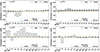 |
Fig. 6. For the w0waCDM model, comparison of each of the Fisher marginalised (light grey) and unmarginalised (dark grey) errors on each cosmological and nuisance parameter for: photometric optimistic probe (top left); photometric pessimistic probe (top right); spectroscopic optimistic probe (bottom left); and spectroscopic pessimistic probe (bottom right). For the spectroscopic probe the labels lbsi are short for the parameters ln(b σ8)i. |
Uncertainties from CF/CAMB and CF/CLASS are usually within 2% of each other, which shows the excellent agreement between the two EBSs. Such a level of agreement was achieved after a careful setting of the parameters describing underlying assumptions on the cosmological models (especially those controlling the modelling of the neutrino sector) and of accuracy settings. Our choice of input and accuracy settings for CAMB and CLASS is described in Appendix B. The errors from CF/CAMB and CF/CLASS differ by more than 2% only in the photometric case, in which the σ8 and ∑mν errors are 3–5% away from each other. We believe this is due to the tiny but irreducible difference in the neutrino treatment between CLASS and CAMB. As shown in Fig. B.1, the suppression of the power spectrum on small scales due to neutrinos seems to start earlier in CLASS than CAMB, inducing differences of the order of 0.1% in the linear matter power spectrum. Still, the final error bars achieve a level of agreement that is remarkable and sufficient for Euclid purposes.
Errors from CF/CLASS and MP/Fisher are within 10% of each other. The precise level of agreement is sensitive to the choice of step sizes, especially in the MP/Fisher pipeline. For this choice, we adopted the following strategy
-
For CF/CAMB and CF/CLASS, we adopt by default relative steps of 1% in each parameter (or 0.01 for wa). However, we observed that this choice is inappropriate for ∑mν, since this parameter has a smaller impact on the matter power spectrum. The effect of a 1% variation in the neutrino mass on both Pmm and Pcc is so small that numerical derivatives would be dominated by numerical noise from the EBSs. Thus, for ∑mν, we adopt a step size of 10%, that is, Δ(∑mν) = 6 meV. We checked that the results are relatively stable against small variations in the step sizes (see Appendix C) and against a change in the numerical derivative method (see Appendix A).
-
In MP/Fisher, we stick to the recommendation of Euclid Collaboration (2024a) and choose the step size in relation to the marginalised 1D parameter uncertainty for each individual parameter for a given model. To get the uncertainties, we could either run an MCMC or use the error obtained from CosmicFish. In this case we use the uncertainties obtained from CosmicFish. In the case of the photometric probe, we choose a step size of 10% of the posterior error, while for the spectroscopic probe, we used a step size of 5% of the error.
These results are very sensitive to the modelling of nonlinear corrections. In Sect. 3.3, we argue that the most recent version of HMcode (Mead et al. 2021) reproduces simulations featuring massive neutrinos significantly better than HALOFIT (Takahashi et al. 2012; Bird et al. 2012). We checked that using HALOFIT instead of HMcode does affect the marginalised forecasted errors by a large factor of 1.5 (see Appendix D). The assumption that galaxies trace cold-plus-baryonic matter instead of total matter is also important for Euclid, but to a lesser extent. When replacing Pcc by Pmm everywhere in the spectroscopic likelihood, the uncertainties vary by at most 5% on ∑mν (for our fiducial value ∑mν = 60 meV) (as shown in Appendix E).
6.2. Comparison of Fisher ellipses and MCMC contours
For each of the three validation models and each of the two probes, we show the 1D marginalised posteriors and the 2D marginalised confidence contours of our MP/MCMC runs in the triangle plots of Figs. 9 to 11. For this test, we only consider the optimistic case, which is the most sensitive to details in the modelling of the observables, and the most likely to reveal possible discrepancies in the numerical implementation of the likelihoods. This case is also the most constraining, and thus closer to the Gaussian approximation and the most suited for comparison with FI matrix predictions. In Figs. 9 to 11, we actually plot the Gaussian posteriors and elliptical contours of the CF/CAMB and MP/Fish pipelines on top of the MP/MCMC results.
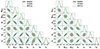 |
Fig. 9. Comparison of the 1D marginalised posteriors and 2D (95% C.L. and 68% C.L.) marginalised contours obtained with the MP/MCMC pipeline to the Gaussian posteriors and elliptical contours from the FI pipelines CF/CAMB and MP/Fisher for the w0waCDM model. Left: Spectroscopic optimistic probe. Right: Photometric optimistic probe. |
First and foremost, we can see in Fig. 9 that the previous validation of photometric probes presented in Euclid Collaboration (2024a) for the w0waCDM model is reproducible, despite the changes in the likelihood code and nonlinear recipe triggered by the assumption of massive neutrinos. Concerning the spectroscopic probes, here we have corrected for an inconsistency in the unit conversion from Mpc−1 to h Mpc−1 that affected previous forecasts; thus, the sensitivity to h degrades with respect to Euclid Collaboration (2024a), while the sensitivity to the other cosmological parameters is only mildly altered due to their correlations with h. Nevertheless, the conclusions drawn in Euclid Collaboration (2024a) about the validation of MP/MCMC for this case still hold: the posteriors of the photometric and spectroscopic probes are very close to multivariate Gaussians. We get another confirmation of this, since the MCMC and FI posteriors or contours are hardly distinguishable by eye and agree up to typical MCMC convergence errors.
In the case of the ΛCDM+∑mν+Neff model, we see in Fig. 10 that non-Gaussian effects come into play. This is particularly obvious when looking at the marginalised neutrino posteriors, which are truncated at ∑mν = 0 by the physical prior, and whose tails fall quicker than a Gaussian distribution for large masses. This non-Gaussianity propagates to the parameters that are most correlated with ∑mν. Indeed, the orientation of the 2D contours shows that h, Ωm, 0, ns, and σ8 are significantly correlated with ∑mν, while Ωb, 0 and Neff are not. The former parameters are also the ones whose posteriors deviate the most from a Gaussian shape. The fact that the MCMC contours are overall tighter than the FI ellipses is also a consequence of the non-Gaussianity with respect to ∑mν > 0, which cuts off a region of the parameter space (with either negative or too large neutrino mass) that would otherwise be reachable by FI contours. Deviations from Gaussianity are found to be even stronger within the photometric probe, both because the neutrino mass posterior is more suppressed for large masses and due to the very strong correlation between ∑mν, Ωm, 0, and σ8.
Finally, in the case of the w0CDM+∑mν model, we see some qualitatively similar trends in Fig. 11. For the spectroscopic probe, we observe a ‘banana’-shaped contour in the ns-∑mν plane and slightly non-elliptic contours in other planes. Once again, the non-Gaussianity is even more pronounced with the photometric probe, due to the cut-off of negative or too large neutrino masses.
As in Sect. 5, we stress that the MP/Fisher and MP/MCMC pipelines call the very same Euclid mock likelihoods functions ℒ(θα). Given that these functions have been validated by the tests presented in the previous subsection, and that the MCMC runs presented here have reached a high convergence level, the difference between the MCMC and FI contours can only be attributed to the intrinsic non-Gaussianity of the problem. This shows that for extended cosmological models, particularly in the case of a free neutrino mass parameter, robust Euclid forecasts (and even more so with respect to analyses of future real data) require a full MCMC analysis. Having validated the MontePython likelihoods against CosmicFish forecasts, we have proved that our MP/MCMC pipeline offers a robust and accurate implementation of the physical assumptions performed in this work. Thus, we can use it in the next section in order to derive our main forecast results.
7. Results
Here, we present the results of our forecast analysis. We use the previously validated MP/MCMC pipeline based on the MontePython sampler, interfaced with the Boltzmann solver CLASS. The underlying cosmology is either flat ΛCDM with the standard cosmological constant or w0waCDM, where dark energy is a fluid with a time-varying equation-of-state parameter according to Chevallier & Polarski (2001) and Linder (2003).
As already explained in Sect. 2.2 (case a), from the many possible ways of distributing the total mass ∑mν among the different species contributing to the effective number of neutrinos Neff (which could lead to potentially different results), we made a choice that is representative of a large class of well-motivated scenarios. We assume that the three active neutrino species are degenerate in mass with a fiducial value ∑mν = 60 meV close to the minimum allowed by normal ordering. We further assume that massive neutrinos contribute to Neff through the standard value 3.044 and that additional free-streaming massless particles account for ΔNeff = Neff − 3.044, with ΔNeff > 0 (see Appendix B.1 for details on the specific settings in CLASS and CAMB). Sticking to these assumptions, we consider four extended cosmological scenario with an increasing number of free parameters:
-
ΛCDM + ∑mν (baseline);
-
ΛCDM + ∑mν + ΔNeff;
-
w0waCDM + ∑mν;
-
w0waCDM + ∑mν + ΔNeff.
In Table 4 we list the fiducial values for the parameters of our models.
Here (in contrast to the validation of the MCMC pipeline) we use pessimistic specifications, additionally also varying the nonlinear nuisance parameters σv and σp of the GCsp recipe. The reasoning behind this choice is that additional theoretical errors and systematic effects might have been overlooked in the modelling of the observables adopted in EC20 and Euclid Collaboration (2024a). Therefore, applying optimistic specifications might overestimate the sensitivity to the neutrino mass, while our aim is to provide a conservative forecast of the Euclid discovery potential. Moreover, the cut-off at ℓmax = 1500, implied by pessimistic specifications, prevents our results from being biased due to the uncertainties on the modelling of baryonic feedback, as we discuss in Appendix H.
We fit both Euclid and CMB synthetic data (for the latter, see Sect. 4.2). For Euclid, the observables are the 3 × 2pt angular power spectra from photometric data (photometric galaxy clustering, weak lensing, and their cross-correlation, see Sect. 3.1), the 3D galaxy power spectrum from spectroscopic data (Sect. 3.2), and cluster number counts (CC, Sect. 4.1).
The cosmological parameter fiducial values were already specified in Table 4. The parameters w0 and wa are kept fixed to the fiducial value when the underlying cosmological model is ΛCDM. The parameters of the baseline model are always varied, while the parameters of the extended models (such as the number of relativistic degrees of freedom and the dark energy equation of state parameters) are kept fixed, unless specified. The optical depth to reionisation is fixed to the Planck best fit value τ = 0.0543 when only Euclid observables are included in the analysis, while we allow it to vary in the joint analysis with CMB probes.
In Table 5, we show the 1 σ uncertainty (or the 95% CL upper limit) on each cosmological parameter inferred from our MCMC forecasts, assuming different cosmological models and varying the combination of synthetic data17. In Fig. 12, we show the same results expressed in terms of a dimensionless sensitivity, which is the 1 σ uncertainty relative to the fiducial value18. In each panel we compare the two underlying cosmologies, which are ΛCDM + ∑mν (solid colour bars) and w0waCDM + ∑mν (hatched colour bars). The effective number of neutrino species is additionally varied in the bottom panel. The different colours show the sensitivity of three different data combinations: WL+GCph+XCph+GCsp (blue); Euclid +Planck (orange); and Euclid +CMB-S4+LiteBIRD (green).
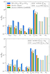 |
Fig. 12. Sensitivity (relative errors with respect to the fiducial values) to the cosmological parameters, comparing ΛCDM cosmologies (solid colour bars) and w0waCDM cosmologies (hatched colour bars), for models with (bottom panel) and without (top panel) varying Neff. The different colours correspond to the sensitivity of different data combinations: WL+GCph+XCph+GCsp (blue); Euclid +Planck (orange); and Euclid +CMB-S4+LiteBIRD (green). We note that for wa we show the absolute errors, while for ΔNeff we show the 95% upper limits. For the neutrino mass we always show the relative 1 σ uncertainty as computed from the posterior variance in order to facilitate the comparison between different data sets. |
Marginalised 1 σ uncertainties on cosmological parameters in ΛCDM + ∑mν, in ΛCDM + ∑mν + Neff, in w0waCDM + ∑mν, and in w0waCDM + ∑mν + ΔNeff.
Comparison with previous forecast. When comparing the results of the present forecast to those of EC20, one has to consider that we assume the same specifications labelled as pessimistic there. However, our baseline case includes the variation in the neutrino mass, which was not done in EC20. In light of these considerations, we observe that the sensitivity of the photometric probes (WL+GCph+XCph) to w0 and wa is consistent with the previous Euclid forecast from Table 11 of EC20 (note that they cite relative sensitivities, while we cite absolute sensitivities). On the other hand, the sensitivity to the other cosmological parameters degrades because of the correlation with the neutrino parameters; for example, the sensitivity to σ8 degrades by a factor of 1.6 in w0waCDM+∑mν+ΔNeff due to the free neutrino mass, while varying ΔNeff does not have any impact. A direct comparison of the results that include GCsp with those of EC20 is not feasible because, as already mentioned in Sect. 6.2, here we have corrected an inconsistency in the unit conversion from h Mpc−1 to Mpc−1 that was present in the pipeline of EC20. This issue produced a fake signal on H0, and, thus, a spurious enhancement of the sensitivity to h, which affected also the sensitivity to other cosmological parameters that are correlated with h. Note that we checked that reintroducing the bug would make our results consistent with those of EC20. Our results are also consistent with the older Euclid -like sensitivity forecast of Audren et al. (2013), which predicted a 1 σ sensitivity to ∑mν of 32 meV for Euclid WL + Planck or 25 meV for Euclid GCsp + Planck, while we obtain 23 meV for the combined WL + GCph + XCph + GCph + Planck data set. Interestingly, to account for the imperfect modelling of nonlinear scales, that forecast included a marginalisation over a theoretical error smoothly growing towards smaller scales, instead of cutting the data abruptly at some kmax or ℓmax like in the present work. Audren et al. (2013) adopted a theoretical error amplitude suggested by the covariance of the nonlinear power spectra predicted by different N-body codes for the same cosmology. The fact that our results are comparable suggests that their theoretical error and our pessimistic settings are equally conservative. A slightly different modelling of the theoretical error in Sprenger et al. (2019) led to a sensitivity to ∑mν of 24 meV for Euclid GCsp + WL + Planck with pessimistic specifications (there labelled as conservative), consistent with our results. Other works in the literature present Euclid -like forecasts (Yankelevich & Porciani 2019; Chudaykin & Ivanov 2019; Sailer et al. 2022) including only galaxy clustering with a one-loop modelling. However, the differences in assumptions, methodologies, and survey specifics make direct comparisons challenging.
Complementarity of Euclid probes. In Fig. 13, we show the constraints on the extended w0waCDM+∑mν+ΔNeff model expected from Euclid-only probes. The same figure for the baseline model ΛCDM + ∑mν can be found in Appendix F. We note that in the extended w0waCDM+∑mν+ΔNeff model the constraints on h and ΔNeff are dominated by the spectroscopic probes and those on σ8, ∑mν, w0, and wa by the photometric probes. The complementarity of the photometric and spectroscopic probes is impressive: the GCsp contours exhibit parameter degeneracies in different directions than the WL+GCph+XCph ones in several planes of the parameter space. In particular, the correlations between the dimensionless Hubble constant h and some of the other cosmological parameters that are present in GCsp are broken by the photometric information. This leads to a remarkable sensitivity increase in the joint analysis of the two primary Euclid probes.
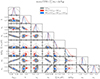 |
Fig. 13. Marginalised 1D distribution (diagonal) and 2D (off-diagonal) 68% and 95% contours for a selection of parameters of the w0waCDM+∑mν+Neff model obtained by fitting GCsp (grey), WL+GCph+XCph (red), and their combination (blue). The horizontal and vertical dashed lines mark the fiducial values. |
As far as the total neutrino mass is concerned, photometric probes are potentially more powerful than spectroscopic ones in constraining ∑mν. As long as we are not including CMB information, the observable effect of the total neutrino mass is best described by the top panel of Fig. 1, that is, a steplike suppression of the matter and cold-plus-baryonic power spectra. The longer lever arm of WL data thus provides the best constraint. However, the Euclid probes alone cannot provide significant evidence for a non-zero neutrino mass, neither in the w0waCDM cosmology (∑mν ≲ 0.22 eV, 95% CL, see Table 5) nor in ΛCDM [σ(∑mν) = 56 meV, see Table 5].
When using CMB data, there is a well-known correlation between ∑mν and h, due to their opposite effects on the angular diameter distance to last scattering. This strong correlation does not show up when fitting Euclid probes alone, mainly thanks to the sensitivity of galaxy clustering data to the unique scale dependence of the growth factor induced by massive neutrinos. Note that this conclusion does not depend on the specific underlying cosmological model, whether it is ΛCDM or w0waCDM, and whether ΔNeff is varying or fixed. We anticipate that the different directions of degeneracy between ∑mν and h in Euclid and CMB probes will induce a significant improvement on the ∑mν constraints in the Euclid +CMB joint analysis. Finally, note that we do not find any specific correlation between the neutrino mass and the bias parameters, neither in GCph nor in GCsp, as we show in Appendix G.
Concerning dark radiation, as already mentioned, a variation in ΔNeff impacts the matter and cold-plus-baryonic matter power spectra both through a change in the overall shape (caused by a shift of the time of equality) and in the phase and amplitude of BAO peaks (due to neutrino drag), as can be checked in the top panel of Fig. 2. The first effect induces a correlation between ΔNeff and h, since both parameters can be increased while maintaining a fixed redshift of equality. This correlation, combined with the prior volume effect induced by the physical prior ΔNeff > 0 (Hadzhiyska et al. 2023), leads to a small bias in the mean value of h and of ns reconstructed from photometric probes. We have explicitly checked that this bias disappears in the models where ΔNeff is fixed. The Euclid constraints on ΔNeff are dominated by the spectroscopic probe, because GCsp data partially break the correlation between ΔNeff and h thanks to a better measurement of BAO peaks. Nevertheless, the photometric probes contribute to the ΔNeff constraints by breaking the degeneracy in the ∑mν versus ΔNeff plane. Normally, one would expect a negative correlation between these parameters, due to their opposite effects on the BAO peak scale19. This negative correlation is clearly visible on the GCsp-alone contour of Fig. 13. Thanks to the large lever arm of WL data, the photometric probe allows us to distinguish the difference in overall shape and growth rate induced by variations of ∑mν or ΔNeff in the matter and cold-plus-baryonic power spectra, and to lift the degeneracy. As a consequence, a combination of the probes improves the sensitivity to both ΔNeff and ∑mν.
On the other hand, under our assumptions concerning the modelling of the Euclid cluster count data and likelihood, we find no significant improvement on cosmological parameter sensitivity when adding clusters. Table 5 shows the result for WL+GCph+XCph+GCsp+CC, where CC stands for cluster count, in the ΛCDM+∑mν and w0waCDM+∑mν+Neff cases. The difference between the results with and without CC lies within MCMC convergence errors. Additionally, in the w0waCDM+∑mν+Neff case, the upper bound on ΔNeff gets a tiny enhancement from a Bayesian prior volume effect related to small parameter degeneracies between ΔNeff and the nuisance parameters of the CC likelihood. We recall that we performed a very conservative modelling of CC data with wide priors on several nuisance parameters. With a more optimistic modelling, the same data may lead to tighter constraints.
Combination with CMB. In Figs. 14 and 15, we show the constraints placed on the parameters of the w0waCDM+∑mν+ΔNeff and ΛCDM+∑mν models for the combination of Euclid probes with CMB experiments, Euclid +Planck (orange contours), and Euclid +CMB-S4+LiteBIRD (green contours). The same figure for the other cosmological models can be found in Appendix F. These figures show that the Euclid probes will play a crucial role in improving constraints on the cosmological parameters considered in this work. As a matter of fact, we can identify several cases in which future CMB data sets allow for parameter degeneracies that are broken by Euclid probes.
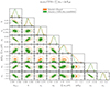 |
Fig. 14. Marginalised 1D distributions (diagonal) and 2D (off-diagonal) 68% and 95% contours for a selection of parameters of the w0waCDM+∑mν+Neff model obtained by fitting Euclid +Planck (orange), and Euclid +CMB-S4+LiteBIRD (green). The horizontal and vertical dashed lines mark the fiducial values. |
This is particularly true for the degeneracy between ∑mν and h. We already discussed above why these parameters are correlated in a CMB-only analysis, and why the Euclid probes can break this degeneracy, as can be checked again by comparing the {∑mν, h} panel of Fig. 13 with the same panel in Fig. 14 (see also Fig. 15). Additionally, when CMB data are taken into account, the observable impact of the total neutrino mass is best described by the bottom panel of Fig. 1, and amounts mainly to an overall (redshift-dependent) suppression of the matter and cold-plus-baryonic power spectra. Then, the role of CMB data is to fix the amplitude of the primordial spectrum of fluctuations at high redshift (modulo some uncertainty on the optical depth to reionisation that depends on CMB polarisation measurements on large angular scales), while the Euclid WL probe fixes the amplitude of the matter and cold-plus-baryonic power spectra at low redshift. Therefore, the combination of Euclid and CMB complementary data yields much stronger bounds on ∑mν than either of the two data sets taken separately, allowing eventually for a neutrino mass detection. Even in the minimal hierarchy scenario, which we assume as our fiducial model, the joint Euclid plus Planck forecast returns a 2.6 σ evidence for a non-zero mass with σ(∑mν = 60 meV) = 23 meV (Euclid +Planck). Finally, replacing Planck with a combination of future CMB surveys leads to the detection of a non-zero neutrino mass at almost 4 σ with σ(∑mν = 60 meV) = 16 meV (Euclid +CMB-S4+LiteBIRD). One of the reasons behind this improvement is the tightening of the constraints on the reionisation optical depth from LiteBIRD. Indeed, Fig. 16 shows how the joint fit of LSS and CMB data leads to a strong degeneracy between ∑mν and τ (Allison et al. 2015; Archidiacono et al. 2017). Therefore, the sensitivity to the neutrino mass can be further improved by means of an independent measurement of the reionisation optical depth. Such measurement can arise from future 21-cm experiments (Sailer et al. 2022)20, from probing the kinetic Sunyaev-Zeldovich effect in the CMB (Park et al. 2013), and from CMB polarization (Allys et al. 2023).
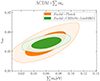 |
Fig. 16. Marginalised 2D contours of ∑mν and τreio for the ΛCDM+∑mν model. |
Given the fantastic ability of Euclid to constrain the neutrino mass sum in combination with CMB data, it is worth investigating whether Euclid data will help to reconstruct the neutrino mass hierarchy. Figure 17 shows the neutrino mass sum required by the two neutrino mass ordering schemes as a function of the mass of the lightest neutrino. We see that, if the neutrino mass sum has indeed the minimum value allowed by neutrino oscillations in normal ordering (NO), which coincides with the fiducial value of our forecast (∑mν = 60 meV), then the Euclid +CMB-S4+LiteBIRD sensitivity to the neutrino mass sum will also imply a 2.5 σ indication in favour of NO. Of course, the statistical significance of the evidence in favour of NO will decrease if the best-fit neutrino mass turns out to be larger than the minimum value of NO. It is important to stress that this measurement is not a direct probe of the neutrino mass ordering, but rather a consequence of the strong sensitivity to ∑mν.
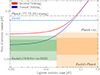 |
Fig. 17. Sum of neutrino masses ∑mν in the inverted ordering (red solid line) scenarios and in the normal ordering (blue solid line), including the uncertainties on the mass squared differences from oscillation experiments, as a function of the lightest neutrino mass. The grey dot-dashed lines show the 95% CL upper bounds from Planck only (dark grey), and in combination with external data (Planck +ext., light grey). For the latter we use the value quoted in Alam et al. (2021) for Planck +Pantheon-SNe+SDSS(BAO+RSD)+DES 3 × 2pt, which includes Planck, Pantheon type Ia supernovae, baryon acoustic oscillations and redshift-space distortions from the Sloan Digital Sky Survey, and weak lensing measurements from the Dark Energy Survey. The region above the blue dashed line is excluded at 95% CL by Euclid only primary probes. The orange shading shows the 68% and 95% CL limits on ∑mν from Euclid +Planck in the baseline ΛCDM+∑mν model, assuming a fiducial value ∑mν = 60 meV. The 68% and 95% CL constraints from Euclid +CMB-S4+LiteBIRD are shown in green. We note that we split the two constraints into two different ranges of the lightest neutrino mass only to avoid an overlap of the two shadings. Assuming that the true value of the neutrino mass sum is indeed the minimum allowed by neutrino oscillation experiments in normal ordering, the combination Euclid +CMB-S4+LiteBIRD will rule out the inverted ordering at 2.5 σ. |
Contrary to the case of ∑mν, the constraints on ΔNeff are dominated by CMB probes. Nevertheless the Euclid probes play an important role in breaking some of the degeneracies with other cosmological parameters, and in particular between ΔNeff and h. Euclid improves the Planck sensitivity to the Hubble constant by a factor of 2.5 (σ(h) = 0.0021, Euclid +Planck, in ΛCDM+∑mν, compared with Table 2 of Planck Collaboration VI 2020); as already discussed and shown in Fig. 13, this is mainly due to GCsp data. This significantly increases the sensitivity of combined CMB and Euclid data to ΔNeff. Additionally, as shown in the bottom panel of Fig. 2, once we include CMB information (thus fixing the angular size of the sound horizon at recombination), an increase in Neff leads to an enhancement of the matter and cold-plus-baryonic power spectra at small scales. This effect provides additional sensitivity to Neff. Figure 18 shows that adding Euclid improves the current limit (Planck Collaboration VI 2020) on the presence of new light particles by more than a factor of 2 (ΔNeff < 0.144, 95% CL, Euclid +Planck, in ΛCDM+∑mν+ΔNeff). On the longer term, the Euclid probes even have the potential to improve the sensitivity of future CMB data sets like LiteBIRD+CMB-S4 to Neff – once more, not because of a better sensitivity to the effect of Neff itself, but thanks to a significantly more accurate determination of the correlated parameter h. Under the conservative assumptions described in Sect. 4.2, LiteBIRD+CMB-S4 alone would achieve ΔNeff < 0.076 (95% CL, ΛCDM+∑mν+Neff). The combination Euclid +LiteBIRD+CMB-S4 would increase the sensitivity to ΔNeff < 0.063 (95% CL, ΛCDM+∑mν+Neff)21. Such bounds approach the asymptotic limits for particles of spin 1 and 1/2 at temperatures above the electroweak phase transition, and thus can almost exclude their existence, independently of their decoupling temperature (see Fig. 18).
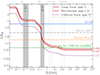 |
Fig. 18. Contribution of new light particles beyond the Standard Model to ΔNeff as a function of their decoupling temperature. Assuming natural units, we report the temperatures in GeV. As a reference we show the contribution of a Goldstone boson (solid brown line), a Weyl fermion (solid red line), and a massless Gauge boson (solid purple line). The grey vertical bands denote the range of temperatures of the QCD phase transition (around 200 MeV) and neutrino decoupling (around 1 MeV), while the thin grey vertical lines mark the annihilation temperature of Standard Model particles. The grey horizontal dot-dashed line represents the current 95% CL limit from Planck TT,TE,EE+lensing+BAO (Planck Collaboration VI 2020). The horizontal dashed lines mark the 95% upper bounds on ΔNeff from Euclid only (in blue) and in combination with current (Planck) and future (CMB-S4+LiteBIRD) CMB surveys (in orange and green, respectively). As explained in Sect. 4.2, we choose to adopt more conservative assumptions regarding the CMB-S4 sensitivity and foreground removal than in a similar figure in the CMB-S4 white paper, Fig. 23 of Abazajian et al. (2016). |
The sensitivity of Euclid to the Hubble parameter will bring strong indications concerning the puzzle raised by the Hubble tension in the near future. We note that the sensitivity of the combination of Euclid spectroscopic and photometric probes is such that, in this case, future CMB observations will not lead to a significant improvement. For instance, in the ΛCDM+∑mν model, the sensitivity will marginally increase from σ(h) = 0.0021 with Euclid +Planck to σ(h) = 0.0016 with Euclid +CMB-S4+LiteBIRD. In the w0waCDM+∑mν model, Euclid data are essential to break the correlation between the dark energy parameters and the other cosmological parameters, including h, therefore, there is no improvement at all in the sensitivity to h due to future CMB experiments (from σ(h) = 0.0036 with Euclid +Planck to σ(h) = 0.0035 with Euclid +CMB-S4+LiteBIRD).
Moreover, Euclid will provide some key information regarding the σ8 tension, having a 1 σ error on S8 = σ8(Ωm/0.3)0.5 of 0.0049 from Euclid only in the ΛCDM+∑mν case. This is an improvement of nearly 3 (2.8) with respect to the DES Y3 3 × 2pt result (Amon et al. 2022; Secco et al. 2022).
Finally, the sensitivity of Euclid to dynamical dark energy parameters, which was already illustrated in previous forecasts assuming a fixed neutrino mass and no extra relativistic species (EC20,Casas et al. 2023), is confirmed in the framework of extended cosmologies with varying ∑mν and ΔNeff. As a matter of fact, the contours derived from Euclid probes do not show significant correlations between the dark energy and neutrino parameters (see Fig. 13). On the other hand, the combination of Euclid with CMB brings back the correlation between ∑mν and {w0, wa}, as we shall comment in the next paragraph on the neutrino mass sensitivity in extended cosmologies.
Neutrino mass sensitivity in extended cosmologies. The constraints on the total neutrino mass from the Euclid primary probes alone are nearly independent of the assumed underlying model, as can be checked in Table 5 and in Fig. 12. However, once combined with external data sets, the constraints become more model dependent.
Floating the number of relativistic relics ΔNeff has a limited impact on ∑mν bounds, but allowing for time-dependent dark energy degrades the mass sensitivity by a significant amount. For instance, the Euclid +Planck sensitivity decreases from σ(∑mν = 60 meV) = 23 meV in the ΛCDM case to 38 meV in the w0waCDM case. Similar trends are observed with the Euclid +CMB-S4+LiteBIRD data set. Previous studies have shown that a correlation between ∑mν and {w0, wa} is already present in the analysis of CMB data alone (Brinckmann et al. 2019). As a matter of fact, the effect of the total neutrino mass and of the dark energy parameters on CMB lensing are difficult to disentangle. The effects of ∑mν (with fixed sound horizon scale, like in the bottom panel of Fig. 1) and of {w0, wa} on the overall amplitude of the matter power spectrum and on the scale of CMB and BAO peaks are also relatively similar, and do not allow us to remove this correlation. Such degeneracies can be removed by including in the analysis additional statistics, such as the bispectrum, as explained in Hahn et al. (2020) (see also Ajani et al. 2020; Chudaykin & Ivanov 2019; Uhlemann et al. 2020). It is nevertheless interesting to see that the constraint on ∑mν never degrades by more than a factor of 2 when the cosmological constant is replaced by dynamical dark energy.
When the dark energy and radiation density parameters {w0, wa, ΔNeff} are varied simultaneously, the sensitivity remains close to that in the w0waCDM+∑mν model. In the w0waCDM+∑mν+ΔNeff model, it is still possible to get about 2 σ evidence for a non-zero mass from the Euclid +CMB-S4+LiteBIRD combination.
8. Conclusions
Building on the work of Euclid Collaboration (2024a), we have implemented and validated a pipeline to consistently forecast the constraints on the neutrino parameters (such as mass and abundance) that will be measurable from the upcoming Euclid mission of the European Space Agency. We have studied how to model the observables of the photometric survey (allowing for cosmic shear and galaxy clustering measurements) and those of the spectroscopic survey (allowing for a reconstruction of the galaxy clustering power spectrum) for cosmologies including massive neutrinos, additional relativistic degrees of freedom, and variations in the dark energy equation of state.
We find that the Fisher matrices computed with the CosmicFish and MontePython pipelines agree to a 10% level even after marginalising over all corresponding nuisance parameters, independently of which EBS (CAMB or CLASS) is used. For the purposes of this implementation, we have also compared various nonlinear treatments. We conclude that for our purpose the predictions of HMcode (Mead et al. 2021) are the closest to numerical simulations for the cosmological models considered here, even outperforming some of the emulators that we have considered.
The validated forecast pipeline predicts a great deal of complementarity between the various probes measured by Euclid, particularly between the photometric and spectroscopic surveys. The combination of these probes will help to break the degeneracies between the parameters {H0, σ8, ΔNeff, ∑mν, w0, wa}. There is a strong complementarity with additional probes as well, which can be used to lift the residual degeneracy among the small-scale fluctuation amplitude, Hubble constant, and the neutrino parameters. Once combined with data from CMB anisotropy experiments, the Euclid data will lead to extremely tight constraints on {σ8, H0, ∑mν, Neff}.
Indeed, we find that while Euclid data alone will already allow us to constrain σ(∑mν = 60 meV) = 53 meV in the standard ΛCDM+∑mν model, its combination with CMB anisotropy data from Planck will lead to a sensitivity of σ(∑mν = 60 meV) = 23 meV. Thus, we can expect Euclid +Planck data to raise evidence for a non-zero neutrino mass at least at the 2.6 σ level. If the combined data turns out to be best fit with ∑mν ≃ 60 meV, it would indicate a preference for normal ordering over inverted ordering roughly at the 2 σ level. In combination with future CMB data from LiteBIRD and CMB Stage-IV, Euclid will reach a sensitivity of around σ(∑mν = 60 meV) = 16 meV, which will allow for a neutrino mass detection at almost 4 σ. Under the same assumption, we would obtain a clear disambiguation of the neutrino mass hierarchy at 2.5 σ. These constraints are only mildly sensitive to the addition of ultra-relativistic degrees of freedom (ΔNeff > 0) and end up being degrading only by a factor of roughly 2 when considering a flexible model of time-varying dark energy.
Euclid is also expected to measure the Hubble parameter with exquisite precision in these cosmologies, with an uncertainty expected to reach 0.1–0.3 km s−1 Mpc−1 in combination with CMB data. This will bring very strong clues regarding the puzzle raised by the current Hubble tension.
The determination of the effective neutrino number Neff by CMB experiments is limited by a parameter degeneracy between Neff and H0. The Euclid probes alone will be sensitive to Neff and, even more importantly, when combined with CMB data, they will be able to partially lift this degeneracy. Assuming a fiducial model with no additional relativistic degrees of freedom beyond standard neutrinos (Neff = 3.044), the combination of Planck data and Euclid primary probes will provide a 95% CL upper bound ΔNeff < 0.144 in the ΛCDM+∑mν+Neff case. The bound will be further tightened to ΔNeff < 0.063 with future CMB data from LiteBIRD and CMB Stage-IV. These predictions remain stable when marginalising over dynamical dark energy parameters. Such bounds will constrain many well-motivated models of additional relativistic particles such as Goldstone bosons, Weyl fermions, or massless gauge bosons. Not only will decoupling times after the QCD transition be potentially ruled out by Euclid alone, but in combination with CMB experiments, decoupling times even slightly before the QCD transition can be constrained. Indeed, in combination with future CMB surveys, Euclid will come close to excluding the presence of these particles at any decoupling temperature (even far before the QCD transition, see Fig. 18).
In summary, Euclid will put tight constraints on the parameters of the ΛCDM model as well as some of its most commonly considered extensions, while bringing strong indications concerning the Hubble constant tension. In combination with either current or future CMB data, Euclid will constrain neutrino physics, potentially providing the first detection of a non-zero neutrino mass, along with some strong hints about the mass ordering. Moreover, the combined data will have an enhanced sensitivity to the effective number of neutrinos and a significant potential to rule out many candidates for light relics beyond the Standard Model. As such, Euclid will consolidate the ability of precision cosmology to probe neutrino physics.
We note that, if neutrinos are Majorana particles, their mass can also be constrained by means of neutrinoless double-β-decay experiments (Cirigliano et al. 2022); however, there is no evidence for lepton number violation yet.
However, the effect of the ordering is slightly enhanced by the nonlinear evolution (Wagner et al. 2012) and the detection might become possible in the future, especially with upcoming line-intensity mapping surveys, as suggested in Pritchard & Pierpaoli (2008) and Bernal et al. (2021).
During the completion of this work, there is a claim that this value shall be revised to Neff = 3.043 following a high-precision calculation of QED effects during electron-positron annihilation (Cielo et al. 2023). In this work we stick to Neff = 3.044 – this difference has no impact on our sensitivity forecasts.
In Eq. (4), H(z) has units of km s−1 Mpc−1, c of km s−1, r of Mpc,  of Mpc3, and WiX(z) of Mpc−1, while all other quantities are dimensionless.
For a more general model of intrinsic alignment see for example Ref. Chen et al. (2024).
Here, we use the same sky fraction, as well as other specifications, of EC20, however, some of them have changed since then (see, for instance, the reduction of wide survey area from 15 000 deg2 to 14 000 deg2 reported in Ref. Euclid Collaboration 2022), and keep changing continuously based on the performance of the satellite.
In this context, it is not obvious whether one should use Pcc or Pmm. A comparison with simulations suggests, however, that using Pcc is a better approximation, see Eq. (8) of Villaescusa-Navarro et al. (2018) or the discussion that follows Eq. (6.13) of Castorina et al. (2015).
Contrary to the recipe for photometric observables, the recipe for spectroscopic observables is built on the linear power spectrum, and the nonlinear effects are modelled through the Lorentzian factor and the damping of the wiggle-only power spectrum to which a de-wiggled contribution is added to restore the broadband shape of the power spectrum; the nonlinear corrections of Sect. 3.3 are never applied here.
To compute the second derivatives using a finite difference scheme, after computing the likelihood at the best fit, the code needs to perform two likelihood evaluations for each of the N second derivatives with α = β, and four evaluations for each of the N(N − 1)/2 cross-derivatives with α ≠ β, leading to a total of 2N2 evaluations.
These pipelines correspond to those called ‘CosmicFish internal’ in Euclid Collaboration (2024a), denoted as CF/int/CAMB and CF/int/CLASS. In this paper, we omit the ‘int’ since we do not use external precomputed spectra.
We note that the effects of ∑mν and ΔNeff on the BAO peaks are intrinsically different. Indeed a variation in the number of relativistic species leads to an irreducible phase-shift of the BAO peaks due to the gravitational boost of CDM perturbations at horizon entry sourced by the anisotropic stress of free-streaming species. On the other hand, a variation in ∑mν changes the distance of the BAO peaks by means of background effects, which can be also compensated by a variation in another cosmological parameter (such as h and Ωc, 0).
The CAMB file fortran/halofit.f90 contains a function THalofit_GetNonLinRatios() that computes a characteristic radius rmid with a bisection method. The bisection accuracy is set by the line: if (abs(diff).le.0.001) then ... It is essential to substitute 0.001 with a smaller tolerance equal to (or smaller than) 10−6, otherwise, the error on rmid is way too large given the Euclid sensitivity, and leads to inaccurate derivatives in the Fisher matrix calculation. In this work we use a tolerance of 10−6.
Acknowledgments
The Euclid Consortium acknowledges the European Space Agency and a number of agencies and institutes that have supported the development of Euclid, in particular the Agenzia Spaziale Italiana, the Austrian Forschungsförderungsgesellschaft funded through BMK, the Belgian Science Policy, the Canadian Euclid Consortium, the Deutsches Zentrum für Luft-und Raumfahrt, the DTU Space and the Niels Bohr Institute in Denmark, the French Centre National d’Etudes Spatiales, the Fundação para a Ciência e a Tecnologia, the Hungarian Academy of Sciences, the Ministerio de Ciencia, Innovación y Universidades, the National Aeronautics and Space Administration, the National Astronomical Observatory of Japan, the Netherlandse Onderzoekschool Voor Astronomie, the Norwegian Space Agency, the Research Council of Finland, the Romanian Space Agency, the State Secretariat for Education, Research, and Innovation (SERI) at the Swiss Space Office (SSO), and the United Kingdom Space Agency. A complete and detailed list is available on the Euclid web site (https://www.euclid-ec.org). We warmly thank Julien Bel for providing matter power spectra measurements from the DEMNUni simulations. N.F. is supported by the Italian Ministry of University and Research (MUR) through Rita Levi Montalcini project “Tests of gravity at cosmological scales” with reference PGR19ILFGP. N.F. and F.P. also acknowledge the FCT project with ref. number PTDC/FIS-AST/0054/2021. F.P. acknowledges partial support from the INFN grant InDark and the Departments of Excellence grant L.232/2016 of the Italian Ministry of University and Research (MUR). S.P.’s simulations were performed with computing resources granted by RWTH Aachen University under project thes1329. Z.S. acknowledges funding from DFG project 456622116 and support from the IRAP and IN2P3 Lyon computing centers. N.S. acknowledges support from the Maria de Maetzu fellowship grant: CEX2019-000918-M, financiado por MCIN/AEI/10.13039/501100011033. The DEMNUni simulations were carried out in the framework of “The Dark Energy and Massive-Neutrino Universe” project, using the Tier-0 IBM BG/Q Fermi machine and the Tier-0 Intel OmniPath Cluster Marconi-A1 of the Centro Interuniversitario del Nord-Est per il Calcolo Elettronico (CINECA). We acknowledge a generous CPU and storage allocation by the Italian Super-Computing Resource Allocation (ISCRA) as well as from the coordination of the “Accordo Quadro MoU per lo svolgimento di attività congiunta di ricerca Nuove frontiere in Astrofisica: HPC e Data Exploration di nuova generazione”, together with storage from INFN-CNAF and INAF-IA2.
References
- Abazajian, K. N., Adshead, P., Ahmed, Z., et al. 2016, arXiv e-prints [arXiv:1610.02743] [Google Scholar]
- Adamek, J., Angulo, R. E., Arnold, C., et al. 2023, JCAP, 06, 035 [NASA ADS] [Google Scholar]
- Ajani, V., Peel, A., Pettorino, V., et al. 2020, Phys. Rev. D, 102, 103531 [Google Scholar]
- Aker, M., Batzler, D., Beglarian, A., et al. 2024, arXiv e-prints [arXiv:2406.13516] [Google Scholar]
- Akita, K., & Yamaguchi, M. 2020, JCAP, 08, 012 [CrossRef] [Google Scholar]
- Alam, S., Aubert, M., Avila, S., et al. 2021, Phys. Rev. D, 103, 083533 [NASA ADS] [CrossRef] [Google Scholar]
- Alcock, C., & Paczynski, B. 1979, Nature, 281, 358 [NASA ADS] [CrossRef] [Google Scholar]
- Allen, S. W., Evrard, A. E., & Mantz, A. B. 2011, ARA&A, 49, 409 [Google Scholar]
- Allison, R., Caucal, P., Calabrese, E., Dunkley, J., & Louis, T. 2015, Phys. Rev. D, 92, 123535 [NASA ADS] [CrossRef] [Google Scholar]
- Allys, E., Arnold, K., Aumont, J., et al. 2023, PTEP, 2023, 042F01 [Google Scholar]
- Amon, A., Gruen, D., Troxel, M. A., et al. 2022, Phys. Rev. D, 105, 023514 [NASA ADS] [CrossRef] [Google Scholar]
- Angulo, R. E., Zennaro, M., Contreras, S., et al. 2021, MNRAS, 507, 5869 [NASA ADS] [CrossRef] [Google Scholar]
- Archidiacono, M., & Gariazzo, S. 2022, Universe, 8, 175 [NASA ADS] [CrossRef] [Google Scholar]
- Archidiacono, M., Brinckmann, T., Lesgourgues, J., & Poulin, V. 2017, JCAP, 02, 052 [CrossRef] [Google Scholar]
- Archidiacono, M., Hannestad, S., & Lesgourgues, J. 2020, JCAP, 09, 021 [CrossRef] [Google Scholar]
- Audren, B., Lesgourgues, J., Bird, S., Haehnelt, M. G., & Viel, M. 2013, JCAP, 01, 026 [CrossRef] [Google Scholar]
- Bahcall, N. A., & Fan, X.-H. 1998, ApJ, 504, 1 [NASA ADS] [CrossRef] [Google Scholar]
- Bashinsky, S., & Seljak, U. 2004, Phys. Rev. D, 69, 083002 [CrossRef] [Google Scholar]
- Basse, T., Bjaelde, O. E., Hamann, J., Hannestad, S., & Wong, Y. Y. Y. 2014, JCAP, 05, 021 [CrossRef] [Google Scholar]
- Baumann, D., Beutler, F., Flauger, R., et al. 2019, Nat. Phys., 15, 465 [NASA ADS] [CrossRef] [Google Scholar]
- Bennett, J. J., Buldgen, G., De Salas, P. F., et al. 2021, JCAP, 04, 073 [CrossRef] [Google Scholar]
- Bernal, J. L., Caputo, A., Villaescusa-Navarro, F., & Kamionkowski, M. 2021, Phys. Rev. Lett., 127, 131102 [Google Scholar]
- Bird, S., Viel, M., & Haehnelt, M. G. 2012, MNRAS, 420, 2551 [Google Scholar]
- Blas, D., Lesgourgues, J., & Tram, T. 2011, JCAP, 07, 034 [CrossRef] [Google Scholar]
- Bocquet, S., Dietrich, J. P., Schrabback, T., et al. 2019, ApJ, 878, 55 [Google Scholar]
- Bonamente, M. 2020, J. Appl. Stat., 47, 2044 [NASA ADS] [CrossRef] [Google Scholar]
- Bond, J. R., Efstathiou, G., & Silk, J. 1980, Phys. Rev. Lett., 45, 1980 [NASA ADS] [CrossRef] [Google Scholar]
- Boyle, A., & Komatsu, E. 2018, JCAP, 03, 035 [CrossRef] [Google Scholar]
- Brinckmann, T., Hooper, D. C., Archidiacono, M., Lesgourgues, J., & Sprenger, T. 2019, JCAP, 01, 059 [CrossRef] [Google Scholar]
- Carbone, C., Fedeli, C., Moscardini, L., & Cimatti, A. 2012, JCAP, 03, 023 [CrossRef] [Google Scholar]
- Carbone, C., Petkova, M., & Dolag, K. 2016, JCAP, 07, 034 [CrossRef] [Google Scholar]
- Cash, W. 1979, ApJ, 228, 939 [Google Scholar]
- Castorina, E., Sefusatti, E., Sheth, R. K., Villaescusa-Navarro, F., & Viel, M. 2014, JCAP, 02, 049 [CrossRef] [Google Scholar]
- Castorina, E., Carbone, C., Bel, J., Sefusatti, E., & Dolag, K. 2015, JCAP, 07, 043 [CrossRef] [Google Scholar]
- Cerbolini, M. C. A., Sartoris, B., Xia, J.-Q., et al. 2013, JCAP, 06, 020 [CrossRef] [Google Scholar]
- Chen, S.-F., Vlah, Z., & White, M. 2022, JCAP, 02, 008 [NASA ADS] [CrossRef] [Google Scholar]
- Chen, S., DeRose, J., Zhou, R., et al. 2024, arXiv e-prints [arXiv:2407.04795] [Google Scholar]
- Chevallier, M., & Polarski, D. 2001, Int. J. Mod. Phys. D, 10, 213 [Google Scholar]
- Chudaykin, A., & Ivanov, M. M. 2019, JCAP, 11, 034 [CrossRef] [Google Scholar]
- Chudaykin, A., Ivanov, M. M., & Simonović, M. 2021, Phys. Rev. D, 103, 043525 [CrossRef] [Google Scholar]
- Cielo, M., Escudero, M., Mangano, G., & Pisanti, O. 2023, Phys. Rev. D, 108, L121301 [CrossRef] [Google Scholar]
- Cirigliano, V., Davoudi, Z., Dekens, W., et al. 2022, arXiv e-prints [arXiv:2203.12169] [Google Scholar]
- Costanzi, M., Villaescusa-Navarro, F., Viel, M., et al. 2013, JCAP, 12, 012 [Google Scholar]
- Costanzi, M., Saro, A., Bocquet, S., et al. 2021, Phys. Rev. D, 103, 043522 [Google Scholar]
- D’Amico, G., Gleyzes, J., Kokron, N., et al. 2020, JCAP, 05, 005 [Google Scholar]
- Dasgupta, B., & Kopp, J. 2021, Phys. Rept., 928, 1 [CrossRef] [Google Scholar]
- Di Luzio, L., Giannotti, M., Nardi, E., & Visinelli, L. 2020, Phys. Rept., 870, 1 [NASA ADS] [Google Scholar]
- di Valentino, E., Gariazzo, S., & Mena, O. 2022, Phys. Rev. D, 106, 043540 [CrossRef] [Google Scholar]
- Drewes, M., Georis, Y., Klasen, M., Wiggering, L. P., & Wong, Y. Y. Y. 2024, JCAP, 06, 032 [CrossRef] [Google Scholar]
- Dvorkin, C., Meyers, J., Adshead, P., et al. 2022, arXiv e-prints [arXiv:2203.07943] [Google Scholar]
- Esteban, I., Gonzalez-Garcia, M. C., Maltoni, M., Schwetz, T., & Zhou, A. 2020, JHEP, 09, 178 [CrossRef] [Google Scholar]
- Euclid Collaboration (Blanchard, A., et al.) 2020, A&A, 642, A191 [NASA ADS] [CrossRef] [EDP Sciences] [Google Scholar]
- Euclid Collaboration (Knabenhans, M., et al.) 2021a, MNRAS, 505, 2840 [NASA ADS] [CrossRef] [Google Scholar]
- Euclid Collaboration (Martinelli, M., et al.) 2021b, A&A, 649, A100 [NASA ADS] [CrossRef] [EDP Sciences] [Google Scholar]
- Euclid Collaboration (Scaramella, R., et al.) 2022, A&A, 662, A112 [NASA ADS] [CrossRef] [EDP Sciences] [Google Scholar]
- Euclid Collaboration (Castro, T., et al.) 2023, A&A, 671, A100 [CrossRef] [EDP Sciences] [Google Scholar]
- Euclid Collaboration (Casas, S., et al.) 2024a, A&A, 682, A90 [NASA ADS] [CrossRef] [EDP Sciences] [Google Scholar]
- Euclid Collaboration (Cropper, M., et al.) 2024b, A&A, in press, https://doi.org/10.1051/0004-6361/202450996 [Google Scholar]
- Euclid Collaboration (Jahnke, K., et al.) 2024c, A&A, in press, https://doi.org/10.1051/0004-6361/202450786 [Google Scholar]
- Euclid Collaboration (Mellier, Y., et al.) 2024d, A&A, in press, https://doi.org/10.1051/0004-6361/202450810 [Google Scholar]
- Froustey, J. 2022, Ph.D. Thesis, Institut d’Astrophysique de Paris, France, Paris, France [Google Scholar]
- Froustey, J., Pitrou, C., & Volpe, M. C. 2020, JCAP, 12, 015 [CrossRef] [Google Scholar]
- Giri, S. K., & Schneider, A. 2021, JCAP, 12, 046 [CrossRef] [Google Scholar]
- Gonzalez-Garcia, M., & Yokoyama, M. 2022, PTEP, 2022, 083C01 [Google Scholar]
- Hadzhiyska, B., Wolz, K., Azzoni, S., et al. 2023, Open J. Astrophys., 6, 23 [NASA ADS] [Google Scholar]
- Hahn, C., Villaescusa-Navarro, F., Castorina, E., & Scoccimarro, R. 2020, JCAP, 03, 040 [CrossRef] [Google Scholar]
- Hannestad, S. 2006, Ann. Rev. Nucl. Part. Sci., 56, 137 [NASA ADS] [CrossRef] [Google Scholar]
- Holder, G., Haiman, Z., & Mohr, J. 2001, ApJL, 560, L111 [NASA ADS] [CrossRef] [Google Scholar]
- Hou, Z., Keisler, R., Knox, L., Millea, M., & Reichardt, C. 2013, Phys. Rev. D, 87, 083008 [NASA ADS] [CrossRef] [Google Scholar]
- Hu, W., Scott, D., Sugiyama, N., & White, M. J. 1995, Phys. Rev. D, 52, 5498 [Google Scholar]
- Hu, W., Eisenstein, D. J., & Tegmark, M. 1998, Phys. Rev. Lett., 80, 5255 [NASA ADS] [CrossRef] [Google Scholar]
- Ivanov, M. M., Simonović, M., & Zaldarriaga, M. 2020a, Phys. Rev. D, 101, 083504 [NASA ADS] [CrossRef] [Google Scholar]
- Ivanov, M. M., Simonović, M., & Zaldarriaga, M. 2020b, JCAP, 05, 042 [CrossRef] [Google Scholar]
- Kaiser, N. 1987, MNRAS, 227, 1 [Google Scholar]
- Kawasaki, M., & Nakayama, K. 2013, Ann. Rev. Nucl. Part. Sci., 63, 69 [NASA ADS] [CrossRef] [Google Scholar]
- Kilbinger, M., Heymans, C., Asgari, M., et al. 2017, MNRAS, 472, 2126 [Google Scholar]
- Kirby, M., Rozo, E., Morris, R. G., et al. 2019, arXiv e-prints [arXiv:1910.13548] [Google Scholar]
- Kravtsov, A., & Borgani, S. 2012, ARA&A, 50, 353 [NASA ADS] [CrossRef] [Google Scholar]
- Lambiase, G., Mohanty, S., Narang, A., & Parashari, P. 2019, Eur. Phys. J. C, 79, 141 [NASA ADS] [CrossRef] [Google Scholar]
- Lattanzi, M., & Gerbino, M. 2018, Front. Phys., 5, 70 [Google Scholar]
- Lesci, G. F., Marulli, F., Moscardini, L., et al. 2022, A&A, 659, A88 [NASA ADS] [CrossRef] [EDP Sciences] [Google Scholar]
- Lesgourgues, J., & Pastor, S. 2006, Phys. Rept., 429, 307 [NASA ADS] [CrossRef] [Google Scholar]
- Lesgourgues, J., & Pastor, S. 2012, Adv. High Energy Phys., 2012, 608515 [CrossRef] [Google Scholar]
- Lesgourgues, J., & Tram, T. 2011, JCAP, 09, 032 [CrossRef] [Google Scholar]
- Lesgourgues, J., & Verde, L. 2022, PTEP, 2022, 083C01 [Google Scholar]
- Lesgourgues, J., Pastor, S., & Perotto, L. 2004, Phys. Rev. D, 70, 045016 [Google Scholar]
- Lesgourgues, J., Mangano, G., Miele, G., & Pastor, S. 2013, Neutrino Cosmology (Cambridge University Press) [CrossRef] [Google Scholar]
- Linder, E. V. 2003, Phys. Rev. Lett., 90, 091301 [Google Scholar]
- Mangano, G., Miele, G., Pastor, S., & Peloso, M. 2002, Phys. Lett. B, 534, 8 [CrossRef] [Google Scholar]
- Mangano, G., Miele, G., Pastor, S., et al. 2005, Nucl. Phys. B, 729, 221 [Google Scholar]
- Mantz, A., Allen, S. W., Ebeling, H., & Rapetti, D. 2008, MNRAS, 387, 1179 [CrossRef] [Google Scholar]
- Marsh, D. J. E. 2016, Phys. Rept., 643, 1 [NASA ADS] [CrossRef] [Google Scholar]
- Mead, A. J., Brieden, S., Tröster, T., & Heymans, C. 2021, MNRAS, 502, 1401 [Google Scholar]
- Mele, S. 2015, Adv. Ser. Direct. High Energy Phys., 23, 89 [CrossRef] [Google Scholar]
- Mohr, J. J. 2005, ASP Conf. Ser., 339, 140 [NASA ADS] [Google Scholar]
- Oukbir, J., & Blanchard, A. 1997, A&A, 317, 1 [NASA ADS] [Google Scholar]
- Palanque-Delabrouille, N., Yèche, C., Schöneberg, N., et al. 2020, JCAP, 04, 038 [Google Scholar]
- Parimbelli, G., Viel, M., & Sefusatti, E. 2019, JCAP, 01, 010 [CrossRef] [Google Scholar]
- Parimbelli, G., Carbone, C., Bel, J., et al. 2022, JCAP, 11, 041 [Google Scholar]
- Park, H., Shapiro, P. R., Komatsu, E., et al. 2013, ApJ, 769, 93 [Google Scholar]
- Planck Collaboration VI. 2020, A&A, 641, A6, [Erratum: A&A 652, C4 (2021)] [NASA ADS] [CrossRef] [EDP Sciences] [Google Scholar]
- Pritchard, J. R., & Pierpaoli, E. 2008, Phys. Rev. D, 78, 065009 [NASA ADS] [CrossRef] [Google Scholar]
- Project 8 Collaboration (Ashtari Esfahani, A., et al.) 2022, arXiv e-prints [arXiv:2203.07349] [Google Scholar]
- Reiprich, T. H., & Boehringer, H. 2002, ApJ, 567, 716 [NASA ADS] [CrossRef] [Google Scholar]
- Rossi, G., Yèche, C., Palanque-Delabrouille, N., & Lesgourgues, J. 2015, Phys. Rev. D, 92, 063505 [NASA ADS] [CrossRef] [Google Scholar]
- Sailer, N., Chen, S.-F., & White, M. 2022, JCAP, 10, 007 [CrossRef] [Google Scholar]
- Sakr, Z., Ilic, S., & Blanchard, A. 2022, A&A, 666, A34 [NASA ADS] [CrossRef] [EDP Sciences] [Google Scholar]
- Sartoris, B., Biviano, A., Fedeli, C., et al. 2016, MNRAS, 459, 1764 [Google Scholar]
- Schmittfull, M., Simonović, M., Ivanov, M. M., Philcox, O. H. E., & Zaldarriaga, M. 2021, JCAP, 05, 059 [CrossRef] [Google Scholar]
- Schneider, A., Stoira, N., Refregier, A., et al. 2020a, JCAP, 04, 019 [CrossRef] [Google Scholar]
- Schneider, A., Refregier, A., Grandis, S., et al. 2020b, JCAP, 04, 020 [Google Scholar]
- Secco, L. F., Samuroff, S., Krause, E., et al. 2022, Phys. Rev. D, 105, 023515 [NASA ADS] [CrossRef] [Google Scholar]
- Semboloni, E., Hoekstra, H., Schaye, J., van Daalen, M. P., & McCarthy, I. J. 2011, MNRAS, 417, 2020 [Google Scholar]
- Senatore, L., & Zaldarriaga, M. 2017, arXiv e-prints [arXiv:1707.04698] [Google Scholar]
- Sprenger, T., Archidiacono, M., Brinckmann, T., Clesse, S., & Lesgourgues, J. 2019, JCAP, 02, 047 [Google Scholar]
- Spurio Mancini, A., & Bose, B. 2023, Open J. Astrophys., 6, 40 [NASA ADS] [Google Scholar]
- Takahashi, R., Sato, M., Nishimichi, T., Taruya, A., & Oguri, M. 2012, ApJ, 761, 152 [Google Scholar]
- Uhlemann, C., Friedrich, O., Villaescusa-Navarro, F., Banerjee, A., & Codis, S. 2020, MNRAS, 495, 4006 [NASA ADS] [CrossRef] [Google Scholar]
- Vagnozzi, S., Brinckmann, T., Archidiacono, M., et al. 2018, JCAP, 09, 001 [NASA ADS] [Google Scholar]
- Vikhlinin, A., Kravtsov, A. V., Burenin, R. A., et al. 2009, ApJ, 692, 1060 [Google Scholar]
- Villaescusa-Navarro, F., Banerjee, A., Dalal, N., et al. 2018, ApJ, 861, 53 [NASA ADS] [CrossRef] [Google Scholar]
- Wagner, C., Verde, L., & Jimenez, R. 2012, ApJL, 752, L31 [NASA ADS] [CrossRef] [Google Scholar]
- Wang, Y., Chuang, C.-H., & Hirata, C. M. 2013, MNRAS, 430, 2446 [NASA ADS] [CrossRef] [Google Scholar]
- Weinberg, N. N., & Kamionkowski, M. 2003, MNRAS, 341, 251 [NASA ADS] [CrossRef] [Google Scholar]
- White, S. D. M., Navarro, J. F., Evrard, A. E., & Frenk, C. S. 1993, Nature, 366, 429 [Google Scholar]
- Yankelevich, V., & Porciani, C. 2019, MNRAS, 483, 2078 [NASA ADS] [CrossRef] [Google Scholar]
Appendix A: Effect of the numerical derivative method
In this work, we set CosmicFish to compute the derivative of observables with respect to cosmological parameters using double-sided derivatives, also called 3-point derivatives (3PT). To check whether our results are stable against the computation of numerical derivatives, we performed a test using a four-point forward stencil method (4PT_FWD). We compare the unmarginalised and marginalised errors inferred from the two methods in Fig. A.1. We see that the impact on unmarginalised errors are below 0.1%, while the marginalised errors are within 0.4% of each other, that is, well below our validation threshold. We have also checked in 2D contours that the directions of correlation are preserved. Noticeably, the errors from the 4PT_FWD method are always below the errors from 3PT, showing that our default choice is actually conservative. We conclude that our results are robust against the numerical derivative method.
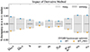 |
Fig. A.1. Effect on the marginalised and unmarginalised errors of changing the numerical derivative method from 3PT to 4PT_FWD in the CF/CAMB pipeline. Here we choose the case of the spectroscopic probe with optimistic settings, and we stick to the same assumptions and precision parameters as in the rest of the validation (Sect. 6). In this test, the nuisance parameters are kept fixed for simplicity. The marginalisation takes place over other cosmological parameters. |
Appendix B: Settings and accuracy of Einstein–Boltzmann solvers
The question of the accuracy settings required by Euclid forecasts in the CAMB and CLASS EBSs has been discussed in depth in Sect. 6 and Appendix A of Euclid Collaboration (2024a). Here we focus on new aspects related to the promotion of ∑mν and Neff as varied parameters. We refer the reader to Euclid Collaboration (2024a) for more details on other aspects.
Default accuracy settings in the public CAMB and CLASS versions have been established in order to ensure unbiased MCMC parameter inference from current CMB and large-scale structure surveys. As a general trend, the estimation of Bayesian credible intervals requires less accurate theory predictions when running MCMC than when computing Fisher matrices. Indeed, it is well-known that the excursion in parameter space performed by MCMC tends to smooth out the effect of random numerical noise (in observables and likelihoods) on the estimation of parameter credible intervals. Instead, in Fisher forecasts, the calculation of numerical derivatives with very small step sizes and the inversion of Fisher matrices into covariance matrices tend to enhance the sensitivity of unmarginalised and marginalised errors to such numerical noise.
For that reason, like in Euclid Collaboration (2024a), we use enhanced accuracy settings in Fisher forecasts, using the agreement between marginalised error bars inferred from the CAMB and CLASS pipelines as an estimator of convergence. When running the MP/MCMC pipeline, we instead stick to CLASS default precision. The fact that our CF/CAMB and CF/CLASS forecasts agree so well (see Figs. 6 to 8) and remain stable against small changes in the choice of derivative step sizes (see Appendix C) proves that our high accuracy settings are sufficient to maintain numerical noise below the Euclid sensitivity level. Finally, the fact that our Fisher ellipses agree so well with our MCMC 2D contours whenever the posterior is Gaussian with respect to pairs of parameters (see Figs. 9 to 11) proves that default precision is sufficient for the purpose of fitting Euclid data with MCMC.
To be precise, this test proves that our accuracy settings are sufficient to keep random numerical noise (which is by construction independent in CAMB and CLASS ) at a sufficiently low level. It does not prove that the modelling of physical effects is accurate enough, since both codes could in principle rely on the same incorrect modelling of some physical mechanism, and compute observables with the same systematic error. A potential example of this, related to the modelling of massive neutrinos, is discussed in Appendix B.1. The only way to mitigate this risk is to compare the results of fits performed with modified versions of EBSs relying on several different schemes for the treatment of hydrogen recombination, of the neutrino phase-space distribution, of the truncation of the Boltzmann hierarchy, of gauge freedom, etc. This goes beyond the level of this work. Note however that such tests have been done repeatedly in many theoretical papers and within several observational collaborations, while the modelling of the w0waCDM+∑mν+Neff model has been intensely scrutinised over three decades. Thus, the impact of these different schemes is well-known and the implementation of w0waCDM+∑mν+Neff in CAMB and CLASS can be considered as robust. If CAMB and CLASS did compute observables with the same systematic error, it would be due to a new and yet unidentified physical ingredient, rather than a wrong numerical modelling of the physical assumptions currently going into this cosmological scenario.
B.1. Cosmological parameters
In this work, we use CAMB version 1.3.7. When using the photometric likelihood, we set halofit_version = 9 to compute nonlinear corrections with the latest version of HMcode (Mead et al. 2021). For CLASS, we use a branch forked from v3.2 that implements the same version of HMcode. This branch will soon be released publicly as v3.3. In the photometric case, we activate accurate HMcode calculations with non linear = hmcode2020.
The parameters passed to CAMB and CLASS to account for our fiducial cosmology are the same as described in Appendix A.1 of Euclid Collaboration (2024a) up to small shifts in the fiducial values. These shifts aim at matching the Planck best-fit values and the updated prediction Neff = 3.044 of the standard neutrino-decoupling model (Froustey et al. 2020; Bennett et al. 2021). They have no impact whatsoever on our results for predicted errors.
We note that σ8 is not implemented as a possible input parameter in CAMB. We circumvent this issue within CosmicFish by calling CAMB twice, the first time with an arbitrary primordial amplitude parameter As, and the second time with the exact value of As needed to obtain the desired σ8. In the CLASS case, σ8 is passed as a input parameter and the same steps are performed internally.
There are non-trivial aspects related to the setting of neutrino parameters. The approach of CAMB and CLASS are quite different as far as massive neutrinos are concerned. As a matter of fact, a very precise treatment of the neutrino sector matching the predictions of the standard neutrino decoupling model, described for instance in Froustey et al. (2020) and in Bennett et al. (2021), would have to take into account flavor-dependent non-thermal distortions and flavor mixing in each mass eigenstate. For the sake of computational speed and simplicity, CAMB and CLASS use by default some effective approaches that attempt to mimic these effects while sticking to a single Fermi–Dirac phase-space distribution shared by all massive neutrinos. There are several ways to set up such an effective description. CAMB and CLASS use different ones, each with its own motivation.
These two different treatments generate sub-percent-level differences in the final matter power spectrum, which are too small to be relevant in the analysis of real Euclid data. However, for the purpose of Fisher matrix calculations, these tiny differences can be amplified by the calculation of numerical derivatives. Thus, for the purpose of validating our Fisher pipelines against each other, we stick to a precise mapping between CAMB and CLASS parameters, which ensures that the latter code sticks to the same assumptions as the former. This mapping is very similar to the one used in Euclid Collaboration (2024a) but allows for arbitrary values of ∑mν and Neff.
In our Fisher forecasts, we call CAMB with num_nu_massive set to 1, num_nu_massless set to the varied parameter Neff minus 1, and a neutrino mass set to the varied parameter ∑mν. Note that the forecast pipeline varies Neff in a range given by the fiducial value 3.044 plus or minus one per cent, such that 3.01 < Neff < 3.08. CAMB uses by default a neutrino model corresponding to its internal option share_delta_neff = T.22 This option triggers several non-trivial operations. Given our input, CAMB always assumes two massless and one massive neutrino species, and rescales their respective temperature to a common value such that the total neutrino density in the early universe matches Neff. For that purpose, the true effective number of ultra-relativistic degrees of freedom (for instance massless neutrinos) actually used in the CAMB equations is redefined internally from (Neff − 1) to a new number:
![$$ \begin{aligned} N_\mathrm{ur} = 2 + \frac{2}{3} \Big (N_{\rm eff} - \mathrm{floor} [N_{\rm eff}]\Big )\, , \end{aligned} $$](/articles/aa/full_html/2025/01/aa50859-24/aa50859-24-eq59.gif)
where floor[Neff] denotes the largest integer smaller than Neff. Massive neutrinos are modelled as a perfect Fermi–Dirac species with a temperature Tν and fractional density Ων computed as
We note that, for the sake of consistency, the last equation uses on purpose the numerical value of the ratio ∑mν/[Ων, 0h2] computed in the instantaneous decoupling limit, 94.07 eV, and not the more realistic value 93.12 eV (Froustey 2022). To mimic exactly the same settings in CLASS, we fix N_ncdm to 1, and we set the three input parameters (N_ur, T_ncdm, Omega_ncdm) to the three number calculated respectively with Eqs. (B.1) to (B.3).
As explained in Sect. 2.2, the final MCMC forecasts of Sect. 7 assume instead three massive neutrinos (degenerate in mass and such that each of the three species contributes to Neff as 3.044/3) plus extra relativistic species contributing as (Neff − 3.044). We achieve this by setting N_ncdm to 1, deg_ncdm to 3, and the parameters (N_ur, T_ncdm, Omega_ncdm) to:
B.2. Accuracy parameters
Euclid Collaboration (2024a) have defined some enhanced accuracy settings for the CAMB and CLASS codes such that, in the framework of the w0waCDM model, Euclid Fisher forecasts performed with either code are stable and in good agreement with each other. Euclid Collaboration (2024a) also explained that in the case of CAMB, on top of increasing some accuracy parameters, it is necessary to adapt the code in order to increase the precision of a bisection algorithm used by both HALOFIT and HMcode.23 This adaptation is still relevant in our context and we use it throughout our validation process.
From the point of view of accuracy setting, the difference between Euclid Collaboration (2024a) and this work is that we now need to compute some derivatives with respect to the parameters ∑mν and Neff. We found that derivatives with respect to Neff are stable and accurate enough with the settings used in Euclid Collaboration (2024a). Instead, getting accurate derivatives with respect to ∑mν requires particular care. Even after solving the issue of the potentially different modelling of massive neutrinos in the way discussed in the previous subsection, one is confronted with the fact that the effect of massive neutrinos is very small and that CAMB and CLASS compute it with limited precision in order to avoid prohibitive computational times. We circumvent this problem in two ways. Firstly, in the calculation of two-sided derivatives with respect to ∑mν, we use a step size given by 10% of the fiducial value – instead of 1% for other parameters. With such a step, it is easier to observe a variation in the power spectrum dominated by the physical effect of massive neutrinos, rather than by numerical noise. Secondly, in both codes, we use enhanced accuracy settings specific to the massive neutrino sector.
In general, the accuracy with which EBSs compute massive neutrino perturbations depends essentially on three things: the number of discrete momenta used to sample the neutrino phase-space distribution; the cut-off multipole ℓmax at which the Boltzmann hierarchy is truncated; and some optional approximation schemes reducing the number of equations in some regime. The number of momenta is controlled by accuracy_boost in CAMB and tol_ncdm_synchronous in CLASS. The cut-off ℓmax depends on l_accuracy_boost in CAMB and l_max_ncdm in CLASS. Additional approximations can be de-activated in CAMB with accurate_massive_neutrino_transfers set to true. Finally, CLASS features a neutrino fluid approximation (Lesgourgues & Tram 2011) that gets switched on when each comoving wavenumber is sufficiently deep inside the sub-Hubble regime. This approximation can either be postponed to later times by increasing ncdm_fluid_trigger_tau_over_tau_k, or completely de-activated by setting ncdm_fluid_approximation to none or 3.
In the CAMB precision settings, the two parameters accuracy_boost and l_accuracy_boost are very important, since they increase the accuracy of the code in multiple places. Euclid Collaboration (2024a) already used accuracy_boost = 3, which is sufficient for an accurate sampling of massive neutrino momentum, and l_accuracy_boost = 3, which leads to a truncation of the Boltzmann hierarchy for massive neutrinos at a high enough ℓmax = 75. Thus we can define some CAMB high precision (CAMB:HP) settings that are identical to those of Euclid Collaboration (2024a) up to the addition of one flag in the last line:
do_late_rad_truncation = T
high_accuracy_default = T
transfer_interp_matterpower = T
accurate_reionization = F
accuracy_boost = 3
l_accuracy_boost = 3
# - plus tolerance parameter within
    THalofit_GetNonLinRatios() decreased manually
    to 1.e-6
# - plus one new line specific to massive
    neutrinos:
accurate_massive_neutrino_transfers = T
The drawback of these settings is that CAMB becomes very slow, but this is a necessity for performing accurate Fisher matrix forecasts instead of MCMC forecasts.
In the CLASS case, we also define our CLASS:HP settings in the same way as in Euclid Collaboration (2024a), up to three additional lines to deal with massive neutrino accuracy:
k_per_decade_for_bao = 50
k_per_decade_for_pk = 50
l_max_g = 20
l_max_pol_g = 15
radiation_streaming_approximation = 2
radiation_streaming_trigger_tau_over_tau_k = 240.
radiation_streaming_trigger_tau_c_over_tau = 100.
background_Nloga = 6000
thermo_Nz_log = 20000
thermo_Nz_lin = 40000
tol_perturbations_integration = 1.e-6
hmcode_tol_sigma = 1.e-8
# - plus three new lines specific to massive
    neutrinos:
tol_ncdm_synchronous = 1.e-5
l_max_ncdm = 25
ncdm_fluid_trigger_tau_over_tau_k = 100.
With the last line, the neutrino fluid approximation is still used, but with a smaller impact than when sticking to default precision, because it gets switched on at a later time for each wavenumber.
In Fig. B.1, we plot the percentage difference between the linear and nonlinear power spectrum at z = 0 computed for the fiducial model with a mass of ∑mν = 60 meV by CAMB (using CAMB:HP) and CLASS using either default precision (CLASS:DP), high precision (CLASS:HP), or an ultra-high precision setting that will be defined below (CLASS:UHP). The shading highlights the range of scales used in the spectroscopic likelihood (with the linear spectrum as input) and in the photometric likelihood (with the nonlinear spectrum as input).
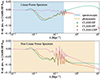 |
Fig. B.1. Ratio of the fiducial linear and nonlinear power spectrum Pmm(k, z = 0) computed using CAMB with high precision settings (CAMB :HP) to that computed using CLASS with default precision (CLASS:DP), high precision (CLASS:HP) or ultra-high precision (CLASS:UHP). In this fiducial case, the summed neutrino mass is ∑mν = 60 meV. The cyan shading denotes the range of wavenumbers probed by the spectroscopic likelihood, while the orange shading shows the range of wavenumbers for which the photometric likelihood is the most sensitive. |
Even with default precision, the difference between CAMB:HP and CLASS:DP is at most 0.1% in the linear and nonlinear spectra, that is, below the Euclid sensitivity level. Thus, it is not a surprise that MCMC forecasts performed with CLASS:DP agree with Fisher forecasts performed with CAMB:HP. However, we know that Fisher forecasts require enhanced accuracy to avoid an amplification of numerical errors when computing derivatives and inverting Fisher matrices. In the case of the photometric probes, we find that CAMB:HP and CLASS:DP settings are sufficient for computing stable derivatives and obtaining a very good match between the marginalised and unmarginalised errors derived from CF/CAMB and CF/CLASS. Switching to CLASS :HP has a marginal impact, but it tends to offer even more stability in the calculation of derivatives, with an even weaker dependence on the step sizes. To stay on the conservative side, we adopt this setting whenever using the photometric likelihood. The excellent agreement between the marginalised and unmarginalised errors obtained with CAMB :HP and CLASS :HP for this probe is illustrated by the upper panels of Figs. 6 to 8.
However, we find a slightly poorer agreement between the marginalised and unmarginalised errors obtained with CAMB:HP and CLASS:HP in the spectroscopic case (not shown here for conciseness), with differences marginally exceeding our validation threshold of 10% in some cases. Looking at various elements in the Fisher matrix, we find that this is caused by small differences in the derivatives with respect to ∑mν. After some investigation, we conclude that the below 10−3 error introduced by the CLASS neutrino fluid approximation is responsible for such small differences. Even with the enhanced setting in the last line of CLASS:HP, this approximation leads to a suppression of the matter power spectrum by 0.07% on scales between k = 10−2 h Mpc−1 and k = 2 × 10⁻¹ h Mpc−1, which is clearly visible in the upper plot of Fig. B.1. This suppression propagates to the derivative of the linear power spectrum ∂P(k, z)/∂∑mν and finally to the Fisher matrix.
We fix this issue by defining some ultra-high precision settings, CLASS:UHP, in which the neutrino fluid approximation is never used. Switching off the fluid approximation has a potential drawback. In this case, the Bolztmann hierarchy is integrated even deep inside the Hubble scale regime. As a consequence, the evolution of perturbations can be more affected by artefacts coming from the truncation of the hierarchy at ℓmax. These artefacts can be seen as an artificial reflection of power on the boundary (see for instance Hu et al. 1995; Lesgourgues & Tram 2011). Thus, the cut-off multipole must be increased accordingly. In CLASS:UHP, we set it to ℓmax = 40. Finally, in the absence of a neutrino fluid approximation, CLASS becomes much slower. We speed it up by 20% by integrating the differential equations with the evolver rkck (a Runge-Kutta evolver more optimised for highly oscillatory massive neutrino equations) instead of the default ndf15 (an implicit evolver more optimised for stiff systems, see Blas et al. 2011). All in all, this amounts to replacing the last two lines of CLASS:HP by three new lines:
With such CLASS:UHP settings, we are able to validate the Fisher matrix pipelines for the spectroscopic probe with either pessimistic or optimistic settings (see the lower panels in Figs. 6 to 8).
In summary, when using the CF/CAMB pipeline, we always use CAMB:HP settings. For the CF/CLASS and MP/Fisher pipelines, we use CLASS:HP for the photometric probe and CLASS:UHP for the spectroscopic probe. Finally, for the MP/MCMC pipeline, we always use CLASS:DP.
Appendix C: Effect of the step size for ∑mν
Due to the smallness of the effect of the summed neutrino mass on the power spectrum, we have to use larger step sizes for ∑mν than for the other parameters, to ensure that the numerical derivatives are dominated by physical effects rather than numerical noise from the EBS. For other parameters our step size is set to 1% of the fiducial value. Instead, for ∑mν, our default relative stepsize is of 10%. To check whether this choice is numerically stable, we test here the effect of using larger step sizes in the CF/CAMB pipeline, for the spectroscopic probe and with optimistic settings. The results can be seen in Fig. C.1. We find that the errors do not change by more than 3% when going from a 10% step size to a 50% step size (corresponding to step sizes of 6 meV to 30 meV). Additionally, in the 2D contour plots we checked that the directions of correlation with other cosmological parameters are preserved. This speaks again to the robustness of the derivatives. Using the CF/CLASS pipeline we find similar results, but in that case the errors remain stable even when the relative step size is lowered to a few percent only.
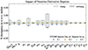 |
Fig. C.1. Effect on the marginalised and unmarginalised errors of changing the step size in the calculation of numerical derivatives with respect to the summed neutrino mass ∑mν in the CF/CAMB pipeline. We choose here the case of the spectroscopic probe with optimistic settings, and we stick to the same assumptions and precision parameters as in the rest of the validation Sect. 6. The step sizes (0.1, 0.3, 0.5) are expressed relative to the fiducial value ∑mν = 60 meV, and thus correspond to (6 meV, 18 meV, 30 meV). |
Appendix D: Effect of the nonlinear prescription
A difference between Euclid Collaboration (2024a) and this work resides in the choice of algorithm for the computation of nonlinear corrections to the power spectrum. As explained in Sect. 3.3, in the current analysis, we switched from HALOFIT to HMcode (Mead et al. 2021). As a matter of fact, the latter is closer to the results of N-body simulations, especially in the presence of massive neutrinos. In Fig. D.1 we can see the effect induced by this change on the predicted marginalised and unmarginalised errors of the ΛCDM+∑mν+Neff model. While the unmarginalised errors remain stable up to 10% variations, we see a strong difference – of as much as 70% – in the marginalised errors on Ωm, 0, σ8, ns, h, and ∑mν. The error on cosmological parameters predicted with HALOFIT are systematically lower than those obtained with HMcode. In the 2D contours of Fig. D.2 we also see that the directions of correlation between pairs of parameters are different with HALOFIT. Finally, Fig. D.3 shows that in the case of optimistic specifications if HMcode is used to generate the fiducial model – or, in other words, is assumed to account for the truth – but the fit is performed using HALOFIT, the cosmological parameters are recovered incorrectly, with up to 3 σ bias in the cosmological parameters and even more in the nuisance parameters, in agreement with Euclid Collaboration (2021b). These tests stress the high sensitivity of the Euclid pipeline to the method used to predict nonlinear corrections. In order to measure cosmological parameters, it is essential to fit the data with an extremely accurate model of nonlinear corrections.
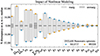 |
Fig. D.1. Difference between the marginalised and unmarginalised errors inferred from the CF/CAMB pipeline using either HALOFIT or HMcode. |
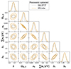 |
Fig. D.2. Marginalised posteriors and confidence contours for the same Fisher forecasts as in Fig. D.1, that is, when switching from HMcode to HALOFIT. |
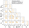 |
Fig. D.3. Biasing test, where the fiducial model is generated using HMcode and fitted using HALOFIT. |
Appendix E: Importance of using the CDM+baryons power spectrum
In Sect. 3, we stressed the importance of modelling the galaxy power spectrum as a biased tracer of the cold dark matter plus baryonic power spectrum (Castorina et al. 2014, 2015), such that on linear scales  . Here we illustrate the importance of this assumption by deliberately adopting instead the inaccurate prescription
  , where the total matter power spectrum Pmm(k; z) includes neutrino density fluctuations. At the level of a forecast, the difference between the two treatments arises not from different assumptions concerning the fiducial model, but from the different dependence of the spectrum on cosmological parameters, and particularly on the neutrino mass. Indeed, we expect that Pcc is less suppressed by neutrino free-streaming effects, such that
Thus, adopting the wrong prescription should artificially increase the sensitivity to ∑mν (and to all correlated parameters), as argued in more details in Vagnozzi et al. (2018).
This issue is relevant both for the galaxy clustering component of the photometric probe and for the spectroscopic probe. Here we choose to illustrate its importance in the case of the photometric probe with optimistic settings. In Figs. E.1 and E.2, we present a comparison between two Fisher forecasts for this probe, the first one adopting the correct approach, and the second one switching to the wrong prescription both for the fiducial and fitted models. In Fig. E.3 we present a second test based on MCMC forecasts in which we stick to the correct approach for the fiducial model, but we fit it using either the correct or the incorrect prescription.
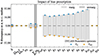 |
Fig. E.1. For the photometric probe with optimistic settings, comparison of the 1D marginalised and unmarginalised errors obtained under the assumption that the galaxy power spectrum is a biased tracer of either Pmm (incorrect modelling) or Pcc (correct modelling). For the parameter ∑mν the relative difference in the unmarginalised error goes outside the frame and is of the order of 43%. |
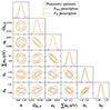 |
Fig. E.2. Marginalised posteriors and confidence contours for the same Fisher forecasts as in Fig. E.1. |
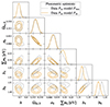 |
Fig. E.3. For the photometric probe with optimistic settings, marginalised posteriors and confidence contours from two MCMC forecasts based on the same fiducial model generated with the Pcc prescription. The mock data are then fitted either with the Pmm (incorrect modelling) or Pcc (correct modelling) prescription. |
In the first test, the unmarginalised error on ∑mν differs by 43% between the two cases (see Fig. E.1). This is a direct consequence of the different derivatives of Pcc and Pmm with respect to ∑mν. This discrepancy gets mitigated by the marginalisation over all other parameters, which reduces the difference on σ(∑mν) to about 3%. However, in the marginalised case, the error bars on the parameters that are correlated with ∑mν also increase – most noticeably for the bias parameters. As a matter of fact, the response of Pcc(k; z) to a variation in the neutrino mass is more degenerate with a change of amplitude (and thus of linear bias) than the response of Pmm(k; z). Thus, when using the wrong prescription, one underestimates the correlation between ∑mν and the bias parameters (see Fig. E.2), and artificially reduces the error not only on ∑mν but also on each bi.
In the second test, we can check that fitting the correct fiducial model with the wrong prescription leads to artificially strong constrains on ∑mν (see Fig. E.3). In this case, the theoretical model based on Pmm cannot fit perfectly the fiducial model based on Pcc: there is always a residual difference. This test is particularly interesting because it shows that the incorrect model fits this residual by a combination of a wrong ∑mν and wrong biases. This could be expected, since the difference between Pcc and Pmm is close to a constant factor over a wide range of scales, as can be checked in Fig. 1. This explains the shifted means in the ∑mν and bi posteriors visible in Fig. E.3. Looking at the ∑mν posteriors, we see that if such a mistake occurred in the analysis of real data, one would incorrectly conclude that the data prefer a vanishing neutrino mass, while in reality ∑mν = 60 meV is preferred.
Appendix F: Parameter correlations in different cosmologies
In this appendix we show additional triangle plots with the 1D marginalised posteriors and 2D confidence contours that are not shown in Sect. 7. Figure F.1 shows the results obtained in the baseline ΛCDM+∑mν model from each of the Euclid primary probes and from their combination. Figures F.2 and F.3 show the results obtained in the intermediate models (ΛCDM+∑mν+ΔNeff, and w0waCDM+∑mν, respectively) with the data combinations Euclid +Planck (orange), and Euclid +CMB-S4+LiteBIRD (green). Note that, when comparing Fig. F.1 with Fig. 13, the photometric probes (red contours) show a different direction of degeneracy between ∑mν and h, which are positively correlated in the baseline ΛCDM+∑mν model. On the other hand, when combining Euclid with CMB (Figs. F.2 and F.3), it is difficult to identify any significant change in the direction of the degeneracies in parameter space between one model and the other.
Appendix G: Correlation with bias parameters
Figures G.1 and G.2 show the correlation between the bias parameters of photometric and spectroscopic observables, respectively, and the cosmological parameters in the extended w0waCDM+∑mν+ΔNeff model. We show only two redshift bins for each observable noticing that the correlation is the same in all the redshift bins. It appears that there is no correlation between the neutrino mass and the bias parameters, either in WL+GCph + XCph or in GCsp. On the other hand, a mild anti-correlation is found between the bias parameters and ΔNeff in WL+GCph + XCph, thus arising from GCph. The reason why this correlation appears in GCph while it is not present in GCsp is that the projection of the matter power spectrum in angular harmonics and the convolution with the window function redistribute the power over a wider range of scales; the feature induced by a variation in ΔNeff on the matter power spectrum (see Fig. 2) is smoothed out and thus can be mimicked by a variation in the bias.
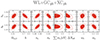 |
Fig. G.1. 2D confidence contours showing the correlation between the bias parameters of the fifth, and of the ninth redshift bins (b4 and b8) and the cosmological parameters, obtained by fitting photometric observables (WL+GCph + XCph) to the w0waCDM+∑mν+ΔNeff model. |
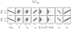 |
Fig. G.2. 2D confidence contours showing the correlation between the bias parameters of the first and of the fourth redshift bin [lnb0σ8(z0), and lnb3σ8(z3)] and the cosmological parameters, obtained by fitting spectroscopic observables (GCsp) to the w0waCDM+∑mν+ΔNeff model. |
Besides ΔNeff, the bias parameters show correlations with most cosmological parameters, highlighting the importance of a careful study of bias from simulations.
Appendix H: Impact of baryonic feedback
An accurate modelling of large scale structure observables in the nonlinear regime requires accounting for baryonic feedback effects (Semboloni et al. 2011; Parimbelli et al. 2019; Schneider et al. 2020a,b; Euclid Collaboration 2021b; Spurio Mancini & Bose 2023). Here, we test the robustness of our results on the neutrino mass sensitivity against such effects. To this end, we multiply the matter power spectrum Pmm(kℓ, z) of Eq. (4) in Sect. 3.1 by the boost factor obtained with the emulator BCemu (Giri & Schneider 2021). Note that we apply the boost factor only to Pmm(kℓ, z), thus, accounting for baryonic feedback effects only in weak lensing. We vary two BCemu parameters. The first one, log10Mc, is related to the critical mass Mc′ such that halos with a virial mass that is lower than Mc′ have a gas profile shallower than the Navarro-Frenk-White profile. Then, Mc is the dimensionless parameter such that Mc = Mc′/(1 h−1 M⊙). The second parameter is the index νontMc describing the power-law redshift dependence of Mc. This choice is motivated by the fact that log10Mc is the parameter governing the suppression of Pmm(kℓ, z), thus, it is expected to be the most correlated with the neutrino mass. Moreover, given the cut-off at ℓ = 1500 in our pessimistic specifications, including more than one free parameter for baryonic feedback might lead to an overfitting, leaving the additional parameters unconstrained. In Fig. H.1, we compare the constraints from the Euclid photometric probe on cosmological parameters obtained with and without baryonic feedback (red-filled and green-empty contours, respectively) in the w0waCDM+∑mν+ΔNeff model. We assume pessimistic specifications as in our final results of Sect. 7. We see that baryonic feedback does not have a dramatic impact on the constraints, and the critical mass parameter does not show a well defined correlation with either of the neutrino parameters. This outcome was expected since baryonic feedback effects are mostly relevant at ℓ > 1500, thus, beyond the range fitted in the pessimistic scenario. Nevertheless, the variation in the log10Mc parameter slightly degrades the sensitivity to the neutrino mass: more specifically, the 95% upper bound on ∑mν increases by about 10%. As already pointed out in Spurio Mancini & Bose (2023), if the analysis was extended to ℓ = 3000, 5000, the degradation in sensitivity to the neutrino mass due to the inclusion of baryonic feedback effects would be more dramatic.
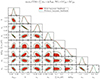 |
Fig. H.1. 1D marginalised posteriors and 2D confidence contours for cosmological parameters and for baryonic feedback parameters, obtained by fitting photometric observables (WL+GCph+XCph) to the w0waCDM+∑mν model, with and without varying baryonic feedback parameters (red-filled and green-empty contours, respectively). The contours for baryonic feedback parameters are also shown when they are varied. |
All Tables
Fiducial values of the cosmological parameters used in the validation and result sections.
Marginalised 1 σ uncertainties on cosmological parameters in ΛCDM + ∑mν, in ΛCDM + ∑mν + Neff, in w0waCDM + ∑mν, and in w0waCDM + ∑mν + ΔNeff.
All Figures
|
Fig. 1. Effects of the neutrino mass on the linear total matter (solid) or cold-plus-baryonic matter (dashed) power spectrum, presented as ratios with respect to the ΛCDM spectrum with massless neutrinos for four different values of the summed neutrino mass. Top: Singling out the effect of neutrino free-streaming, we keep the parameters {Ωm, 0h2, Ωb, 0h2, ΩΛ} fixed. Bottom: Quantities best constrained by CMB data, that is, {zeq, Ωb, 0h2, θs}, are fixed to show what is left for Euclid to measure. The mass is always equally split between the three neutrino species. |
| In the text | |
|
Fig. 2. Effect of the effective number of relativistic degrees of freedom Neff = 3.044 + ΔNeff on the linear total matter power spectrum, presented as ratios with respect to the ΛCDM spectrum with Neff = 3.044. Top: Density and Hubble parameters {Ωm, 0, Ωb, 0, h} fixed only. Bottom: Quantities best constrained by CMB data, that is, {zeq, Ωb, 0h2, θs}, are fixed to show what is left for Euclid to measure. Here, we assume only massless neutrinos. |
| In the text | |
|
Fig. 3. Relative percentage difference of the nonlinear power spectrum computed with various recipes with respect to the DEMNUni simulations for the case ∑mν = 0.16 eV. We note that here, contrary to the forecast analysis, and to be consistent with the DEMNUni simulations, we assume the total neutrino mass to be equally shared among the three neutrino species m1 = m2 = m3 = ∑mν/3. The left column shows the total matter power spectrum, while the right column shows the cold dark matter power spectrum. The spectra are evaluated at z = 0, 1, 2 (first, second and third rows, respectively). The theoretical predictions are provided by HALOFIT (dashed orange line), HMcode (solid blue line), EuclidEmulator2 (dashed red line), and BACCOemulator (dot-dashed green line). The purple shaded area represents the shot noise of the simulations, and the vertical dotted line the maximum wavenumber. In the third row the predictions of BACCOemulator are missing because the emulator is trained only up to z = 1.5. The predictions for the cold dark matter power spectrum (neglecting the contribution of neutrino perturbations) is computed according to the approximate formula Eq. (16) (see text for details). |
| In the text | |
|
Fig. 4. Theoretical predictions of the suppression of the total matter power spectrum (left) and of the cold dark matter power spectrum (right) in massive neutrino cosmologies (∑mν = 0.16 eV and ∑mν = 0.32 eV) with respect to the pure ΛCDM case with massless neutrinos at z = 0. The colour coding of the theoretical predictions is the same as in Fig. 3. In the case ∑mν = 0.32 eV, EuclidEmulator2 is not shown because the value of the neutrino mass is too far away from the range of validity of the emulator. The DEMNUni simulations are depicted as black pluses. |
| In the text | |
|
Fig. 5. Theoretical predictions of the suppression of the total matter power spectrum in non-standard Neff cosmologies with respect to the standard one, at z = 0, and assuming fixed values of {Ωm, 0, Ωb, 0, h}, like in the top panel of Fig. 2. The colour coding of the theoretical predictions is the same as in Fig. 3. We add here two more prescriptions, obtained by rescaling Ωc, 0, Ωb, 0 and h to mimic changes in Neff. We refer to it as “ΛCDM equivalent”: the dot-dashed pink line represents results for EuclidEmulator2; and the dotted cyan line represents the BACCOemulator prediction. Black crosses represent results from N-body simulations. |
| In the text | |
|
Fig. 6. For the w0waCDM model, comparison of each of the Fisher marginalised (light grey) and unmarginalised (dark grey) errors on each cosmological and nuisance parameter for: photometric optimistic probe (top left); photometric pessimistic probe (top right); spectroscopic optimistic probe (bottom left); and spectroscopic pessimistic probe (bottom right). For the spectroscopic probe the labels lbsi are short for the parameters ln(b σ8)i. |
| In the text | |
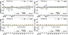 |
Fig. 7. Same as Fig. 6, but for the ΛCDM+∑mν+Neff model. |
| In the text | |
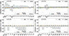 |
Fig. 8. Same as Fig. 6, but for the w0CDM+∑mν model. |
| In the text | |
|
Fig. 9. Comparison of the 1D marginalised posteriors and 2D (95% C.L. and 68% C.L.) marginalised contours obtained with the MP/MCMC pipeline to the Gaussian posteriors and elliptical contours from the FI pipelines CF/CAMB and MP/Fisher for the w0waCDM model. Left: Spectroscopic optimistic probe. Right: Photometric optimistic probe. |
| In the text | |
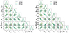 |
Fig. 10. Same as Fig. 9, but for the ΛCDM+∑mν+Neff model. |
| In the text | |
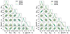 |
Fig. 11. Same as Fig. 9, but for the w0CDM model+∑mν model. |
| In the text | |
|
Fig. 12. Sensitivity (relative errors with respect to the fiducial values) to the cosmological parameters, comparing ΛCDM cosmologies (solid colour bars) and w0waCDM cosmologies (hatched colour bars), for models with (bottom panel) and without (top panel) varying Neff. The different colours correspond to the sensitivity of different data combinations: WL+GCph+XCph+GCsp (blue); Euclid +Planck (orange); and Euclid +CMB-S4+LiteBIRD (green). We note that for wa we show the absolute errors, while for ΔNeff we show the 95% upper limits. For the neutrino mass we always show the relative 1 σ uncertainty as computed from the posterior variance in order to facilitate the comparison between different data sets. |
| In the text | |
|
Fig. 13. Marginalised 1D distribution (diagonal) and 2D (off-diagonal) 68% and 95% contours for a selection of parameters of the w0waCDM+∑mν+Neff model obtained by fitting GCsp (grey), WL+GCph+XCph (red), and their combination (blue). The horizontal and vertical dashed lines mark the fiducial values. |
| In the text | |
|
Fig. 14. Marginalised 1D distributions (diagonal) and 2D (off-diagonal) 68% and 95% contours for a selection of parameters of the w0waCDM+∑mν+Neff model obtained by fitting Euclid +Planck (orange), and Euclid +CMB-S4+LiteBIRD (green). The horizontal and vertical dashed lines mark the fiducial values. |
| In the text | |
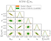 |
Fig. 15. Same as Fig. 14, but for the ΛCDM+∑mν model. |
| In the text | |
|
Fig. 16. Marginalised 2D contours of ∑mν and τreio for the ΛCDM+∑mν model. |
| In the text | |
|
Fig. 17. Sum of neutrino masses ∑mν in the inverted ordering (red solid line) scenarios and in the normal ordering (blue solid line), including the uncertainties on the mass squared differences from oscillation experiments, as a function of the lightest neutrino mass. The grey dot-dashed lines show the 95% CL upper bounds from Planck only (dark grey), and in combination with external data (Planck +ext., light grey). For the latter we use the value quoted in Alam et al. (2021) for Planck +Pantheon-SNe+SDSS(BAO+RSD)+DES 3 × 2pt, which includes Planck, Pantheon type Ia supernovae, baryon acoustic oscillations and redshift-space distortions from the Sloan Digital Sky Survey, and weak lensing measurements from the Dark Energy Survey. The region above the blue dashed line is excluded at 95% CL by Euclid only primary probes. The orange shading shows the 68% and 95% CL limits on ∑mν from Euclid +Planck in the baseline ΛCDM+∑mν model, assuming a fiducial value ∑mν = 60 meV. The 68% and 95% CL constraints from Euclid +CMB-S4+LiteBIRD are shown in green. We note that we split the two constraints into two different ranges of the lightest neutrino mass only to avoid an overlap of the two shadings. Assuming that the true value of the neutrino mass sum is indeed the minimum allowed by neutrino oscillation experiments in normal ordering, the combination Euclid +CMB-S4+LiteBIRD will rule out the inverted ordering at 2.5 σ. |
| In the text | |
|
Fig. 18. Contribution of new light particles beyond the Standard Model to ΔNeff as a function of their decoupling temperature. Assuming natural units, we report the temperatures in GeV. As a reference we show the contribution of a Goldstone boson (solid brown line), a Weyl fermion (solid red line), and a massless Gauge boson (solid purple line). The grey vertical bands denote the range of temperatures of the QCD phase transition (around 200 MeV) and neutrino decoupling (around 1 MeV), while the thin grey vertical lines mark the annihilation temperature of Standard Model particles. The grey horizontal dot-dashed line represents the current 95% CL limit from Planck TT,TE,EE+lensing+BAO (Planck Collaboration VI 2020). The horizontal dashed lines mark the 95% upper bounds on ΔNeff from Euclid only (in blue) and in combination with current (Planck) and future (CMB-S4+LiteBIRD) CMB surveys (in orange and green, respectively). As explained in Sect. 4.2, we choose to adopt more conservative assumptions regarding the CMB-S4 sensitivity and foreground removal than in a similar figure in the CMB-S4 white paper, Fig. 23 of Abazajian et al. (2016). |
| In the text | |
|
Fig. A.1. Effect on the marginalised and unmarginalised errors of changing the numerical derivative method from 3PT to 4PT_FWD in the CF/CAMB pipeline. Here we choose the case of the spectroscopic probe with optimistic settings, and we stick to the same assumptions and precision parameters as in the rest of the validation (Sect. 6). In this test, the nuisance parameters are kept fixed for simplicity. The marginalisation takes place over other cosmological parameters. |
| In the text | |
|
Fig. B.1. Ratio of the fiducial linear and nonlinear power spectrum Pmm(k, z = 0) computed using CAMB with high precision settings (CAMB :HP) to that computed using CLASS with default precision (CLASS:DP), high precision (CLASS:HP) or ultra-high precision (CLASS:UHP). In this fiducial case, the summed neutrino mass is ∑mν = 60 meV. The cyan shading denotes the range of wavenumbers probed by the spectroscopic likelihood, while the orange shading shows the range of wavenumbers for which the photometric likelihood is the most sensitive. |
| In the text | |
|
Fig. C.1. Effect on the marginalised and unmarginalised errors of changing the step size in the calculation of numerical derivatives with respect to the summed neutrino mass ∑mν in the CF/CAMB pipeline. We choose here the case of the spectroscopic probe with optimistic settings, and we stick to the same assumptions and precision parameters as in the rest of the validation Sect. 6. The step sizes (0.1, 0.3, 0.5) are expressed relative to the fiducial value ∑mν = 60 meV, and thus correspond to (6 meV, 18 meV, 30 meV). |
| In the text | |
|
Fig. D.1. Difference between the marginalised and unmarginalised errors inferred from the CF/CAMB pipeline using either HALOFIT or HMcode. |
| In the text | |
|
Fig. D.2. Marginalised posteriors and confidence contours for the same Fisher forecasts as in Fig. D.1, that is, when switching from HMcode to HALOFIT. |
| In the text | |
|
Fig. D.3. Biasing test, where the fiducial model is generated using HMcode and fitted using HALOFIT. |
| In the text | |
|
Fig. E.1. For the photometric probe with optimistic settings, comparison of the 1D marginalised and unmarginalised errors obtained under the assumption that the galaxy power spectrum is a biased tracer of either Pmm (incorrect modelling) or Pcc (correct modelling). For the parameter ∑mν the relative difference in the unmarginalised error goes outside the frame and is of the order of 43%. |
| In the text | |
|
Fig. E.2. Marginalised posteriors and confidence contours for the same Fisher forecasts as in Fig. E.1. |
| In the text | |
|
Fig. E.3. For the photometric probe with optimistic settings, marginalised posteriors and confidence contours from two MCMC forecasts based on the same fiducial model generated with the Pcc prescription. The mock data are then fitted either with the Pmm (incorrect modelling) or Pcc (correct modelling) prescription. |
| In the text | |
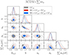 |
Fig. F.1. Same as Fig. 13, but for the baseline ΛCDM+∑mν model. |
| In the text | |
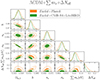 |
Fig. F.2. Same as Fig. 15, but for the ΛCDM+∑mν+ΔNeff model. |
| In the text | |
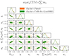 |
Fig. F.3. Same as Fig. 15, but for the w0waCDM+∑mν model. |
| In the text | |
|
Fig. G.1. 2D confidence contours showing the correlation between the bias parameters of the fifth, and of the ninth redshift bins (b4 and b8) and the cosmological parameters, obtained by fitting photometric observables (WL+GCph + XCph) to the w0waCDM+∑mν+ΔNeff model. |
| In the text | |
|
Fig. G.2. 2D confidence contours showing the correlation between the bias parameters of the first and of the fourth redshift bin [lnb0σ8(z0), and lnb3σ8(z3)] and the cosmological parameters, obtained by fitting spectroscopic observables (GCsp) to the w0waCDM+∑mν+ΔNeff model. |
| In the text | |
|
Fig. H.1. 1D marginalised posteriors and 2D confidence contours for cosmological parameters and for baryonic feedback parameters, obtained by fitting photometric observables (WL+GCph+XCph) to the w0waCDM+∑mν model, with and without varying baryonic feedback parameters (red-filled and green-empty contours, respectively). The contours for baryonic feedback parameters are also shown when they are varied. |
| In the text | |
Current usage metrics show cumulative count of Article Views (full-text article views including HTML views, PDF and ePub downloads, according to the available data) and Abstracts Views on Vision4Press platform.
Data correspond to usage on the plateform after 2015. The current usage metrics is available 48-96 hours after online publication and is updated daily on week days.
Initial download of the metrics may take a while.