| Issue |
A&A
Volume 682, February 2024
|
|
|---|---|---|
| Article Number | A90 | |
| Number of page(s) | 33 | |
| Section | Numerical methods and codes | |
| DOI | https://doi.org/10.1051/0004-6361/202346772 | |
| Published online | 08 February 2024 | |
Euclid: Validation of the MontePython forecasting tools★
1
Institute for Theoretical Particle Physics and Cosmology (TTK), RWTH Aachen University,
52056
Aachen,
Germany
e-mail: This email address is being protected from spambots. You need JavaScript enabled to view it.
2
Institut de Ciències del Cosmos (ICCUB), Universitat de Barcelona (IEEC-UB),
Martí i Franqueès 1,
08028
Barcelona,
Spain
3
Hamburger Sternwarte, University of Hamburg,
Gojenbergsweg 112,
21029
Hamburg,
Germany
4
Physikalisches Institut, Ruprecht-Karls-Universität Heidelberg,
Im Neuenheimer Feld 226,
69120
Heidelberg,
Germany
5
Dipartimento di Fisica “Aldo Pontremoli”, Universitá degli Studi di Milano,
Via Celoria 16,
20133
Milano,
Italy
6
IFPU - Institute for Fundamental Physics of the Universe,
Via Beirut 2,
34151
Trieste,
Italy
7
SISSA – International School for Advanced Studies,
Via Bonomea 265,
34136
Trieste TS,
Italy
8
INAF–Osservatorio Astronomico di Trieste,
Via G. B. Tiepolo 11,
34143
Trieste,
Italy
9
INFN - Sezione di Trieste,
Via Valerio 2,
34127
Trieste TS,
Italy
10
Université Libre de Bruxelles (ULB), Service de Physique Théorique CP225,
Boulevard du Triomphe,
1050
Bruxelles,
Belgium
11
Department of Physics “E. Pancini”, University Federico II,
Via Cinthia 6,
80126
Napoli,
Italy
12
INAF-Osservatorio Astronomico di Roma,
Via Frascati 33,
00078
Monteporzio Catone,
Italy
13
INFN-Sezione di Roma, Piazzale Aldo Moro,
2 – c/o Dipartimento di Fisica, Edificio G. Marconi,
00185
Roma,
Italy
14
Dipartimento di Fisica, Universitá degli Studi di Torino,
Via P. Giuria 1,
10125
Torino,
Italy
15
INFN-Sezione di Torino,
Via P. Giuria 1,
10125
Torino,
Italy
16
INAF-Osservatorio Astrofisico di Torino,
Via Osservatorio 20,
10025
Pino Torinese (TO),
Italy
17
Departamento de Física, FCFM, Universidad de Chile,
Blanco Encalada
2008,
Santiago,
Chile
18
Université Saint-Joseph; Faculty of Sciences,
Beirut,
Lebanon
19
Institut für Theoretische Physik, University of Heidelberg,
Philosophenweg 16,
69120
Heidelberg,
Germany
20
Institut de Recherche en Astrophysique et Planétologie (IRAP), Université de Toulouse, CNRS, UPS, CNES,
14 Av. Édouard Belin,
31400
Toulouse,
France
21
Dipartimento di Fisica e Scienze della Terra, Universitá degli Studi di Ferrara,
Via Giuseppe Saragat 1,
44122
Ferrara,
Italy
22
Istituto Nazionale di Fisica Nucleare, Sezione di Ferrara,
Via Giuseppe Saragat 1,
44122
Ferrara,
Italy
23
INAF – IASF Milano,
Via Alfonso Corti 12,
20133
Milano,
Italy
24
Université Paris-Saclay, CNRS/IN2P3, IJCLab,
91405
Orsay,
France
25
Centre National d’Études Spatiales – Centre spatial de Toulouse,
18 avenue Édouard Belin,
31401
Toulouse Cedex 9,
France
26
Jet Propulsion Laboratory, California Institute of Technology,
4800 Oak Grove Drive,
Pasadena,
CA,
91109,
USA
27
Université Paris-Saclay, Université Paris Cité, CEA, CNRS, Astrophysique, Instrumentation et Modélisation Paris-Saclay,
91191
Gif-sur-Yvette,
France
28
Université Paris-Saclay, CNRS, Institut d’Astrophysique spatiale,
91405
Orsay,
France
29
Institute of Cosmology and Gravitation, University of Portsmouth,
Portsmouth
PO1 3FX,
UK
30
INAF-Osservatorio di Astrofisica e Scienza dello Spazio di Bologna,
Via Piero Gobetti 93/3,
40129
Bologna,
Italy
31
Dipartimento di Fisica e Astronomia “Augusto Righi” - Alma Mater Studiorum Università di Bologna,
Via Piero Gobetti 93/2,
40129
Bologna,
Italy
32
INFN-Sezione di Bologna,
Viale Berti Pichat 6/2,
40127
Bologna,
Italy
33
Dipartimento di Fisica, Università di Genova,
Via Dodecaneso 33,
16146
Genova,
Italy
34
INFN-Sezione di Genova,
Via Dodecaneso 33,
16146
Genova,
Italy
35
INAF-Osservatorio Astronomico di Capodimonte,
Via Moiariello 16,
80131
Napoli,
Italy
36
Instituto de Astrofísica e Ciências do Espaço, Universidade do Porto, CAUP, Rua das Estrelas,
4150-762
Porto,
Portugal
37
Institut de Física d’Altes Energies (IFAE), The Barcelona Institute of Science and Technology,
Campus UAB,
08193
Bellaterra (Barcelona),
Spain
38
Port d’Informació Científica,
Campus UAB, C. Albareda s/n,
08193
Bellaterra (Barcelona),
Spain
39
INFN section of Naples,
Via Cinthia 6,
80126
Napoli,
Italy
40
Dipartimento di Fisica e Astronomia “Augusto Righi” – Alma Mater Studiorum Universitá di Bologna,
Viale Berti Pichat 6/2,
40127
Bologna,
Italy
41
Institut national de physique nucléaire et de physique des particules,
3 rue Michel-Ange,
75794
Paris Cedex 16,
France
42
Institute for Astronomy, University of Edinburgh,
Royal Observatory, Blackford Hill,
Edinburgh
EH9 3HJ,
UK
43
European Space Agency/ESRIN,
Largo Galileo Galilei 1,
00044
Frascati,
Roma,
Italy
44
ESAC/ESA,
Camino Bajo del Castillo, s/n., Urb. Villafranca del Castillo,
28692
Villanueva de la Cañada,
Madrid,
Spain
45
University of Lyon, Univ. Claude-Bernard Lyon-1 CNRS/IN2P3, IP2I Lyon, UMR 5822,
69622
Villeurbanne,
France
46
Institute of Physics, Laboratory of Astrophysics, École Polytechnique Fédérale de Lausanne (EPFL),
Observatoire de Sauverny,
1290
Versoix,
Switzerland
47
Mullard Space Science Laboratory, University College London,
Holmbury St Mary, Dorking,
Surrey
RH5 6NT,
UK
48
Department of Astronomy, University of Geneva,
Ch. d’Ecogia 16,
1290
Versoix,
Switzerland
49
Instituto de Astrofísica e Ciências do Espaço, Faculdade de Ciências, Universidade de Lisboa,
Campo Grande,
1749-016
Lisboa,
Portugal
50
Departamento de Física, Faculdade de Ciências, Universidade de Lisboa,
Edifício C8, Campo Grande,
1749-016
Lisboa,
Portugal
51
INFN-Padova,
Via Marzolo 8,
35131
Padova,
Italy
52
INAF-Osservatorio Astronomico di Padova,
Via dell’Osservatorio 5,
35122
Padova,
Italy
53
Max Planck Institute for Extraterrestrial Physics,
Giessenbachstr. 1,
85748
Garching,
Germany
54
University Observatory, Faculty of Physics, Ludwig-Maximilians-Universität,
Scheinerstr. 1,
81679
Munich,
Germany
55
Institute of Theoretical Astrophysics, University of Oslo,
PO Box 1029
Blindern,
0315
Oslo,
Norway
56
von Hoerner & Sulger GmbH,
SchloßPlatz 8,
68723
Schwetzingen,
Germany
57
Technical University of Denmark,
Elektrovej 327,
2800
Kgs. Lyngby,
Denmark
58
Cosmic Dawn Center (DAWN),
Elektrovej
327,
Denmark
59
Max-Planck-Institut für Astronomie,
Königstuhl 17,
69117
Heidelberg,
Germany
60
Universitäts-Sternwarte München, Fakultät für Physik, Ludwig-Maximilians-Universität München,
Scheinerstrasse 1,
81679
München,
Germany
61
Université de Genève, Département de Physique Théorique and Centre for Astroparticle Physics,
24 quai Ernest-Ansermet,
1211
Geneva 4,
Switzerland
62
Department of Physics,
PO Box 64,
00014
University of Helsinki,
Finland
63
Helsinki Institute of Physics, Gustaf Hällströmin katu 2, University of Helsinki,
Helsinki,
Finland
64
NOVA optical infrared instrumentation group at ASTRON,
Oude Hoogeveensedijk 4,
7991 PD
Dwingeloo,
The Netherlands
65
Argelander-Institut für Astronomie, Universität Bonn,
Auf dem Hügel 71,
53121
Bonn,
Germany
66
Department of Physics, Institute for Computational Cosmology, Durham University,
South Road,
DH1 3LE,
UK
67
Université Paris Cité, CNRS,
Astroparticule et Cosmologie,
75013
Paris,
France
68
European Space Agency/ESTEC,
Keplerlaan 1,
2201 AZ
Noordwijk,
The Netherlands
69
Department of Physics and Astronomy, University of Aarhus,
Ny Munkegade 120,
8000
Aarhus C,
Denmark
70
Centre for Astrophysics, University of Waterloo,
Waterloo,
Ontario
N2L 3G1,
Canada
71
Department of Physics and Astronomy, University of Waterloo,
Waterloo,
Ontario
N2L 3G1,
Canada
72
Perimeter Institute for Theoretical Physics,
Waterloo,
Ontario
N2L 2Y5,
Canada
73
AIM, CEA, CNRS, Université Paris-Saclay, Université de Paris,
91191
Gif-sur-Yvette,
France
74
Université Paris-Saclay, Université Paris Cité, CEA, CNRS, AIM,
91191
Gif-sur-Yvette,
France
75
Space Science Data Center, Italian Space Agency,
Via del Politecnico snc,
00133
Roma,
Italy
76
Institute of Space Science,
Str. Atomistilor, nr. 409 Măgurele,
Ilfov,
077125,
Romania
77
Dipartimento di Fisica e Astronomia “G. Galilei”, Universitá di Padova,
Via Marzolo 8,
35131
Padova,
Italy
78
Dipartimento di Fisica e Astronomia, Universitá di Bologna,
Via Gobetti 93/2,
40129
Bologna,
Italy
79
Aix-Marseille Université, CNRS/IN2P3, CPPM,
13388
Marseille,
France
80
Institut d’Estudis Espacials de Catalunya (IEEC),
Carrer Gran Capitá 2-4,
08034
Barcelona,
Spain
81
Institut de Ciencies de l’Espai (IEEC-CSIC), Campus UAB,
Carrer de Can Magrans, s/n Cerdanyola del Vallés,
08193
Barcelona,
Spain
82
Aix-Marseille Université, CNRS, CNES, LAM,
13388
Marseille,
France
83
Centro de Investigaciones Energéticas, Medioambientales y Tecnológicas (CIEMAT),
Avenida Complutense 40,
28040
Madrid,
Spain
84
Instituto de Astrofísica e Ciências do Espaço, Faculdade de Ciên-cias, Universidade de Lisboa,
Tapada da Ajuda,
1349-018
Lisboa,
Portugal
85
Universidad Politécnica de Cartagena, Departamento de Electrónica y Tecnología de Computadoras,
Plaza del Hospital 1,
30202
Cartagena,
Spain
86
Kapteyn Astronomical Institute, University of Groningen,
PO Box 800,
9700 AV
Groningen,
The Netherlands
87
INFN-Bologna,
Via Irnerio 46,
40126
Bologna,
Italy
88
Infrared Processing and Analysis Center, California Institute of Technology,
Pasadena,
CA
91125,
USA
89
Institut d’Astrophysique de Paris,
98bis Boulevard Arago,
75014
Paris,
France
90
Junia, EPA department,
41 Bd Vauban,
59800
Lille,
France
91
INAF-Osservatorio Astronomico di Brera,
Via Brera 28,
20122
Milano,
Italy
92
INFN-Sezione di Milano,
Via Celoria 16,
20133
Milano,
Italy
Received:
28
April
2023
Accepted:
6
August
2023
Abstract
Context. The Euclid mission of the European Space Agency will perform a survey of weak lensing cosmic shear and galaxy clustering in order to constrain cosmological models and fundamental physics.
Aims. We expand and adjust the mock Euclid likelihoods of the MontePython software in order to match the exact recipes used in previous Euclid Fisher matrix forecasts for several probes: weak lensing cosmic shear, photometric galaxy clustering, the cross-correlation between the latter observables, and spectroscopic galaxy clustering. We also establish which precision settings are required when running the Einstein–Boltzmann solvers CLASS and CAMB in the context of Euclid.
Methods. For the minimal cosmological model, extended to include dynamical dark energy, we perform Fisher matrix forecasts based directly on a numerical evaluation of second derivatives of the likelihood with respect to model parameters. We compare our results with those of previously validated Fisher codes using an independent method based on first derivatives of the Euclid observables.
Results. We show that such MontePython forecasts agree very well with previous Fisher forecasts published by the Euclid Collab oration, and also, with new forecasts produced by the CosmicFish code, now interfaced directly with the two Einstein–Boltzmann solvers CAMB and CLASS. Moreover, to establish the validity of the Gaussian approximation, we show that the Fisher matrix marginal error contours coincide with the credible regions obtained when running Monte Carlo Markov chains with MontePython while using the exact same mock likelihoods.
Conclusions. The new Euclid forecast pipelines presented here are ready for use with additional cosmological parameters, in order to explore extended cosmological models.
Key words: cosmology: theory / surveys / cosmology: observations / large-scale structure of Universe / cosmological parameters
This paper is published on behalf of the Euclid Consortium.
© The Authors 2024
 Open Access article, published by EDP Sciences, under the terms of the Creative Commons Attribution License (https://creativecommons.org/licenses/by/4.0), which permits unrestricted use, distribution, and reproduction in any medium, provided the original work is properly cited.
This article is published in open access under the Subscribe to Open model. This email address is being protected from spambots. You need JavaScript enabled to view it. to support open access publication.
1 Introduction
Forecasts for large-scale structure surveys are useful, first, for predicting the sensitivity of future experiments to cosmological models and parameters, and second, for paving the way to the analysis of real data. After the publication of many independent Euclid-like forecasts, an effort was undertaken within the Euclid Collaboration to compare several forecasting pipelines and validate them across each other. This has led to the publication of Euclid Collaboration (2020, ‘Euclid preparation: VII’, hereafter EP:VII).
EP:VII presents a comparison of Fisher forecasts, based on the calculation of the Fisher information matrix. This method provides a good approximation to the true experimental sensitivity as long as the posterior is nearly Gaussian, that is, as long as the likelihood is a nearly Gaussian function of model parameters (for fixed fiducial data and assuming flat priors on model parameters). Fisher matrices can be tricky to compute because they involve a calculation of derivatives with a finite difference method. The results may depend on the choice of algorithm and stepsizes because of two factors: (i) numerical noise in the theory codes and Fisher matrix codes lead to unstable derivatives in the small stepsize limit, and (ii) the posterior may deviate from a multivariate Gaussian. EP:VII shows how to mitigate these issues and obtains a very good level of agreement between several Fisher matrix codes. We choose one of them, CosmicFish (Raveri et al. 2016), as a representative case of EP:VII codes. In this work, we validated a handful of new pipelines by comparing them directly with CosmicFish.
In order to compare different Fisher matrix codes in nearly ideal conditions, one can make a strategical choice. First, compute theory predictions in advance at various points in parameter space using an Einstein–Boltzmann Solver (EBS) and store the results in files. Secondly, let different Fisher matrix codes read these data and compute the Fisher matrix with their own algorithm. This strategy is the one adopted in EP:VII with theory predictions usually computed by the EBS CAMB (Lewis et al. 2000)1.
This approach is very well suited for the cross-comparison of several Fisher matrix codes, but not for testing the impact of different EBSs. One of the intermediate goals of this work is to achieve such a task. We compared CosmicFish results when the code reads some files produced either by CAMB or CLASS (Lesgourgues 2011a; Blas et al. 2011 ). We found very good agreement between these two choices. We also provide a discussion of the settings that need to be imposed to each code in order to get stable, accurate, and mutually agreeing results.
The strategy described above relies on the storage of the data containing theoretical predictions in some files. This was a rational attitude for the purpose of comparing different Fisher matrix codes. However, once Fisher matrix codes have been validated, the need to run EBSs separately and to fill up a directory with a substantial amount of data appears as relatively heavy. Ideally, one would like to call the EBS on the fly from the Fisher code in order to save time and memory. Another intermediate goal of the current work is to implement this possibility in CosmicFish. We validated forecasts in which CosmicFish calls either CAMB or CLASS on the fly.
The Gaussian posterior approximation breaks in the case of parameters with asymmetric error bars, with a posterior hitting the prior edge (e.g. for parameters that are always positive and whose best-fit value is close to zero), or in presence of a strong nonlinear degeneracy between parameters. In order to go beyond the Gaussian approximation, it is necessary to explore directly the full likelihood instead of just its second derivatives computed at the best-fit point. This is often done using Bayesian inference algorithms – such as, for instance, the Metropolis-Hastings algorithm – involving Monte Carlo Markov chains (MCMCs). Such MCMCs require a direct coding of the likelihood ℒ unlike Fisher matrix codes such as CosmicFish that require the coding of its second derivatives, that is, of formulas in which the full likelihood itself does not appear explicitly.
Euclid forecasts based on an MCMC approach were performed earlier in a few papers (Audren et al. 2013b; Sprenger et al. 2019; Brinckmann et al. 2019) using the framework of the MontePython Bayesian inference package (Audren et al. 2013a; Brinckmann & Lesgourgues 2019). However, the Euclid recipes used in these works were never accurately compared to those validated in EP:VII.
An advantage of the MontePython package is that, once the mock likelihood describing an experiment has been implemented, it is possible to run MontePython either in Fisher mode or in MCMC mode. The former mode estimates the Fisher matrix directly from the likelihood evaluated at a few points in the vicinity of the best fit (for details see Brinckmann & Lesgourgues 2019). The MCMC mode allows for more reliable forecasts beyond the Gaussian approximation. It is important to stress that both methods rely on the numerical implementation of the likelihood formula in a single place in the code. Thus, once the likelihood has been validated in one mode, it can be considered as equally valid in the other mode. In our case, we can validate the MontePython Euclid likelihoods against the forecasts of EP:VII by running MontePython (MP) in Fisher mode (referred to as MP/Fisherfrom now on), and then, if needed, use the same likelihoods in the MontePython MCMC mode (which we call MP/MCMC). As such, MontePython is a valuable tool to transition from reliable Fisher forecasts to reliable MCMC forecasts.
One of the main goals of this paper is actually to validate the MP/Fisher Euclid pipeline against EP:VII pipelines, for the same cosmological model as in EP:VII, that is, the minimal ΛCDM model extended to dark energy with two equation-of-state parameters w0 and wa – usually referred as the Chevallier–Polarski–Linder (CPL) model (Chevallier & Polarski 2001; Linder 2003). This validation has established that the MontePython Euclid likelihoods contain exactly the same modelling of Euclid data as EP:VII, and can thus be used for robust forecasts in both MP/Fisher and MP/MCMC modes. Note that MontePython can be readily used with all the free parameters of all the cosmological models implemented in the CLASS code. Thus, this validation is an important step for cosmologists who want to produce robust Euclid forecasts in essentially whatever extended cosmological model with or without the Fisher approximation.
However, we should stress that the MontePython mock Euclid likelihoods used within this paper should not be confused with the official Euclid likelihood meant to be used with real data, that is currently under development within the Euclid Collaboration. At this stage, the MontePython likelihoods are only meant for forecasting purposes. They do not account for the state of the art in the modelling of theoretical and instrumental effects within the Euclid Collaboration.
In Sect. 2 we discuss the general analytic form of the likelihood and of the Fisher matrix assumed in EP:VII codes –such as CosmicFish – and in MontePython. These expressions rely on the same observable power spectra describing the data at the level of two-point statistics. In Sect. 3 we provide more details on the calculation of these observable power spectra, taking into account nonlinear corrections and instrumental errors. In Sect. 4 we compare five ways to compute the Fisher matrix with either CosmicFish or MontePython. In Sect. 5 we summarise our results for the sensitivity of Euclid to the parameters of the ΛCDM+{w0, wa} model, showing also the results of a MontePython MCMC forecast for comparison. In Sect. 6 we discuss the importance of correctly setting the input parameters of CAMB or CLASS in order to get consistent and robust results – showing in particular that precision settings need to be carefully handled in CAMB. We present our conclusions in Sect. 7.
2 Likelihood-based Fisher matrices
Forecasts for cosmological surveys are often based on the Fisher matrix formalism. In a Bayesian context the Fisher matrix describes the curvature of the logarithm of the likelihood ℒ in the vicinity of the best fit2.
 (1)
(1)
where {α, β} are the model (cosmological or nuisance) parameter indices. The Fisher matrix provides an accurate representation of the true likelihood only if the latter is close to being Gaussian, but it is fast to evaluate compared to a full MCMC forecast. In the presence of strong degeneracies among the parameters and highly non-Gaussian likelihoods, the Fisher matrix results may depend heavily on the steps used to evaluate numerical derivatives and may differ significantly from MCMC results. However, in the case of a sufficiently Gaussian posterior, the inverse of the Fisher matrix can be used to estimate confidence ellipses for pairs of parameters and confidence intervals for individual parameters. The present work confirms that for forecasts on the sensitivity of Euclid to the parameters of the ΛCDM+{w0, wa} model the Fisher formalism is applicable.
2.1 Photometric surveys
In a usual analysis of the photometric surveys of weak lens-ing (WL) and galaxy clustering (GCph), the observed3 signal is decomposed into spherical harmonic coefficients  in each redshift bin i. In many analyses, these coefficients are modelled to be Gaussian distributed with a covariance matrix
  . In a realistic universe this only captures a part of the information contained within the signal, but within this work we are not concerned with the analysis of other higher order statistics (such as for example the bi- or trispectrum, void or peak counts). Furthermore, it is often presumed that a reduced analyzed fraction of the sky fsky < 1 causes a corresponding proportional decrease in the covariance matrix. This leads to the likelihood
![Mathematical equation: ${\cal L} = \prod\limits_{\ell m} {{1 \over {\sqrt {\det \,C_\ell ^{{\rm{th}}}} }}{e^{ - {f_{{\rm{sky}}}}{1 \over 2}\sum\nolimits_{ij} {a_i^{{\rm{fid}}}} \left( {\ell ,m} \right){{\left( {C_{ij}^{{\rm{th}}}} \right)}^{ - 1}}\left( \ell \right)\left[ {a_j^{{\rm{fid}}}\left( {\ell ,m} \right)} \right]*}}} ,$](/articles/aa/full_html/2024/02/aa46772-23/aa46772-23-eq4.png) (2)
(2)
where the indices {i, j} run over each bin of each probe, while 𝒩 is the likelihood normalization factor. Using the fact that the observed covariance can be estimated via ![Mathematical equation: $C_{ij}^{{\rm{fid}}}(\ell ) = {1 \over {2\ell + 1}}\sum\limits_m {a_i^{{\rm{fid}}}} (\ell ,m){\left[ {a_j^{{\rm{fid}}}(\ell ,m)} \right]^*}$](/articles/aa/full_html/2024/02/aa46772-23/aa46772-23-eq5.png) , a few steps of algebra lead to
, a few steps of algebra lead to
![Mathematical equation: $\eqalign{ & {\chi ^2} \equiv - 2\ln {{\cal L} \over {{{\cal L}_{{\rm{max }}}}}} = {f_{{\rm{sky }}}}\sum\limits_\ell {(2\ell + 1)} \cr & \,\,\,\,\,\,\,\,\,\,\, \times \left\{ {\ln \left[ {{{\det {{\rm{C}}^{{\rm{th }}}}(\ell )} \over {\det {{\rm{C}}^{{\rm{fid }}}}(\ell )}}} \right] + {\mathop{\rm Tr}\nolimits} \left[ {{{\left( {{{\rm{C}}^{{\rm{th }}}}} \right)}^{ - 1}}(\ell ){{\rm{C}}^{{\rm{fid }}}}(\ell )} \right] - N} \right\}, \cr} $](/articles/aa/full_html/2024/02/aa46772-23/aa46772-23-eq6.png) (3)
(3)
where 𝒩 is the size of each C(ℓ) matrix. From here, two possible steps can be taken. Either one follows the definition of Eq. (1) to derive the Fisher matrix or one derives a more compact expression of the likelihood. The latter approach leads to
 (4)
(4)
with
![Mathematical equation: $d_\ell ^{{\rm{th}}} = \det \left[ {C_{ij}^{{\rm{th}}}(\ell )} \right],$](/articles/aa/full_html/2024/02/aa46772-23/aa46772-23-eq8.png) (5)
(5)
![Mathematical equation: $d_\ell ^{{\rm{fid}}} = \det \left[ {C_{ij}^{{\rm{fid}}}(\ell )} \right],$](/articles/aa/full_html/2024/02/aa46772-23/aa46772-23-eq9.png) (6)
(6)
![Mathematical equation: $d_\ell ^{{\rm{mix}}} = \sum\limits_k {\det } \left[ {\left\{ {\matrix{ {C_{ij}^{{\rm{th}}}(\ell )} \hfill & {{\rm{ if }}j \ne k} \hfill \cr {C_{ij}^{{\rm{fid}}}(\ell )} \hfill & {{\rm{ if }}j = k} \hfill \cr } } \right.} \right].$](/articles/aa/full_html/2024/02/aa46772-23/aa46772-23-eq10.png) (7)
(7)
In the last definition k is an index running over each bin of each probe and thus over each column of the theory matrix Cth. In each term of the sum the determinant is evaluated over a matrix such that the kth column of the theory matrix Cth has been substituted by one column of the fiducial matrix Cfid.
The likelihood of Eq. (3) can also be used to derive an expression for the Fisher matrix by differentiating twice with respect to an arbitrary pair of parameters of indices {α, β} and evaluating at the fiducial. Then we find a well-known compact expression for the Fisher matrix (Carron 2013; EP:VII)
![Mathematical equation: $\eqalign{ & {F_{\alpha \beta }} = {1 \over 2}{f_{{\rm{sky }}}}\sum\limits_\ell ( 2\ell + 1){\mathop{\rm Tr}\nolimits} \left\{ {{{\left[ {{{\rm{C}}^{{\rm{fid }}}}(\ell )} \right]}^{ - 1}}} \right.\left[ {{{\left. {{\partial _\alpha }{{\rm{C}}^{{\rm{th }}}}(\ell )} \right|}_{{\rm{fid }}}}} \right] \cr & & & & \,\,\,\,\,\,\,\left. {{{\left[ {{{\rm{C}}^{{\rm{fid }}}}(\ell )} \right]}^{ - 1}}\left[ {{{\left. {{\partial _\beta }{{\rm{C}}^{{\rm{th }}}}(\ell )} \right|}_{{\rm{fid }}}}} \right]} \right\}, \cr} $](/articles/aa/full_html/2024/02/aa46772-23/aa46772-23-eq11.png) (8)
(8)
where we omitted redshift bin indices for concision. All derivatives are evaluated precisely at the fiducial model4.
2.2 Spectroscopic surveys
Similarly, for galaxy clustering data in a spectroscopic survey (GCs) the likelihood is commonly assumed to be Gaussian with respect to the observed galaxy power spectrum Pobs(k,µ, z), such that χ2 = −2 ln(ℒ/ℒmax) reads
![Mathematical equation: $\eqalign{ & {\chi ^2} \equiv - 2\ln {{\cal L} \over {{{\cal L}_{\max }}}} = \sum\limits_i {\int {{k^2}} } {\rm{d}}k\int {\rm{d}} \mu {{V_i^{{\rm{fid}}}} \over {8{\pi ^2}}} \cr & \,\,\,\,\,\,\,\,\,\,\, \times {\left\{ {{{P_{{\rm{obs}}}^{{\rm{th}}}\left[ {{k_{{\rm{obs}}}}\left( {k,\mu ,{z_i}} \right),{\mu _{{\rm{obs}}}}\left( {\mu ,{z_i}} \right),{z_i}} \right] - P_{{\rm{obs}}}^{{\rm{fid}}}\left( {k,\mu ,{z_i}} \right)} \over {P_{{\rm{obs}}}^{{\rm{th}}}\left[ {{k_{{\rm{obs}}}}\left( {k,\mu ,{z_i}} \right),{\mu _{{\rm{obs}}}}\left( {\mu ,{z_i}} \right),{z_i}} \right]}}} \right\}^2}, \cr} $](/articles/aa/full_html/2024/02/aa46772-23/aa46772-23-eq12.png) (9)
(9)
where k is the Fourier wavenumber, µ is the cosine of the angle between the Fourier wavevector and the line of sight, zi is the central redshift of bin i, and  is the volume covered by this bin. In the previous expression
  is the observable power spectrum, given by the galaxy spectrum of the theoretical cosmology (the cosmology that one wants to confront to the data) plus shot noise, and
  is the power spectrum of the mock observation (set equal to the galaxy spectrum of the fiducial cosmology plus shot noise). The volume
  is evaluated for the latter cosmology. Importantly, Eq. (9) already contains the Alcock-Paczyński effect, in which the wavenumber k and angle µ for the observed power spectrum are distorted through the impact of the analysis pipeline that converts the observed angular positions ϑ and redshifts z of individual galaxies into a power spectrum through the use of some reference cosmology. This gives z-dependent relations between the value of (k, µ) in the reference cosmology and the observed values (kobs, µobs). We identify the reference cosmology and the fiducial cosmology in order to get simpler equations, since in this case
  does not receive additional Alcock-Paczyński factors. We write the precise formulas for the Alcock-Paczyński effect and the full observed power spectrum Pobs(k,µ, z) further below in Sect. 3.2.
By taking again the second derivative of Eq. (9) and evaluating it at the fiducial cosmology, we find the well-known and compact expression for the Fisher matrix
 (10)
(10)
where the derivatives are evaluated precisely at the fiducial model and the arguments of the observed power spectrum are again  , µobs(µ, zi), zi]5.
2.3 Likelihood derivatives
A specific code can compute the Fisher matrix with various methods, always involving the calculation of derivatives (of cosmological observables or directly of the likelihood) with respect to cosmological and nuisance parameters. Usually these derivatives are computed using numerical methods, such as an n-point derivative stencil or more advanced methods (such as fitting a low-order polynomial curve through a set of n points), but in several cases (such as bias parameters or shot noise) analytical formulas can be used instead. To compute the derivatives a given code receives the matter power spectrum Pm(k, z) computed by an EBS (either linear as in Sect. 3.2 or corrected for nonlinear clustering using a specific recipe as in Sect. 3.1) evaluated at a few points in model parameter space. The spectrum is used to compute the cosmological observable (that is, the photometric harmonic spectra  or the observable galaxy power spectrum
  ) or directly the likelihood ℒ and the derivative can be inferred.
2.3.1 The CosmicFish method
EP:VII uses various codes to get the Fisher matrix directly from Eqs. (8) and (10). The first-order derivatives ∂αCth(ℓ)|fid or  are inferred from finite differences, with Cth(ℓ) or
  being computed at the fiducial point and in its vicinity by an EBS. The main purpose of EP:VII was to compare such codes. Each of them was reading the same input matter power spectra in some files produced by the EBS CAMB. These codes differed through the detailed numerical implementation of the Fisher formula and through the algorithm used to compute first-order derivatives. The validation of these different codes was based on a comparison between the predicted marginalised error on each model parameter (that is, the 68% confidence limit on a each parameter when all other parameters are unknown). A given code was validated when all marginalised errors lied within 10% of the median computed across all the codes – which means that a maximum deviation of 20% on each marginalised error was allowed between pairs of codes.
Since our goal in this work was to validate a few additional pipelines, we needed to compare our new results with at least one of the validated EP:VII codes (comparing with all of them would have been intractable). We choose CosmicFish as our reference EP:VII code. CosmicFish can be set to compute the first-order derivative of cosmological spectra either with a simple two-sided finite difference method or with a more advanced SteM algorithm using ten different step sizes, which essentially fits a tangent to the curve as a function of the cosmological parameters, see Appendix B of Camera et al. (2017) for further details.
2.3.2 The MP/Fisher method
This method relies on the MontePython Euclid mock likelihoods, which are simply the numerical implementation of Eqs. (4) and (9) in the Python-based inference code MontePython (MP; Audren et al. 2013a; Brinckmann & Lesgourgues 2019). These Euclid mock likelihoods could easily be transposed to other samplers such as Cobaya. Simpler forms of these likelihoods have been presented in previous papers (Audren et al. 2013b; Sprenger et al. 2019) under the names euclid_pk and euclid_lensing. Together with this paper, we release6 an improved version of these likelihoods, named euclid_spectroscopic and euclid_photometric. These are designed to match the same recipes as EP:VII.
To derive the corresponding Fisher matrices the MP code does not use Eqs. (8) or (10), but computes the derivative directly from the likelihood (or χ2), using Eq. (1). All second derivatives are evaluated with a two-sided finite difference method. MP uses the EBS CLASS to compute the full χ2 at the fiducial point  and in its vicinity. Second derivatives with respect to a given parameter θα are inferred from the likelihood at the fiducial point and at two adjacent points with
  . Cross derivatives with respect to two parameters {θα, θβ} are inferred from the likelihood at the fiducial point and at four adjacent points with
  and
and  .
.
EP:VII and the MP/Fisher method would give the same result for any given stepsize Δθα if there was no numerical noise inherent to the codes and if the likelihood was a perfect multi-variate Gaussian function of model parameters. However, neither of these criteria is fulfilled, leading to a possible dependence of the result on the chosen stepsizes. We have illustrated this issue in the result section, and concluded that it can be overcome for the purpose of Euclid forecasts, at least in the case of the ΛCDM+{w0, wa} model.
The MP code was initially designed for Bayesian parameter inference with various MCMC algorithms but it features an automatic calculation of the Fisher matrix through finite differences since the release of version 3 in 2018 (Brinckmann & Lesgourgues 2019). The public code offers an advanced scheme for the choice of parameter stepsizes, such as a search by iteration of each stepsize such that the variation of each parameter from  to
to  leads to an increase of – ln ℒ by a target value Δ ln ℒ chosen by the user, up to some tolerance. In this paper, for the sake of simplicity and efficiency, we disabled these iterations. In each run we directly fix the stepsizes in our input files. We have placed all our input files, scripts, and results in a public GitHub repository7 to make our results entirely reproducible.
3 Likelihood recipes
3.1 Photometric likelihood
3.1.1 General expression
The detailed calculation leading to the expression of the photometric spectra and likelihood adopted here has been described in many previous papers, including EP:VII. Here, we just want to precise the set of relations and assumptions used by our CosmicFish and MontePython pipelines, which match the previous settings adopted in EP:VII.
For the purpose of evaluating either the likelihood, see Eq. (4), or directly of the Fisher matrix, see Eq. (8), both CosmicFish and MontePython require the calculation of the photometric spectra  in multipole space, where X, Y = L for the cosmic shear data or G for the photometric galaxy data. In the sub-Hubble (Newtonian) limit and using the Limber approximation, one can write these spectra under the generic form
![Mathematical equation: $\eqalign{ & C_{ij}^{XY}(\ell ) = \int_{{z_{\min }}}^{{z_{\max }}} {\rm{d}} z{{W_i^X(z)W_j^Y(z)} \over {{c^{ - 1}}H(z){r^2}(z)}}{P_{\rm{m}}}\left[ {{{\ell + 1/2} \over {r(z)}},z} \right] \cr & \,\,\,\,\,\,\,\,\,\,\,\,\,\,\,\,\,\, + N_{ij}^{XY}(\ell ), \cr} $](/articles/aa/full_html/2024/02/aa46772-23/aa46772-23-eq31.png) (12)
(12)
where  is the window function of the X observable in the ith redshift bin, H(z) is the Hubble rate at redshift z, r(z) is the comoving distance to z, Pm(k, z) is the nonlinear matter power spectrum in Fourier space and
  is the noise spectrum.
In the codes we adopt units of Mpc−1 for H/c, Mpc for r and Mpc3 for Pm, making the  dimensionless. The integrals run over the redshift range [zmin, zmax] covered by the survey and we distinguish between Nbin redshift bins.
In absence of intrinsic alignment effects (and assuming that the standard Poisson equation applies to sub-Hubble scales) the lensing window function in the ith bin would simply be given by
![Mathematical equation: $\matrix{ {W_i^\gamma (z) = } & {{3 \over 2}{c^{ - 2}}H_0^2{{\rm{\Omega }}_{{\rm{m}},0}}(1 + z)r(z)} \cr {} & { \times \int_z^{{z_{\max }}} {{\rm{d}}z'} {n_i}\left( {z'} \right)\left[ {1 - {{r(z)} \over {r\left( {z'} \right)}}} \right],} \cr } $](/articles/aa/full_html/2024/02/aa46772-23/aa46772-23-eq35.png) (13)
(13)
where ni(z) is the observed galaxy density in each redshift bin.
In accordance with EP:VII, we model this density as some true underlying distribution n(z), which is calibrated using a variety of different techniques (van den Busch et al. 2020; Naidoo et al. 2023), convolved with the photometric error pph(zp|z) of the experiment and normalized to unity,
 (14)
(14)
where  are the edges of the ith redshift bin. As in EP:VII, we assume that the galaxy distribution is given by8
![Mathematical equation: $n(z) = {\left( {{z \over {{z_0}}}} \right)^2}\exp \left[ { - {{\left( {{z \over {{z_0}}}} \right)}^{1.5}}} \right],$](/articles/aa/full_html/2024/02/aa46772-23/aa46772-23-eq38.png) (15)
(15)
with  and the mean redshift of the distribution, zmean, is given in Table 1. The photometric redshift error is modeled as EP:VII.
![Mathematical equation: $\matrix{ {{p_{{\rm{ph}}}}\left( {{z_{\rm{p}}}\mid z} \right) = } & {{{1 - {f_{{\rm{out}}}}} \over {\sqrt {2\pi } {\sigma _{\rm{b}}}(1 + z)}}\exp \left\{ { - {1 \over 2}{{\left[ {{{z - {c_{\rm{b}}}{z_{\rm{p}}} - {z_{\rm{b}}}} \over {{\sigma _{\rm{b}}}(1 + z)}}} \right]}^2}} \right\},} \cr {} & { + {{{f_{{\rm{out}}}}} \over {\sqrt {2\pi } {\sigma _0}(1 + z)}}\exp \left\{ { - {1 \over 2}{{\left[ {{{z - {c_0}{z_{\rm{p}}} - {z_0}} \over {{\sigma _0}(1 + z)}}} \right]}^2}} \right\},} \cr } $](/articles/aa/full_html/2024/02/aa46772-23/aa46772-23-eq40.png) (16)
(16)
where the second term accounts for a fraction fout of catastrophic outliers. The parameters of this model are detailed in Table 1, while the observed galaxy density in each bin is shown in Fig. 1.
The contribution of intrinsic alignment effects to the total observed shear angular power spectrum can be modelled through a modification of the lensing window function. As a first step, one can assume the intrinsic alignment tracer to be biased with respect to the matter overdensity δm as δIA(k, z) = −𝒜IA CIA Ωm,0 ℱIA(z) δm(k, z)/D(z), where 𝒜IA and CIA are two parameters, D(z) is the linear growth factor of matter density fluctuations, and ℱIA(z) is a function of the redshift-dependent mean luminosity of galaxies 〈L〉(z) in units of a characteristic luminosity L★(z) EP:VII,
![Mathematical equation: ${{\cal F}_{{\rm{IA}}}}(z) = {(1 + z)^{{\eta _{{\rm{IA}}}}}}{\left[ {\left\langle L \right\rangle (z)/{L_ \star }(z)} \right]^{{\beta _{{\rm{IA}}}}}}.$](/articles/aa/full_html/2024/02/aa46772-23/aa46772-23-eq41.png) (17)
(17)
The parameters ηIA and AIA are treated as nuisance parameters for the inference, while CIA and βIA are fixed in our analysis. With such a model, one can account for intrinsic alignment by adding a new term to  . The total lensing window function then reads
 (18)
(18)
with the definition
 (19)
(19)
The values of the parameters entering these expressions are summarised in Table 1. The function 〈L〉(z)/L★(z) is instead read in a file scaledmeanlum_E2Sa.dat provided on the public repository of the EP:VII publication9.
The inclusion of photometric data on galaxy clustering involves the galaxy window function
 (20)
(20)
where ni(z) is again the observed galaxy density in each redshift bin, still given by Eq. (14), while bi(z) account for light-to-mass bias in the ith bin at redshift z. In principle, one could model bias as a unique continuous function of redshift, b(z). However, in absence of a reliable bias model, the EP:VII group treated the mean biases bi in each bin as nuisance parameters. Technically, this could be implemented in various ways. Either with a constant bias for each bin i such that bi(z) = bi for zmin < z < zmax or with a unique function across all bins such that bi(z) = b(z) for zmin < z < zmax, where b(z) is a step-like function taking the value bi within the range  . As a consequence of photometric redshift errors, the latter is not equivalent to the former because the functions ni(z) do not vanish outside of the range
 ![Mathematical equation: $\left[ {z_i^ - ,z_i^ + } \right]$](/articles/aa/full_html/2024/02/aa46772-23/aa46772-23-eq47.png) . Thus, in the second simplified model, the functions ni(z) feature discontinuities at each
. Thus, in the second simplified model, the functions ni(z) feature discontinuities at each  . Both options are implemented in our CosmicFish and MontePython pipelines. However, since EP:VII adopted the second model, we have also maintained it10.
Finally, we take into account the noise contribution to all auto-correlation spectra. Assuming a Poissonian distribution of galaxies, the noise spectra read
 (21)
(21)
where  is the expected average number of galaxies per steradian in the given bin i and
  is is the variance of the observed ellipticities. The number
  is computed as the expected total number of galaxies per steradian, ngal, divided by the number of bins11. Like in EP:VIIwe take a σϵ of 0.21 per degree of freedom. Given the two degrees of freedom in the WL maps, this implies
  .
.
The lensing spectra, galaxy clustering spectra, and cross-correlation spectra can be gathered in the full cross-correlation matrix
![Mathematical equation: ${{\rm{C}}^{{\rm{ph}}}}(\ell ) = \left[ {\matrix{ {C_{ij}^{{\rm{LL}}}(\ell )} & {C_{ij}^{{\rm{GL}}}(\ell )} \cr {C_{ij}^{{\rm{LG}}}(\ell )} & {C_{ij}^{{\rm{GG}}}(\ell )} \cr } } \right].$](/articles/aa/full_html/2024/02/aa46772-23/aa46772-23-eq58.png) (22)
(22)
The calculation of the likelihood, see Eq. (4), or directly of the Fisher matrix, see Eq. (8), relies on two matrices for each ℓ, with elements  and
and  . These matrices are simply the (2Nbin) × (2Nbin) matrix of Eq. (22), computed either at an arbitrary point in parameter space in the case of
  , or at fiducial parameter values in the case of
  . Equations (4) and (8) feature a sum over ℓ from ℓmin to some ℓmax. Following EP:VII conventions, we choose a smaller value of the maximum multipole for the galaxy survey,
  , than for the lensing survey,
  . This choice allows us to stick to scales where galaxy bias can be modelled as approximately linear. The boundary values are given in Table 1. This means that for
  reduces to the Nbin × Nbin matrix
  .
.
Constants used in the Fisher and likelihood formulas.
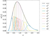 |
Fig. 1 Underlying theoretical distribution of the number density of galaxies n(z) (black dashed line), normalised to one, together with the ni(z) (solid colored lines) at each of the 10 tomographic redshift bins (dotted vertical colored lines), normalised to 1/10. The ni(z) are wide and overlap each other due to the photometric redshift errors. |
Redshift-dependent survey specifications evaluated at the central redshift zi of each redshift bin.
3.1.2 Detailed numerical implementation
The nonlinear matter power spectrum Pm(k, z) is obtained from either CLASS or CAMB. Nonlinear corrections are computed within these codes using Halofit – including Takahashi et al. (2020) and Bird et al. (2012) corrections, see Appendix A.4 for details. The nonlinear power spectrum is approximated as zero outside of the range [kmin, kmax] = [0.001, 50] h Mpc−1. This range is sufficient to include most of the tails of the convolution kernels in Eq. (12) even for the multipoles ℓmin = 10 and ℓmax = 5000. The growth factor D(z) is also extracted from CLASS or CAMB. In the case of MontePython, CLASS is called on-the-fly at every point in cosmological parameter space. On the other hand, CosmicFish can call either CLASS or CAMB on-the-fly, but it also can read a set of pre-computed files with cosmological quantities produced by any arbitrary EBS.
In the case of MontePython, which can also be used to perform MCMCs, computing the matrix elements  for every single ℓ would be numerically expensive. Using the fact that these elements are smooth functions of ℓ, we only compute them on a discrete grid of values of size 100 (with logarithmic spacing between ℓmin and ℓmax) and then use a spline interpolation to get them at every integer ℓ within the range [ℓmin, ℓmax]. The log-likelihood is computed by summing over all integer values of ℓ. In the case of CosmicFish, the angular spectra are computed on the same grid and do not need further interpolation, since the sum is evaluated only over the 100 ℓ-bins.
3.2 Spectroscopic likelihood
3.2.1 General expression
The details of our recipe for the spectroscopic likelihood have been described in many previous papers, including EP:VII. Here we just summarize briefly the set of relations and assumptions used by our CosmicFish and MontePython pipelines, which match the prescription adopted by EP:VII.
For the purpose of evaluating either the likelihood, see Eq. (9), or directly of the Fisher matrix, see Eq. (10), both CosmicFish and MontePython require the calculation of the observed redshift-space galaxy power spectrum Pobs(k, µ, z) at wavenumber k, angle cosine µ, and redshift z. The calculation of this quantity starts from the evaluation of the linear real-space matter power spectrum Pm,lin(k, z), which can be computed with CAMB or CLASS. The calculation sticks to scales where one can assume a linear relation between the galaxy and matter power spectra. Then, the real-space galaxy linear power spectrum reads
 (23)
(23)
where b(z) is the effective galaxy bias. We assume a constant bias bi in each redshift bin i (with central redshift value zi). Bin edges and fiducial bias values are specified in Table 2. To obtain the redshift-space galaxy linear power spectrum, one should further multiply Pm,lin by the Kaiser correction factor (Kaiser 1987)
![Mathematical equation: ${\left[ {b(z) + f(z){\mu ^2}} \right]^2},$](/articles/aa/full_html/2024/02/aa46772-23/aa46772-23-eq72.png) (24)
(24)
where  is the cosine of the angle between the wave-vector k and the line-of-sight direction
  and f(z) is the scale-independent growth rate12. In absence of massive neutrinos (or modified gravity effects), the redshift dependence of σ8(z) can be modeled as
 (25)
(25)
The Fingers-of-God effect can be accounted with an additional prefactor FFoG(z), that we model as a Lorentzian (see e.g. Percival et al. 2004),
![Mathematical equation: ${F_{{\rm{FoG}}}}(z) = {1 \over {1 + {{\left[ {f(z)k\mu \sigma _p^{{\rm{fid}}}(z)} \right]}^2}}},$](/articles/aa/full_html/2024/02/aa46772-23/aa46772-23-eq76.png) (26)
(26)
where the dispersion  is given by an integral over the linear spectrum of the fiducial model,
![Mathematical equation: ${\left[ {\sigma _p^{{\rm{fid}}}(z)} \right]^2} = {1 \over {6{\pi ^2}}}\mathop \smallint \nolimits^ {\rm{d}}kP_{{\rm{m}},{\rm{lin}}}^{{\rm{fid}}}(k,z).$](/articles/aa/full_html/2024/02/aa46772-23/aa46772-23-eq78.png) (27)
(27)
In practice, for the latter integral, we use finite boundaries specified in the next section.
Furthermore, baryon acoustic oscillations in the power spectrum are smoothed out by nonlinear matter clustering. This effect can be approximately modelled by replacing Pm,lin with the de-wiggled power spectrum
 (28)
(28)
![Mathematical equation: ${{g_\mu }(k,\mu ,z) = {{\left[ {\sigma _\upsilon ^{{\rm{fid}}}(z)} \right]}^2}\left\{ {1 - {\mu ^2} + {\mu ^2}{{\left[ {1 + {f^{{\rm{fid}}}}(z)} \right]}^2}} \right\},}$](/articles/aa/full_html/2024/02/aa46772-23/aa46772-23-eq80.png) (29)
(29)
where in this case ffid(z) is fixed to the fiducial cosmology. The no-wiggle power spectrum Pnw(k, z) is obtained by smoothing Pm,lin(k, z) as described in the next section. The variance of the displacement field ![Mathematical equation: ${\left[ {\sigma _\upsilon ^{{\rm{fid}}}} \right]^2}$](/articles/aa/full_html/2024/02/aa46772-23/aa46772-23-eq81.png) for the fiducial model is set equal to the quantity
for the fiducial model is set equal to the quantity ![Mathematical equation: ${\left[ {\sigma _p^{{\rm{fid}}}} \right]^2}$](/articles/aa/full_html/2024/02/aa46772-23/aa46772-23-eq82.png) defined in Eq. (27).
defined in Eq. (27).
In EP:VII, two cases were considered. In the first one, συ and σp were treated as free parameters in each redshift bin, with fiducial values calculated at the zmean of the survey and rescaled by the growth factor D(z). These parameters were then marginalized over. In the second one, in each redshift bin, these parameters were fixed to their fiducial value (computed with the power spectrum of the fiducial cosmology). The latter case assumes a better knowledge of nonlinear corrections and leads to more optimistic constraints. In this paper, we have stuck to the second option and kept these variables fixed in both our pessimistic and optimistic approaches.
Additionally, spectroscopic redshift errors further suppress this power spectrum by an overall factor
![Mathematical equation: ${F_z}(k,\mu ,z) = \exp \left[ { - {k^2}{\mu ^2}\sigma _r^2(z)} \right],$](/articles/aa/full_html/2024/02/aa46772-23/aa46772-23-eq83.png) (30)
(30)
where σr(z) is the comoving distance error, which depends on the linear scaling of the redshift error σ0,z:
 (31)
(31)
The value of σ0,z is given in Table 3.
Next, the Alcock-Paczyński effect introduces a change of the observed wavenumbers and angles with respect to the reference cosmology used for the analysis (identified here to the fiducial model). In particular, distances parallel to the line of sight and orthogonal to it are modified respectively by
 (32)
(32)
where
 (33)
(33)
Then, using  and µ = k‖/k for both the fiducial wavevector (with no subscript) and the observed one (with subscript ‘obs’), we can express the observed wavevector components as a function of the fiducial ones,
![Mathematical equation: ${k_{{\rm{obs}}}} = k{q_ \bot }{h \over {{h^{{\rm{fid}}}}}}{\left[ {1 + {\mu ^2}\left( {{{q_\parallel ^2} \over {q_ \bot ^2}} - 1} \right)} \right]^{1/2}},$](/articles/aa/full_html/2024/02/aa46772-23/aa46772-23-eq88.png) (34)
(34)
![Mathematical equation: ${\mu _{{\rm{obs}}}} = \mu {{{q_\parallel }} \over {{q_ \bot }}}{\left[ {1 + {\mu ^2}\left( {{{q_\parallel ^2} \over {q_ \bot ^2}} - 1} \right)} \right]^{ - 1/2}}.$](/articles/aa/full_html/2024/02/aa46772-23/aa46772-23-eq89.png) (35)
(35)
This shows explicitly that µobs is a function of (µ, z) while kobs is a function of (k, µ, z). Additionally, the Alcock-Paczyński effect implies that the overall power spectrum is multiplied by a factor of  .
.
Finally, we also include a shot noise parameter Ps(z):
 (36)
(36)
where the residual shot noise ps(zi) is treated as a nuisance parameter with a fiducial value of 0 in each redshift bin, and  is the galaxy number density in each bin given in Table 2. In summary, the observed galaxy power spectrum in each bin reads (EP:VII)
![Mathematical equation: $\eqalign{ & {P_{{\rm{obs}}}}\left( {{k_{{\rm{obs}}}},{\mu _{{\rm{obs}}}},{z_i}} \right) = q_ \bot ^2{q_} \cr & & & \times {{{{\left[ {{b_i}{\sigma _8}\left( {{z_i}} \right) + f\left( {{z_i}} \right){\sigma _8}\left( {{z_i}} \right)\mu _{{\rm{obs}}}^2} \right]}^2}} \over {1 + {{\left[ {{f^{{\rm{fid}}}}\left( {{z_i}} \right){k_{{\rm{obs}}}}{\mu _{{\rm{obs}}}}\sigma _p^{{\rm{fid}}}\left( {{z_i}} \right)} \right]}^2}}} \cr & & & \times {{{P_{{\rm{dw}}}}\left( {{k_{{\rm{obs}}}},{\mu _{{\rm{obs}}}},{z_i}} \right)} \over {\sigma _8^2\left( {{z_i}} \right)}}{F_z}\left( {{k_{{\rm{obs}}}},{\mu _{{\rm{obs}}}},{z_i}} \right) \cr & & & + {P_{\rm{s}}}\left( {{z_i}} \right), \cr} $](/articles/aa/full_html/2024/02/aa46772-23/aa46772-23-eq93.png) (37)
(37)
where we omitted the arguments of the functions kobs(k, µ, z) and µobs(µ, z). In each redshift bin the product biσ8(zi) is actually treated as an independent nuisance parameter, which means that it is kept fixed when varying the cosmological parameter σ8. Together with the values of ps(zi) the spectroscopic case features a total of 8 nuisance parameters. The fiducial value of each biσ8(zi) is inferred from the  value reported in Table 2 multiplied by
  (see Table B.2 for exact values).
To evaluate the likelihood (resp. the Fisher matrix), one should insert this expression into Eq. (9) (resp. into Eq. 10), which also depends on the volume  in each bin, whose values are listed in Table 2. Finally, one should integrate over k from kmin to kmax (whose values are given in Table 3 for the pessimistic and an optimistic case) and µ from −1 to +1.
Specifications used in the spectroscopic likelihood and Fisher formulas.
3.2.2 Detailed numerical implementation
For the sake of reproducibility, we provide here some details on the discretisation schemes, interpolation routines and integration algorithms used in our CosmicFish and MontePython pipelines. These settings ensure some well-converged calculations, such that changing them slightly would have a negligible impact on our results.
In our CosmicFish or MontePython algorithms the linear matter power spectrum Pm,lin(k, z) is returned by CAMB or CLASS on a logarithmically-spaced grid of 1055 discrete values of k ranging from kmin = 3.528 × 10⁻⁵ Mpc−1 to kmax = 50.79 Mpc−1, corresponding to a logarithmic stepsize of d ln k = 0.01354.
The value of σ8(z = 0) is read from CAMB or CLASS. The growth factor D(z) and growth rate f(z) are also extracted from CAMB or CLASS. Then σ8(zi) is approximated as σ8(0) D(zi)/D(0).
The no-wiggle power spectrum Pnw(k, z) is inferred from Pmin(k, z) using a Savitzky-Golay filter of order 3 on the same grid of 1055 points evenly spaced in (ln k) (see e.g. Boyle & Komatsu 2018). The filter’s window length is set to 101 points, which corresponds to a smoothing over Δ ln k = 100 ln(1 + dln k) = 1.359.
The algorithm then builds interpolators for Pmin(k, z) and Pnw(k, z) (using the scipy CubicSpline algorithm in MontePython and the order-3 RectBivariate spline algorithm in CosmicFish). The final likelihood requires the evaluation of several quantities – including these two spectra – on a three-dimensional grid (ki, µj, zk), or, in the case of theoretical power spectra, (kobs,i, µobs,j, zk) = [kobs(ki, µj, zk), µobs(µj, zk), zk]. In this grid, for MontePython (CosmicFish), ki takes 500 (2048) discrete values of k between some kmin and kmax (whose values are reported in Table 3) with even logarithmic spacing, additionally µj takes 9 (128) discrete values evenly spaced between −1 and +1. Finally, zk runs over the 4 central redshift values of the 4 redshift bins reported in Table 3.
We have tested that having only 9 values for the grid in µ is enough for our purposes in both MontePython and CosmicFish when the integral is performed using the Simpson algorithm of the Python package scipy (Virtanen et al. 2020). However, for CosmicFish we kept the grid of 128 values in µ, since in general it is a much more time-efficient code. In both codes the final integral over k is also performed using the Simpson algorithm.
4 Validation of the forecast pipelines
4.1 Methodology
In this work, for each survey and each settings, we have compared five Fisher matrices corresponding to the following five cases:
CF/ext/CAMB: With this method, CosmicFish (CF) reads the information (spectra, distances…) in files produced in advance (externally) by CAMB. This is one of the methods used in EP:VII. Thus, we include this case in order to cross-check that nothing significant has changed within the CosmicFish code such that, a couple of years later, it still agrees with the results of EP:VII.
CF/int/CAMB: CosmicFish calls CAMB internally to extract all relevant information (spectra, distances…) on the fly: this is a more efficient approach that we also want to validate here. The comparison with the first case has proven that we integrated CAMB within CosmicFish in a correct way, with a proper use of the CAMB Python wrapper.
CF/ext/CLASS: CosmicFish reads the relevant information in files similar to those of the first method, but produced in advance by CLASS. The comparison of this method with the first one has proven that the theoretical predictions from CAMB and CLASS agree within the sensitivity of Euclid.
CF/int/CLASS: CosmicFish calls CLASS internally to extract all relevant information on the fly: this is again a more efficient approach than the external one. The comparison with the third case is a proof that we integrated CLASS within CosmicFish in a correct way, with a proper use of the CLASS Python wrapper.
MP/Fisher: MontePython (MP) runs in Fisher mode and extracts all cosmological information on the fly from CLASS. The primary goal of this paper is to validate this pipeline against that of EP:VII.
We have treated our results for the CF/ext/CAMB case as the “reference result” corresponding to the recipes of EP:VII. In order to show that this choice is justified, we have also directly compared the above five Fisher matrices with a second reference Fisher matrix from EP:VII. In the photometric case our second reference was the Fisher matrix posted on the online repository fisher_for_public9. In the spectroscopic case the second reference was be provided by SoapFish (SF), which is another of the codes validated by the EP:VII group. Similar to CF/ext/CAMB, the SF pipeline relies on external files produced by CAMB.
Finally, we can also estimate the survey sensitivity to cosmological parameter using the MP/MCMC method, that is, fitting some fiducial Euclid data with our Euclid mock likelihoods (which are the very same likelihoods as in the MP/Fisher method), while exploring the parameter space with MCMCs. The focus of this paper is not on the comparison between Fisher and MCMC results. Still, knowing the MCMC results is useful in order to cross-check our Fisher results, evaluate the level of Gaussianity of our likelihood with respect to model parameters, or get insight on parameter degeneracies.
In the following section, we have compared the results given by all these methods with a seven-parameter cosmology (ΛCDM+{w0, wa}). Fiducial values of cosmological and nuisance parameters are summarised in Table B.1. We have proven that all our Fisher pipelines agree with each other within at most 10%, which is the validation threshold set by the EP:VII publication.
Since for each case (photometric/spectroscopic survey with pessimistic/optimistic settings) we have five ways to compute the Fisher matrix, we can perform ten comparisons between pairs of matrices. The comparison can be made at the level of unmarginalised or marginalised errors. Unmarginalised errors correspond to the error on one parameter when all other parameters are kept fixed. This only involves the diagonal coefficients of the Fisher matrices. Marginalised errors instead represent the error on one parameter when all the others are unknown (and only constrained by the experiment). This involves the diagonal coefficients of the inverse Fisher matrices. As such, it depends on all coefficients in the Fisher matrices, or in other words, on the Fisher estimate of correlations between all pairs of parameters.
The most important quantities which we use for validation are of course the marginalised errors. Still, the knowledge of the unmarginalised ones is often useful. We have reported on both in what follows.
4.2 Photometric likelihood
4.2.1 Pessimistic setting
Table 4 contains the most relevant information for the photometric survey with pessimistic settings, that is, the biggest discrepancy between marginalised errors computed across all cosmological and nuisance parameters in each of the 10 comparisons that can be made. The result is presented as a five-by-five symmetric matrix (with no information along the diagonal since each method agrees with itself). In a nutshell, since the worst difference is at the level of 2% and thus well below the 10% threshold set in the EP:VII publication, all five methods are validated – that is, are in sufficiently good agreement with EP:VII results. We provide a more detailed discussion below.
To begin, we observe that the two methods that use CosmicFish combined with CAMB are highly consistent with each other. The largest difference across all errors is only of 1.2%. Individual marginalised and unmarginalised errors for these two cases are compared in Fig. 2 (first panel). In such plots, sticking to the plotting conventions of previous papers such as EP:VII, we show the percentage discrepancy of each marginalised or unmarginalised error σi with respect to the median13. This comparison proves that the integration of CAMB within CosmicFish has been done consistently. Note that CF/ext/CAMB uses only the CAMB Fortran code, while CF/int/CAMB uses also the CAMB Python wrapper to extract quantities. The order 1% differences found here can be attributed to details in the numerical algorithms used within this Python wrapper or within CosmicFish, or different ways to interpret precision parameters in the CAMB Fortran code and Python wrapper, see Sect. 6 for details on accuracy settings. These differences are anyway hardly relevant and do not deserve further attention.
The two methods using CosmicFish combined with CLASS are even more consistent, with a worst error of 0.02%. Individual marginalised and unmarginalised errors for these two cases are compared in Fig. 2 (second panel). This proves that the integration of CLASS within CosmicFish has also been done correctly. In the CLASS case, there is less room for differences, because the Python wrapper c1assy is used by both the external and internal methods14.
At this point, we know that using CosmicFish in external or internal mode makes no difference, and we can investigate the level of consistency of the CAMB and CLASS predictions. Comparing for instance the CF/int/CAMB and CF/int/CLASS methods, we find again excellent agreement, with a worst error of 0.10%. All individual marginalised and unmarginalised errors for these two cases are compared in Fig. 2 (third panel). Other comparisons between the CAMB-based and CLASS-based methods are nearly as good, as can be checked from Table 4. This shows that using CAMB or CLASS as our theory code makes no difference at the level of sensitivity of Euclid. Note that, in order to reach such a conclusion, we had to enhance the settings of a few accuracy parameters in the two codes and to ensure a very good match of the physical assumptions that they use, for example on the neutrino sector. These precise settings are detailed in Appendix A and commented in Sect. 6. We recommend using at least the precision settings discussed in Sect. 6 in any forecast or real data analysis for Euclid or experiments with comparable sensitivity.
At this stage, we have validated all the methods involving CosmicFish. We are only left with the comparison of the CosmicFish versus MP/Fisher results.
We see in Table 4 and in the fourth panel of Fig. 2 that the worst discrepancy between the CosmicFish and MontePython pipelines reaches about 2.0%. Since this is much lower than the validation threshold, the MontePython Fisher pipeline is validated. We even performed a more demanding test: We compared all the pipelines presented in this paper to the final average results of EP:VII, available in the public repository fisher_for_public9. Figure 3 shows a final comparison between the Fisher marginalised and unmarginalised error from CosmicFish, MontePython, and EP:VII. We find a maximum deviation with respect to the mean of 5%, which confirms validation. Note that CosmicFish results are already known to agree with the results of EP:VII, since an older Fortran-based version of this code was one of the codes employed for the code-comparison project of EP:VII. However, these last tests demonstrates that the CosmicFish pipeline used in this work is fully consistent with the older CosmicFish implementation.
Moreover, the visual comparison of Fisher ellipses with MCMC confidence contours presented in Fig. 4 for cosmological parameters (and in Figs. C.1 and C.2 for nuisance parameters) is enlightening. The MCMC contours turn out to be almost perfectly elliptical for all parameters. Thus, the approximation of a multivariate Gaussian likelihood, assumed in the Fisher method, is a good one. In all cases, the MCMC contours remain very close to the Fisher ellipses. This excludes the possibility that our Fisher results agree with each other accidentally, while being far from the actual confidence limits associated to the full likelihoods. It also confirms that, for each one of our Fisher methods, the numerical derivative step sizes have been chosen in a sensible way, that is, large enough to overcome numerical noise and small enough to remain in the region where the likelihood is approximately Gaussian (see Appendices B.2 and B.3 for details).
For the photometric survey with pessimistic settings, and for each pair of Fisher matrices obtained with different methods, largest percentage difference between the predicted marginalised error on each parameter (across all cosmological and nuisance parameters).
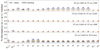 |
Fig. 2 For the photometric survey with pessimistic settings, and for selected pair of Fisher matrices obtained with different methods, comparison of each Fisher marginalised (blue dot/light grey) and unmarginalised (orange dot/dark grey) error on each cosmological and nuisance parameters, for: (First) CF/ext/CAMB versus CF/int/CAMB; (Second) CF/ext/CLASS versus CF/int/CLASS; (Third) CF/int/CLASS versus CF/int/CAMB; (Fourth) CF/int/CLASS versus MP/Fisher. Each forecasted error σi for each case and parameter is compared to the median of the two cases (see footnote 13). The discrepancy is expressed in percent. |
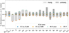 |
Fig. 3 For the photometric survey with pessimistic settings, comparison of each Fisher marginalised (light grey) and unmarginalised (dark grey) errors on the cosmological and nuisance parameters, for: CF/int/CLASS (blue circles) versus CF/int/CAMB (orange squares) versus MP/Fisher (green stars) versus the public EP:VII results (red crosses, referred in the legend as IST:F). Each forecasted error σi for each case and parameter is compared to the median of the four cases, and the discrepancy is expressed in percent. |
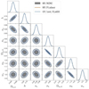 |
Fig. 4 For the photometric survey with pessimistic settings, comparison of 1D posteriors and 2D contours (for 68 and 95% confidence level) from different methods: MP/MCMC (grey lines/contours), MP/Fisher (orange lines), CF/int/CLASS (blue lines). We only show here the cos-mological parameters, but our contours involving nuisance parameters are shown in Appendix C. Plotted using GetDist. |
4.2.2 Optimistic setting
In this case, our results are summarised in Table 5 and Fig. 5. Qualitatively, all the conclusions reached for the pessimistic case also apply to this case.
A priori, with optimistic settings, we may expect larger differences between our four CosmicFish pipelines, because the likelihood is more sensitive to theoretical predictions for the nonlinear matter power spectrum. Indeed, the optimistic likelihood probes a larger range of k values in the nonlinear power spectrum and has smaller observational errors. Thus, numerical errors are less likely to be masked by observational errors. However, we find that the differences between the four CosmicFish pipelines (with internal/external CAMB/CLASS) increase only marginally. For instance, CF/int/CAMB and CF/int/CLASS still agree at an impressive 0.55% level (instead of 0.11% with pessimistic settings). The agreement between CF/int/CAMB and CF/ext/CAMB is a bit worse (1.3%), showing that the CAMB Fortran code and the CAMB Python wrapper handle accuracy settings differently, with a small but noticeable impact on small-scale predictions for the nonlinear power spectrum. The better agreement of the CF/int/CAMB pipeline with the CLASS pipeline suggests that CAMB is more accurate when called through the Python wrapper – consistent with the fact that this implementation is the most recent one15.
Besides, differences between CosmicFish and MontePython also increase with respect to the pessimistic case, but only to the level of 4.3%. Figure 5 (bottom plot) shows that the difference is now dominated by the marginalised error on (w0, wa), that is, by the calculation of correlations between dark energy parameters and other parameters. However, the 10% validation threshold is fulfilled. Even when we include the official EP:VII results in the comparison, as in Fig. 6, the (un)marginalised errors differ from the median by at most 9%.
In conclusion, our pipelines are also all validated in the photometric optimistic case. As a final check, the comparison between MCMC contours and Fisher ellipses in Fig. 7 brings a final confirmation of the robustness of our forecasts against possible issues related to numerical noise or non-Gaussian posteriors (Fig. 7 only includes cosmological parameters, but the plots for nuisance parameters are available in our public repository16).
4.3 Spectroscopic likelihood
4.3.1 Pessimistic setting
In this case, our results are summarised in Table 6 and Fig. 8. Qualitatively, there are no big differences between the conclusions to be drawn from the photometric and spectroscopic surveys.
As a matter of fact, the two pipelines using CosmicFish combined with CAMB are consistent with each other, with small differences in the errors of at most 2.1% – caused again by differences in the treatment of accuracy between the Fortran and Python methods for calling CAMB. Once more, the pipelines using CosmicFish combined with CLASS are even more consistent, with a largest differences of 0.12%. When CosmicFi sh switches from the CF/int/CAMB method to the CF/int/CLASS method, the errors remain unchanged up to 0.26% differences.
The MP/Fisher pipeline gets validated in the spectro-scopic/optimistic case, with differences of at most 2.9% with respect to CF/ext/CAMB and 1.4% with respect to the other CosmicFish methods. This was comparable to our results for the photometric probe. Our pipelines also passed successfully a more demanding test: when we add to the comparison set some previous EP:VII results, all errors remain within 5% of the median, as shown in Fig. 9. In this case, previous EP:VII results are represented by those of the SOAPFish code, as already mentioned in Sect. 4.1.
Our Fisher forecasts agree very well not only among each other, but also with the MCMC forecast shown for comparison in Fig. 10 for cosmological parameters (and Figs. C.3 and C.4 for nuisance parameters). Here, we can see by eye a small level of non-Gaussianity in the 1D and 2D posteriors. However, the Fisher ellipses appear to be excellent approximations to the actual confidence contours.
In a previously published work by Yahia-Cherif et al. (2021), the emphasis was placed on validating only the spectroscopic likelihood for stage-IV surveys. The authors conducted a thorough evaluation of various numerical derivative methods, assessing their impact on the stability of the Fisher matrix. Additionally, they compared the results of their analysis with those obtained through MCMC runs. Our findings align with those of Yahia-Cherif et al. (2021), demonstrating a comparable level of agreement.
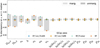 |
Fig. 9 For the spectroscopic survey with pessimistic settings, comparison of each Fisher marginalised (light grey) and unmarginalised (dark grey) errors on the cosmological and nuisance parameters, for the cases of: CF/int/CLASS (blue circles) versus CF/int/CAMB (orange squares) versus MP/Fisher (green stars) versus EP:VII results from SOAPFish (SF, red crosses). Plotting conventions are the same as in Fig. 3. |
4.3.2 Optimistic setting
This last case is very similar to the previous one. Switching to optimistic settings in the spectroscopic likelihood does not degrade nor improve significantly the comparison between the various approaches as can be seen by comparing Fig. 8 to Fig. 11. The difference between all marginalised CosmicFish and MontePython Fisher errors is below the 2.5% level, see Table 7. When adding SOAPFish to the comparison set, the difference increases to 6%, see Fig. 12, still small enough to validate our MP/Fisher pipeline. The very good agreement between all Fisher forecasts and an MP/MCMC forecast is shown for comparison in Fig. 13 for cosmological parameters (and in the repository17 for nuisance parameters).
5 Forecast results
5.1 Photometric survey alone
In Tables 8 and 9 we show the absolute 1σ errors on each cosmological parameters obtained for the photometric probe with our CosmicFish, MP/Fisher, and MP/MCMC pipelines. We compare them with the mean values obtained by EP:VII. For CosmicFish, we take here numbers from the CF/int/CLASS case – but we know from previous sections that other cases give essentially the same results.
Previous tables showed the largest percentage difference between error bars across all cosmological and nuisance parameters. Here, by comparing different columns, one can check for individual parameters that these percentage differences are always very small – even if the error bars of EP:VII are usually more optimistic than other errors by a tiny amount.
For the photometric survey with pessimistic settings, marginalised 1σ errors on cosmological parameters found by: the average of EP:VII results, CF/int/CLASS (the other versions of CosmicFish give nearly the same results), MontePython in Fisher mode, MontePython in MCMC mode.
5.2 Spectroscopic survey alone
In Tables 10 and 11 we show the absolute 1σ errors on each cosmological parameters obtained with the same pipelines, but now for the spectroscopic probe. Note that there is a minor difference between our implementation and the EP:VII one regarding the nonlinear modelling. As a matter of fact, our pessimistic and optimistic cases agree in the kmax used for the probes, namely 0.25h Mpc−1 and 0.30h Mpc−1, respectively. However, the pessimistic case of EP:VII is more conservative, since it marginalizes over the nonlinear parameters σp and συ, while here we keep them both fixed at the fiducial cosmology, as already explained in Sect. 3.2. Moreover, the recipe of EP:VII assumes a separation into shape- and redshift-dependent parameters for the observed galaxy power spectrum. In that recipe, the redshift-dependent parameters – which are H(𝓏i), dA(𝓏i), f σ8(𝓏i) and bσ8(𝓏i) – are varied freely at each redshift bin and then projected onto the final cosmological parameter basis (or marginalized over in the case of the galaxy bias). This is again more conservative, firstly, because it assumes more freedom in the modelling of the observables, and secondly, because the marginalization over a larger parameter space degrades the constraints. Since EP:VII did not publish a Fisher matrix using our direct full-shape method approach, we compare against the code SoapFish, which does contain the same implementation and is one of the validated codes of the EP:VII group.
For the combined photometric and spectroscopic surveys with various combinations of pessimistic and optimistic settings, marginalised 1σ errors on cosmological parameters found by CF/int/CLASS (the other versions of CosmicFish give nearly the same results).
5.3 Combined surveys
We finally combine the photometric and spectroscopic probes, which amounts in summing up their Fisher matrices. We consider all four combinations of pessimistic or optimistic settings for each probe. The absolute 1σ errors on each cosmological parameters obtained with CosmicFish are shown in Table 12. We take here numbers from the CF/int/CLASS case – but we cross-checked that other cases give essentially the same numbers. To visualise the way in which the combined probe lifts parameter degeneracies, the best is to compare the Fisher ellipses coming from individual and combined probes. These are shown in Fig. 14 for the optimistic-optimistic case, in Appendix D for the pessimistic-pessimistic case, and in our repository for other cases18.
Note that, in principle, there is a correlation between data from the photometric and spectroscopic galaxy clustering probes at the redshifts where they overlap. In this section, we neglect this correlation for simplicity, which makes our forecasts slightly too optimistic. This differs from the ‘EP:VII pessimistic’ approach, in which high-redshift data were removed from the photometric survey, leading instead to slightly too pessimistic results.
The combination is particularly efficient for the determination of Ωb,0 and h, for which the photometric and spectroscopic surveys probe different degeneracy directions. The combination reduces significantly the error on these parameters compared to each individual probe. For other parameters the measurement is dominated by the photometric probe.
A traditional estimate of the constraining power of a survey dedicated to the study of dark energy is the dark energy Figure of Merit (DE FoM), which is defined as
 (38)
(38)
where  is the 2 × 2 Fisher matrix after marginalizing over all other cosmological and nuisance parameters except w0 and Wa. For a Gaussian posterior (i.e. for elliptical Fisher contours) this quantity is related to the area S of the 1σ probability contours by
 (39)
(39)
For a Fisher matrix the computation of the determinant is a trivial operation, while for MCMC chains there are two options. The first option, and most common in the literature, is to compute the covariance matrix of the chains, which is a good approximation if the posterior is Gaussian: then, the covariance matrix is equivalent to the inverse of the Fisher matrix. However, since the covariance matrix is by definition symmetrical, computing the DE FoM from it might under- or over-estimate the constraining power of the probe in the w0-wa parameter space. The difference would depend on the exact shape of the MCMC contours and how non-Gaussian they are. The second option is to use Eq. (39) to calculate the FoM from the enclosed area of the MCMC contour itself. The computation of such contours is a well-known problem in the literature. The reader can refer to Lewis (2019) and Brinckmann & Lesgourgues (2019) for more details on the estimation of the probability contours from a discrete set of Markov chains.
For the photometric probe, since our approach is exactly equivalent to the one of EP:VII, we also find exactly the same DE FoM. For the spectroscopic one, we have highlighted and proved in this work that, while using the same likelihood recipe, we adopt a different parametrisation: we directly compute the Fisher matrix in the space of cosmological parameters, while EP:VII computed it with respect to a basis of phenomenological parameters and then used a non-trivial transformation to go to the space of cosmological parameters. Thus we find a slightly different FoM, that we provide for completeness in Table 13 -using either one of the CosmicFish Fisher pipelines or the MCMC pipeline with an evaluation of the area enclosed by the marginalised contours.
6 Impact of accuracy settings in Einstein-Boltzmann solvers
CAMB and CLASS have been proved to agree remarkably well with each other when using very high accuracy settings (see Lesgourgues 2011b). The settings defined in Lesgourgues (2011b) are however unpractical because they slow down both codes considerably. The question of properly choosing the default value of each precision parameter in CAMB and CLASS has been extensively investigated and tested by various groups from 2011 to 2013, that is, during the first stages of the Planck data analysis (see Hamann et al. 2009; Lesgourgues 2011b; Lesgourgues & Tram 2014). Since then, both codes are provided with default-precision settings designed to avoid biasing the results of MCMC analyses of, typically, Planck and SDSS/BOSS data, while keeping them as fast as possible.
Accuracy settings in CAMB and CLASS deserve to be revisited in the present context, mainly for three reasons. First, in general, Fisher analyses require more precision than MCMC runs. Indeed, the calculation of numerical derivatives involves the comparison of power spectra obtained under very small variations of cosmological parameters. These variations should be dominated by physical effects rather than numerical errors. MCMC runs avoid such an issue because, in MCMCs random numerical errors tend to be averaged out each time that results are marginalised over unwanted parameters. Thus, in this work, MCMC runs are always performed with default CLASS precision. Second, among the Fisher methods used here, the MP/Fisher method, which requires the calculation of second derivatives of the likelihood, tends to require even higher precision. Third, Euclid probes the matter power spectrum with much higher accuracy than SDSS/BOSS. Precision parameters that are particularly relevant for computing the matter power spectrum need to be tuned accordingly.
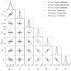 |
Fig. 14 For the individual and combined photometric and spectroscopic surveys with optimistic settings, 1D posterior and 2D contours (for 68% and 95% confidence level) on cosmological parameters from CF/int/CLASS (dotted lines) and MP/Fisher (solid lines). Plotted using GetDist. |
Dark energy Figure of Merit for the spectroscopic survey with optimistic and pessimistic settings, found by: the determinant of the CosmicFish Fisher matrix and the area of the MontePython MCMC contours.
6.1 Accuracy settings and fiducial spectra
In Appendix A we detail the list of all fixed parameters passed to CAMB and CLASS before each run. The list includes a few options concerning the setting of key precision parameters. Here we summarise these different settings and we show how they impact the accuracy of the power spectrum calculation for a given cosmological model – in this section we just chose to focus on the fiducial model19. For more details the reader can consult Appendix A.
For CAMB the two parameters accuracy_boost and l_accuracy_boost play an essential role for the calculation of background, thermodynamical, and perturbation quantities for each cosmology. In this work, we never consider values of these parameters below 2 (2 was the setting adopted in EP:VII). Additionally, in the context of Fisher forecasts one must be aware of the role of a tolerance parameter in the version of Halofit implemented in CAMB. This tolerance governs the accuracy with which the algorithm finds the scale of nonlinearity for each cosmology, using a bisection method. In CAMBthis tolerance is hard-coded to 10−3. We replaced it by a new accuracy parameter passed in input, halofit_tol_sigma, and we explored values down to 10−6 (we checked that even smaller values make no difference within CosmicFish forecasts). We define three precision settings for CAMB, which we call P1, P2, P3 in order of growing precision: CAMB (P1 /P2/P3)
accuracy_boost =2/2/3
l_accuracy_boost =2/2/3
halofit_tol_sigma = 1.e-3 / 1.e–6 / 1.e–6
Thus, (P1) corresponds to settings of EP:VII, (P2) shows the impact of decreasing the Halofit tolerance by 3 orders of magnitude, and (P3) stands for our most enhanced settings, used by default in the rest of this work.
For CLASSwe considered the default-precision (DP) settings of the public code and compare them with high-precision (HP) settings. In order to define the latter, we recall that CLASS is downloaded together with an optional input file called pk_ref.pre, designed to push the code to extreme accuracy, and used in Lesgourgues (2011b) to demonstrate that boosted versions of CAMB and CLASS do agree at the 0.01% level for the matter power spectrum and other observables. These settings are unpractical for forecasting purposes due to their CPU cost. Additionally, many parameters in pk_ref.pre are irrelevant for the calculation of the matter power spectrum. In Appendix A.5 we propose a more concise set of accuracy parameters that define our HP settings. We have shown here that these HP settings lead to a very good convergence of the matter power spectrum without slowing CLASS down in an exaggerated way. The tolerance parameter of Halofit is set by default to 10−6 within CLASS (as well as in our CAMB P2 and P3 settings). We lower it to 10−8 in CLASS HP settings (this is lower than in CAMB P2 and P3, because CLASS is used within the MP/Fisher pipeline which, as argued before, requires extra precision).
In Fig. 15 we compare the linear and nonlinear spectrum of the fiducial model at redshift z = 0 and z = 2, computed with each version of CAMB and CLASS. Here, CLASS HP is always used as a reference.
First, we can compare the results with the highest settings: in Fig. 15 the red curves show the ratio of the CAMB P3 over CLASS HP spectra. We see that the relative difference is always below 0.07% for the linear spectrum. This is not as small as the 0.01% agreement found in Lesgourgues (2011b), because this reference relied on even higher precision settings, with accuracy boost parameters as large as (4, 8) in CAMBand settings from pk_ref.pre in CLASS. Nevertheless, a 0.07% agreement is remarkable and definitely sufficient for the purpose of our forecasts, as demonstrated by the agreement between the various Fisher matrices derived in the previous sections. For the nonlinear power spectrum the level of agreement is similar (excepted for a narrow spike of 0.2% at k ⋍ 3.3 × 10⁻³ Mpc−1 coming from the transition from linear to nonlinear calculations in both codes – but a feature at such a low values of k is harmless for Euclid predictions).
Next, we can investigate the impact of degrading precision in the two codes. With CLASS DP the error remains below the 0.1% level on large scales, but slightly exceeds 0.12% on small scales for the linear power spectrum. This is anyhow a very small degradation compared to the sensitivity of Euclid. As a matter of fact, we only observe very small differences between the CosmicFish results obtained with either CLASS DP or HP. However, the HP settings provide more stability against the choice of step sizes when computing the second derivatives of the likelihood with the MP/Fisher approach, as shown in Appendix B.3. Thus, in the rest of this work, we decided to stick everywhere to CLASS HP settings.
Comparing the results from CAMB P2 and P3 in Fig. 15, we see that CAMB P2 is a bit further away from CLASS HP than CAMB P3 on small scales, but this is rather unimportant. The results for P1 and P2 are identical at the level of the linear spectra, since these settings only differ at the level of one Halofit parameter. However, the nonlinear spectra from P1 and P2 differ significantly – at the 0.25% for our fiducial model. This shows that a Halofit tolerance of 10−3 is insufficient. It leads to a poorly converged bisection in Halofit, and thus to a spurious step-like response of the nonlinear spectrum to small variations in the cosmological parameters. Thus, it compromises the calculation of numerical derivatives. We believe that the EP:VII group overcame this difficulty by using advanced methods for the calculation of derivatives, based on multiple steps. With simple two-sided derivatives, it would be nearly impossible to obtain stable derivatives with P1 settings, as we shall see better in the next subsection.
As a small technical detail, we note that in order to produce Fig. 15 we adjusted two parameters in a slightly different way than in the rest of this paper. Instead of passing the same value of σ8 to both codes, we passed the same value of As in order to be insensitive to very small differences in the σ8-to-As conversion performed inside CAMB or CLASS. This choice is relevant only for the sake of producing Fig. 15. Indeed, in the rest of this work we only want to compute the variation of the spectra in the vicinity of the fiducial model. Thus, a very small difference in the absolute value of one cosmological parameter (As) is irrelevant. Therefore, in other sections we can safely adopt the same input value of σ8 in the two codes. In order to match the scale k* at which both codes start computing nonlinear corrections to the power spectrum, we adjusted manually the transition scale parameter in CLASS to its CAMB value, that is, halofit_min_k_nonlinear=3.3e−3. Otherwise, nonlinear corrections are computed by CLASS for any  Mpc−1 and by CAMB for any
  Mpc−1. This produces a small degradation of the CAMB-CLASS agreement for
  . However, Euclid does not probe accurately such huge scales or tiny wavenumbers. Thus, in other parts of this work, we stick to the default value of the CLASS parameter halofit_min_k_nonlinear.
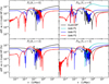 |
Fig. 15 For the linear (left) and nonlinear (right) matter power spectrum of the fiducial model at redshift z = 0 (top) and z = 2 (bottom), percentage difference between the predictions of CLASS and CAMB. Here, the reference is the CLASS high-precision (HP) result. We compare it with CLASS Default Precision (DP) and CAMB with the precision settings defined as P1, P2, P3 in the text. In the linear case (left), the CAMB P1 curve is always overdrawn by the P2 one, since the difference between P1 and P2 is only relevant at the level of the nonlinear spectrum. |
6.2 Accuracy settings and first derivatives of the spectra
We now bring our precision tests to the level of first derivative calculations. Since we use the Limber approximation for the photometric probe, the quantities of interest for both probes are the derivatives of the matter power spectrum. We have shown here the derivatives ∂α In P(k, z) of the linear and nonlinear power spectrum at z = 0 for all cosmological parameters α. Like in our CosmicFish runs we use two-sided derivatives with step sizes Δpα set to 1% of fiducial values (or 0.01 in the case of w0 and wa). Figure 16 shows the derivatives ∂α In P(k, z = 0) as a function of k computed with CLASS DP, HP, and CAMB P1, P2, P3. To see better the difference between these curves, we show in Fig. 17 the difference between the derivatives computed with either CLASS DP, CAMB P1, CAMB P2, or CAMB P3 and those computed with CLASS HP.
For the linear power spectrum all codes and all accuracy settings predict derivatives that are visually identical in Figs. 16 and 17 reveals tiny differences. By comparing the two figures, we see that differences are typically two order of magnitude smaller than the derivative themselves (the biggest discrepancy is a 5% difference between the CAMB and CLASS predictions for the derivative with respect to h). Such a high level of agreement on linear derivatives explains the very good match between the Fisher matrices obtained with CosmicFish/CAMB and CosmicFish/CLASS for the spectro-scopic probe.
At the level of the nonlinear power spectrum, we see in both figures that CAMB P1 predictions are very discrepant - especially for (Ωb, σ8), but also for (Ωm0, h, ns). This is due to the glitches generated by insufficient settings for the Halofit tolerance parameter. However, the level of agreement between CLASS DP, HP and CAMB P2, P3 is again excellent, typically of the same order of magnitude as for the linear spectrum - which proves that Halofit is implemented consistently and accurately in the two codes.
From a glance at Figs. 16 and 17 it is difficult to assess whether the Fisher matrix of the CosmicFish pipeline should be computed with DP or HP for CLASS and with P2 or P3 for CAMB: these settings seem roughly equivalent at the level of these plots. However, tiny differences at the level of derivatives - and thus of Fisher matrices - can be amplified by the Fisher matrix inversion. Thus the only way to check the required level of accuracy is to compare the marginalised errors obtained with different precision levels. We performed such tests using the CF/ext pipeline.
We show the difference between the error inferred from CAMB P2 versus P3 or from from CLASS DP versus HP in Fig. 18. In each test we consider the case of the photometric/optimistic probe (top panels) and spectroscopic/optimistic probe (bottom panels). Here we always use the CF/ext pipeline.
The largest differences appear between CAMB P2 and CAMB P3 for the spectroscopic probe: they are of the order of 1% on marginalised errors. These differences are still small, which suggests that results obtained with P2 are already reasonable, while those of P3 are likely to be well converged. We checked that the results obtained with P3 are the closest ones to the average of other pipelines, and thus, as expected, the most accurate. This motivates our choice to stick to P3 precision in the rest of this work. We recall that the matrices of EP:VII were based on P1 settings and that the significant error introduced by such settings was mitigated through the use of the SteM scheme for the calculation of derivatives.
Between CLASS DP and CLASS HP, we never find differences exceeding 0.5%. Thus, running with HP is not strictly necessary, but it confers extra precision and robustness to the results. In all previous sections, our Fisher matrices were obtained with HP settings.
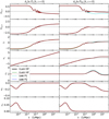 |
Fig. 16 Derivative of the logarithm of the linear (left) and nonlinear (right) matter power spectrum with respect to each cosmological parameter in our basis, computed with CLASS (with either DP or HP) and CAMB (with either P1, P2, or P3 precision). The derivatives are computed at z = 0. In the linear case (left), the CAMB P1 curve is always overdrawn by the P2 one, since the difference between P1 and P2 is only relevant at the level of the nonlinear spectrum. Moreover, P2 is always nearly overdrawn by P3. |
6.3 Accuracy settings and second derivatives of the likelihood
The MP/Fisher pipeline relies on the calculation of second derivatives of the likelihood, which potentially require even more precision than the evaluation of first derivatives. We can do various tests of the impact of accuracy settings on such second derivatives, that is, on the direct calculation of the Fisher matrix coefficient.
In Appendix B.3 we show how the prediction of a given Fisher matrix coefficient varies with the CLASS precision setting (DP versus HP) and the step size. We find that with small step sizes the results can be affected by random numerical noise, while with large step sizes they pick up higher-order contributions related to the non-Gaussianity of the likelihood. Adopting HP settings offers an opportunity to decrease the step sizes without being dominated by numerical noise, and thus, to have a safe and robust calculation of Fisher matrix coefficients, closer to the Gaussian approximation. This supports our decision to stick to HP settings throughout this work – while in the CosmicFish pipeline, based on the calculation of first derivatives, CLASS DP settings would suffice, as shown in the last subsection.
We can also compare the marginalised and unmarginalised errors on all parameters obtained with the MP/Fisher pipeline, using either CLASS DP or HP. For this test, we stick to the same small step sizes as in the rest of this work, that is, for the photometric probe, 10% of the marginalised error on each parameter, and for the spectroscopic probe, 5% of them (as explained in Appendix B.3). This test leads to tiny differences (1%) on unmarginalised errors, but large errors on the marginalised one, reaching 11% for the spectroscopic/op-timistic probe and even much more for the photometric/optimistic probe. Thus we conclude that the use of HP is optional for the CosmicFish pipeline and absolutely required for the MP/Fisher pipeline. We reiterate that the MP/MCMC pipeline is the least sensitive to numerical errors and can be safely run in DP.
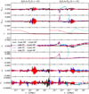 |
Fig. 17 Same Fig. 16 but now for the difference between the derivative of the logarithm of the linear (left) and nonlinear (right) matter power spectrum computed with one of CLASS DP or CAMB (with either P1, P2, or P3 precision) with the same derivative computed with CLASS HP. |
7 Conclusions
For the purpose of Euclid forecasts we have thoroughly validated the MP/Fisher pipeline against a bunch of CosmicFish Fisher forecast pipelines and a few other previous results from EP:VII. Despite of the very different method through which MontePython and CosmicFish compute Fisher matrices, we found a spectacular level of agreement between them. Typically, with pessimistic Euclid settings, all errors agree at least at the 2% level between the MP/Fisher and CosmicFish pipelines for both the photometric and spectroscopic cases. Even when involving additional forecast pipelines from EP:VII, all error bars agree much better than the “10% with respect to the median” threshold fixed by the latter group. We also showed that forecasts performed with CLASS or CAMB agree very well with each other, especially when both codes are called through their Python wrappers (leading to sub-0.5% differences between all errors computed with CF/int/CAMB versus CF/int/CLASS). Additionally, we proved that the Gaussian approximation on which all Fisher forecasts are relying is valid in the context of Euclid and of the ACDM+{w0, wa} model, since the Fisher ellipses overlap with the contours derived from an MCMC run using the same MontePython mock Euclid likelihoods.
This validation step is interesting by itself, because it allows us to cross-check the impact and the self-consistency of several details in the recipes used for modelling the Euclid photometric and spectroscopic probes and by the same occasion to validate some new ways of using the CosmicFish code with four different interfaces with the CAMB and CLASS Einstein-Boltzmann solvers. In the present paper we tried to document thoroughly all the physical assumptions and numerical methods used by these pipelines, reporting things exactly as they are implemented in the codes. We also reported our predictions for the sensitivity of Euclid to the parameters of the ΛCDM+{w0, wa} model when the photometric and spectroscopic probes are used either independently or in combination with each other.
However, in the context of preliminary work for Euclid the most important consequence of this work of validation is to pave the way to further robust forecasts. As a matter of fact any cos-mological model implemented in the CLASS code can now be immediately used in a forecast: for this, one just needs to add to the input file of MontePython one line per free parameter. If this parameter is known by CLASS, there is nothing else to be done. Thanks to the new CF/int/CAMB pipeline presented here, this is actually also true for any parameter or model implemented in CAMB. However, the version of the mock likelihoods used in this paper relies on a few model-dependent assumptions (such as the standard Poisson equation or the fact that galaxies trace the total matter power spectrum). These assumptions require some generalisation in the case of massive neutrinos or modified gravity models. A generalisation of the MontePython Euclid mock likelihoods to the case of massive neutrinos will be released soon (together with a forthcoming publication). Since MontePython calls the very same functions (describing the two Euclid mock likelihoods) when computing the Fisher matrix or when running an MCMC forecast, and since MP/Fisher forecasts have been validated against EP:VII forecasts, we automatically know that MP/MCMC forecasts can be trusted on equal footing with EP:VII forecasts, with the additional advantage of taking consistently into account a possible non-Gaussianity of the posteriors.
The MontePython Euclid mock likelihoods should not be confused with the official Euclid likelihood that is currently being developed within the collaboration. The latter is more ambitious and includes effects that are neglected here (such as super-sample covariance, different intrinsic alignment models, redshift-space distortions and magnification in the photometric galaxy clustering, or nonlinear galaxy biasing, just to name a few). Nonetheless, the MontePython Euclid likelihoods provide a robust tool against which the official likelihood can be compared and tested.
Another more general benefit from our analysis is that we have established and documented a list of accuracy settings for the EBSs CAMB and CLASS that prove to be sufficient for the purpose of Euclid forecasts, and thus, in principle, for the analysis of real Euclid data.
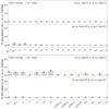 |
Fig. 18 For the photometric survey (top panels) and spectroscopic survey (bottom panels) both with optimistic settings, comparison of the Fisher marginalised and unmarginalised errors on each cosmological and nuisance parameters for CAMB P2 versus CAMB P3 precision (first and third panels), or CLASS DP versus HP precision (second and fourth panels). Plotting conventions are the same as in Fig. 2. |
Acknowledgements
N.S. acknowledges support from the Maria de Maetzu fellowship grant: CEX2019-000918-M, financiado por MCIN/AEI/10.13039/501100011033. N.F. is supported by the Italian Ministry of University and Research (MUR) through the Rita Levi Montalcini project “Tests of gravity on cosmic scales” with reference PGR19ILFGP. N.F. and F.P. also acknowledge the FCT project with ref. number PTDC/FIS-AST/0054/2021. S.V. acknowledges support funded by the Deutsche Forschungsgemeinschaft (DFG, German Research Foundation) under Germany’s Excellence Strategy – EXC-2121 “Quantum Universe” – 390833306. E.B. has received funding from the European Union’s Horizon 2020 research and innovation program under the Marie Skłodowska-Curie grant agreement No 754496. F.P. acknowledges partial support from the INFN grant InDark and the Departments of Excellence grant L.232/2016 of the Italian Ministry of University and Research (MUR). St.C. acknowledges support from the ‘Departments of Excellence 2018-2022’ Grant (L. 232/2016) awarded by the Italian Ministry of University and Research (MUR). Z.S. acknowledges funding from DFG project 456622116. The Euclid Consortium acknowledges the European Space Agency and a number of agencies and institutes that have supported the development of Euclid, in particular the Academy of Finland, the Agenzia Spaziale Italiana, the Belgian Science Policy, the Canadian Euclid Consortium, the French Centre National d’Études Spatiales, the Deutsches Zentrum für Luft- und Raumfahrt, the Danish Space Research Institute, the Fundação para a Ciência e a Tecnologia, the Ministerio de Ciencia e Innovación, the National Aeronautics and Space Administration, the National Astronomical Observatory of Japan, the Netherlandse Onderzoekschool Voor Astronomie, the Norwegian Space Agency, the Romanian Space Agency, the State Secretariat for Education, Research and Innovation (SERI) at the Swiss Space Office (SSO), and the United Kingdom Space Agency. A complete and detailed list is available on the Euclid web site (http://www.euclid-ec.org).
Appendix A Input and precision settings in Einstein–Boltzmann solvers
We list below the input parameter passed to either CAMB or CLASS in our Euclid forecasts. Section 6 discusses the relevance of precision parameter settings for such forecasts.
Appendix A.1 Fiducial cosmology parameters
We use the same fiducial value of cosmological parameters as in EP:VII: CAMB
use_physical = T # to pass big Omegas
sigma8 = 0.815584
hubble = 67
omega_baryon = 0.05
omega_m =0.32
scalar_spectral_index(1) =0.96
w = −1.0
wa = 0.0
dark_energy_model = PPF # use PPF scheme in DE
   perturbations, as in CLASS
helium_fraction = 0.2454006
temp_cmb = 2.7255 # relevant in neutrino mass conversion
reionization = F # Reio is irrelevant here. Switching it off gives a small
      #speedup. Not possible when CMB included.
We get the same fiducial cosmology in CLASS with the following settings: CLASS
sigma8 = 0.815584
h = 0.67
Omega_b = 0.05
Omega_m = 0.32
n_s = 0.96
w0_fld=−1.
wa_fld=0.
Omega_Lambda=0 # setting the true cosmological
   constant to zero, in order
      # to activate the DE fluid (fld) with a CPL equation of state
YHe = 0.2454006 # Helium fraction
T_cmb = 2.7255 # relevant in neutrino mass conversion reio_parametrization = reio_none
Appendix A.2 Neutrino settings
This issue is actually tricky because by default CAMB and CLASS model the details of the neutrino sector differently. The modelling used in CLASS aims at being closer to reality (that is, to the results of the most detailed studies of neutrino decoupling, such as Froustey et al. (2020); Bennett et al. (2021)). However, for the purpose of comparing our forecast pipelines – rather than fitting real data – the quest for realism is irrelevant: we just want the neutrino modelling to be reasonable and identical in the two codes. Then, it is easier to set up CLASS parameters in such way to mimic the CAMB neutrino model.
The CAMB neutrino model used here is the one corresponding to the option share_delta_neff = T, explained in its documentation website 20. The relevant neutrino parameters that we pass to CAMB are: CAMB
share_delta_neff = T
num_mass_eigenstates = 1
massless_neutrinos = 2.046
massive neutrinos = 1
mnu=0.06
In CAMBthese settings trigger several non-trivial operations, with the goal of having the same temperature shared by the three neutrino species. The true effective number of ultra-relativistic degrees of freedom (i.e. massless neutrinos) actually used in the CAMB equations is redefined internally from 2.046 to a new number:
![Mathematical equation: ${N_{{\rm{ur}}}} = 2 + {2 \over 3} \times (2.046 - {\rm{floor}}[2.046]) \simeq 2.030666{\rm{,}}$](/articles/aa/full_html/2024/02/aa46772-23/aa46772-23-eq103.png) (A.1)
(A.1)
while the massive neutrinos are modelled as a perfect Fermi-Dirac species with a temperature Tv and fractional density Ωv computed as
 (A.2)
(A.2)
To mimic exactly the same settings, we must pass these last numbers to CLASS:
CLASS
N_ncdm = 1
N_ur = 2.030666
T_ncdm = 0.7164864
Omega_ncdm = 0.001437166
Appendix A.3 Linear matter power spectrum settings
The following output settings allow CAMB and CLASS to output the matter power spectrum with a fine enough sampling to avoid interpolation errors within the likelihood codes.
CAMB
transfer_high_precision = T
transfer_kmax = 50
transfer_k_per_logint = 50
CLASS
P_k_max_h/Mpc = 50.
k_per_decade_for_pk = 50
k_per_decade_for_bao = 50
(The CosmicFish internal mode expects a kmax in units of 1/Mpc: in this case we pass P_k_max_l/Mpc = 50.)
Appendix A.4 Nonlinear power spectrum settings
The following parameters are only relevant for the photometric likelihood, which requires a nonlinear power spectrum in input. We stick to the choice of EP:VII to use the Halofit version of Takahashi et al. (2020), including neutrino corrections found by Bird et al. (2012) and implemented in both CAMB and CLASS:
CAMB
do_nonlinear = 1
halofit_version = 4
Besides, it is crucial to change the value of a tolerance parameter in the version of the Halofit algorithm implemented in CAMB. The file fortran/halofit.f90 contains a function THalofit_GetNonLinRatios() that computes a characteristic radius rmid with a bisection method. The bisection accuracy is set by the line
if (abs(diff).le.0.001) then
It is essential to substitute this tolerance by a new precision parameter or a hard-coded value equal to (or smaller than) 10−6. Otherwise, the error on rmid is way too large given the Euclid sensitivity, and leads to inaccurate derivatives in the Fisher matrix calculation. In our implementation, this new CAMB precision parameter is called halofit_tol_sigma. We discuss our settings for this parameter together with that of other important accuracy parameters in Appendix A.5.
The Halofit version implemented in CLASS coincides with the “Halofit version 4” of CAMB. We need to ask CLASS to use a large enough kmax for the sake of convergence of the Halofit algorithm even at high redshift: CLASS
non linear = halofit
nonlinear_min_k_max = 80.
Within CLASSthe tolerance parameter mentioned above is also called halofit_tol_sigma and set by default to 10−6, which proves to be sufficient for computing Euclid Fisher matrices with the CosmicFish method. However, as discussed in Appendix B.3, the calculation of Fisher matrices with the MontePython method requires even higher precision. We discuss our settings for this parameter together with that of other important accuracy parameters in Appendix A.5.
Appendix A.5 High-precision settings
High-precision settings slow down the two codes substantially, but they guarantee excellent mutual agreement between them, as well as a low level of numerical noise that allows us to compute numerical derivatives w.r.t. cosmological parameters using smaller stepsizes. These settings relate mainly to the multipole ℓmax at which the various Boltzmann hierarchies are truncated, to the sampling of perturbations in wavenumber space, to integration time steps and to the use of various approximation schemes.
For CAMBwe always use the following precision settings:
CAMB
do_late_rad_truncation = T
high_accuracy_default=T
transfer_interp_matterpower = T
accurate_reionization = F
There are three additional parameters playing a particularly important role, and for which we define three levels called P1, P2, P3:
CAMB(P1 / P2 / P3)
accuracy_boost =2/2/3
l_accuracy_boost =2/2/3
halofit_tol_sigma = 1.e-3 / 1.e–6 / 1.e–6
We compare P1, P2, and P3 in Sect. 6, but in the rest of this work we stick to P3.
For CLASSwe show in Sect. 6 that default precision (DP) is usually sufficient when computing the Euclid Fisher matrices with the CosmicFish method. However, the calculation of Fisher matrices with the MontePython method requires enhanced settings:
CLASS(HP)
l_max_g=20
l_max_pol_g=15
radiation_streaming_approximation = 2
radiation_streaming_trigger_tau_over_tau_k = 240.
radiation_streaming_trigger_tau_c_over_tau = 100.
tol_ncdm_synchronous = 1.e–5
l_max_ncdm=22
ncdm_fluid_trigger_tau_over_tau_k = 41.

background_Nloga = 6000
thermo_Nz_log = 20000
thermo_Nz_lin = 40000
tol_perturbations_integration = 1.e–6
halofit_tol_sigma = 1.e–8
The first eight parameters increase the precision of the system of perturbation equations (by truncating Boltzmann hierarchies at higher multipoles, better sampling neutrino momenta and using approximations in a smaller region). The next four parameters reduce the integration stepsize in the ordinary differential equations describing respectively the background, thermodynamical and perturbation evolution. They also reduce interpolation errors when the perturbation equations require the evaluation of background and thermodynamical quantities at a given value of the scale factor a. The last parameter reduces random errors in Halofit caused by a bisection algorithm.
Fiducial values and MCMC marginalised errors for all free parameters in the photometric probe.
In DP mode none of these parameters are passed to the code. We illustrate the impact of DP versus HP in Sec. 6, and we stick to HP everywhere else when computing Fisher matrices. Instead, for MCMC runs we always stick to DP settings.
Appendix B Fiducial parameter and choice of step sizes
Appendix B.1 Fiducial parameters
In Table B.1 (resp. Table B.2), we summarise our choice of fiducial values and step sizes for the cosmological and nuisance parameters of the photometric (resp. spectroscopic) probe. The fiducial values are the same as in EP:VII. In the last two columns of each table we show the marginalised errors (inferred from MCMC runs), which play a role in the discussion of Fig. B.3.
Appendix B.2 Stepsizes in CosmicFish
In EP:VIIthe different codes always computed the first-order derivatives ∂αCℓ or ∂αP(k,µ, z) with the SteM method or the n-point stencil method, which rely on the evaluation of the Cℓ’s or P(k, z) at a few different values of the parameter pα – see Appendix B of Camera et al. (2017) forfurtherdetails. However, in this work, we checked explicitly that the CosmicFish results stay the same when switching to a simpler two-sided derivative scheme, with steps roughly of the order of 1% of the fiducial parameter values (or 0.01 in the case of w0and wa).
We attribute this feature mainly to our use of higher precision settings in CAMB, and in particular to the reduction of the tolerance parameter of CAMB’s Halofit version from 10−3 to 10−8, see Appendix A.4. This leads to a significant reduction of the numerical noise in the CAMB output, mainly for nonlinear spectra used by the photometric probe. Thus, it removes the need to average the noise over several output spectra, as done implicitly within the SteM scheme. The main CosmicFish results of this work have been obtained with step sizes set to exactly 1% of the fiducial values of Table B.1 and B.2 (or to 0.01 for w0 and wa). We checked that changing the step sizes by a factor two does not impact the results. CosmicFish does not use a finite difference method to evaluate derivatives with respect to the shot noise parameters because these are trivial (for α = p(zi·), one gets ∂α Pobs = 1).
Appendix B.3 Stepsizes in MontePython/Fisher
Since the MP/Fisher and CosmicFish pipelines need to compute some intrinsically different numerical derivatives (second derivatives of ℒ versus first derivatives of Cℓ’s or P(k)’s), the step sizes also need to be optimised independently in the two cases.
When the step sizes are too small, there is a risk that the difference Δℒ between likelihood values computed at (pα ± Δpα, pβ ± Δpβ) is dominated by numerical errors rather than physical effects. When the step sizes are too big, we may exit from the region in which the likelihood is Gaussian, that is, χ2(p1, …,pN) is quadratic. The χ2 would then pick up higher order contributions, starting from cubic terms. As a result, the matrix ∂α∂β(− lnℒ) would strongly depend on step sizes and would no longer represent the Fisher matrix.
Fiducial values and MCMC marginalised errors for all free parameters in the spectroscopic probe.
If the precision of the EBS and of the likelihood code are sufficient, there should exist a range of intermediate step sizes such numerical noise is under control while Fij is nearly constant as a function of step sizes. This can be checked explicitly. For diagonal coefficients of the Fisher matrix, one can plot  as a function of the step Δpα. One should be able to see three regions: for too small Δpα, Fαα should feature random fluctuations; For intermediate Δpα, it should remain flat; For too large Δpα, it should either raise or decrease, depending on the sign of higher order corrections. For non-diagonal coefficients one may plot Fαβ as a two-dimensional function of (Δpα, Δpβ), and draw similar conclusions.
After performing such tests, one can choose some arbitrary step sizes provided that they lay within the intermediate region. These tests also allow us to check the accuracy of the Einstein–Boltzmann and likelihood codes. If both codes are accurate enough for the purpose of computing the Fisher matrix, there exist a wide range of intermediate step sizes for each parameter. If one of the codes is not sufficiently accurate, there is no intermediate region, that is, derivative curves show no transition between the unstable region and the non-Gaussian region.
Since doing all these tests can be very time-consuming, we do not want to perform them extensively before each new calculation of a Fisher matrix. In this work, we adopt a pragmatic approach:
We first compute the marginalised errors on each parameter pα, σ™^, using either CosmicFish, or MP/MCMC runs, or preliminary runs of MP/Fisher - this makes no difference. We set these σ™8^ as reference values with respect to which we can calibrate our step sizes. Our values of σ™^ are listed in the last two columns of Tables B.1 and B.2.
We compute a few diagonal and non-diagonal Fisher matrix elements Fαß with the step sizes (Δpα = x σ^\Δpß = x σ™^) for various values of x (typically in the range 0.01 < x < 1) and we plot the curves FαjS(x).
We check that there exist an intermediate range of values of x such that the curves are stable and flat. If not, we push the accuracy settings of the codes and we start the test again. If yes, we choose an arbitrary value of x sitting comfortably within the intermediate region.
Once this test has been done once for each probe, we can make general recommendations to use a given accuracy in the codes and to set correctly the order of magnitude of the steps relatively to the marginalised errors.
Then, there is no need to repeat this test again and again. The user can trust the fact that with such recommendations, the Fisher matrix is accurate and stable against small variations of the step sizes. At most, as a cross-check, the user can try once to increase or decrease all step sizes (for instance, by ~30%), recompute the Fisher matrix, and verify that it remains stable.
We have performed such tests for each probe and for a few matrix elements Fαß. We focused particularly on the non-diagonal element FW0 Wa, which is among the most difficult ones to compute accurately given the strong correlation between W0 and Wa.
For each probe, we have computed the function FW0 Wa(x) for 40 values of x ranging from 0.025 to 1 with a spacing Δx = 0.025, while using CLASS with either the default-precision (DP) or high-precision (HP) settings defined in Appendix A.5. Once the value of x has been set, we multiply it with the marginalised errors of Tables B.1 and B.2 to get our actual step sizes (these errors are derived from our MCMC runs, but we could have indifferently taken some marginalised errors from CosmicFish). For sufficiently large values of x the points lay on a parabola (FW0 Wa (x) o x2) that corresponds to the leading-order deviation from a Gaussian likelihood (since an exact Gaussian likelihood would give FW0 Wa(x) = constant). This happens typically for x > 0.1 with HP or above a larger threshold with DP. We then infer the asymptotic value FW0Wa (0) from a parabolic fit to the set of points computed with high-precision settings in the range 0.1 < x < 1. Finally, in Fig. B.1, we show the quantity
 (B.1)
(B.1)
as a function of the step-size-to-error ratio x = Δpαiσ^a%', for each accuracy setting. The quantity y can be considered as the percentage error on the estimate of the second derivative FW0 Wa(x) that comes from random numerical noise or the non-Gaussianity of the likelihood, that is, from the kind of errors that can be controlled by an adequate step size. (Of course, y does not include contributions from some possible systematic errors in the EBS or in the likelihood code, but we can estimate those errors independently from the CAMB-versus-CLASS and CosmicFish-versus-MontePython comparison of Sect. 4.) We computed y(x) in the range 0.025 ≤ x ≤ 1, but in Fig. B.1 we only show the range 0.025 ≤ x ≤ 0.4 which is the most interesting (for larger x, we obtain a nearly perfect parabola).
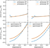 |
Fig. B.1 Percentage error on the estimate of the second derivative |

For the photometric survey Fig. B.1 shows that, with DP, the points feature random fluctuations below x < 0.2. Indeed, when computing the Fisher matrix, we get unstable results with DP and such small step sizes (for instance, the inverse Fisher matrix is not always positive definite and the marginalised errors fluctuate a lot with the step size). The solution consists in switching to HP: then, the points follow smoothly the parabola down to x ~ 0.1 and even lower. Additionally, we see that non-Gaussian corrections are small: even at x = 0.4 they affect  by only 0.1% (resp. 0.04%) in the pessimistic (resp. optimistic) case. As expected, the optimistic case features a more Gaussian likelihood (thanks to its enhanced constraining power). Our overall recommendation for the photometric survey is to use HP settings with an x roughly in the range [0.1,0.5], although it would also be possible to get good result while sticking to DP with x roughly in the range [0.3, 0.5]. We did various tests to check explicitly that with such recommendations, we always get stable predictions for all unmarginalised and marginalised errors. However, in the result sections, we always used HP and x = 0.1. The absolute step sizes Δpα for the pessimistic and optimistic cases are thus given by the last two columns of Table B.2 divided by 10.
For the spectroscopic survey Fig. B.1 shows that with either DP or HP the points are smoothly distributed and follow a parabola for any x ≥ 0.05. The non-Gaussianity is much stronger in this case: with x = 0.4 the error on  reaches 1% (resp. 0.5%) in the pessimistic (resp. optimistic) case. Thus one should restrict to x < 0.1 in order to keep the non-Gaussian contamination below approximately 0.1%. For x in the range [0.05,0.1], the DP and HP points are always following a smooth parabola, and indeed we checked that the Fisher matrix and errors are Article number, page 28 of 33 always stable in this range. However, the results obtained with HP are more correct because the physical effects of the parameters are captured with higher accuracy. In Fig. B.1 this appears in the form of an overall shift of FW0 Wa by approximately -0.1% when sticking to DP. We observed similar shifts in other elements of the Fisher matrix. Instead, when further increasing precision beyond our HP settings, we checked that the results remain stable. Between DP and HP, the (un)marginalised Fisher errors only move by one or two percent, but for better accuracy we recommend using HP with x in the range [0.05,0.1]. In the result sections we always used HP and x = 0.05. The absolute step sizes Δpα for the pessimistic and optimistic cases are then equal to the last two columns of Table B.2 divided by 20.
Appendix C Contour plots for nuisance parameters
Appendix C.1 Photometric survey with pessimistic settings
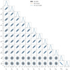 |
Fig. C.1 For the photometric survey with pessimistic settings, comparison of 1D posterior and 2D contours (for 68% and 95% confidence level) from different methods: MP/MCMC (grey lines/contours), MP/Fisher (orange lines), CF/int/CLASS (blue lines). We only show here the nuisance parameters. The triangle plot for cosmological parameters was shown in the main text. Plotted using GetDist. |
Appendix C.2 Spectroscopic survey with optimistic and pessimistic settings
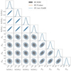 |
Fig. C.3 Same as Fig. C.1 for the nuisance parameters of the spectroscopic survey with pessimistic settings. For illustration purposes, we have labelled the parameters ln[biσ8(z1)] as ln(bs8i). |
Appendix D Contour plots for combined probes with pessimistic settings
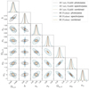 |
Fig. D.1 For the individual and combined photometric and spectroscopic surveys with pessimistic settings, 1D posterior and 2D contours on cosmological parameters from CF/int/CLASS (dotted lines) and MP/Fisher (solid lines). Plotted using GetDist. |
References
- Audren, B., Lesgourgues, J., Benabed, K., & Prunet, S. 2013a, J. Cosmol. Astropart. Phys., 02, 001 [NASA ADS] [CrossRef] [Google Scholar]
- Audren, B., Lesgourgues, J., Bird, S., Haehnelt, M. G., & Viel, M. 2013b, J. Cosmol. Astropart. Phys., 01, 026 [CrossRef] [Google Scholar]
- Bennett, J. J., Buldgen, G., De Salas, P. F., et al. 2021, J. Cosmol. Astropart. Phys., 04, 073 [CrossRef] [Google Scholar]
- Bird, S., Viel, M., & Haehnelt, M. G. 2012, MNRAS, 420, 2551 [Google Scholar]
- Blas, D., Lesgourgues, J., & Tram, T. 2011, J. Cosmol. Astropart. Phys., 07, 034 [CrossRef] [Google Scholar]
- Boyle, A., & Komatsu, E. 2018, J. Cosmol. Astropart. Phys., 03, 035 [CrossRef] [Google Scholar]
- Brinckmann, T., & Lesgourgues, J. 2019, Phys. Dark Univ., 24, 100260 [Google Scholar]
- Brinckmann, T., Hooper, D. C., Archidiacono, M., Lesgourgues, J., & Sprenger, T. 2019, J. Cosmol. Astropart. Phys., 01, 059 [CrossRef] [Google Scholar]
- Camera, S., Harrison, I., Bonaldi, A., & Brown, M. L. 2017, MNRAS, 464, 4747 [NASA ADS] [CrossRef] [Google Scholar]
- Carron, J. 2013, A&A, 551, A88 [NASA ADS] [CrossRef] [EDP Sciences] [Google Scholar]
- Chevallier, M., & Polarski, D. 2001, Int. J. Mod. Phys. D, 10, 213 [Google Scholar]
- Euclid Collaboration (Blanchard, A. et al.) 2020, A&A, 642, A191 [NASA ADS] [CrossRef] [EDP Sciences] [Google Scholar]
- Euclid Collaboration (Pocino, A., et al.) 2021, A&A, 655, A44 [NASA ADS] [CrossRef] [EDP Sciences] [Google Scholar]
- Froustey, J., Pitrou, C., & Volpe, M. C. 2020, J. Cosmol. Astropart. Phys., 12, 015 [CrossRef] [Google Scholar]
- Hamann, J., Balbi, A., Lesgourgues, J., & Quercellini, C. 2009, J. Cosmol. Astropart. Phys., 04, 011 [CrossRef] [Google Scholar]
- Kaiser, N. 1987, MNRAS, 227, 1 [Google Scholar]
- Lesgourgues, J. 2011a, arXiv e-prints [arXiv: 1104.2932] [Google Scholar]
- Lesgourgues, J. 2011b, arXiv e-prints [arXiv: 1104.2934] [Google Scholar]
- Lesgourgues, J., & Tram, T. 2014, J. Cosmol. Astropart. Phys., 09, 032 [CrossRef] [Google Scholar]
- Lewis, A. 2019, arXiv e-prints [arXiv: 1910.13970] [Google Scholar]
- Lewis, A., Challinor, A., & Lasenby, A. 2000, ApJ, 538, 473 [Google Scholar]
- Linder, E. V. 2003, Phys. Rev. Lett., 90, 091301 [Google Scholar]
- Naidoo, K., Johnston, H., Joachimi, B., et al. 2023, A&A, 670, A149 [NASA ADS] [CrossRef] [EDP Sciences] [Google Scholar]
- Percival, W. J., Burkey, D., Heavens, A. et al. 2004, MNRAS, 353, 1201 [NASA ADS] [CrossRef] [Google Scholar]
- Raveri, M., Martinelli, M., Zhao, G., & Wang, Y. 2016, arXiv e-prints [arXiv: 1606.06268] [Google Scholar]
- Sprenger, T., Archidiacono, M., Brinckmann, T., Clesse, S., & Lesgourgues, J. 2019, J. Cosmol. Astropart. Phys., 02, 047 [CrossRef] [Google Scholar]
- Takahashi, R., Nishimichi, T., Namikawa, T., et al. 2020, ApJ, 895, 113 [NASA ADS] [CrossRef] [Google Scholar]
- van den Busch, J. L., Hildebrandt, H., Wright, A. H., et al. 2020, A&A, 642, A200 [NASA ADS] [CrossRef] [EDP Sciences] [Google Scholar]
- Virtanen, P., Gommers, R., Oliphant, T. E., et al. 2020, Nat. Methods, 17, 261 [Google Scholar]
- Yahia-Cherif, S., Blanchard, A., Camera, S., et al. 2021, A&A, 649, A52 [NASA ADS] [CrossRef] [EDP Sciences] [Google Scholar]
This was not the case for all the algorithms used in EP:VII: for the photometric probe, two of the pipelines could call directly the EBS instead of storing its results in files.
In the context of forecasts the best fit is simply the assumed fiducial model.
In typical forecasts there is no actual observed data. Instead, the fiducial model (referred here as “fid”) is used to emulate a possible observation.
There exists another option: one may use a likelihood that is Gaussian in the C(ℓ)’s instead of the aℓm’s. The EP:VII paper uses both methods to compute the Fisher matrix forecasts, showing that they are equivalent for all our practical purposes. See Eq. (142) and Eq. (143) in EP:VII for details.
Note that EP:VII uses an equivalent expression in which the spectrum that appears in Eq. (10) does not include shot noise, while here we do assume that  and
and  include shot noise. In the conventions of EP:VII, to compensate for this,
  needs to be replaced by
 (11)
(11)
where  is the galaxy number density in each redshift bin and the product
  is dimensionless.
The release will take place upon acceptance of this paper as an update of the main MontePython branch in the public repository.
Notice that a more realistic photometric distribution based on the Euclid Consortium Flagship was recently published in Euclid Collaboration (2021). However, for the sake of validation, we stick to the analytic formula used in EP:VII.
This technical detail is important for calculating derivatives with respect to the bi’s. Thus it is necessary to stick to the same convention in order to recover a similar Fisher matrix. In the codes the second option (used here) is called binned, while the first option is called binned_constant.
We are assuming equally populated bins as in EP:VII.
We recall that when the growth factor D and growth rate f are expressed as a function of the scale factor a, they are related to each other through f (a) = d ln D(a)/d ln a.
In Fig. 2 each panel presents a comparison between two cases only. Thus the median is just the average of the two errors and the plotted discrepancy stands for one half of the relative difference between the two errors. In other figures such as in Fig. 3 the median is instead computed across four different cases.
The extremely small (0.02%) differences can be attributed to very small details in the sampling of functions, rounding errors when writing in files, etc. They are totally irrelevant at the Euclid sensitivity level.
The small deviation of the CF/ext/CAMB pipeline with respect to the other ones may have to do with a small unexplained feature in the derivative of the nonlinear power spectrum with respect to wa observed in Fig. B.1 of Appendix B.2. We leave this issue for future investigation.
In this section we only compared the linear and nonlinear power spectra from CAMB and CLASS. Internally, we also compared the functions D(z), f(z), and σ8(z). For the latter, we did not find any noticeable difference that would be worth reporting.
All Tables
Redshift-dependent survey specifications evaluated at the central redshift zi of each redshift bin.
For the photometric survey with pessimistic settings, and for each pair of Fisher matrices obtained with different methods, largest percentage difference between the predicted marginalised error on each parameter (across all cosmological and nuisance parameters).
For the photometric survey with pessimistic settings, marginalised 1σ errors on cosmological parameters found by: the average of EP:VII results, CF/int/CLASS (the other versions of CosmicFish give nearly the same results), MontePython in Fisher mode, MontePython in MCMC mode.
For the combined photometric and spectroscopic surveys with various combinations of pessimistic and optimistic settings, marginalised 1σ errors on cosmological parameters found by CF/int/CLASS (the other versions of CosmicFish give nearly the same results).
Dark energy Figure of Merit for the spectroscopic survey with optimistic and pessimistic settings, found by: the determinant of the CosmicFish Fisher matrix and the area of the MontePython MCMC contours.
Fiducial values and MCMC marginalised errors for all free parameters in the photometric probe.
Fiducial values and MCMC marginalised errors for all free parameters in the spectroscopic probe.
All Figures
|
Fig. 1 Underlying theoretical distribution of the number density of galaxies n(z) (black dashed line), normalised to one, together with the ni(z) (solid colored lines) at each of the 10 tomographic redshift bins (dotted vertical colored lines), normalised to 1/10. The ni(z) are wide and overlap each other due to the photometric redshift errors. |
| In the text | |
|
Fig. 2 For the photometric survey with pessimistic settings, and for selected pair of Fisher matrices obtained with different methods, comparison of each Fisher marginalised (blue dot/light grey) and unmarginalised (orange dot/dark grey) error on each cosmological and nuisance parameters, for: (First) CF/ext/CAMB versus CF/int/CAMB; (Second) CF/ext/CLASS versus CF/int/CLASS; (Third) CF/int/CLASS versus CF/int/CAMB; (Fourth) CF/int/CLASS versus MP/Fisher. Each forecasted error σi for each case and parameter is compared to the median of the two cases (see footnote 13). The discrepancy is expressed in percent. |
| In the text | |
|
Fig. 3 For the photometric survey with pessimistic settings, comparison of each Fisher marginalised (light grey) and unmarginalised (dark grey) errors on the cosmological and nuisance parameters, for: CF/int/CLASS (blue circles) versus CF/int/CAMB (orange squares) versus MP/Fisher (green stars) versus the public EP:VII results (red crosses, referred in the legend as IST:F). Each forecasted error σi for each case and parameter is compared to the median of the four cases, and the discrepancy is expressed in percent. |
| In the text | |
|
Fig. 4 For the photometric survey with pessimistic settings, comparison of 1D posteriors and 2D contours (for 68 and 95% confidence level) from different methods: MP/MCMC (grey lines/contours), MP/Fisher (orange lines), CF/int/CLASS (blue lines). We only show here the cos-mological parameters, but our contours involving nuisance parameters are shown in Appendix C. Plotted using GetDist. |
| In the text | |
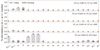 |
Fig. 5 Same as Fig. 2 with optimistic settings. |
| In the text | |
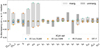 |
Fig. 6 Same as Fig. 3 with optimistic settings. |
| In the text | |
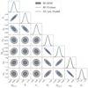 |
Fig. 7 Same as Fig. 4 with optimistic settings. |
| In the text | |
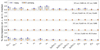 |
Fig. 8 Same as Fig. 2 for the spectroscopic survey with pessimistic settings. |
| In the text | |
|
Fig. 9 For the spectroscopic survey with pessimistic settings, comparison of each Fisher marginalised (light grey) and unmarginalised (dark grey) errors on the cosmological and nuisance parameters, for the cases of: CF/int/CLASS (blue circles) versus CF/int/CAMB (orange squares) versus MP/Fisher (green stars) versus EP:VII results from SOAPFish (SF, red crosses). Plotting conventions are the same as in Fig. 3. |
| In the text | |
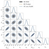 |
Fig. 10 Same as Fig. 4 for the spectroscopic survey with pessimistic settings. |
| In the text | |
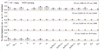 |
Fig. 11 Same as Fig. 2 for the spectroscopic survey with optimistic settings. |
| In the text | |
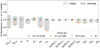 |
Fig. 12 Same as Fig. 9 with optimistic settings. |
| In the text | |
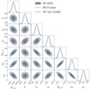 |
Fig. 13 Same as Fig. 4 for the spectroscopic survey with optimistic settings. |
| In the text | |
|
Fig. 14 For the individual and combined photometric and spectroscopic surveys with optimistic settings, 1D posterior and 2D contours (for 68% and 95% confidence level) on cosmological parameters from CF/int/CLASS (dotted lines) and MP/Fisher (solid lines). Plotted using GetDist. |
| In the text | |
|
Fig. 15 For the linear (left) and nonlinear (right) matter power spectrum of the fiducial model at redshift z = 0 (top) and z = 2 (bottom), percentage difference between the predictions of CLASS and CAMB. Here, the reference is the CLASS high-precision (HP) result. We compare it with CLASS Default Precision (DP) and CAMB with the precision settings defined as P1, P2, P3 in the text. In the linear case (left), the CAMB P1 curve is always overdrawn by the P2 one, since the difference between P1 and P2 is only relevant at the level of the nonlinear spectrum. |
| In the text | |
|
Fig. 16 Derivative of the logarithm of the linear (left) and nonlinear (right) matter power spectrum with respect to each cosmological parameter in our basis, computed with CLASS (with either DP or HP) and CAMB (with either P1, P2, or P3 precision). The derivatives are computed at z = 0. In the linear case (left), the CAMB P1 curve is always overdrawn by the P2 one, since the difference between P1 and P2 is only relevant at the level of the nonlinear spectrum. Moreover, P2 is always nearly overdrawn by P3. |
| In the text | |
|
Fig. 17 Same Fig. 16 but now for the difference between the derivative of the logarithm of the linear (left) and nonlinear (right) matter power spectrum computed with one of CLASS DP or CAMB (with either P1, P2, or P3 precision) with the same derivative computed with CLASS HP. |
| In the text | |
|
Fig. 18 For the photometric survey (top panels) and spectroscopic survey (bottom panels) both with optimistic settings, comparison of the Fisher marginalised and unmarginalised errors on each cosmological and nuisance parameters for CAMB P2 versus CAMB P3 precision (first and third panels), or CLASS DP versus HP precision (second and fourth panels). Plotting conventions are the same as in Fig. 2. |
| In the text | |
|
Fig. B.1 Percentage error on the estimate of the second derivative |
| In the text | |
|
Fig. C.1 For the photometric survey with pessimistic settings, comparison of 1D posterior and 2D contours (for 68% and 95% confidence level) from different methods: MP/MCMC (grey lines/contours), MP/Fisher (orange lines), CF/int/CLASS (blue lines). We only show here the nuisance parameters. The triangle plot for cosmological parameters was shown in the main text. Plotted using GetDist. |
| In the text | |
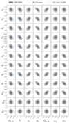 |
Fig. C.2 Same as Fig. C.1 for the correlation between cosmological and nuisance parameters. |
| In the text | |
|
Fig. C.3 Same as Fig. C.1 for the nuisance parameters of the spectroscopic survey with pessimistic settings. For illustration purposes, we have labelled the parameters ln[biσ8(z1)] as ln(bs8i). |
| In the text | |
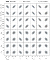 |
Fig. C.4 Same as Fig. C.3 for the correlation between cosmological and nuisance parameters. |
| In the text | |
|
Fig. D.1 For the individual and combined photometric and spectroscopic surveys with pessimistic settings, 1D posterior and 2D contours on cosmological parameters from CF/int/CLASS (dotted lines) and MP/Fisher (solid lines). Plotted using GetDist. |
| In the text | |
Current usage metrics show cumulative count of Article Views (full-text article views including HTML views, PDF and ePub downloads, according to the available data) and Abstracts Views on Vision4Press platform.
Data correspond to usage on the plateform after 2015. The current usage metrics is available 48-96 hours after online publication and is updated daily on week days.
Initial download of the metrics may take a while.