| Issue |
A&A
Volume 709, May 2026
|
|
|---|---|---|
| Article Number | A10 | |
| Number of page(s) | 16 | |
| Section | Galactic structure, stellar clusters and populations | |
| DOI | https://doi.org/10.1051/0004-6361/202557076 | |
| Published online | 28 April 2026 | |
STEP survey
III. STEPping stones between the clouds: the star formation history of the Magellanic Bridge★
1
INAF – Osservatorio Astronomico di Capodimonte,
Salita Moiariello 16,
80131
Napoli,
Italy
2
Università di Salerno, Dipartimento di Fisica “E.R. Caianiello”,
Via Giovanni Paolo II 132,
84084
Fisciano (SA),
Italy
3
Dipartimento di Fisica, Università di Pisa,
Largo Bruno Pontecorvo 3,
56127,
Pisa,
Italy
4
INAF – Osservatorio di Astrofisica e Scienza dello Spazio di Bologna,
via Piero Gobetti 93/3,
40129
Bologna,
Italy
5
INFN,
Largo B. Pontecorvo 3,
56127
Pisa,
Italy
6
Astronomisches Rechen-Institut, Zentrum für Astronomie der Universität Heidelberg,
Mönchhofstraße. 12-14,
69120
Heidelberg,
Germany
7
Leibniz-Institut für Astrophysik Potsdam,
An der Sternwarte 16,
14482
Potsdam,
Germany
8
INFN – Gruppo Collegato di Salerno-Sezione di Napoli, Dipartimento di Fisica “E.R. Caianiello”, Università di Salerno,
Via Giovanni Paolo II, 132,
84084
Fisciano (SA),
Italy
★★ Corresponding author.
Received:
2
September
2025
Accepted:
11
February
2026
Abstract
Context. The Magellanic Clouds (MCs) offer a unique laboratory for studying galaxy interaction and the evolution of dwarf galaxies. The star formation history (SFH), which traces when and how stars formed, provides powerful constraints for the dynamical modelling of the system’s past interactions and the processes of stripping and triggered star formation in tidally influenced environments.
Aims. We aim to reconstruct the SFH of the Magellanic Bridge, the gaseous and stellar stream connecting the Magellanic Clouds. We used data from the deep optical STEP survey, which covers 54 deg2 across the Small Magellanic Cloud (SMC) and the Bridge, reaching stars below the oldest main-sequence turnoff at the distance of the MCs.
Methods. We applied the synthetic colour-magnitude diagram technique to 14 deg2 of STEP data. We constructed two libraries of synthetic stellar populations based on the PARSEC-COLIBRI and BaSTI stellar evolutionary models, with metallicities in the range −2.0 ≤ [Fe/H] ≤ 0 across the whole Hubble time.
Results. We find a clear peak of recent star formation ∼100 Myr ago in the Magellanic Bridge, which becomes increasingly pronounced towards the SMC. The low metallicity of this population suggests that it formed from gas stripped from the SMC during its most recent close encounter with the LMC. In the eastern part of the Bridge (LMC side), star formation peaks at earlier times, around 10 Gyr and 2 Gyr ago. We estimate a total stellar mass in the Bridge of (5.1 ± 0.2) × 105M⊙ and a present-day stellar metallicity of [Fe/H]~-0.6 dex, close to SMC value.
Key words: Hertzsprung-Russell and C-M diagrams / galaxies: dwarf / galaxies: interactions / galaxies: irregular / Magellanic Clouds / galaxies: star formation
Based on data products from observations collected at the European Organization for Astronomical Research in the Southern Hemisphere, under ESO programs 099.D-0673(A); 098.D-0579(A); 097.D0209(A); 096.D-0535(A); 095.D-0132(A); 094.D-0492(A); 093.D0174(A); 092.D-0214(A); 091.D-0574(A); 090.D-0172(A); 089.D0258(A); and 088.D-4014(A).
© The Authors 2026
 Open Access article, published by EDP Sciences, under the terms of the Creative Commons Attribution License (https://creativecommons.org/licenses/by/4.0), which permits unrestricted use, distribution, and reproduction in any medium, provided the original work is properly cited.
This article is published in open access under the Subscribe to Open model. This email address is being protected from spambots. You need JavaScript enabled to view it. to support open access publication.
1 Introduction
The Small Magellanic Cloud (SMC) and the Large Magellanic Cloud (LMC) are the closest irregular galaxies orbiting the Milky Way (MW), and are considered the closest known pair of interacting dwarfs. According to the lambda cold dark matter (ΛCDM) model, smaller structures form first, then merge to create larger galaxies (White & Rees 1978; Moore et al. 1999; Stierwalt et al. 2017). Hence, dwarf galaxies, which reside in the smallest dark matter sub-halos, are considered optimal candidates for the role of ‘building blocks’ in galaxy formation. The Magellanic Clouds (MCs) provide an ideal laboratory for studying the evolution of interacting dwarf galaxies, as well as likely future contributors to the MW. Their proximity allows for deep observations with ground-based telescopes, enabling the reconstruction of their spatially resolved star formation histories (SFHs) with great detail. The LMC is a barred Magellanic spiral located at ∼50 kpc (Pietrzynski et al. 2019), while its smaller companion, the SMC, is a dwarf irregular (dIrr) galaxy at ∼62.5 kpc (Graczyk et al. 2020). Their mutual gravitational interactions have distorted the LMC’s disk (Haschke et al. 2012; Choi et al. 2018) and stretched the SMC along the line of sight, giving it an elongated shape (Jacyszyn-Dobrzeniecka et al. 2016; Ripepi et al. 2017). Despite ongoing efforts, the dynamical history of the Magellanic system remains only partially understood. Various substructures observed in the system, originating from the gravitational interactions between the SMC, the LMC and the MW offer key insights into its complex evolutionary past:
The Magellanic Stream is a complex network of gas, filaments, and clumps extending over 200 deg along the orbit of the MCs around the MW (Mathewson et al. 1974; Nidever et al. 2010). This structure consists of material stripped from both the LMC and SMC (Nidever et al. 2013a; Richter et al. 2013). While some hydrodynamic simulations attribute its origin to ram-pressure from the MW halo (Mastropietro et al. 2005; Wang et al. 2019), the prevailing view is that it formed from material stripped out from the MCs due to tidal interactions between them (D’Onghia & Fox 2016; Pardy et al. 2018; Lucchini 2024).
The leading arm stretches for ∼50 deg to the north-east of the LMC (Putman et al. 1998, 2003). It is thought to be the tidal counterpart of the Magellanic Stream, as its presence ahead of the MCs’ orbit may only be explained by tidal forces.
The Magellanic Bridge (Hindman et al. 1963) is a structure that connects the LMC to the eastern extension of the SMC, called the Wing, and consists of both metal-poor gas and a stellar component (Irwin et al. 1985). Most studies attribute its formation to the most recent interaction between the two Clouds, with material primarily stripped from the SMC (Gardiner & Noguchi 1996; Besla et al. 2012; Diaz & Bekki 2012). In addition to the H I gas distribution, the Bridge has been traced via its stellar content through its population of young blue stars (Irwin et al. 1990), star clusters (e.g. Bica et al. 2020) and variable stars (Jacyszyn-Dobrzeniecka et al. 2020a,b). Proper-motion studies reveal a net flow of stars from the SMC towards the LMC (Zivick et al. 2019; Schmidt et al. 2020; Gaia Collaboration 2021). The Bridge hosts both young stars and candidate older populations, though the latter are difficult to confirm due to low spatial density and contamination from the MW (Bagheri et al. 2013; Nidever et al. 2013b; Skowron et al. 2014). The most comprehensive study of the region’s SFH to date by Harris (2007) found no evidence for an old population of tidally stripped stars in the Bridge.
External substructures. The MCs are surrounded by an extended network of low surface-brightness stellar features resulting from their dynamical history. Both N-body simulations and observations indicate the presence of tidally distorted stellar populations (e.g. the formation of spirallike arms extending from the LMC disk (Belokurov & Erkal 2019; Cullinane et al. 2022; Gatto et al. 2022), likely induced by the combined tidal influence of the SMC and the MW. In the SMC, intermediate-age populations exhibit a pronounced elongation towards the Magellanic Bridge (El Youssoufi et al. 2019).
Even if the orbital history of the MCs is only partially understood, our knowledge has improved significantly. High-precision Hubble Space Telescope (HST) measurements of the MCs’ proper motions (Kallivayalil et al. 2006b,a) revealed that their velocities were too high for a system gravitationally bound to the MW. This overturned the traditional view of a longstanding bond (≳10 Gyr) between the MW and the MCs (Murai & Fujimoto 1980). This led to the ‘first passage’ scenario (Besla et al. 2007, 2012; Laporte et al. 2018; Lucchini et al. 2021), where the Magellanic system is on its first encounter with the MW1. This model is supported by the observed star formation (SF) and high gas content in the MCs, which would have likely been stripped away in repeated interactions, hindering SF. Indeed, other HI-rich dIrr satellites are typically found at greater distances from large spirals (Grebel et al. 2003; McConnachie 2012). The complex geometry of the MCs is more plausibly the result of interactions between the Clouds themselves (Besla et al. 2016; Choi et al. 2022), supported by the presence of a common H I envelope (van der Marel et al. 2009). Models involving repeated SMC-LMC encounters (Besla et al. 2011, 2012; Guglielmo et al. 2014; Pardy et al. 2018; Wang et al. 2019) successfully reproduce their asymmetric features and gas structures, as well as triggered bursts of SF observed in both galaxies. Their most recent close encounter is estimated to have occurred 150-250 Myr ago (Zivick et al. 2018, 2019; Schmidt et al. 2020; De Leo et al. 2020), an event that N-body models (Gardiner & Noguchi 1996; Guglielmo et al. 2014) predict led to the formation of the Bridge.
Even though the number and timing of past interactions remain uncertain, analysing their SFHs can reveal bursts of activity triggered by the gas compression from these encounters (Stierwalt et al. 2015). The SFH of the main bodies of the MCs has been extensively studied. Early investigations using HST provided unprecedentedly deep photometry of spatially small, localized regions within both galaxies (e.g. Holtzman et al. 1999; Dolphin et al. 2001; Sabbi et al. 2009; Cignoni et al. 2009, 2012, 2013; Weisz et al. 2013). However, these detailed snapshots were limited by small-number statistics due to HST’s small field of view. The radial age gradient behaves differently in the two galaxies. Meschin et al. (2014) found that in the outer LMC disk younger populations are increasingly concentrated towards smaller radii, indicating an outside-in quenching pattern. This is consistent with Cohen et al. (2024b), who show that the inner disk has an inside-out gradient that reverses beyond ~2 scale-lengths, with older stars at larger radii, likely due to radial migration. In contrast, the SMC exhibits a classical outside-in gradient, with older stars in the outskirts and ongoing SF in the central Wing (Cohen et al. 2024a). The advent of wide-field surveys has since enabled the reconstruction of the global SFH of the MCs. Key surveys that have driven this effort include:
Magellanic Clouds Photometric Survey (MCPS) (Zaritsky et al. 2002, 2004) is the first large-scale study of stellar populations in the MCs. Harris & Zaritsky (2004) found that about half of the SMC’s stars formed over ∼8.4 Gyr ago, followed by a prolonged period of quiescence. Subsequent bursts of SF occurred 2.5 Gyr, 400 Myr and 60 Myr ago, with counterparts at similar times in the LMC (Harris & Zaritsky 2009), indicating multiple past interactions.
VISTA survey of the Magellanic Clouds system (VMC) (Cioni et al. 2011, 2025) is a near-IR survey; Rubele et al. (2018) found that ∼50% of the stellar mass of the SMC formed over 6.3 Gyr ago, and confirmed that the older stellar population follows a smooth, elliptical distribution. The SMC’s bar and Wing exhibit a complex SFH, with multiple recent bursts. While the western part of the SMC experienced a relatively constant SF up to 1.5 Gyr ago, the eastern regions show two prominent peaks at 3.1 and 8 Gyr ago. The presence of stars younger than 200 Myr in the Wing supports the idea that a recent close encounter with the LMC triggered SF.
Survey of the Magellanic Stellar History (SMASH) (Nidever et al. 2017) provided further evidence of synchronized SF between the MCs. Massana et al. (2022) identified five peaks of SF in the SMC (3, 2, 1.1 and 0.45 Gyr ago, as well as an ongoing burst) aligned with bursts in the northern LMC (Ruiz-Lara et al. 2020), suggesting the galaxies synchronized their SF ∼3.5 Gyr ago, likely due to mutual gravitational interactions.
The goal of this paper is to derive the most extended SFH of the Magellanic Bridge employing deep optical data from the ‘Small Magellanic Cloud in Time: Evolution of a Prototype interacting late-type dwarf galaxy’ (STEP; Ripepi et al. 2014) survey, obtained using the VLT Survey Telescope (VST; Capaccioli & Schipani 2011). The paper is structured as follows: Section 2 outlines the STEP survey data, their processing, and the artificial star (AS) tests conducted. Section 3 discusses the synthetic colour-magnitude diagram (CMD) method, detailing the construction of our synthetic models, including the distances and extinctions applied to all analysed regions. In Section 4, we present the best-fit CMDs for selected regions and describe the results for the Magellanic Bridge as a whole. Finally, Section 5 summarises the key findings and outlines the main conclusions.
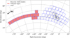 |
Fig. 1 Footprint of the STEP survey pointings (blue boxes), showing the location of the SMC body and the Bridge. The area covered by this work is highlighted in red. The LMC is in the left direction, outside the map. The black dots mark the position of star clusters and associations from the catalogue of Bica et al. (2020). |
2 The Magellanic Clouds in STEP
2.1 STEP data
STEP (Ripepi et al. 2014; Gatto et al. 2021) is a deep and extended photometric survey of the SMC and the Magellanic Bridge carried out with the 2.6m VLT Survey Telescope (VST), equipped with the wide-field imager Omegacam (Capaccioli & Schipani 2011; Kuijken 2011). The STEP survey covered the main body of the SMC and the Magellanic Bridge using the g, r, i and Hα filters (Fukugita et al. 1996; Gunn et al. 1998) at a limiting magnitude (g ~ 24 mag), which enables the detection of stars well below the turn-off of the oldest population (g ~ 23 mag in the SMC and ~22.5 mag in the LMC) with a signal-to-noise ratio of 10 (Ripepi et al. 2014), even in the most crowded regions, an ideal condition to reliably recover the SFH at all epochs. The entire survey covers a total area of 53 deg2. In this work, we focused on the Magellanic Bridge. To this end, we selected 14 tiles2, highlighted as shaded regions in the map in Fig. 1, where the approximate position of the SMC body and the Bridge are marked by star clusters and associations from Bica et al. (2020). The analysed region of the Bridge extends from right ascension (RA) α = 4h 28m 59s and declination δ = −73° 24′ 59j (tile 3_21, closer to the LMC, see Ripepi et al. 2014, for the identification of the tiles) to α = 2h 15m 00s and δ = −73° 24′ 59j (tile 3_11, on the SMC side).
2.2 Data reduction and photometry
Data reduction was performed using the VST-TUBE package (Grado et al. 2012), specifically developed to process OmegaCAM data from the VST telescope. The pipeline includes pre-reduction, astrometric and photometric calibration, as well as mosaic production. Further details on the reduction process are provided in Ripepi et al. (2014). Point-spread-function (PSF) photometry was carried out with the DAOPHOT IV/ALLSTAR package (Stetson 1987, 2011). To account for possible distortions at the edges of the tiles, the PSF function was allowed to vary across the field of view. The α and δ of each source were calculated using the package xy2sky, a utility that converts the image coordinates (X, Y) to equatorial coordinates using the world coordinate system (WCS) information in the image header. The absolute photometric calibration was obtained by using secondary standard stars in each tile as provided by the AAVSO Photometric All-Sky Survey (APASS) project3 (see Gatto et al. (2020) for further details). The photometric catalogue was cleaned of spurious objects, such as distant galaxies and artefacts caused by bad pixels, using the SHARPNESS parameter from the DAOPHOT package. This parameter measures how much broader a source appears compared to the PSF profile, enabling the removal of extended sources from the catalogue. The acceptance criteria for sources varied between tiles, with slightly different SHARP parameter ranges applied to each tile, usually around ±0.5 (see Table 3 for the SHARPNESS cut values used in each tile.). We provide the final catalogue, composed of 600 279 stars located within the Magellanic Bridge, for the scientific community. Table 1 offers an overview of the star-catalogue, whose full version is available at the CDS. To isolate the field stellar population for a cleaner analysis, we excluded stars associated with known clusters by cross-matching our data with the Bica et al. (2020) catalogue. A total of 13 clusters were removed, with stars excised if they fell within the major angular radii listed in the catalogue (ranging from 21″ to 1.2′, except for one cluster in tile 3_15, which extended to 2′ 27″). This process eliminated 225 stars from our data, averaging ∼20 stars per cluster, with a minimum of five and a maximum of 42 stars.
Photometric catalogue of the STEP survey in the Magellanic Bridge.
2.3 Artificial star tests
Two key factors for the reliability of the SFH estimated from PSF photometry are the photometric error and the incompleteness of the stellar photometry (Cignoni & Tosi 2010). The only accurate way to estimate these quantities across our magnitude range is by repeating the entire process of photometric measures on the science images on which ASs, of known position and magnitudes, are injected. To achieve a statistically reliable result, we generated a large number of AS (∼2-3 × 10⁶) with the appropriate Poisson noise and PSF, injecting them into each tile. These stars fully sample the range of magnitudes and colours covered by the data, spanning from g = 14 mag to 26 mag and a g - i colour range between −1.0 mag and 3.0 mag. The magnitude distribution of ASs is not uniform: 80% have g > 19 mag to better map completeness and photometric errors in the fainter regions of the CMD. Moreover, to avoid introducing additional crowding, the ASs are placed in the image on a grid with mutual distances much larger than the PSF, typically 10″ in our tests. The images containing real and ASs are then re-analysed with the DAOPHOT package. An AS is considered successfully recovered if its estimated position differs by less than 1 pixel (∼0.2″) from the input value, and if the recovered magnitude is not more than 0.75 mag brighter than the input one. In addition, we applied the same criteria for the SHARPNESS parameter to the ASs as we did for the real data. The completeness of our photometry was computed as the percentage of recovered ASs within each magnitude and colour interval, while photometric errors were derived as the difference in magnitude between the recovered and input AS in each filter. Our tests show that, across all regions of the Bridge, the STEP survey reaches 50% completeness at g ~ 23.5 mag and i ~ 23 mag, and at slightly fainter values in less crowded regions. To ensure a completeness level ≳50%, we applied a magnitude cut at g = 23.2 mag in all tiles in the recovery of the SFH. The estimated photometric error at the magnitude of the turn-off of the oldest population in the SMC (∼22.8) is ∼0.2 mag in the g filter. The fraction of recovered stars is best visualized in the CMD. By binning the CMD, we can construct 2D histograms (‘Hess diagrams’) that depict the frequency of stars in each colour-magnitude cell. Figure 2 shows the Hess diagrams with the completeness distributions of all tiles, where the 50% completeness level (typically at g ~ 23.2 mag for g - i = 0) is marked by a red line. To obtain a smooth distribution, we used a relatively large cell size of 0.1 mag in colour and 0.2 mag in magnitude. Figure 3 illustrates the photometric error as a function of the input magnitude in g and i, where the central red line marks the median of the distribution, which becomes negative for fainter stars due to the effects of blending.
3 The SFH recovery method
A complex mix of heterogeneous stellar populations can be analysed comparing the data against synthetic populations, employing the well-established ‘synthetic CMD’ approach (see e.g. Tosi et al. 1991; Tolstoy & Saha 1996; Dolphin 1997, 2002; Hernandez et al. 1999; Aparicio & Hidalgo 2009; Cignoni & Tosi 2010; Weisz et al. 2012). The SFH recovery was performed using SFERA (Star Formation Evolutionary Recovery Algorithm Cignoni et al. 2009, 2015), which utilizes Pikaia (Charbonneau 1995), a genetic algorithm that efficiently explores the parameter space independently of initial conditions. In our work, we built two catalogues of isochrones covering the age range from 10 Myr to 13.4 Gyr and [Fe/H] from −2.0 to 0.0 dex. For our study, we adopted the PARSEC-COLIBRI (Bressan et al. 2012; Marigo et al. 2017) and BaSTI (Hidalgo et al. 2018) stellar isochrones. In both sets of models we used solar-scaled abundances, convective overshooting, and a Reimers mass-loss parameter of η = 0.3. We grouped these isochrones into quasi-simple stellar populations (QSSPs or partial models), representing finite-duration episodes of constant SF. Each QSSP covers a specific time-span (see Table 2) and includes stars uniformly distributed within a small metallicity interval (0.1 dex). To populate the QSSPs, we employed a Monte Carlo approach, randomly selecting metallicity, age, and mass. The effective temperature Teff and luminosity L of each synthetic star were then assigned by interpolating along the isochrone of appropriate age.
To avoid under-populating the upper end of the mass spectrum, mass values were drawn from a uniform distribution between the hydrogen-burning limit (0.1 M⊙) and the maximum mass that is still alive at the corresponding model age. Each star was assigned a statistical weight, based on its formation probability derived from a Kroupa (2001) initial mass function (IMF). The presence of unresolved binaries alters the morphology of the CMD, and we needed to include this effect in our models: 30% of the synthetic stars were assumed to be unresolved binaries and the mass of the secondary star was randomly extracted from a Kroupa (2001) IMF. In the creation of binaries, we only simulated the photometric effect of seeing the fluxes of two stars as one single object when we populated the synthetic model. To ensure a proper representation of all stellar evolutionary phases, including rapid ones, each model was populated with a high number (106) of synthetic stars. In the end, we generated two libraries, each containing partial models of 19 different ages and 20 different metallicities (380 per library). Before comparing these models with our observations, we convolved them with the data characteristics, as described in the following sections.
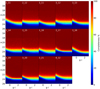 |
Fig. 2 Hess diagrams of the completeness for all analysed tiles. In each cell of the CMD the completeness is computed as the ratio of recovered ASs with respect to the number of input stars. The red line indicates the 50% completeness level. |
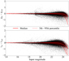 |
Fig. 3 Difference between the output and input magnitude vs. input magnitude in g (top) and i (bottom) filters derived from AS tests for tile 3_17. The solid red line marks the median of the distributions, while the dashed lines indicate the fifth and 95th percentiles of the distributions. |
Age bins used for the SFH analysis and their durations.
3.1 Distance and extinction
We adapted the libraries of partial models to match the characteristics of each observed tile. For the distance, we initially assumed a linear gradient between the distance moduli of the LMC and SMC found in the literature, −18.47 mag (Pietrzynski et al. 2019) and ~18.97 mag (Graczyk et al. 2020), respectively. For the Galactic foreground reddening correction, we adopted E(B-V) values from the SFD reddening map (Schlafly & Finkbeiner 2011). We employed the Cardelli et al. (1989) extinction law, assuming a normal total-to-selective extinction value of RV = 3.1. To account for differential reddening within each region, we determined a unique reddening value for every synthetic star that was randomly selected from a Gaussian distribution, centred on the median E(B-V) and its spread for that particular region. Additionally, we applied a stronger reddening correction for younger stars (≤75 Myr). For these stars, the E(B-V) value was twice that applied to older stars. The final parameters chosen in the analysis of each tile are listed in Table 3. The extinction towards the Bridge is generally low, with a median E(B-V) value of −0.06 mag, in line with previous studies on this low dust region (Wagner-Kaiser & Sarajedini 2017). The extinction increases slightly towards the dustier outskirts of the LMC.
3.2 Photometric errors and incompleteness
Our partial models were then convolved with the incompleteness and photometric errors derived from the AS tests described in Section 2.3. The completeness limit defines the faintest magnitude at which we can confidently detect and measure objects in our observed field. Ideally, we aim for a limit that allows us to observe main-sequence (MS) stars down to 0.8 M⊙, as these stars have lifetimes longer than the age of the universe tracing SF across cosmic time. The completeness distribution in the CMD determines the weight assigned to each synthetic star. Meanwhile, photometric errors, estimated as the difference between the recovered and input magnitudes, are used to model the uncertainty across the full magnitude range. An appropriate photometric error is assigned to each synthetic star based on its position in the CMD. To this purpose, we applied a bilinear interpolation scheme that displaces each synthetic star in both colour and magnitude, considering the error distribution from adjacent CMD cells. This approach ensures a realistic representation of observational uncertainties in our final models.
Summary of the parameters used in the recovery of the SFH of each tile in the Magellanic Bridge.
3.3 Milky Way contamination
To correct for MW contamination in our CMDs, we used a secondary field located near the Bridge (Figure 4). This field4 was observed as part of the Yes, Magellanic Clouds Again survey (YMCA; Gatto et al. 2024), a survey of the outskirts of the MCs from the same instrument, same filters, and with similar observing strategy. The stellar density of the LMC drops abruptly beyond approximately 9° from its centre and from ∼6° from the SMC centre (Gatto et al. 2024). We selected tile 4_14 due to its relatively large distance from both the LMC (∼13.4°) and the SMC (∼9.2°), where the CMD is expected to be dominated by MW foreground stars (third panel, third row of Figure 9 in Gatto et al. (2024). This YMCA tile also shares a similar Galactic latitude with the analysed regions. We excluded the presence of gradients in the colour distribution of MW contaminants across our Galactic latitude range using TRILEGAL (Girardi et al. 2005, 2012) to simulate MW stellar counts across the range −44° ≤ b ≤ −38°, resulting in no sensible variation (see Figure 5). An alternative approach would have been to generate the synthetic foreground CMD with TRILEGAL for fields centred on the analysed tiles. We also plot the Gaia DR3 data distribution for a region centred at l = 298° deg and b = −44° deg, for reference. In Appendix A, we present the comparison between the recovered SFH and the residuals obtained using the two approaches. We found that the synthetic MW model generated with TRILEGAL produces significantly higher residuals, making it less effective in modelling contamination compared to secondary field observations. In light of these tests, we chose to use the YMCA tile as a representative case of MW contamination in all analysed CMDs. In the end, The additional MW model is added to our partial model library and we incorporate it into the final synthetic population as described in the following paragraph.
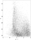 |
Fig. 4 CMD of the tile 4_14 from the YMCA survey, used to model the MW contamination in our analysis. |
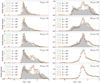 |
Fig. 5 Stellar density distribution for Galactic longitude l = 289° across different latitude bins (−44° ≤ b ≤ −38°). Each panel displays the normalized GBP - GRP colour distribution for different magnitude intervals sourced from the TRILEGAL Galactic model (Girardi et al. 2005, 2012). The Gaia EDR3 distributions at b = −42° are plotted in gray. |
3.4 Finding the best-fit model
The next step is to construct a synthetic representation of a stellar population with a given SFH and age-metallicity relation (AMR) with a combination of the partial models. To quantify the similarity between a synthetic model and the observational data, we divide the CMDs into a grid of magnitude and colour bins, then, for each bin, we compare the predicted and observed star counts. Once binned, the CMDs become Hess diagrams, where the third axis represents the number of stars inside each colour-magnitude cell i. The Hess diagram of any synthetic model is therefore a linear combination of the N × M Hess diagrams of the partial CMDs:
 (1)
(1)
where MODi is the number of stars in cell i in the synthetic model, pi(j, k) is the number of stars into cell i associated with the partial model of age step j and metallicity step k, and w(j, k) are the weighting coefficients associated to each partial model in the linear combination. The foreground model is added to the library of partial CMDs to estimate the contribution of sources of the MW. Thus, when we create the synthetic population, Equation (1) becomes
 (2)
(2)
where wMW is the weight associated with the MW model and fi are the star-counts in bin i of the foreground CMD. The statistical similarity between two Hess diagrams is evaluated with a Poisson based likelihood function, of the form
 (3)
(3)
where obsi represent the number of star-counts in cell i in the data. The most likely SFH is determined by finding the combination of partial models that minimize the likelihood function of the residuals. To simplify the parameter space, in each tile, we consider populations with one value of distance modulus and mean extinction. We assess the sensitivity of the fit to these parameters by systematically varying them and repeating the SFH recovery. To optimize the comparison between models and observations, we employ a variable cell width in the CMD grid: finer bins where the CMD is densely populated; coarser bins where the stellar density is lower or models are more uncertain. The SFERA algorithm determines the optimal set of weighting parameters w(j, k) that generate the best-fitting synthetic stellar population. For each age step tj and metallicity step Zk, the corresponding partial model of mass M(j, k) has an associated weight w(j, k). The total stellar mass formed in the age interval tj is then obtained by summing over all metallicity bins:
 (4)
(4)
where N is the number of metallicity steps. Dividing this mass by the duration of the age interval ∆tj gives the SFR:
 (5)
(5)
Concerning the AMR, the mean metallicity for each age step tj is computed by summing the metallicity values of partial models, weighted by the ratio of their masses to the total mass of the best-fit model at that age:
 (6)
(6)
We repeated this procedure over all ages covered by the partial models to estimate the AMR.
To assess the uncertainty around the best-fit model, we employed a bootstrapping technique, using 25 bootstrap resamplings per analysed tile. After recovering the SFH from each bootstrap, we calculate the confidence interval around the solution as the fifth and 95th percentiles of the parameters’ distribution. The goodness of fit can be visually evaluated as the difference between the Hess diagrams of the observed data and the best-fit model. Ideally, the residuals should not exhibit systematic patterns but rather appear as structureless noise.
4 Results
We present here the best-fit SFH for all tiles in the Bridge. As an example, Fig. 6 (top panels) displays the observational data for tile 2_11 alongside the best-fit synthetic models from PARSEC-COLIBRI and BaSTI. In the bottom panel, the figure also presents the residuals, the observed and recovered luminosity functions and colour distributions. The algorithm effectively captures the overall structure of the observed Hess diagram, successfully replicating all the characteristics of the observed CMDs, albeit with some remaining discrepancies in some regions, such as the incorrect recovery of the red clump (RC) morphology in tile 3_20 (see Figure A.3). These residuals may be due to the theoretical modelling uncertainties of advanced stages of stellar evolution, particularly those involving the intricate interplay of physical processes that are not yet fully understood (such as late-phase stellar winds, convection, and mass loss). Nevertheless, 90% of the residuals fall within ±1 σ. In Figure 7, we compare the SFHs obtained using the PARSEC-COLIBRI and BaSTI models in tile 2_11. The results from the two stellar evolutionary libraries are, overall, in very good agreement, within the error bars, and this is also seen in almost all other tiles.
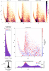 |
Fig. 6 CMDs of the observed data (top left) of tile 2_11 compared with the best-fit synthetic model from PARSEC-COLIBRI (top centre) and BaSTI (top right) stellar isochrones. In the plot at the bottom we show the residuals and the comparison between the observed and recovered luminosity functions and colour distributions, as well as the distribution of residuals from the PARSEC-COLIBRI models. |
4.1 The SFH of the Bridge
Figure 8 provides a comprehensive view of the SFH across all the Magellanic Bridge tiles, highlighting significant tile-to-tile variations. Several fields show low recent SF, while a limited number of tiles, those closer to the SMC, display enhanced activity at ages younger than 150 Myr. In Figure 9, it is clear that upper main-sequence (UMS) stars (g < 20 and g - i < -0.2) are concentrated towards the western side of the Bridge, closer to the SMC. While a broad correspondence between young stellar concentrations and regions of high HI column density is observed in tiles immediately adjacent to the SMC, this correlation becomes weaker within the Bridge itself.5.
In particular, tile 3_14 deserves special attention. Unlike neighbouring fields, its SFH shows a continuous rise up to the present time, resulting in a well-populated young MS. This population is clearly visible in its CMD (Figure B.1), which provides sufficient statistics to robustly constrain recent SF. A comparison between the top and bottom panels of Figure 9 shows that the region hosting this concentration of young stars coincides with a local depression in the H I column density, suggesting that the gas may have been recently consumed to fuel the ongoing SF episode. This location corresponds to the ’OGLE Island’ reported by Skowron et al. (2014), a small isolated young population in the Magellanic Bridge. In contrast, the adjacent tiles contain a larger amount of gas but show fewer UMS stars, as evidenced in Fig. B.1, suggesting inhomogeneous star-forming efficiency across small spatial scales in the Bridge. This absence of very young stars beyond RA = 03h (45°) was already noted by Harris (2007), who suggested that it might be linked to the drop in HI surface density below the threshold required to trigger SF (Kennicutt 1989).
The central tiles of the Bridge (3_15, 3_16 and 3_17) do not show evidence for a stellar population younger than −400 Myr. This is reflected both in the corresponding SFHs (note that the maximum y-axis value is significantly lower than in the adjacent regions) and in the paucity of UMS stars in the density map (upper panel of Figure 9). A visual inspection of the CMDs (Figure B.1) further supports this conclusion, as no distinct young MS comparable to that observed in tile 3_14 is detected. Together, these indicators suggest that recent SF in the central Bridge is extremely weak, if present at all.
Assuming a tangential velocity of approximately −80—110 km/s (Zivick et al. 2018; Schmidt et al. 2020; Gaia Collaboration 2021), the young stellar population of the Bridge likely formed in situ or in the nearby regions of the SMC. Given such a velocity, it would not have had sufficient time to migrate more than −8 kpc over such a short timescale. This is consistent with the lower HI gas velocity observed in the Wing, traced by the young, massive stars embedded within it (Murray et al. 2019).
Concerning older populations, we detect a modest amount of ancient (≳8 Gyr) stars in the inter-cloud region, which appear to be uniformly distributed along the Bridge and likely pertain to the halos of the two Clouds. However, in the central parts of the Bridge, the CMDs are dominated by the contamination from MW stars. The absence of clumps in the distribution of RC and red giant branch (RGB) stars (19.5 ≲ g ≲ 22 mag and 0.6 ≲ g -i ≲ 1.2 mag, in the central panel of Figure 9) may imply that the primary outcome of the last pericentric passage was the stripping of gas rather than stars.
In tiles 3_19, 3_20, and 3_21, dominated by the outer LMC population, the SFH shows a dominant old population (>7 Gyr) as well as a distinct peak at ∼2 Gyr. The former is consistent with the oldest SF seen in Harris (2007) close to the LMC (region mb20) and in Ruiz-Lara et al. (2020), while the latter corresponds to a major SF episode found in the global SFH of both Clouds (Massana et al. 2022).
Figure 10 presents the global SFH of the Bridge, obtained by summing the SFHs of the individual tiles for both the stellar models adopted. The dashed lines indicate periods of enhanced SF activity found by Ruiz-Lara et al. (2020), Mazzi et al. (2021) and Massana et al. (2022). Given that the SFR uncertainties in each tile are independent, the total error was calculated as the square root of the sum of the squared individual errors. We found that the Magellanic Bridge hosts ongoing SF, which primarily began approximately 100 Myr ago. The main difference between the two stellar models lies in the amount of SF from 100 Myr ago to the present day, which may reflect differences in how young stellar populations are treated by the two sets of stellar evolution codes and their high-mass limit. For all other epochs, the SFHs derived from the two sets show excellent agreement. The old periods of enhanced SF at ~2 Gyr and ~10 Gyr are consistent with the main features of activity observed in previous works in the literature. Interestingly, the peak at ~2 Gyr may suggest a previous close encounter between the two Clouds at that time, as a similar feature can be found in previous works in the literature in both the SMC and LMC (Ruiz-Lara et al. 2020; Mazzi et al. 2021; Massana et al. 2022). Recent studies (Bica et al. 2020; Oliveira et al. 2023) on the clusters of the Bridge have found different populations: an older, metal-poor group (0.5-6.8 Gyr, [Fe/H] < −0.6 dex) likely stripped from the SMC outskirts, and a younger population (<200 Myr) with significantly higher metallicities (−0.5 < [Fe/H] < −0.1), which likely formed in situ. The well-established peak in the age distribution of star clusters around 2-3 Gyr in both galaxies (Rafelski & Zaritsky 2005; Pieres et al. 2016; Gatto et al. 2020, 2024; Dhanush et al. 2024) provides additional evidence that such an event could have triggered enhanced SF across the Magellanic system. This period likely coincides with the formation epoch of the Magellanic Stream and the arrival of the Clouds into the MW halo (Besla et al. 2012; Lucchini et al. 2020). We estimated the total stellar mass in the Bridge, excluding tiles 3_21, 3_20, 3_19 and 3_18, where the population is almost entirely composed of old LMC stars. For each tile, we calculated the mass from the best-fit solution of each bootstrap run and then took the median of the 25 resulting estimates. Summing over all tiles, we obtain a total mass of M* ~ (5.1 ± 0.2) × 105 M⊙, which lies at the upper end of the of minimum stellar mass range proposed by Oliveira et al. (2023), that is already significantly higher than previous estimates (Harris 2007).
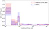 |
Fig. 7 SFH of tile 2_11 recovered with PARSEC-COLIBRI (red) and BaSTI (blue) stellar isochrones. |
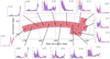 |
Fig. 8 Map of the analysed regions overlaid with the SFH of the individual tiles. The lines connect the location of each tile on the map to its corresponding inset plot, which displays the SFR in unit of 10−4 M⊙ yr−1 resulting from the PARSEC-COLIBRI (red) and BaSTI (blue) stellar evolution libraries as a function of age in Gyr (logarithmic scale). The y-axis limits are independently scaled for each tile to better show the SFH features of each region and the axis labels were omitted for enhanced clarity. The shaded regions represent the fifth and 95th percentile uncertainties of the SFR. |
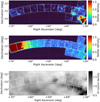 |
Fig. 9 Spatial distribution of UMS stars (top), RGB and RC (centre) and HI gas column density distribution (bottom) from the GASS survey (McClure-Griffiths et al. 2009). |
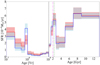 |
Fig. 10 Comparison between the global SFH of the Magellanic Bridge recovered using the PARSEC-COLIBRI (red line) and BaSTI (blue line) stellar models. The dashed pink line indicates a period of intense SF found by Mazzi et al. (2021); the dashed green line indicates the first synchronized SF peak of the MCs found by Massana et al. (2022) and Ruiz-Lara et al. (2020). Notice that the left portion of the abscissa is in logarithmic age scale to better appreciate the details, while the right portion is in linear scale. The shaded area represents the confidence interval of our solution, computed as the fifth and 95th percentiles of the parameters’ distribution. |
4.2 Age-metallicity relation
Regarding the AMR, we did not place any constraints on the SFH recovery algorithm, allowing the metal-content to vary in the range −2 < [Fe/H] < 0 dex. Figure 11 displays the best fits of the AMR for the entire Magellanic Bridge. The metallicities from Equation (6) were averaged for each tile. Each tile’s contribution was weighted by the number of stars above a threshold magnitude, to account for differences in completeness. We highlight that the AMR features at older ages (>1 Gyr) mainly reflect the tiles near the LMC, while the younger populations are dominated by tiles closer to the SMC. Therefore, the overall AMR is not the result of a coherent chemical evolution but rather reflects the mixing of stellar populations originating from different parent systems. Only the youngest stars are likely to have formed in situ within the Bridge. The results from both adopted stellar libraries indicate that the metallicity slowly grew up to approximately 5 Gyr ago, after which the production of metals began to accelerate, up to ~2 Gyr ago. The metallicity values we recovered for stars older than 1 Gyr are systematically lower than those of Carrera et al. (2008b); this discrepancy may be attributed to the fact that they analysed the disk of the LMC and did not reach the periphery of the galaxy.
Although metallicity gradients in dwarf galaxies were once debated, improved observations have now revealed their presence in many systems. Early investigations that did not detect such gradients (e.g. Lee et al. 2006; Bresolin et al. 2009; Cairós et al. 2009) were likely limited by the restricted spatial coverage and sensitivity of available data. Several studies have indeed reported declining metallicity with radius (Dobbie et al. 2014; Pilyugin et al. 2015; Annibali et al. 2015, 2017, 2019; Choudhury et al. 2021; Taibi et al. 2022; Li et al. 2024). Recent studies based on the analysis of many high resolution spectra have clearly detected metallicity gradients in both the LMC and SMC (Povick et al. 2025a,b; Omkumar et al. 2025); the lower metallicities found in this work could be influenced by these radial trends. Figure 12 shows that the AMR lies between the typical SMC and LMC values and broadly follows the expected spatial trend from the SMC side towards the LMC along the Bridge. The metallic-ity decreases towards SMC-side regions of the Bridge; however, the uncertainties are larger at these epochs because of the generally low star-formation activity in these regions. In addition, the metallicities derived from photometry are subject to the well-known age-metallicity degeneracy, which further increases the uncertainty.
We find that the young stellar population (left portion of Figure 11) have [Fe/H]~ −0.6 dex, similar to the results of Rubele et al. (2018) in the SMC, suggesting that the material forming the young population of the Bridge was stripped primarily from the SMC during the last close encounter between the Clouds. Interestingly, a metallicity dip has also been reported for clusters around −200 Myr ago, with metallicity decreasing from −0.25 to −0.55 dex (Oliveira et al. 2023), suggesting a second infall of metal-poor gas. The stellar metallicity we observe is higher than that measured for three O-type stars in the eastern outskirts of the SMC (Ramachandran et al. 2021). This discrepancy could arise due to inefficient mixing from stellar winds and supernovae in the Bridge, combined with additional chemical inhomogeneities caused by the accretion of metal-poor gas by interactions between the MCs.
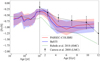 |
Fig. 11 Global AMR of the Magellanic Bridge found using the PADOVA-COLIBRI (red line) and BaSTI (blue line) stellar models. The left portion of the abscissa is in logarithmic scale to better appreciate the details, while the right portion is in linear scale. The shaded area represents the confidence interval of our solution, computed as the fifth and 95th percentiles of the parameters’ distribution. The dashed green line marks the global AMR of the SMC obtained by Rubele et al. (2018), while the dashed black line represents the AMR of the LMC from Carrera et al. (2008b). |
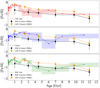 |
Fig. 12 AMR for the three observed regions, with the top, central, and bottom panels representing the LMC-side, central, and SMC-side regions, respectively. Each point corresponds to the mean metallicity within an age bin, with horizontal error bars showing the bin width. The black diamonds and orange hexagons indicate spectroscopic measurements for the SMC (Carrera et al. 2008a) and LMC (Carrera et al. 2008b), respectively. |
4.3 Star formation efficiency in the Bridge: Testing the Kennicutt-Schmidt relation
To investigate the efficiency of SF in the Bridge, we compared the observed gas and star formation rate (SFR) surface densities. This allows us to test whether the Bridge follows the same scaling laws observed in other galaxies, or whether its low density, low metallicity, and tidally disturbed environment lead to a reduced efficiency in forming stars. The key empirical relationship describing the conversion of gas into stars is the Kennicutt-Schmidt (KS) law (Kennicutt 1989, 1998), which expresses a power-law correlation between the SFR surface density (∑SFR) and the gas mass surface density (Σgas) in galaxies:
 (7)
(7)
where n ~ 1.0-1.4 for a wide range of galaxy types (Kennicutt 1989; de los Reyes & Kennicutt 2019; Sun et al. 2023). The classical KS relation tends to hold for massive galaxies but often deviates for gas-rich lower-mass dwarf galaxies, especially metal-poor ones such as the MCs. This deviation depends on the dominant gas phase (atomic vs. molecular), the galactic environment, and the spatial scales considered. The Krumholz et al. (2009) model (KMT09) refines the KS relation as
 (8)
(8)
where tdep is the molecular gas depletion time and fH2 is the molecular gas fraction, determined by the balance between the dissociation and the formation of molecules on dust grains’ surfaces. In the fH2 (Σgas, c, Z′) parameter, KMT09 accounts for the gas metallicity (Z′) and the degree of gas clumping (c). Metallicity affects dust abundance, which in turn influences H2 formation and far-ultraviolet (FUV) radiation field shielding. Gas clumping, on the other hand, directly impacts local density and shielding. The dependence on these factors leads to a characteristic S-shaped curve with an atomic-dominated regime for low Σgas, where ΣSFR is significantly suppressed and deviates strongly from the classical KS relation. Therefore, KMT09 provides a more physically motivated description of the SF law, explaining why simple power-law relations often fail to capture the observed variations in diverse galactic environments.
To determine Σgas, we utilized the HI4PI survey data (HI4PI Collaboration 2016). The HI4PI survey provides all-sky maps of HI column density (NHI) in units of square centimetre. We averaged the individual NHI values within each of the studied regions and converted the average HI column density into a surface density ΣHI:
 (9)
(9)
where mH = 1.673 × 10⁻²⁴ g is the mass of a hydrogen atom. This simplifies to approximately NHI × 8.02 × 10⁻²¹ M⊙ pc−2. In absence of molecular hydrogen (H2) column density maps in the literature, we assumed a fixed 10% contribution from H2 to the total gas mass, consistent with values for dwarf galaxies and outer galactic disks where H I often dominates (Bolatto et al. 2011; Di Teodoro et al. 2019) and the molecular fraction is typically low (∼ 10-20%). Finally, we compared the gas column density with ΣSFR, calculated as the SFR in the most recent age bin of each tile divided by the tile area (∼1 kpc). As shown in Figure 13, ΣSFR follows the slope expected in the KMT09 theoretical framework. We only show the results from the PARSEC-COLIBRI library for clarity, and the results with the BaSTI models are similar. Our study extends this established trend to even lower values of ΣHI, in a regime where molecular gas formation is less efficient. The observed trend in our data aligns well with the trend observed by Bolatto et al. (2011), who examined the SF efficiency in the SMC.
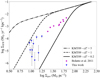 |
Fig. 13 SF law in the Magellanic Bridge (blue triangles) in comparison with the data by Bolatto et al. (2011) (magenta filled circles) and curves of the KMT09 models (adapted from the same authors) for different values of the cZ′ parameter (the product of the gas metallicity Z′ and the degree of gas clumping c) indicated by the dash-dotted, dashed, and solid lines. |
5 Conclusions
In this work, we analysed the SFH of the entire Magellanic Bridge, covering a total area of 14 deg2 using data from the STEP Survey. We employed the ‘synthetic CMD’ method and derived the best-fitting SFH using the genetic algorithm SFERA. Our library of partial models covered the whole Hubble time and a metallicity range of −2.0 ≤ [Fe/H] ≤ 0. To explore systematic differences, we used two distinct sets of stellar evolutionary models: PARSEC-COLIBRI and BaSTI. For each analysed tile, we assumed a distance based on a linear trend between the distances of the LMC and the SMC. Extinction corrections were derived from the SFD extinction map. Thanks to the high photometric accuracy of the STEP survey, we were able to map the spatial distribution of stellar ages and trace the metallicity evolution across the Magellanic Bridge with high temporal resolution. Our findings significantly extend previous analyses, covering a region more than three times larger than the most comprehensive SFH study of the Bridge by Harris (2007). The key results include:
The young stellar population is more evident in the region of the Magellanic Bridge closer to the SMC. The solutions from both PARSEC-COLIBRI and BaSTI models consistently predict low SF activity before ∼ 100 Myr ago, when SF was ignited and continued to rise up to the present day. This time frame aligns with predictions from dynamical models for the Magellanic Bridge’s formation, and the metallicity of stars from this event matches that of the SMC;
A very old stellar population originating in the LMC is observed in the three tiles closer to the LMC. These periods of enhanced SF are consistent with peaks found in previous studies in the LMC (∼10 Gyr) and in both MCs (∼2.1 Gyr) (Rubele et al. 2018; Ruiz-Lara et al. 2020; Mazzi et al. 2021);
We observe only minimal differences between the SFHs recovered using the PARSEC-COLIBRI and BaSTI stellar libraries, except for the height of the SFR peak at 100 Myr, which arises from different physical assumptions in the PARSEC-COLIBRI and BaSTI stellar models. These differences are most pronounced for the young, intermediate-mass stars that dominate a 100 Myr population and thus are probably related to the treatment of core convective overshooting, mass loss, and post-MS evolution. This leads to modeldependent stellar luminosities, which in turn affects the inferred number of stars required to match the observational data;
The metallicity evolution at old ages follows the trend observed in the LMC, though it is systematically lower. This may be due to the fact that we observe material originating from the outer regions of the LMC, as metallicity is expected to decrease with galactocentric radius. In the past 400 Myr, the AMR closely matches the global AMR of the SMC, further supporting the scenario that most of the material forming the Bridge was stripped from the SMC;
The present-day metallicity is [Fe/H] ~ −0.6 dex, higher than that derived for three O-type stars in the SMC’s eastern outskirts (Ramachandran et al. 2021). This may be due to chemical inhomogeneities caused by previous interactions between the MCs, as well as inefficient mixing processes from stellar winds and supernovae within the Bridge;
We estimated the total stellar mass formed in the Magellanic Bridge, excluding those dominated by old LMC stars. The resulting total mass across ∼10 deg2 is M* ∼ (5.1 ± 0.2) ∙ 105 M⊙, higher than previous estimates (Harris 2007; Oliveira et al. 2023);
We used HI4PI survey data to estimate the Σgas in the Bridge and compared it with our resulting ΣSFR. We see good agreement with the theoretical framework of the KMT09 model, extending the trend observed by Bolatto et al. (2011) to a regime where the formation of molecular gas and, therefore, SF is less efficient.
Our findings suggest the recent collision between the SMC and LMC likely occurred no more than a few tens of megayears before the peak we found 100 Myr ago. This coincides with the predicted time when the SMC crossed the LMC’s disk plane (Besla et al. 2013; Choi et al. 2022). Our results can help place constraints on models of the MCs’ interaction history and better understand the tidal origin of the stellar populations in the Bridge.
Data availability
Full Table 1 is available at the CDS via https://cdsarc.cds.unistra.fr/viz-bin/cat/J/A+A/709/A10.
Acknowledgements
We thank our anonymous referee for the insightful comments and suggestions that helped us improve the paper. This research has used the SIMBAD database operated at CDS, Strasbourg, France. We acknowledge funding from: INAF GO-GTO grant 2023 “C-MetaLL - Cepheid metallicity in the Leavitt law” (P.I. V. Ripepi); PRIN MUR 2022 project (code 2022ARWP9C) ‘Early Formation and Evolution of Bulge and Halo (EFEBHO),’ PI: Marconi, M., funded by the European Union - Next Generation EU; Large Grant INAF 2023 MOVIE (P.I. M. Marconi). This research has made use of the APASS database, located at the AAVSO web site. Funding for APASS has been provided by the Robert Martin Ayers Sciences Fund. M.B. acknowledges the financial support by the Italian MUR through the grant PRIN 2022LLP8TK_001 assigned to the project LEGO - Reconstructing the building blocks of the Galaxy by chemical tagging (P.I. A. Mucciarelli), funded by the European Union - NextGenera-tionEU. M.G. acknowledges “Partecipazione LSST - Large Synoptic Survey Telescope (ref. A. Fontana)” (Ob. Fu.: 1.05.03.06).
References
- Annibali, F., Tosi, M., Romano, D., et al. 2017, ApJ, 843, 20 [Google Scholar]
- Annibali, F., La Torre, V., Tosi, M., et al. 2019, MNRAS, 482, 3892 [NASA ADS] [CrossRef] [Google Scholar]
- Annibali, F., Tosi, M., Pasquali, A., et al. 2015, AJ, 150, 143 [NASA ADS] [CrossRef] [Google Scholar]
- Aparicio, A. & Hidalgo, S. L. 2009, AJ, 138, 558 [NASA ADS] [CrossRef] [Google Scholar]
- Bagheri, G., Cioni, M. R. L., & Napiwotzki, R. 2013, A&A, 551, A78 [NASA ADS] [CrossRef] [EDP Sciences] [Google Scholar]
- Belokurov, V. A., & Erkal, D. 2019, MNRAS, 482, L9 [Google Scholar]
- Besla, G., Kallivayalil, N., Hernquist, L., et al. 2007, ApJ, 668, 949 [Google Scholar]
- Besla, G., Kallivayalil, N., Hernquist, L., et al. 2011, in American Astronomical Society Meeting Abstracts, 217, American Astronomical Society Meeting Abstracts #217, 424.04 [Google Scholar]
- Besla, G., Kallivayalil, N., Hernquist, L., et al. 2012, MNRAS, 421, 2109 [Google Scholar]
- Besla, G., Hernquist, L., & Loeb, A. 2013, MNRAS, 428, 2342 [NASA ADS] [CrossRef] [Google Scholar]
- Besla, G., Martinez-Delgado, D., van der Marel, R. P., et al. 2016, ApJ, 825, 20 [Google Scholar]
- Bica, E., Westera, P., Kerber, L. d. O., et al. 2020, AJ, 159, 82 [Google Scholar]
- Bolatto, A. D., Leroy, A. K., Jameson, K., et al. 2011, ApJ, 741, 12 [CrossRef] [Google Scholar]
- Bresolin, F., Gieren, W., Kudritzki, R.-P., et al. 2009, ApJ, 700, 309 [NASA ADS] [CrossRef] [Google Scholar]
- Bressan, A., Marigo, P., Girardi, L., et al. 2012, MNRAS, 427, 127 [NASA ADS] [CrossRef] [Google Scholar]
- Cairós, L. M., Caon, N., Papaderos, P., et al. 2009, ApJ, 707, 1676 [CrossRef] [Google Scholar]
- Capaccioli, M., & Schipani, P. 2011, The Messenger, 146, 2 [NASA ADS] [Google Scholar]
- Cardelli, J. A., Clayton, G. C., & Mathis, J. S. 1989, ApJ, 345, 245 [Google Scholar]
- Carrera, R., Gallart, C., Aparicio, A., et al. 2008a, AJ, 136, 1039 [Google Scholar]
- Carrera, R., Gallart, C., Hardy, E., Aparicio, A., & Zinn, R. 2008b, AJ, 135, 836 [NASA ADS] [CrossRef] [Google Scholar]
- Charbonneau, P. 1995, ApJS, 101, 309 [Google Scholar]
- Choi, Y., Nidever, D. L., Olsen, K., et al. 2018, ApJ, 866, 90 [Google Scholar]
- Choi, Y., Olsen, K. A. G., Besla, G., et al. 2022, ApJ, 927, 153 [NASA ADS] [CrossRef] [Google Scholar]
- Choudhury, S., de Grijs, R., Bekki, K., et al. 2021, MNRAS, 507, 4752 [CrossRef] [Google Scholar]
- Cignoni, M., & Tosi, M. 2010, Adv. Astron., 2010, 158568 [CrossRef] [Google Scholar]
- Cignoni, M., Sabbi, E., Nota, A., et al. 2009, AJ, 137, 3668 [NASA ADS] [CrossRef] [Google Scholar]
- Cignoni, M., Cole, A. A., Tosi, M., et al. 2012, ApJ, 754, 130 [NASA ADS] [CrossRef] [Google Scholar]
- Cignoni, M., Cole, A. A., Tosi, M., et al. 2013, ApJ, 775, 83 [Google Scholar]
- Cignoni, M., Sabbi, E., van der Marel, R. P., et al. 2015, ApJ, 811, 76 [Google Scholar]
- Cioni, M. R. L., Clementini, G., Girardi, L., et al. 2011, A&A, 527, A116 [CrossRef] [EDP Sciences] [Google Scholar]
- Cioni, M.-R. L., Cross, N. J. G., Ripepi, V., et al. 2025, A&A, 699, A300 [NASA ADS] [CrossRef] [EDP Sciences] [Google Scholar]
- Cohen, R. E., McQuinn, K. B. W., Murray, C. E., et al. 2024a, ApJ, 975, 43 [Google Scholar]
- Cohen, R. E., McQuinn, K. B. W., Murray, C. E., et al. 2024b, ApJ, 975, 42 [Google Scholar]
- Cullinane, L. R., Mackey, A. D., Da Costa, G. S., et al. 2022, MNRAS, 510, 445 [Google Scholar]
- De Leo, M., Carrera, R., Noël, N. E. D., et al. 2020, MNRAS, 495, 98 [Google Scholar]
- de los Reyes, M. A. C., & Kennicutt, Jr., R. C. 2019, ApJ, 872, 16 [NASA ADS] [CrossRef] [Google Scholar]
- Demers, S., & Irwin, M. J. 1991, A&AS, 91, 171 [Google Scholar]
- Dhanush, S. R., Subramaniam, A., Nayak, P. K., & Subramanian, S. 2024, MNRAS, 528, 2274 [Google Scholar]
- Di Teodoro, E. M., McClure-Griffiths, N. M., De Breuck, C., et al. 2019, ApJ, 885, L32 [NASA ADS] [CrossRef] [Google Scholar]
- Diaz, J. D., & Bekki, K. 2012, ApJ, 750, 36 [Google Scholar]
- Dobbie, P. D., Cole, A. A., Subramaniam, A., & Keller, S. 2014, MNRAS, 442, 1680 [NASA ADS] [CrossRef] [Google Scholar]
- Dolphin, A. 1997, New A, 2, 397 [NASA ADS] [CrossRef] [Google Scholar]
- Dolphin, A. E. 2002, MNRAS, 332, 91 [NASA ADS] [CrossRef] [Google Scholar]
- Dolphin, A. E., Walker, A. R., Hodge, P. W., et al. 2001, ApJ, 562, 303 [NASA ADS] [CrossRef] [Google Scholar]
- D’Onghia, E., & Fox, A. J. 2016, ARA&A, 54, 363 [Google Scholar]
- El Youssoufi, D., Cioni, M.-R. L., Bell, C. P. M., et al. 2019, MNRAS, 490, 1076 [NASA ADS] [CrossRef] [Google Scholar]
- Fukugita, M., Ichikawa, T., Gunn, J. E., et al. 1996, AJ, 111, 1748 [Google Scholar]
- Gaia Collaboration (Luri, X., et al.) 2021, A&A, 649, A7 [EDP Sciences] [Google Scholar]
- Gardiner, L. T., & Noguchi, M. 1996, MNRAS, 278, 191 [Google Scholar]
- Gatto, M., Ripepi, V., Bellazzini, M., et al. 2020, MNRAS, 499, 4114 [Google Scholar]
- Gatto, M., Ripepi, V., Bellazzini, M., et al. 2021, MNRAS, 507, 3312 [NASA ADS] [CrossRef] [Google Scholar]
- Gatto, M., Ripepi, V., Bellazzini, M., et al. 2022, ApJ, 931, 19 [Google Scholar]
- Gatto, M., Ripepi, V., Bellazzini, M., et al. 2024, A&A, 690, A164 [NASA ADS] [CrossRef] [EDP Sciences] [Google Scholar]
- Girardi, L., Groenewegen, M. A. T., Hatziminaoglou, E., & da Costa, L. 2005, A&A, 436, 895 [NASA ADS] [CrossRef] [EDP Sciences] [Google Scholar]
- Girardi, L., Barbieri, M., Groenewegen, M. A. T., et al. 2012, in Astrophysics and Space Science Proceedings, 26, Red Giants as Probes of the Structure and Evolution of the Milky Way, eds. A. Miglio, J. Montalbán, & A. Noels, 165 [Google Scholar]
- Graczyk, D., Pietrzynski, G., Thompson, I. B., et al. 2020, ApJ, 904, 13 [Google Scholar]
- Grado, A., Capaccioli, M., Limatola, L., & Getman, F. 2012, Mem. Soc. Astron. Ital. Suppl., 19, 362 [NASA ADS] [Google Scholar]
- Grebel, E. K., Gallagher, III, J. S., & Harbeck, D. 2003, AJ, 125, 1926 [NASA ADS] [CrossRef] [Google Scholar]
- Guglielmo, M., Lewis, G. F., & Bland-Hawthorn, J. 2014, MNRAS, 444, 1759 [Google Scholar]
- Gunn, J. E., Carr, M., Rockosi, C., et al. 1998, AJ, 116, 3040 [NASA ADS] [CrossRef] [Google Scholar]
- Harris, J. 2007, ApJ, 658, 345 [Google Scholar]
- Harris, J., & Zaritsky, D. 2004, AJ, 127, 1531 [NASA ADS] [CrossRef] [Google Scholar]
- Harris, J., & Zaritsky, D. 2009, AJ, 138, 1243 [NASA ADS] [CrossRef] [Google Scholar]
- Haschke, R., Grebel, E. K., & Duffau, S. 2012, AJ, 144, 106 [NASA ADS] [CrossRef] [Google Scholar]
- Henden, A. A., Levine, S., Terrell, D., & Welch, D. L. 2015, in American Astronomical Society Meeting Abstracts, 225, American Astronomical Society Meeting Abstracts #225, 336.16 [Google Scholar]
- Hernandez, X., Valls-Gabaud, D., & Gilmore, G. 1999, MNRAS, 304, 705 [NASA ADS] [CrossRef] [Google Scholar]
- HI4PI Collaboration (Ben Bekhti, N., et al.) 2016, A&A, 594, A116 [NASA ADS] [CrossRef] [EDP Sciences] [Google Scholar]
- Hidalgo, S. L., Pietrinferni, A., Cassisi, S., et al. 2018, ApJ, 856, 125 [Google Scholar]
- Hindman, J. V., Kerr, F. J., & McGee, R. X. 1963, Austr. J. Phys., 16, 570 [Google Scholar]
- Holtzman, J. A., Gallagher, III, J. S., Cole, A. A., et al. 1999, AJ, 118, 2262 [Google Scholar]
- Irwin, M. J., Kunkel, W. E., & Demers, S. 1985, Nature, 318, 160 [Google Scholar]
- Irwin, M. J., Demers, S., & Kunkel, W. E. 1990, AJ, 99, 191 [NASA ADS] [CrossRef] [Google Scholar]
- Jacyszyn-Dobrzeniecka, A. M., Skowron, D. M., Mróz, P., et al. 2016, Acta Astron., 66, 149 [NASA ADS] [Google Scholar]
- Jacyszyn-Dobrzeniecka, A. M., Mróz, P., Kruszynska, K., et al. 2020a, ApJ, 889, 26 [Google Scholar]
- Jacyszyn-Dobrzeniecka, A. M., Soszynski, I., Udalski, A., et al. 2020b, ApJ, 889, 25 [Google Scholar]
- Kallivayalil, N., van der Marel, R. P., & Alcock, C. 2006a, ApJ, 652, 1213 [NASA ADS] [CrossRef] [Google Scholar]
- Kallivayalil, N., van der Marel, R. P., Alcock, C., et al. 2006b, ApJ, 638, 772 [NASA ADS] [CrossRef] [Google Scholar]
- Kennicutt, Jr., R. C. 1989, ApJ, 344, 685 [CrossRef] [Google Scholar]
- Kennicutt, Jr., R. C. 1998, ApJ, 498, 541 [Google Scholar]
- Kroupa, P. 2001, MNRAS, 322, 231 [NASA ADS] [CrossRef] [Google Scholar]
- Krumholz, M. R., McKee, C. F., & Tumlinson, J. 2009, ApJ, 699, 850 [NASA ADS] [CrossRef] [Google Scholar]
- Kuijken, K. 2011, The Messenger, 146, 8 [NASA ADS] [Google Scholar]
- Laporte, C. F. P., Gómez, F. A., Besla, G., Johnston, K. V., & Garavito-Camargo, N. 2018, MNRAS, 473, 1218 [NASA ADS] [CrossRef] [Google Scholar]
- Lee, H., Skillman, E. D., & Venn, K. A. 2006, ApJ, 642, 813 [Google Scholar]
- Li, Y., Jiang, B., & Ren, Y. 2024, AJ, 167, 123 [Google Scholar]
- Lucchini, S. 2024, Ap&SS, 369, 114 [Google Scholar]
- Lucchini, S., D’Onghia, E., Fox, A. J., et al. 2020, Nature, 585, 203 [CrossRef] [Google Scholar]
- Lucchini, S., D’Onghia, E., & Fox, A. J. 2021, ApJ, 921, L36 [NASA ADS] [CrossRef] [Google Scholar]
- Marigo, P., Girardi, L., Bressan, A., et al. 2017, ApJ, 835, 77 [Google Scholar]
- Massana, P., Ruiz-Lara, T., Noël, N. E. D., et al. 2022, MNRAS, 513, L40 [CrossRef] [Google Scholar]
- Mastropietro, C., Moore, B., Mayer, L., Wadsley, J., & Stadel, J. 2005, MNRAS, 363, 509 [Google Scholar]
- Mathewson, D. S., Cleary, M. N., & Murray, J. D. 1974, ApJ, 190, 291 [NASA ADS] [CrossRef] [Google Scholar]
- Mazzi, A., Girardi, L., Zaggia, S., et al. 2021, MNRAS, 508, 245 [NASA ADS] [CrossRef] [Google Scholar]
- McClure-Griffiths, N. M., Pisano, D. J., Calabretta, M. R., et al. 2009, ApJS, 181, 398 [NASA ADS] [CrossRef] [Google Scholar]
- McConnachie, A. W. 2012, AJ, 144, 4 [Google Scholar]
- Meschin, I., Gallart, C., Aparicio, A., et al. 2014, MNRAS, 438, 1067 [Google Scholar]
- Moore, B., Ghigna, S., Governato, F., et al. 1999, ApJ, 524, L19 [Google Scholar]
- Murai, T., & Fujimoto, M. 1980, PASJ, 32, 581 [NASA ADS] [Google Scholar]
- Murray, C. E., Peek, J. E. G., Di Teodoro, E. M., et al. 2019, ApJ, 887, 267 [Google Scholar]
- Nidever, D. L., Majewski, S. R., Butler Burton, W., & Nigra, L. 2010, ApJ, 723, 1618 [NASA ADS] [CrossRef] [Google Scholar]
- Nidever, D. L., Majewski, S. R., Burton, W., et al. 2013a, in American Astronomical Society Meeting Abstracts, 221, American Astronomical Society Meeting Abstracts #221, 404.04 [Google Scholar]
- Nidever, D. L., Monachesi, A., Bell, E. F., et al. 2013b, ApJ, 779, 145 [Google Scholar]
- Nidever, D. L., Olsen, K., Walker, A. R., et al. 2017, AJ, 154, 199 [Google Scholar]
- Oliveira, R. A. P., Maia, F. F. S., Barbuy, B., et al. 2023, MNRAS, 524, 2244 [NASA ADS] [CrossRef] [Google Scholar]
- Omkumar, A. O., Cioni, M.-R. L., Subramanian, S., et al. 2025, A&A, 700, A74 [NASA ADS] [CrossRef] [EDP Sciences] [Google Scholar]
- Pardy, S. A., D’Onghia, E., & Fox, A. J. 2018, ApJ, 857, 101 [NASA ADS] [CrossRef] [Google Scholar]
- Pieres, A., Santiago, B., Balbinot, E., et al. 2016, MNRAS, 461, 519 [NASA ADS] [CrossRef] [Google Scholar]
- Pietrzynski, G., Graczyk, D., Gallenne, A., et al. 2019, Nature, 567, 200 [NASA ADS] [CrossRef] [Google Scholar]
- Pilyugin, L. S., Grebel, E. K., & Zinchenko, I. A. 2015, MNRAS, 450, 3254 [CrossRef] [Google Scholar]
- Povick, J. T., Nidever, D. L., Majewski, S. R., et al. 2025a, MNRAS, 544, 457 [Google Scholar]
- Povick, J. T., Nidever, D. L., Massana, P., et al. 2025b, MNRAS, 544, 430 [Google Scholar]
- Putman, M. E., Gibson, B. K., Staveley-Smith, L., et al. 1998, Nature, 394, 752 [Google Scholar]
- Putman, M. E., Staveley-Smith, L., Freeman, K. C., Gibson, B. K., & Barnes, D. G. 2003, ApJ, 586, 170 [NASA ADS] [CrossRef] [Google Scholar]
- Rafelski, M., & Zaritsky, D. 2005, AJ, 129, 2701 [NASA ADS] [CrossRef] [Google Scholar]
- Ramachandran, V., Oskinova, L. M., & Hamann, W. R. 2021, A&A, 646, A16 [NASA ADS] [CrossRef] [EDP Sciences] [Google Scholar]
- Richter, P., Fox, A. J., Wakker, B. P., et al. 2013, ApJ, 772, 111 [Google Scholar]
- Ripepi, V., Cignoni, M., Tosi, M., et al. 2014, MNRAS, 442, 1897 [NASA ADS] [CrossRef] [Google Scholar]
- Ripepi, V., Cioni, M.-R. L., Moretti, M. I., et al. 2017, MNRAS, 472, 808 [Google Scholar]
- Rubele, S., Pastorelli, G., Girardi, L., et al. 2018, MNRAS, 478, 5017 [NASA ADS] [CrossRef] [Google Scholar]
- Ruiz-Lara, T., Gallart, C., Monelli, M., et al. 2020, A&A, 639, L3 [EDP Sciences] [Google Scholar]
- Sabbi, E., Gallagher, J. S., Tosi, M., et al. 2009, ApJ, 703, 721 [NASA ADS] [CrossRef] [Google Scholar]
- Schlafly, E. F., & Finkbeiner, D. P. 2011, ApJ, 737, 103 [Google Scholar]
- Schmidt, T., Cioni, M.-R. L., Niederhofer, F., et al. 2020, A&A, 641, A134 [NASA ADS] [CrossRef] [EDP Sciences] [Google Scholar]
- Skowron, D. M., Jacyszyn, A. M., Udalski, A., et al. 2014, ApJ, 795, 108 [Google Scholar]
- Stetson, P. B. 1987, PASP, 99, 191 [Google Scholar]
- Stetson, P. B. 2011, DAOPHOT: Crowded-field Stellar Photometry Package, Astrophysics Source Code Library [record ascl:1104.011] [Google Scholar]
- Stierwalt, S., Besla, G., Patton, D. R., et al. 2015, in American Astronomical Society Meeting Abstracts, 225, American Astronomical Society Meeting Abstracts #225, 212.02 [Google Scholar]
- Stierwalt, S., Liss, S. E., Johnson, K. E., et al. 2017, Nat. Astron., 1, 0025 [CrossRef] [Google Scholar]
- Sun, J., Leroy, A. K., Ostriker, E. C., et al. 2023, ApJ, 945, L19 [NASA ADS] [CrossRef] [Google Scholar]
- Taibi, S., Battaglia, G., Leaman, R., et al. 2022, A&A, 665, A92 [NASA ADS] [CrossRef] [EDP Sciences] [Google Scholar]
- Tolstoy, E., & Saha, A. 1996, ApJ, 462, 672 [Google Scholar]
- Tosi, M., Greggio, L., Marconi, G., & Focardi, P. 1991, AJ, 102, 951 [NASA ADS] [CrossRef] [Google Scholar]
- van der Marel, R. P., Kallivayalil, N., & Besla, G. 2009, in IAU Symposium, 256, The Magellanic System: Stars, Gas, and Galaxies, eds. J. T. Van Loon, & J. M. Oliveira, 81 [Google Scholar]
- Vasiliev, E. 2024, MNRAS, 527, 437 [Google Scholar]
- Wagner-Kaiser, R., & Sarajedini, A. 2017, MNRAS, 466, 4138 [Google Scholar]
- Wang, J., Hammer, F., Yang, Y., et al. 2019, MNRAS, 486, 5907 [CrossRef] [Google Scholar]
- Weisz, D. R., Zucker, D. B., Dolphin, A. E., et al. 2012, ApJ, 748, 88 [CrossRef] [Google Scholar]
- Weisz, D. R., Dolphin, A. E., Skillman, E. D., et al. 2013, MNRAS, 431, 364 [Google Scholar]
- White, S. D. M., & Rees, M. J. 1978, MNRAS, 183, 341 [Google Scholar]
- Zaritsky, D., Harris, J., Thompson, I. B., & Grebel, E. K. 2004, AJ, 128, 1606 [Google Scholar]
- Zaritsky, D., Harris, J., Thompson, I. B., Grebel, E. K., & Massey, P. 2002, AJ, 123, 855 [Google Scholar]
- Zivick, P., Kallivayalil, N., van der Marel, R. P., et al. 2018, ApJ, 864, 55 [Google Scholar]
- Zivick, P., Kallivayalil, N., Besla, G., et al. 2019, ApJ, 874, 78 [Google Scholar]
A recent study from Vasiliev (2024) suggests that a two-passage scenario for the MCs remains possible, provided that the first passage occurred with a very large pericentre.
A tile is the result of the stacking of five Omegacam exposures properly dithered to cover the gaps between the 32 charge-coupled devices (CCDs) composing the camera. The typical sky coverage of each tile exceeds slightly 1 deg2.
Tile 4_14, centred at RA = 02h 43m 54.6s and Dec = −70° 40′ 41.52″.
The young population at RA ~3h (45°) and ~4.3h (65°) are massive, short-lived stars (≲100 Myr) known from previous studies (e.g.: Irwin et al. 1990; Demers & Irwin 1991; Ramachandran et al. 2021).
Appendix A Comparison of MW contamination models
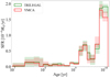 |
Fig. A.1 Comparison of the recovered SFRs of tile 3_20 using the two different models for MW foreground contamination. The red histogram shows the SFR derived using the observed YMCA tile as foreground model, while the green histogram is the SFH derived with the TRILEGAL synthetic CMD. |
To further illustrate the impact of different MW contamination modelling approaches, we present here a comparison of the SFH recovery across different tiles using both the YMCA tile and synthetic CMDs of the MW generated by TRILEGAL. We generated synthetic foreground CMDs for fields centred on the analysed tiles, each covering 1 deg2. The synthetic foreground CMD was then convolved with the incompleteness of the data and incorporated into our library of partial CMDs.
Figures A.1 and A.2 shows the recovered SFH for tiles 3_20 and 3_11, respectively, highlighting the differences introduced by the two methods. The corresponding residuals are displayed in Figures A.3 and A.4, where the TRILEGAL-based model clearly introduces systematically larger discrepancies, especially for g - i between 2 and 3 mag. The primary source of these discrepancies stems from the difficulty in accurately modelling the foreground contamination with synthetic CMDs. While TRILEGAL provides a sophisticated model for Galactic stellar populations, it lacks the ability to fully replicate the specific MW stars distribution present in our fields. In contrast, the YMCA tile directly samples the foreground contamination in a manner that is inherently consistent with the data. The residuals around the RC region in tile 3_20 are likely attributable to significant theoretical modelling uncertainties for advanced stellar evolutionary phases, particularly concerning the intricate interplay of poorly understood physical processes (e.g.: late-phase stellar winds, convection, mass loss).
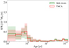 |
Fig. A.2 Same as Figure A.1 for tile 3_11. |
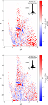 |
Fig. A.3 Comparison of the residuals’ Hess diagrams for tile 3_20 using TRILEGAL (top) and the observed YMCA tile (bottom) as foreground models. |
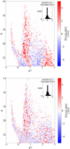 |
Fig. A.4 Same as Figure A.3 for tile 3_11. |
Appendix B CMDs of individual tiles
In Figure B.1, we present the CMDs of all the tiles included in our analysis. These deep CMDs offer an unprecedented view of the stellar populations across the Magellanic Bridge, covering the most extensive area hitherto observed. To facilitate spatial interpretation, the CMDs are arranged to reproduce the sky distribution of the tiles. A fiducial MS ridge line (red dashed) is overplotted as a reference, and an old isochrone (magenta dashed line) is added in the tiles closer to the LMC. The number of stars contributing to each CMD is reported in Table 3.
 |
Fig. B.1 CMDs of the analysed regions. We overplotted a reference isochrone representing an age of 30 Myr and [Fe/H] = −0.5 dex (red dashed line), and, from tile 3_16 onwards, an old isochrone representing an age of 8 Gyr and [Fe/H] = −1 dex (magenta dashed line). The distance modulus and extinction applied to the isochrones are those listed in Table 3 for the corresponding region. |
All Tables
Summary of the parameters used in the recovery of the SFH of each tile in the Magellanic Bridge.
All Figures
|
Fig. 1 Footprint of the STEP survey pointings (blue boxes), showing the location of the SMC body and the Bridge. The area covered by this work is highlighted in red. The LMC is in the left direction, outside the map. The black dots mark the position of star clusters and associations from the catalogue of Bica et al. (2020). |
| In the text | |
|
Fig. 2 Hess diagrams of the completeness for all analysed tiles. In each cell of the CMD the completeness is computed as the ratio of recovered ASs with respect to the number of input stars. The red line indicates the 50% completeness level. |
| In the text | |
|
Fig. 3 Difference between the output and input magnitude vs. input magnitude in g (top) and i (bottom) filters derived from AS tests for tile 3_17. The solid red line marks the median of the distributions, while the dashed lines indicate the fifth and 95th percentiles of the distributions. |
| In the text | |
|
Fig. 4 CMD of the tile 4_14 from the YMCA survey, used to model the MW contamination in our analysis. |
| In the text | |
|
Fig. 5 Stellar density distribution for Galactic longitude l = 289° across different latitude bins (−44° ≤ b ≤ −38°). Each panel displays the normalized GBP - GRP colour distribution for different magnitude intervals sourced from the TRILEGAL Galactic model (Girardi et al. 2005, 2012). The Gaia EDR3 distributions at b = −42° are plotted in gray. |
| In the text | |
|
Fig. 6 CMDs of the observed data (top left) of tile 2_11 compared with the best-fit synthetic model from PARSEC-COLIBRI (top centre) and BaSTI (top right) stellar isochrones. In the plot at the bottom we show the residuals and the comparison between the observed and recovered luminosity functions and colour distributions, as well as the distribution of residuals from the PARSEC-COLIBRI models. |
| In the text | |
|
Fig. 7 SFH of tile 2_11 recovered with PARSEC-COLIBRI (red) and BaSTI (blue) stellar isochrones. |
| In the text | |
|
Fig. 8 Map of the analysed regions overlaid with the SFH of the individual tiles. The lines connect the location of each tile on the map to its corresponding inset plot, which displays the SFR in unit of 10−4 M⊙ yr−1 resulting from the PARSEC-COLIBRI (red) and BaSTI (blue) stellar evolution libraries as a function of age in Gyr (logarithmic scale). The y-axis limits are independently scaled for each tile to better show the SFH features of each region and the axis labels were omitted for enhanced clarity. The shaded regions represent the fifth and 95th percentile uncertainties of the SFR. |
| In the text | |
|
Fig. 9 Spatial distribution of UMS stars (top), RGB and RC (centre) and HI gas column density distribution (bottom) from the GASS survey (McClure-Griffiths et al. 2009). |
| In the text | |
|
Fig. 10 Comparison between the global SFH of the Magellanic Bridge recovered using the PARSEC-COLIBRI (red line) and BaSTI (blue line) stellar models. The dashed pink line indicates a period of intense SF found by Mazzi et al. (2021); the dashed green line indicates the first synchronized SF peak of the MCs found by Massana et al. (2022) and Ruiz-Lara et al. (2020). Notice that the left portion of the abscissa is in logarithmic age scale to better appreciate the details, while the right portion is in linear scale. The shaded area represents the confidence interval of our solution, computed as the fifth and 95th percentiles of the parameters’ distribution. |
| In the text | |
|
Fig. 11 Global AMR of the Magellanic Bridge found using the PADOVA-COLIBRI (red line) and BaSTI (blue line) stellar models. The left portion of the abscissa is in logarithmic scale to better appreciate the details, while the right portion is in linear scale. The shaded area represents the confidence interval of our solution, computed as the fifth and 95th percentiles of the parameters’ distribution. The dashed green line marks the global AMR of the SMC obtained by Rubele et al. (2018), while the dashed black line represents the AMR of the LMC from Carrera et al. (2008b). |
| In the text | |
|
Fig. 12 AMR for the three observed regions, with the top, central, and bottom panels representing the LMC-side, central, and SMC-side regions, respectively. Each point corresponds to the mean metallicity within an age bin, with horizontal error bars showing the bin width. The black diamonds and orange hexagons indicate spectroscopic measurements for the SMC (Carrera et al. 2008a) and LMC (Carrera et al. 2008b), respectively. |
| In the text | |
|
Fig. 13 SF law in the Magellanic Bridge (blue triangles) in comparison with the data by Bolatto et al. (2011) (magenta filled circles) and curves of the KMT09 models (adapted from the same authors) for different values of the cZ′ parameter (the product of the gas metallicity Z′ and the degree of gas clumping c) indicated by the dash-dotted, dashed, and solid lines. |
| In the text | |
|
Fig. A.1 Comparison of the recovered SFRs of tile 3_20 using the two different models for MW foreground contamination. The red histogram shows the SFR derived using the observed YMCA tile as foreground model, while the green histogram is the SFH derived with the TRILEGAL synthetic CMD. |
| In the text | |
|
Fig. A.2 Same as Figure A.1 for tile 3_11. |
| In the text | |
|
Fig. A.3 Comparison of the residuals’ Hess diagrams for tile 3_20 using TRILEGAL (top) and the observed YMCA tile (bottom) as foreground models. |
| In the text | |
|
Fig. A.4 Same as Figure A.3 for tile 3_11. |
| In the text | |
|
Fig. B.1 CMDs of the analysed regions. We overplotted a reference isochrone representing an age of 30 Myr and [Fe/H] = −0.5 dex (red dashed line), and, from tile 3_16 onwards, an old isochrone representing an age of 8 Gyr and [Fe/H] = −1 dex (magenta dashed line). The distance modulus and extinction applied to the isochrones are those listed in Table 3 for the corresponding region. |
| In the text | |
Current usage metrics show cumulative count of Article Views (full-text article views including HTML views, PDF and ePub downloads, according to the available data) and Abstracts Views on Vision4Press platform.
Data correspond to usage on the plateform after 2015. The current usage metrics is available 48-96 hours after online publication and is updated daily on week days.
Initial download of the metrics may take a while.